1 Introduction

In the brane world scenario, our four-dimensional spacetime is realized on topological defects such as walls embedded in a higher dimensional spacetime [1]. One of the most intriguing models in the brane-world scenario is proposed by Randall and Sundrum, which offers a possibility to solve the gauge hierarchy problem by means of two walls [2], and a four-dimensional localized massless graviton on the wall [3]. The model is based on a spacetime metric containing a warp factor ${\rm e}^{2U(y)}$

$$ds^{2}=g_{\mu\nu}dx^{\mu}dx^{\nu}={\rm e}^{2U(y)}\eta_{mn}dx^{m}dx^{n}+dy^{2},$$ (1.1)

where the five-dimensional indices transforming under the general coordinate transformations are denoted by $\mu,\nu=0,1,2,3,4$, the flat four-dimensional indices $m,n=0,1,3,4$. We choose to denote the coordinate of the extra dimension $y\equiv x^{2}$. They had to introduce an orbifold, a bulk cosmological constant and a boundary cosmological constant placed at orbifold fixed points. A fine-tuning was needed between these cosmological constants.

On the other hand, supersymmetry (SUSY) has been most powerful to construct realistic models for unified theories beyond the standard model [4]. The supersymmetric version of the warped metric model with an orbifold has been worked out [5]. It is tempting to replace the orbifold by a smooth wall constructed from physical scalar fields. After many studies of BPS walls in four-dimensional ${\cal N}=1$ supergravity (SUGRA) coupled with chiral scalar multiplets [6], an exact solution of a BPS wall has been constructed [7]. Since the nonlinear models in the ${\cal N}=2$ SUGRA should have a quarternioinic Kähler target manifold [8], there must be a nontrivial gravitational deformation of the hyper-Kähler nonlinear sigma models of the global ${\cal N}=2$ SUSY theories. For massless ${\cal N}=2$ nonlinear sigma models in four dimensions, the necessary gravitational deformations have been worked out [9], [10]. However, nontrivial potential terms are needed to obtain domain wall solutions. In the ${\cal N}=2$ SUSY nonlinear sigma models, the possible potential terms are severely restricted [11]–[16]. Massive hyper-Kähler nonlinear sigma models without gravity in four dimensions have been constructed in harmonic superspace as well as in ${\cal N}=1$ superfield formulation [17], [18], and have yielded the domain wall solution for the Eguchi-Hanson manifold [19] previously obtained in the on-shell component formulation [12]. Other BPS solitons in ${\cal N}=2$ global SUSY theories such as lumps have also been constructed [20], [21].

Studies of domain walls in gauged SUGRA theories in five dimensions [22] revealed the necessity of hypermultiplets [23]. Domain walls in massive quaternionic Kähler nonlinear sigma models in the ${\cal N}=2$ SUGRA theories have been studied using mostly homogeneous target manifolds. Unfortunately, SUSY vacua in homogeneous target manifolds are not truly IR critical points, but can only be saddle points with some IR directions [24], [25]. No-go theorems are argued [26], [27], and solutions proposed [28]. Only a few nonlinear sigma models with quaternionic manifolds as target spaces admitting wall solutions have been constructed [29], [30]. However, a limit of weak gravitational coupling cannot be taken in these manifolds, contrary to the model with an exact solution in ${\cal N}=1$ SUGRA in four-dimensions [7]. This is a serious drawback for phenomenological purposes. Recently we have succeeded in constructing a smooth wall configuration which has a smooth limit of vanishing gravitational coupling [31], using the recently developed off-shell formalism of ${\cal N}=2$ SUGRA in five dimensions [32], [33]. On-shell SUGRA in five dimensions [34] as well as off-shell form without vector multiplets [35] have also been formulated previously.

The purpose of our paper is to extend our construction of exact BPS domain walls in five-dimensional SUGRA coupled with hypermultiplets (and vector multiplets), especially to higher dimensional quaternionic target spaces. We obtain a gravitational deformations of $T^{*}{\bf C}P^{n}$ nonlinear sigma models which admit multi-walls as BPS solutions. We shall call them $QT^{*}{\bf C}P^{n}$ models. These multi-wall solutions possess $2n$ parameters which is the same number as that of moduli parameters in the global SUSY case (vanishing gravitational coupling). We can take a limit of vanishing gravitational coupling smoothly as in our previous example of gravitational deformations of the $T^{*}{\bf C}P^{1}$ model (Eguchi-Hanson manifold) [31]. We also construct gravitational deformations with the $U(1)\times U(1)$ gauging of the hypermultiplets in the ${\cal N}=2$ SUGRA, which reduce to more general models than the $T^{*}{\bf C}P^{n}$ model with only $U(1)^{n}$ isometry. We shall call them generalized $QT^{*}{\bf C}P^{n}$ models. We find that they admit multi-wall BPS solutions as well. It is also observed that the isometry of the target space is enhanced at particular values of parameters. Qualitative features of the wall solutions for hypermultiplets are found to be in one-to-one correspondence with those in the global SUSY case, even though there are nontrivial gravitational corrections [13]. In addition, we obtain solutions of the warp factor. We find that possible stationary points of the warp factor are obtained as intersections with a hypersurface in field space and are easily visualized graphically. We show that the warp factor in the gravitationary dressed $T^{*}{\bf C}P^{n}$ models can have at most one stationary point.

Similarly to our previous example, we obtain three types of behavior of the warp factor : 1) decreasing for both infinities of extra dimension $y\rightarrow\pm\infty$, interpolating two infrared (IR) fixed points, 2) decreasing in one direction, and flat in the other, interpolating an IR fixed point and flat space, 3) decreasing in one direction, and increasing in the other, interpolating an IR and an ultra-violet (UV) fixed points. The IR-IR case may be desirable for phenomenological purposes [36], but other cases are also interesting in view of the AdS/CFT correspondence [37].

We can take a thin-wall limit of our solitons (domain walls) in five-dimensional SUGRA which gives orbifold type models similar to the Randall-Sundrum model. We find that the relation between bulk and boundary cosmological constants is now realized as an automatic consequence of the solution of dynamical equations rather than a fine-tuning between input parameters [31], similarly to the BPS wall solution in the four-dimensional SUGRA [7]. The four-dimensional graviton should be localized also on our wall solution [38].

In constructing a gravitational deformation of nonlinear sigma models, we followed the strategy of our previous paper by using the off-shell formulation of five-dimensional SUGRA (tensor calculus) [32], [33]. We combine this formalism with the quotient method via a vector multiplet without kinetic term and the massive deformation (central charge extension). In the off-shell formulation, we can easily introduce the gravitational coupling to the massive hypermultiplets with linear kinetic term which is interacting with the vector multiplet without kinetic term. By eliminating the vector multiplet after coupling to gravity, we automatically obtain a gravitationally deformed constraint resulting in inhomogeneous quaternionic Kähler nonlinear sigma model with the necessary potential terms. We may call the procedure a massive quaternionic Kähler quotient method. As an extension to our previous model [31], we introduce many more hypermultiplets, but retain the same number of vector multiplets to gauge the hypermultiplet target space. Therefore we obtain higher dimensional quaternionic Kähler manifolds as target space. Although we have obtained legitimate quaternionic manifolds by construction at least locally, we have not yet explored possible global singularities which was noticed in the case of the $T^{*}{\bf C}P^{1}$ model (Eguchi-Hanson manifold) [10], [31]. As we have argued before [31], we can restore the kinetic term of the vector multiplet to avoid such singularities if they exist. Our BPS solutions should still be valid solutions even with the kinetic term for the vector multiplet.

Sec.2 summarizes the massive quaternionic Kähler quotient method in the off-shell formulation of SUGRA, and introduces the general $U(1)\times U(1)$ gauging leading to $4n$ (real) dimensional quaternionic nonlinear sigma models. Sec.3 gives vacua and BPS equations of the model. Sec.4 discusses general properties of BPS solutions and presents exact multi-wall solutions. Sec.5 discusses the weak gravity limit and other issues.

2 Our model

2.1 Five-dimensional Supergravity

Our model is based on the off-shell formulation of Poincaré SUGRA in five-dimensions with hypermultiplets and vector multiplets. The Poincaré SUGRA is most conveniently obtained from a gauge fixing of superconformal gravity [32], which comes from gauging the translation $P_{a}$, supersymmetry $Q_{i}$, local Lorentz transformation $M_{ab}$, dilatation $D$, $SU(2)_{R}$ transformation $U_{ij}$, conformal supersymmetry $S_{i}$ and special conformal boost $K_{a}$ where $a=0,\dots,4$ denote local Lorentz indices in five dimensions, and $i,j=1,2$ denote $SU(2)_{R}$ indices. Some of these gauge fields are written in terms of other fields (become auxiliary fields) after imposing appropriate constraints, and the resulting superconformal gravity contains the Weyl multiplet consisting of vielbein $e_{\mu}{}^{a}$, gravitino $\psi_{\mu}^{i}$, $SU(2)_{R}$ gauge field $V_{\mu}^{ij}$, and the additional fields to balance the bosonic and fermionic degrees of freedom, namely a real antisymmetric tensor field $v_{ab}$, an $SU(2)$-Majorana spinor field $\chi^{i}$, and a real scalar field $D$. Altogether the Weyl multiplet consists of the $32$ bosonic and $32$ fermionic components [32], [33].

In global ${\cal N}=2$ SUSY case, BPS wall solutions have been obtained by using $n+1$   ($n\geq 1$) hypermultiplets as matter fields [12], [13], [17], [18]. To obtain nontrivial interactions among hypermultiplets, the nonlinearity of the kinetic term (SUSY nonlinear sigma model) is required [39]. The most practical way to obtain the nonlinear sigma model is to introduce a vector multiplet without a kinetic term that provides constraints to hypermultiplets. After solving the constraints, one obtains the curved target space for hypermultiplets that becomes a hyper-Kähler manifold with real $4n$ dimension [40], [41], [17], [18]. To obtain wall solutions, we need also a nontrivial potential term among hypermultiplets. This comes about if we consider the central charge extension in the SUSY algebra producing the mass term [42]. The above method to obtain the nonlinear sigma model with a potential term is called the massive hyper-Kähler quotient method [17], [18].

To embed such a massive SUSY nonlinear sigma model into SUGRA, we need to introduce an additional hypermultiplet (with a negative metric) that is called the compensator, since the gauge fixing in conformal supergravity (dilatation, $SU(2)_{R}$ and so forth) eliminates degrees of freedom of one hypermultiplet. The nontrivial potential term is obtained by introducing the mass term through the central charge extension. This central charge extension in SUGRA should be performed through an introduction of central charge vector multiplet [32], [33] with the $U(1)$ gauge boson $W_{\mu}^{0}$, the generator $t_{0}$ and the gauge coupling $g_{0}$. After the gauge fixing from conformal supergravity, the resulting target space of physical hypermultiplets in Poincaré SUGRA becomes a projective quaternionic manifold in contrast to the flat target space in the case of global SUSY theories [32]. To obtain a curved target space of nonlinear sigma models in the globally SUSY case, we have introduced a vector multiplet without kinetic term to serve as a Lagrange multiplier field [17], [18]. Similarly, the constraint on hypermultiplets is introduced in SUGRA theories by a vector multiplet without kinetic term, whose gauge boson, generator and coupling are denoted by $W_{\mu}^{1}$, $t_{1}$ and $g_{1}$. In this paper we introduce $U(1)$ gauge field as $W_{\mu}^{1}$. Consequently, we need to introduce $U(1)\times U(1)$ vector multiplets besides the Weyl multiplets and $n+2$ hypermultiplets.

The $n+2$ hypermultiplets can be assembled into a $2$ by $2(n+2)$ matrix whose scalar components are denoted as ${\cal A}_{i}{{}^{\alpha}},\;i=1,2$. The hypermultiplet target space indices are denoted as $\alpha=1,\dots,2(n+2)$. We have $4(n+2)$ real degrees of freedom in scalar fields ${\cal A}_{i}{}^{\alpha}$, because of the reality condition [32]

$${\cal A}^{i}{}_{\alpha}\equiv\epsilon^{ij}{\cal A}_{j}{}^{\beta}\rho_{\beta\alpha}=-({\cal A}_{i}{}^{\alpha})^{*},\qquad\rho_{\alpha\beta}=\rho^{\alpha\beta}=\left(\begin{array}[]{ccc}i\sigma_{2}&&\\ &&{\bf{1}}_{n+1}\\ &-{\bf{1}}_{n+1}&\end{array}\right),$$ (2.1)

where $\epsilon^{ij}=i\sigma_{2}$ and ${\bf{1}}_{n+1}$ is the $(n+1)\times(n+1)$ unit matrix.

After integrating out a part of the auxiliary fields by their on-shell conditions in the off-shell SUGRA action [33], we obtain the bosonic part of the action for our model

$$e^{-1}{\cal L} \!\!\!= \!\!\!-\frac{1}{2\kappa^{2}}R-\frac{1}{4}F_{\mu\nu}^{0}F^{0\mu\nu}+{c\over 8}\epsilon^{\lambda\mu\nu\rho\sigma}W_{\lambda}^{0}F_{\mu\nu}^{0}F_{\rho\sigma}^{0}$$ (2.2)

$$\!\!\!-\nabla^{a}{\cal A}_{i}{{}^{\bar{\alpha}}}\nabla_{a}{\cal A}^{i}{{}_{\alpha}}-\kappa^{2}[{\cal A}_{i}{{}^{\bar{\alpha}}}\nabla_{a}{\cal A}^{j}{{}_{\alpha}}][{\cal A}^{i{\bar{\beta}}}\nabla^{a}{\cal A}_{j\beta}]$$

$$\!\!\!+{\cal A}_{i}{{}^{\bar{\alpha}}}\left[(g_{I}M^{I}t_{I})^{2}\right]_{\alpha}{}^{\beta}{\cal A}^{i}{}_{\beta}+\frac{\kappa^{2}}{12}(M^{I}{\cal Y}_{I}{{}^{ij}})(M^{I}{\cal Y}_{I{ij}}),$$

where

$$\begin{array}[]{l}{\cal A}_{i}{{}^{\bar{\alpha}}}\equiv{\cal A}_{i}{{}^{\beta}}d_{\beta}{{}^{\alpha}},\\ \nabla_{\mu}{\cal A}_{i}{{}^{\alpha}}=\partial_{\mu}{\cal A}_{i}{{}^{\alpha}}-(g_{I}W^{I}_{\mu}t_{I})^{\alpha}{}_{\beta}{\cal A}_{i}{}^{\beta},\\ F_{\mu\nu}^{0}=\partial_{\mu}W_{\nu}^{0}-\partial_{\nu}W_{\mu}^{0},\\ {\cal Y}_{I}{{}^{ij}}=2g_{I}{\cal A}^{(i}{{}_{\alpha}}d^{\alpha}{{}_{\beta}}(t_{I})^{\beta\gamma}{\cal A}^{j)}{{}_{\gamma}}.\end{array}$$ (2.7)

Here, we follow the notation that $d_{\alpha}{}^{\beta}=diag(\mbox{\boldmath$1$}_{2},-\mbox{\boldmath$1$}_{n+1},-\mbox{\boldmath$1$}_{n+1})$, $\kappa$ is the five-dimensional gravitational coupling, $c$ is the coefficient of the trilinear ‘norm function’ which appears in the Chern-Simons term and $I$ runs $0,1$. The $M_{I}$ denote scalar fields in vector multiplets and the auxiliary fields ${\cal Y}_{I}{{}^{ij}}$ in vector multiplets are determined by their equations of motion. We drop the kinetic term of $W^{1}_{\mu}$ here. Moreover, this gives a constraint on hypermultiplet target space through the on-shell condition of the auxiliary field ${\cal Y}_{1}{{}^{ij}}$:

$${1\over g_{1}}{\cal Y}_{1}{{}^{ij}} = 2{\cal A}^{(i}{{}_{\alpha}}d^{\alpha}{}_{\gamma}(t_{1})^{\gamma\beta}{\cal A}^{j)}{{}_{\beta}}\rightarrow 0\qquad\left(g_{1}\rightarrow\infty\right).$$ (2.8)

This constraint (2.8) corresponds to the constraint for Eguchi-Hanson target space in the limit of $\kappa\to 0$ in the $n=1$ case Ref.[17], [18]. The gauge fixing of dilatation in superconformal gravity gives an additional constraint on hypermultiplet scalars as (with ${\cal A}_{i}{{}^{\bar{\alpha}}}\equiv{\cal A}_{i}{{}^{\beta}}d_{\beta}{{}^{\alpha}}$ in Eq.(2.3))

$${\cal A}^{2} \equiv {\cal A}_{i}{{}^{\bar{\alpha}}}{\cal A}^{i}{{}_{\alpha}}=-2\kappa^{-2}.$$ (2.9)

Because of the quadratic form constraint (2.9), the target space manifold becomes $USp(2,2(n+1))/(U(2)\times U(2(n+1)))$ that has an isometry $USp(2,2(n+1))$ which is defined by the invariance of the quadratic form (2.9) [32],

$$t^{\dagger}d+dt=0,\qquad t^{\rm T}\rho-\rho t^{\dagger}=0,$$ (2.10)

where $t$ denotes the generator of the isometry group. The general form of $t$ satisfying these constraints is given by :

$$t^{\alpha}{{}_{\beta}}=\left(\begin{array}[]{ccc}\mbox{\boldmath$A$}&\mbox{\boldmath$B$}^{\dagger}&-\varepsilon\mbox{\boldmath$B$}^{\rm T}\\ \mbox{\boldmath$B$}&\tilde{\mbox{\boldmath$D$}}&\mbox{\boldmath$C$}\\ \mbox{\boldmath$B$}^{*}\varepsilon&\mbox{\boldmath$C$}^{*}&-\tilde{\mbox{\boldmath$D$}}^{\rm T}\end{array}\right),$$ (2.14)

where $A$ is a $2$ by $2$ matrix satisfying, $\mbox{\boldmath$A$}^{\dagger}=-\mbox{\boldmath$A$}$ and $\mbox{\boldmath$A$}=\varepsilon\mbox{\boldmath$A$}^{\rm T}\varepsilon$, $B$ is a $(n+1)$ by $2$ matrix, $C$ is a $(n+1)$ by $(n+1)$ matrix satisfying $\mbox{\boldmath$C$}^{\rm T}=-\mbox{\boldmath$C$}$, and $\tilde{\mbox{\boldmath$D$}}$ is a $(n+1)$ by $(n+1)$ matrix satisfying $\tilde{\mbox{\boldmath$D$}}^{\dagger}=-\tilde{\mbox{\boldmath$D$}}$.

We should choose gauge generators $t_{I}$ for vector multiplets $W_{\mu}^{I}$ as one of the generators $t$ of the isometry $USp(2,2(n+1))$. Since we are interested in $U(1)\times U(1)$ gauging, we choose two commuting diagonal generators parametrized by

$$\left(t_{I}\right)^{\alpha}{{}_{\beta}}=\left(\begin{array}[]{ccc}i\alpha_{I}\sigma_{3}&&\\ &i\mbox{\boldmath$D$}_{I}&\\ &&-i\mbox{\boldmath$D$}_{I}\end{array}\right),\quad\quad\left(I=0,1\right)$$ (2.18)

where $\sigma_{3}$ is one of the Pauli matrices, $\mbox{\boldmath$D$}_{I}=diag(d_{I,1},d_{I,2},\cdots,d_{I,n+1})$, with $d_{I,a}$ and $\alpha_{I}$ are real parameters. We again stress that gauging by $t_{1}$ gives the non-minimal kinetic term for hypermultiplet scalar fields ${\cal A}_{i}{}^{\alpha}$ through the constraint. Therefore the target manifold of the hypermultiplet nonlinear sigma model is entirely determined by the choice of $t_{1}$. On the other hand, the gauging by $t_{0}$ produces a nontrivial potential for hypermultiplet scalar fields ${\cal A}_{i}{}^{\alpha}$.

Let us clarify the meaning of parameters $\alpha_{I}$ and $d_{I,\alpha}$. We wish to demand that our model should have a well-defined limit of vanishing gravitational coupling. The compensator hypermultiplet ${\cal A}_{i}{}^{\alpha}$ with $\alpha=1,2$ has negative norm and should disappear in the vanishing gravitational coupling. This requires $\alpha_{I}$ in $t_{I}$ should vanish in the limit $\kappa\rightarrow 0$. On the other hand, we wish to recover a nonlinear sigma model with the constraint given by the part of $(t_{1})^{\alpha}{}_{\beta}$ with $\alpha,\beta=3,\cdots,2(n+2)$. Similarly the potential for the hypermultiplets except the compensator is given by the part of $t_{0}$ with $\alpha,\beta=3,\cdots,2(n+2)$. Therefore $d_{I,a}$ should have a finite limit as $\kappa\rightarrow 0$. Even accepting these requirements, we still have a considerable freedom to choose parameters. For instance, a general choice for $\alpha_{1}$ and $d_{1,a}$ makes the target manifold with only $U(1)^{n}$ isometry and in general inhomogeneous through the constraint (2.8). We shall call this case as the asymmetric kinetic term. We will consider BPS multi-wall solutions in such generic models. If we take a symmetric choice of parameters

$$d_{1,a}=d_{1,n+1},\qquad a=1,2,\cdots,n,$$ (2.19)

the kinetic term becomes symmetric and the target manifold admits much larger isometry, $SU(n+1)$ in this case. This is the case of the usual $T^{*}{\bf C}P^{n}$ nonlinear sigma model in the limit of vanishing gravitational coupling. We shall call this case as the symmetric kinetic term. On the other hand, we can obtain other target manifolds with enhanced isometry, if we abandon the weak gravity limit. We find that too much enhanced isometry often results in pathological behaviors such as runaway vacuum. A systematic search of possibilities for $n=1$ case is given in Appendix A.

By reversing the sign of the third line of (2.2), we obtain a scalar potential consisting of two terms : the first term arises from the couplings of hypermultiplets to scalars $M^{0},M^{1}$ in vector multiplets and the second term from eliminating the auxiliary fields of the $U(1)$ vector multiplet with kinetic term ($W_{\mu}^{0}$). The requirement of minimal kinetic term for the gauge field $W_{\mu}^{0}$ together with the canonical normalization of the Einstein-Hilbert term in Eq.(2.2) determine the value of the associated scalar $M^{0}$ as

$$(M^{0})^{2}=\frac{3}{2}\kappa^{-2}.$$ (2.20)

As we will see in later sections, the parameter $g_{0}M^{0}$ gives the scale of width of the wall and should be kept finite when taking the weak gravity limit $\kappa\rightarrow 0$. Therefore the gauge coupling $g_{0}$ of the central charge vector multiplet must be proportional to $\kappa$ for vanishing gravitational coupling. This fact implies that the central charge vector multiplet decouples in the global SUSY model. This result is in accord with the fact that the global SUSY model does not need the central charge vector multiplet to generate mass terms.

The scalar $M^{1}$ and the gauge field $W^{1}_{\mu}$ without kinetic term is a Lagrange multiplier, which is determined by its algebraic equations of motion as

$$g_{1}M^{1} = -\frac{{\cal A}_{i}{{}^{\bar{\alpha}}}(t_{0}t_{1})_{\alpha}{}^{\beta}{\cal A}^{i}{}_{\beta}}{{\cal A}_{i}{{}^{\bar{\alpha}}}[(t_{1})^{2}]_{\alpha}{}^{\beta}{\cal A}^{i}{}_{\beta}}g_{0}M^{0}\equiv f({\cal A})g_{0}M^{0},$$ (2.21)

$$g_{1}W^{1}_{\mu} = \frac{1}{2}\frac{{\cal A}_{i}{{}^{\bar{\alpha}}}\overset{\leftrightarrow}{\partial}_{\mu}t_{1\alpha}{}^{\beta}{\cal A}^{i}{}_{\beta}}{{\cal A}_{i}{{}^{\bar{\alpha}}}[(t_{1})^{2}]_{\alpha}{}^{\beta}{\cal A}^{i}{}_{\beta}}.$$ (2.22)

2.2 Bosonic action for Hypermultiplets

Assuming $W_{\mu}^{0}=0$, we rewrite the on-shell bosonic action of the hypermultiplets:

$$e^{-1}{\cal L}_{matter} = -\partial^{\mu}{\cal A}_{i}{{}^{\bar{\alpha}}}\partial_{\mu}{\cal A}^{i}{{}_{\alpha}}-\kappa^{2}\left({\cal A}^{i\bar{\alpha}}\overset{\leftrightarrow}{\partial}_{\mu}{\cal A}^{j}{{}_{\alpha}}\right)^{2}+(g_{1}W_{\mu}^{1})^{2}{\cal A}_{i}{{}^{\bar{\alpha}}}\left(t_{1}{{}^{2}}\right)_{\alpha}{}^{\beta}{\cal A}^{i}_{\beta}-V({\cal A}_{i}{{}^{\alpha}}),$$ (2.23)

$$V({\cal A}_{i}{{}^{\alpha}}) = -{\cal A}_{i}{{}^{\bar{\alpha}}}\left[\left(g_{I}M^{I}t_{I}\right)^{2}\right]_{\alpha}{}^{\beta}{\cal A}^{i}{}_{\beta}-\frac{\kappa^{2}}{12}(M^{0})^{2}\mathcal{Y}_{0}{{}^{ij}}\mathcal{Y}_{0{ij}},$$ (2.24)

where $M^{1}$ and $W^{1}_{\mu}$ are given in Eq.(2.21) and (2.22). By using the $SU(2)_{R}$ gauge fixing, we can choose the first two columns in the hypermultiplet matrix ${\cal A}_{i}{{}^{\alpha}}$ to be proportional to the two by two unit matrix. Remaining components of ${\cal A}_{i}{}^{\alpha}$ can be parametrized by two $(n+1)$-component complex fields $\phi_{i}{{}^{a}}$ with $i=1,2$ and $a=1,2,\cdots,n+1$

$${\cal A}_{i}{}^{\alpha}\equiv\frac{1}{\kappa}\bar{\cal A}^{-1/2}\left(\begin{array}[]{cccc}1&0&\kappa\mbox{\boldmath$\phi$}_{1}^{T}&-\kappa\mbox{\boldmath$\phi$}_{2}^{*T}\\ 0&1&\kappa\mbox{\boldmath$\phi$}_{2}^{T}&\kappa\mbox{\boldmath$\phi$}_{1}^{*T}\\ \end{array}\right),\quad\mbox{\boldmath$\phi$}_{i}=\left(\begin{array}[]{c}\phi_{i}{{}^{1}}\\ \phi_{i}{{}^{2}}\\ \vdots\\ \phi_{i}{{}^{n+1}}\end{array}\right)=(\phi_{i}{{}^{a}}).$$ (2.31)

$$\bar{\cal A}=1-\kappa^{2}(|\mbox{\boldmath$\phi$}_{1}|^{2}+|\mbox{\boldmath$\phi$}_{2}|^{2})$$ (2.32)

which satisfies the constraint (2.9). This parametrization is a generalization of that used by Curtright and Freedman for $T^{*}{\bf C}P^{1}$ nonlinear sigma model ($n=1$ case) [44]. We shall call it the (generalized) Curtright-Freedman basis.

In terms of the Curtright-Freedman basis with the generators (2.18), $\mathcal{Y}_{I}{{}^{ij}}$ can be expressed as

$$\mathcal{Y}_{I}{{}^{ij}}=-2g_{I}\bar{\cal A}^{-1}\left(\begin{array}[]{cc}2i{\cal S}_{I}&i{\cal T}_{I}\\ i{\cal T}_{I}&-2i{\cal S}_{I}^{*}\end{array}\right).$$ (2.35)

where we define

$${\cal T}_{I} \equiv \kappa^{-2}\alpha_{I}-\left(\mbox{\boldmath$\phi$}_{1}^{\dagger}\mbox{\boldmath$D$}_{I}\mbox{\boldmath$\phi$}_{1}-\mbox{\boldmath$\phi$}_{2}^{\dagger}\mbox{\boldmath$D$}_{I}\mbox{\boldmath$\phi$}_{2}\right),$$ (2.36)

$${\cal S}_{I} \equiv \mbox{\boldmath$\phi$}_{1}^{\dagger}\mbox{\boldmath$D$}_{I}\mbox{\boldmath$\phi$}_{2}.$$ (2.37)

Hence, the constraint (2.8) reduces to

$${\cal T}_{1}=0,\qquad{\cal S}_{1}={\cal S}_{1}^{*}=0.$$ (2.38)

Finally, we obtain the bosonic Lagrangian in terms of the Curtright-Freedman basis as follows:

$$\frac{1}{2}e^{-1}{\cal L}_{matter} \!\!\!= \!\!\!-\bar{\cal A}^{-1}[|\partial_{\mu}\mbox{\boldmath$\phi$}_{1}|^{2}+|\partial_{\mu}\mbox{\boldmath$\phi$}_{2}|^{2}+(\kappa^{-2}\alpha_{1}^{2}-\mbox{\boldmath$\phi$}_{1}^{\dagger}\mbox{\boldmath$D$}_{1}^{2}\mbox{\boldmath$\phi$}_{1}-\mbox{\boldmath$\phi$}_{2}^{\dagger}\mbox{\boldmath$D$}_{1}^{2}\mbox{\boldmath$\phi$}_{2})W^{1}_{\mu}W^{1\mu}]$$ (2.39)

$$\!\!\!\!-\kappa^{2}\bar{\cal A}^{-2}[|\mbox{\boldmath$\phi$}_{2}^{\dagger}\partial_{\mu}\mbox{\boldmath$\phi$}_{2}+\mbox{\boldmath$\phi$}_{1}^{\rm T}\partial_{\mu}\mbox{\boldmath$\phi$}_{1}^{*}|^{2}+|\mbox{\boldmath$\phi$}_{1}^{\rm T}\partial_{\mu}\mbox{\boldmath$\phi$}_{2}^{*}-\mbox{\boldmath$\phi$}_{2}^{\dagger}\partial_{\mu}\mbox{\boldmath$\phi$}_{1}|^{2}]-\frac{1}{2}V(\phi_{i}{{}^{a}}),$$

$$\frac{1}{2}V(\phi_{i}{{}^{a}}) \!\!\!= \!\!\!\!(g_{0}M^{0})^{2}\bar{\cal A}^{-1}\left[-\kappa^{-2}\alpha^{2}\!+\!\left(\mbox{\boldmath$\phi$}_{1}^{\dagger}\mbox{\boldmath$D$}^{2}\mbox{\boldmath$\phi$}_{1}+\mbox{\boldmath$\phi$}_{2}^{\dagger}\mbox{\boldmath$D$}^{2}\mbox{\boldmath$\phi$}_{2}\right)\!-\!\frac{\kappa^{2}}{3}\bar{\cal A}^{-1}\left({\cal T}_{0}^{2}+4|{\cal S}_{0}|^{2}\right)\!\right],$$ (2.40)

where we define quantities combining two vector multiplets using $f$ in Eq.(2.21)

$$\alpha\equiv\alpha_{0}+f\alpha_{1},\qquad d_{a}\equiv d_{0,a}+fd_{1,a},\qquad\mbox{\boldmath$D$}\equiv\mbox{\boldmath$D$}_{0}+f\mbox{\boldmath$D$}_{1}=diag\{d_{a}\}.$$ (2.41)

We obtain the following useful expression:

$$g_{I}M^{I}t_{I}=g_{0}M^{0}(t_{0}+ft_{1})=g_{0}M^{0}\left(\begin{array}[]{ccc}i\alpha\sigma_{3}&&\\ &i\mbox{\boldmath$D$}&\\ &&-i\mbox{\boldmath$D$}\end{array}\right).$$ (2.45)

We can express $W^{1}_{\mu}$ and $f$ as follows:

$$g_{1}W^{1}_{\mu} = \frac{i}{2}\frac{\mbox{\boldmath$\phi$}_{1}^{\dagger}\mbox{\boldmath$D$}_{1}\overset{\leftrightarrow}{\partial}_{\mu}\mbox{\boldmath$\phi$}_{1}+\mbox{\boldmath$\phi$}_{2}^{\dagger}\mbox{\boldmath$D$}_{1}\overset{\leftrightarrow}{\partial}_{\mu}\mbox{\boldmath$\phi$}_{2}}{\kappa^{-2}\alpha_{1}^{2}-\left(\mbox{\boldmath$\phi$}_{1}^{\dagger}\mbox{\boldmath$D$}_{1}^{2}\mbox{\boldmath$\phi$}_{1}+\mbox{\boldmath$\phi$}^{\dagger}_{2}\mbox{\boldmath$D$}_{1}^{2}\mbox{\boldmath$\phi$}_{2}\right)},$$ (2.46)

$$f = -\frac{\kappa^{-2}\alpha_{0}\alpha_{1}-\left(\mbox{\boldmath$\phi$}_{1}^{\dagger}\mbox{\boldmath$D$}_{0}\mbox{\boldmath$D$}_{1}\mbox{\boldmath$\phi$}_{1}+\mbox{\boldmath$\phi$}_{2}^{\dagger}\mbox{\boldmath$D$}_{0}\mbox{\boldmath$D$}_{1}\mbox{\boldmath$\phi$}_{2}\right)}{\kappa^{-2}\alpha_{1}^{2}-\left(\mbox{\boldmath$\phi$}_{1}^{\dagger}\mbox{\boldmath$D$}_{1}^{2}\mbox{\boldmath$\phi$}_{1}+\mbox{\boldmath$\phi$}_{2}^{\dagger}\mbox{\boldmath$D$}_{1}^{2}\mbox{\boldmath$\phi$}_{2}\right)},$$ (2.47)

where $\mbox{\boldmath$\phi$}_{1}^{\dagger}\overset{\leftrightarrow}{\partial}_{\mu}\mbox{\boldmath$\phi$}_{1}\equiv\mbox{\boldmath$\phi$}_{1}^{\dagger}{\partial}_{\mu}\mbox{\boldmath$\phi$}_{1}-({\partial}_{\mu}\mbox{\boldmath$\phi$}_{1}^{\dagger})\mbox{\boldmath$\phi$}_{1}$.

3 BPS equations

3.1 SUSY Vacuum

For a stable BPS solution two or more isolated SUSY vacua are needed. We investigate the vacuum structure of our model in this subsection. The on-shell supertransformation for the fermionic fields are of the form:

$$\delta_{\varepsilon}\psi^{i}_{\mu} = {\cal D}_{\mu}\varepsilon^{i}-\frac{\kappa^{2}}{6}\gamma_{\mu}M^{I}{\cal Y}_{I}{{}^{i}}{{}_{j}}\varepsilon^{j},$$ (3.1)

$$\delta_{\varepsilon}\zeta^{\alpha} = -\gamma^{\mu}{\cal D}_{\mu}{\cal A}_{i}{{}^{\alpha}}\varepsilon^{i}-g_{I}M^{I}(t_{I}{\cal A}_{i})^{\alpha}\varepsilon^{i}+\frac{\kappa^{2}}{2}{\cal A}_{j}{{}^{\alpha}}M^{I}{\cal Y}_{I}{{}^{j}}{{}_{i}}\varepsilon^{i},$$ (3.2)

where ${\cal D}_{\mu}\varepsilon^{i}=\left(\partial_{\mu}-\frac{1}{4}\gamma_{ab}\omega_{\mu}{{}^{ab}}\right)\varepsilon^{i}-\kappa^{2}V_{\mu}{{}^{i}}{{}_{j}}\varepsilon^{j}$, ${\cal D}_{\mu}{\cal A}_{i}{{}^{\alpha}}=\nabla_{\mu}{\cal A}_{i}{{}^{\alpha}}-\kappa^{2}V_{\mu i}{{}^{j}}{\cal A}_{j}{{}^{\alpha}}$ and $V_{\mu}{{}^{ij}}=-\frac{1}{2}{\cal A}^{i\bar{\alpha}}\overset{\leftrightarrow}{\partial}_{\mu}{\cal A}^{j}{{}_{\alpha}}$. SUSY vacua conditions are obtained by demanding ‘supersymmetric’ spacetime independent background configuration for scalar fields ${\cal A}_{i}{{}^{\alpha}}$ in Eq.(3.2). This yields the following condition:

$$0=\delta_{\varepsilon}\zeta^{\alpha}\quad\Rightarrow\quad(g_{I}M^{I}t_{I}{\cal A}_{i})^{\alpha}=\frac{\kappa^{2}}{2}{\cal A}_{j}{{}^{\alpha}}M^{0}{\cal Y}_{0}{{}^{j}}{{}_{i}},$$ (3.3)

in the right hand side we used the constraint ${\cal Y}_{1}=0$ in Eq.(2.8). In terms of the Curtright-Freedman basis this can be rewritten as

$$g_{0}\left(\begin{array}[]{cc}i\alpha&0\\ 0&-i\alpha\\ i\kappa\mbox{\boldmath$D$}\mbox{\boldmath$\phi$}_{1}&i\kappa\mbox{\boldmath$D$}\mbox{\boldmath$\phi$}_{2}\\ i\kappa\mbox{\boldmath$D$}\mbox{\boldmath$\phi$}_{2}^{*}&-i\kappa\mbox{\boldmath$D$}\mbox{\boldmath$\phi$}_{1}^{*}\end{array}\right)=-\frac{\kappa^{2}}{2}\left(\begin{array}[]{cc}\mathcal{Y}_{0}{{}^{12}}&-\mathcal{Y}_{0}{{}^{11}}\\ \mathcal{Y}_{0}{{}^{22}}&-\mathcal{Y}_{0}{{}^{21}}\\ \kappa\left(\mathcal{Y}_{0}{{}^{12}}\mbox{\boldmath$\phi$}_{1}+\mathcal{Y}_{0}{{}^{22}}\mbox{\boldmath$\phi$}_{2}\right)&-\kappa\left(\mathcal{Y}_{0}{{}^{11}}\mbox{\boldmath$\phi$}_{1}+\mathcal{Y}_{0}{{}^{21}}\mbox{\boldmath$\phi$}_{2}\right)\\ \kappa\left(\mathcal{Y}_{0}{{}^{22}}\mbox{\boldmath$\phi$}_{1}^{*}-\mathcal{Y}_{0}{{}^{12}}\mbox{\boldmath$\phi$}_{2}^{*}\right)&-\kappa\left(\mathcal{Y}_{0}{{}^{21}}\mbox{\boldmath$\phi$}_{1}^{*}-\mathcal{Y}_{0}{{}^{11}}\mbox{\boldmath$\phi$}_{2}^{*}\right)\end{array}\right).$$ (3.12)

From the compensator components in the first and second rows, we find two conditions on the quantities defined in Eq.(2.35)

$${\cal T}_{0}=\kappa^{-2}\alpha\bar{\cal A},\quad{\cal S}_{0}=0.$$ (3.13)

Using these conditions, we find a condition for $\phi_{i}{{}^{a}}$ as an eigenvalue equation for the matrix $D$ :

$$\mbox{\boldmath$D$}\left(\begin{array}[]{c}\mbox{\boldmath$\phi$}_{1}\\ \mbox{\boldmath$\phi$}_{2}\end{array}\right)=\alpha\left(\begin{array}[]{c}\mbox{\boldmath$\phi$}_{1}\\ -\mbox{\boldmath$\phi$}_{2}\end{array}\right).$$ (3.18)

For a generic choice of the parameters the diagonal matrix $D$ should have no identical entries : $d_{a}\neq d_{b}$. Then the last condition yields $2(n+1)$ candidates for discrete SUSY vacua such that the only one component of $\mbox{\boldmath$\phi$}_{i}$ is non zero and all the others components vanish. The vacuum expectation value (VEV) of the nonvanishing component $\phi_{i}{{}^{a}}$ in the $a$-th vacuum is determined through the equation $d_{a}=\pm\alpha$ ($+$ is for $\mbox{\boldmath$\phi$}_{i=1}$ and $-$ is for $\mbox{\boldmath$\phi$}_{i=2}$). More explicitly, this reduces to

$$\left(\alpha_{0}d_{1,a}-d_{0,a}\alpha_{1}\right)\left(d_{1,a}|\phi_{i}{{}^{a}}|^{2}\mp\kappa^{-2}\alpha_{1}\right)=0.$$ (3.19)

Therefore, the VEV at the $a$-th vacuum is given by

$$m_{a}\equiv\frac{\kappa^{-2}\alpha_{1}}{d_{1,a}}$$ (3.20)

Since $|\phi_{i}{{}^{a}}|^{2}\geq 0$, the $a$-th vacuum with $a=1,2,\cdots,n+1$ is realized either by

$$|\phi_{1}{{}^{b}}|^{2} = m_{a}\delta^{b}{{}_{a}},\ {\rm and}\ \mbox{\boldmath$\phi$}_{2}=0,$$ (3.21)

in the case of $d_{1,a}\alpha_{1}>0$, or by

$$|\phi_{2}{{}^{b}}|^{2} = -m_{a}\delta^{a}{{}_{b}},\ {\rm and}\ \mbox{\boldmath$\phi$}_{1}=0,$$ (3.22)

in the case of $d_{1,a}\alpha_{1}<0$. In what follows, we will choose without loss of generality $d_{1,a}\alpha_{1}>0$, which implies the $n+1$ isolated SUSY vacua given in Eq.(3.21). Note that these SUSY vacua satisfy the constraint ${\cal T}_{1}={\cal S}_{1}=0$ in Eq.(2.38) and remaining vacuum condition ${\cal T}_{0}=\kappa^{-2}\alpha\bar{\cal A}$ and ${\cal S}_{0}=0$ in Eq.(3.13). In order for these VEV’s $m_{a}$ defined in Eq.(3.20) to be finite in the weak gravity limit, we must require $\alpha_{1}$ to be proportional to $\kappa^{2}$ in the limit of vanishing gravitational coupling $\kappa\rightarrow 0$.

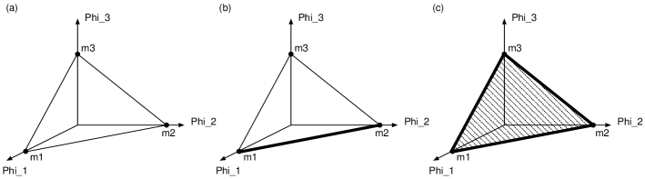
Figure 1: The SUSY vacuum structure for $n=2$ is shown. Three isolated vacua 1,2,and 3 are shown in (a). An isolated vacuum 3 and a (1, 2) degenerate vacuum are shown in (b). A (1, 2, 3) degenerate vacuum is shown in (c).

It is useful to introduce a geometrical picture of field space in order to clarify the structure of these SUSY vacuum. We make the ansatz

$$\mbox{\boldmath$\phi$}_{2}=0,$$ (3.23)

assuming $d_{1,a}\alpha_{1}>0$. Then the one of the constraint ${\cal S}_{1}=0$ is automatically satisfied. Another constraint ${\cal T}_{1}=0$ is most conveniently expressed by using modulus squared variables

$$\Phi^{a}\equiv|\phi_{1}{{}^{a}}|^{2},$$ (3.24)

$$1=\sum_{b=1}^{n+1}\frac{\Phi^{b}}{m_{b}}.$$ (3.25)

This means that the field space is restricted to the non-negative portion of an $n$ dimensional hyperplane in the $n+1$ dimensional space. We call this hyperplane $\Sigma_{1}^{(n)}$. Namely, $\Sigma_{1}^{(n)}$ is an $n$ simplex :

$$\Sigma_{1}^{(n)}=\left\{\mbox{\boldmath$\Phi$}\in\mathbb{R}^{n}\ \bigg{|}\ \mbox{\boldmath$\Phi$}=\sum_{b=1}^{n+1}c_{b}\mbox{\boldmath$e$}_{b},\quad c_{b}\geq 0,\quad\sum_{b=1}^{n+1}{c_{b}\over m_{b}}=1\right\},$$ (3.26)

where $\mbox{\boldmath$e$}_{a}$ denotes a unit vector. For the case of generic parameters $(d_{a}\neq d_{b})$, there are $n+1$ isolated vacua, each of which corresponds to a vertex of the $n$ simplex.

Now we turn our attention to the case of degenerate vacua. We always assume $\mbox{\boldmath$\phi$}_{2}=0$ as in Eq.(3.23) and use ${\Phi}^{a}$ in Eq.(3.24) as our variables. Some of the above $n+1$ SUSY vacua are degenerate when the parameters of our model take particular values. Let us work out the case of $\ell$ eigenvalues $d_{a}\equiv d_{0,a}+fd_{1,a}$ of the matrix $D$ are degenerate. Without loss of generality, we assume that the first $l$ eigenvalues $a=1,\cdots,\ell$ are degenerate:

$$\alpha_{0}+f\alpha_{1}=d_{0,1}+fd_{1,1}=\cdots=d_{0,\ell}+fd_{1,\ell},$$ (3.27)

which imply the following condition among the parameters of the $\ell$ degenerate vacua

$$\frac{\alpha_{0}-d_{0,1}}{\alpha_{1}-d_{1,1}}=\frac{\alpha_{0}-d_{0,2}}{\alpha_{1}-d_{1,2}}=\cdots=\frac{\alpha_{0}-d_{0,\ell}}{\alpha_{1}-d_{1,\ell}}.$$ (3.28)

Since other eigenvalues are not degenerate with these, the eigenvalue condition implies $\Phi^{a}=0$ for $a\not\in(1,\cdots,\ell)$. The value of the ratio in Eq.(3.28) is precisely $-f(\phi)$ defined in Eq.(2.47) :

$$-f=\frac{\displaystyle\alpha_{0}-\sum_{b=1}^{\ell}d_{0,b}\dfrac{\Phi^{b}}{m_{b}}}{\displaystyle\alpha_{1}-\sum_{b=1}^{\ell}d_{1,b}\dfrac{\Phi^{b}}{m_{b}}}.$$ (3.29)

Plugging $d_{0,a}=-fd_{1,a}+\alpha_{0}+f\alpha_{1}$ into this, we find $\displaystyle(\alpha_{0}+f\alpha_{1})\left(1-\sum_{b=1}^{\ell}\dfrac{\Phi^{b}}{m_{b}}\right)=0$ giving a condition for the fields in the degenerate vacua :

$$\sum_{a=1}^{\ell}{{\Phi}^{a}\over m_{a}}=1.$$ (3.30)

Therefore, we find the degenerate SUSY vacuum is given by the positive portion of an $\ell-1$ dimensional hypersurface defined by (3.30) with $\ell$ moduli, in contrast to the discrete vertex points of the $n$-dimensional simplex $\Sigma_{1}^{(n)}$ in the case of nondegenerate SUSY vacua. Notice that this is consistent in the constraint ${\cal T}_{1}\big{|}=0$.

Clearly the degenerate vacuum becomes a subsimplex $\sigma_{1}^{(l)}$ embedded in the $n$ simplex $\Sigma_{1}^{(n)}$ of the entire field space. In terms of a convenient parameter for following discussion defined as

$$\nu_{I,a}\equiv 2g_{0}M^{0}\left(\alpha_{I}-d_{I,a}\right),$$ (3.31)

the condition of the degeneracy of $a$ and $b$ vacua is given by

$${\nu_{0,a}\over\nu_{1,a}}=\cdots={\nu_{0,b}\over\nu_{1,b}}.$$ (3.32)

Whenever the ratio of parameters $\nu_{0,a}/\nu_{1,a}$ coincide for different $a$, their vacua are degenerate. All the remaining vacua are isolated and its structure is the same as the general nondegenerate case. If $\ell(<n)$ vacua are degenerate, there is a unique $\ell$-dimensional subsimplex $\sigma^{(\ell)}_{1}$ as a continuum of degenerate SUSY vacua. This entire subsimplex itself becomes a continuum of the SUSY vacua in field space. We illustrate this situation in Fig.1. In the maximally degenerate case, the entire portion of the hyperplane $\Sigma^{(n)}_{1}$ corresponds to the SUSY vacua, so that there is no stable domain wall solution which interpolates between two isolated vacua.

3.2 BPS equations

Instead of solving Einstein equations directly, it is easy to obtain classical solutions by solving the BPS equations conserving a half of SUSY. In this subsection we first derive the BPS equations for the hypermultiplet scalar fields ${\cal A}_{i}{{}^{\alpha}}$ and we rewrite it in terms of the fields $\phi_{i}{{}^{a}}$ in the Curtright-Freedman basis (2.31). We finally obtain the BPS equations for the modulus squared fields $\Phi^{a}$ defined in Eq.(3.24), using a certain ansatz, which will be justified a posteriori.

If we assume the warped metric (1.1), the SUSY transformation of gravitino (3.1) decouples into two parts

$$\delta_{\varepsilon}\psi_{m}^{i} = \partial_{m}\varepsilon^{i}-\frac{1}{2}\gamma_{m}\gamma^{y}\partial_{y}U\cdot\varepsilon^{i}-\frac{\kappa^{2}}{6}M^{I}{\cal Y}_{I}{{}^{i}}{{}_{j}}\gamma_{m}\varepsilon^{j},$$ (3.33)

$$\delta_{\varepsilon}\psi_{y}^{i} = \partial_{y}\varepsilon^{i}-\kappa^{2}V_{y}{}^{i}{}_{j}\varepsilon^{j}-\frac{\kappa^{2}}{6}M^{0}{\cal Y}_{0}{}^{i}{}_{j}\gamma_{y}\varepsilon^{j}.$$ (3.34)

Let us require vanishing of the SUSY variation of gravitino and hyperino to preserve the following four SUSY (out of eight SUSY) specified by

$$\gamma^{y}\varepsilon^{i}(y)=i\tau_{3}{}^{i}{}_{j}\varepsilon^{j}(y),$$ (3.35)

where $\tau_{3}$ is one of the Pauli matrix. Then one of the gravitino BPS conditions (3.33) gives an equation for the function $U(y)$ in the warp factor and an additional constraint

$$\partial_{y}U = i\frac{\kappa^{2}}{3}M^{I}{\cal Y}_{I}{{}^{1}}{{}_{1}},$$ (3.36)

$$0 = M^{I}{\cal Y}_{I}{{}^{1}}{{}_{2}}.$$ (3.37)

The hyperino BPS condition (3.2) gives

$$\nabla_{y}\mathcal{A}_{1}{{}^{\alpha}}=-\kappa^{2}V_{y1}{{}^{j}}\mathcal{A}_{j}{{}^{\alpha}}+ig_{I}M^{I}(t_{I}\mathcal{A}_{1})^{\alpha}-i\frac{\kappa^{2}}{2}\mathcal{A}_{1}{{}^{\alpha}}M^{I}\mathcal{Y}_{I}{{}^{1}}{{}_{1}}$$ (3.38)

Since Eq.(3.35) assures that solutions of these BPS equations conserve four SUSY out of eight SUSY, the effective theory on this background has ${\cal N}=1$ SUSY in four dimensions. This should be useful for model building in the SUSY brane-world scenario.

Let us turn to rewrite these BPS equations in terms of $\phi_{i}{{}^{a}}$. Since we are interested in the kink solutions which interpolate the two SUSY vacua in Eq.(3.21), we take an ansatz that all the $\mbox{\boldmath$\phi$}_{2}$ vanish by considering the case where $d_{1,a}\alpha_{1}>0$

$$\mbox{\boldmath$\phi$}_{2}=0.$$ (3.39)

The BPS equation for the function $U$ in the warp factor (3.36) reduces to

$$\partial_{y}U=-\frac{2}{3}\kappa^{2}\bar{\cal A}^{-1}g_{I}M^{I}{\cal T}_{I}.$$ (3.40)

The additional constraint (3.37) reduces to $g_{I}M^{I}{\cal S}_{I}=0$, which is automatically satisfied by the ansatz (3.39). We also take an ansatz

$$\phi_{1}{{}^{a}}={\rm e}^{i\theta_{a}}\times\mathbb{R}$$ (3.41)

where $\theta_{a}$ is a constant phase. These ansatz (3.39) and (3.41) give $V_{y}=W^{1}_{y}=0$. Therefore, Eq.(3.38) reduces to

$$\partial_{y}{\cal A}_{1}{{}^{\alpha}}=ig_{I}M^{I}(t_{I}{\cal A}_{1})^{\alpha}+\kappa^{2}\bar{\cal A}^{-1}g_{I}M^{I}{\cal T}_{I}{\cal A}_{1}{{}^{\alpha}}.$$ (3.42)

Since we choose $t_{I}$ as diagonal matrices, this reduces to $2+2(n+1)$ decoupled equations. The second component ($\alpha=2$) and last $n+1$ components ($\alpha\geq n+4$) are automatically satisfied. For $\alpha=1$ this takes the form:

$$\partial_{y}\bar{\cal A}^{-\frac{1}{2}}=-g_{0}M^{0}\bar{\cal A}^{-\frac{1}{2}}\left(\alpha-\kappa^{2}\bar{\cal A}^{-1}{\cal T}\right),$$ (3.43)

and equations for $\phi_{1}{{}^{a}}$ can be derived from $\alpha=a+2=3,4,\cdots,n+3$:

$$\partial_{y}\left(\kappa^{-1}\bar{\cal A}^{-\frac{1}{2}}\phi_{1}{{}^{a}}\right)=-g_{0}M^{0}\left(d_{a}-\kappa^{2}\bar{\cal A}^{-1}{\cal T}\right)\left(\kappa^{-1}\bar{\cal A}^{-\frac{1}{2}}\phi_{1}{{}^{a}}\right),$$ (3.44)

where ${\cal T}\equiv{\cal T}_{0}+f{\cal T}_{1}$.

In order to obtain BPS equations for $\Phi^{a}$ defined in Eq.(3.24), we multiply $\phi_{1}{{}^{a*}}$ to both side of the Eq.(3.44):

$$\sum_{b=1}^{n+1}\mbox{\boldmath$K$}^{a}{{}_{b}}\partial_{y}\Phi^{b}=-2g_{0}M^{0}\left(\bar{\cal A}d_{a}-\kappa^{2}{\cal T}\right)\Phi^{a},$$ (3.45)

where $\mbox{\boldmath$K$}^{a}{{}_{b}}=\bar{\cal A}\delta^{a}{{}_{b}}+\kappa^{2}\Phi^{a}$ and $(\mbox{\boldmath$K$}^{-1})^{a}{{}_{b}}=\bar{\cal A}^{-1}(\delta^{a}{{}_{b}}-\kappa^{2}\Phi^{a})$. The lack of column indices $b$ in the second term of the right hand side implies that it appears in each column of the matrices. Eq.(3.45) can be rewritten for $a=1,\cdots,n+1$

$$\partial_{y}\Phi^{a} = -2g_{0}M^{0}\left[(d_{0,a}-\alpha_{0})+f(d_{1,a}-\alpha_{1})\right]\Phi^{a},$$ (3.46)

$$f = -\frac{\displaystyle\kappa^{-2}\alpha_{0}\alpha_{1}-\sum_{b=1}^{n+1}d_{0,b}d_{1,b}\Phi^{b}}{\displaystyle\kappa^{-2}\alpha_{1}^{2}-\sum_{b=1}^{n+1}d_{1,b}^{2}\Phi^{b}},$$ (3.47)

where the following identities for $\mbox{\boldmath$K$}^{-1}$ are used

$$\sum_{b=1}^{n+1}(\mbox{\boldmath$K$}^{-1})^{a}{{}_{b}}\Phi^{b}=\Phi^{a},\quad\bar{\cal A}\sum_{b=1}^{n+1}(\mbox{\boldmath$K$}^{-1})^{a}{{}_{b}}d_{b}\Phi^{b}=(d_{a}-\alpha+\kappa^{2}{\cal T})\Phi^{a}.$$ (3.48)

All the SUSY vacua $\Phi^{b}=m_{a}\delta^{b}{{}_{a}}\quad(a=1,2,\cdots,n+1)$ correspond to fixed points of these BPS equations (3.46). Solutions of this BPS equations must satisfy the constraint ${\cal T}_{1}=0$ in Eq.(3.25). We find that the solutions with an initial condition ${\cal T}_{1}=0$, say at $y=y_{0}$, satisfy the constraint at any $y$. We can also show that the additional BPS equation (3.43) is automatically satisfied by solutions of Eq.(3.46).

We can eliminate $\Phi^{n+1}$ through the constraint ${\cal T}_{1}=0$ in Eq.(3.25) and transform the above BPS equations for $n+1$ (dependent) fields into the BPS equations for $n$ (independent) fields by letting $a$ to run $1$ to $n$ in Eq.(3.46) and by rewriting $f$ as

$$f=-\frac{\displaystyle\kappa^{-2}\alpha_{1}(\alpha_{0}-d_{0,n+1})-\sum_{b=1}^{n}(d_{0,b}-d_{0,n+1})d_{1,b}\Phi^{b}}{\displaystyle\kappa^{-2}\alpha_{1}(\alpha_{1}-d_{1,n+1})-\sum_{b=1}^{n}(d_{1,b}-d_{1,n+1})d_{1,b}\Phi^{b}}.$$ (3.49)

We can always change the $n+1$ fields formalism to the $n$ fields formalism and vice versa according to our purpose.

After checking the consistency between the BPS equations and the constraint ${\cal T}_{1}=0$, the BPS equations can be simplified

$$\partial_{y}\Phi^{a}=\left[\nu_{0,a}+\nu_{1,a}f(\Phi)\right]\Phi^{a},\quad f(\Phi)=-\dfrac{\displaystyle\sum_{b=1}^{n+1}\nu_{0,b}\dfrac{\Phi^{b}}{m_{b}}}{\displaystyle\sum_{b=1}^{n+1}\nu_{1,b}\dfrac{\Phi^{b}}{m_{b}}},\qquad a=1,2,\cdots,n+1,$$ (3.50)

where $\nu_{I,a}$ is defined in Eq.(3.31). This is the final form of our BPS equations.

The scalar potential (2.40) for the section $\mbox{\boldmath$\phi$}_{2}=0$ of field space is expressed in terms of $\Phi^{a}$ as

$$V(\Phi)=\frac{1}{2}\bar{\cal A}^{-1}\left[\sum_{b=1}^{n+1}\nu_{0,b}^{2}\Phi^{b}-\dfrac{\displaystyle\left(\sum_{b=1}^{n+1}\nu_{0,b}\dfrac{\Phi^{b}}{m_{b}}\right)^{2}}{\displaystyle\sum_{b=1}^{n+1}\dfrac{1-\kappa^{2}m_{b}}{m_{b}}\dfrac{\Phi^{b}}{m_{b}}}+\kappa^{2}\frac{\displaystyle\left(\sum_{b=1}^{n+1}\nu_{0,b}\Phi^{b}\right)^{2}}{\displaystyle\sum_{b=1}^{n+1}\dfrac{1-\kappa^{2}m_{b}}{m_{b}}\Phi^{b}}\right]-\frac{2\kappa^{2}}{3}\left(a+\frac{\displaystyle\sum_{b=1}^{n+1}\nu_{0,b}\Phi^{b}}{\displaystyle\sum_{b=1}^{n+1}\dfrac{1-\kappa^{2}m_{b}}{m_{b}}\Phi^{b}}\right)^{2},$$ (3.51)

where we define

$$a\equiv 2g_{0}M^{0}\kappa^{-2}\alpha_{0}.$$ (3.52)

The first term of the right-hand side of Eq.(3.51) vanishes at the SUSY vacua. The vacuum energy at each vacuum is determined by the second term. The vacuum energy density at $\Phi^{b}=m_{a}\delta^{b}{{}_{a}}$ is non-positive definite and is suppressed by the gravitational coupling $\kappa^{2}$:

$$V_{{\rm vacuum}\,a}=-\frac{2\kappa^{2}}{3}\left(a+\frac{m_{a}}{1-\kappa^{2}m_{a}}\ \nu_{0,a}\right)^{2}.$$ (3.53)

This means that the SUSY vacuum becomes $AdS_{5}$ spacetime for general choice of the parameters and a flat spacetime for a special case where $d_{0,a}m_{a}-\kappa^{-2}\alpha_{0}=0$.

Notice that the scalar potential (3.51) covers only a part of the field space, since we took the ansatz $\phi_{1}{{}^{a}}={\rm e}^{i\theta_{a}}\times\mathbb{R}$ in Eq.(3.41) and $\mbox{\boldmath$\phi$}_{2}=0$ in Eq.(3.39). However, it covers completely the section of field space taken by the field configuration of the BPS multi-wall solutions. To illustrate the situation, we take $n=1$ case with the symmetric kinetic term $d_{1,1}=d_{1,2}=1$ and moreover $d_{0,1}=-d_{0,2}=-1$. Previously we have constructed a coordinate which satisfies the constraint ${\cal S}_{1}={\cal S}_{1}^{*}=0$ and ${\cal T}_{1}=0$ and completely covers all the region of the target manifold [17], [18]:

$$\left(\begin{array}[]{cc}\phi_{1}{{}^{1}}&\phi_{1}{{}^{2}}\\ \phi_{2}{{}^{1}}&\phi_{2}{{}^{2}}\end{array}\right)=\left(\begin{array}[]{cc}g(r){\rm e}^{\frac{i}{2}(\Psi+\Theta)}\cos\frac{\theta}{2}&g(r){\rm e}^{\frac{i}{2}(\Psi-\Theta)}\sin\frac{\theta}{2}\\ f(r){\rm e}^{-\frac{i}{2}(\Psi-\Theta)}\sin\frac{\theta}{2}&-f(r){\rm e}^{-\frac{i}{2}(\Psi+\Theta)}\cos\frac{\theta}{2}\end{array}\right),$$ (3.58)

where we set

$$f(r)^{2}=\frac{1}{2}\left(-\kappa^{-2}\alpha_{1}+\sqrt{4r^{2}+\kappa^{-4}\alpha_{1}^{2}}\right),\quad g(r)^{2}=\frac{1}{2}\left(\kappa^{-2}\alpha_{1}+\sqrt{4r^{2}+\kappa^{-4}\alpha_{1}^{2}}\right).$$ (3.59)

The scalar potential is shown as a function of $r$ and $\theta$ in Fig.2.

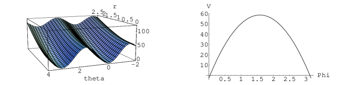
Figure 2: Scalar potential $V$ of $T^{*}{\bf C}P^{1}$ model exhibiting discrete vacua. Left figure gives the potential as a function of two independent variables $r,\theta$. Vacua are located at $(r,\theta)=(0,0),\,(0,\pi)$. The BPS wall solution interpolates these two vacua through the path $r=0$. Right figure shows the potential along the $r=0$ section as a function of $\Phi=\Phi^{1}$. Parameters are taken to be $(g_{0}M^{0},\kappa)=(3,0.1)$, $(\alpha_{1},d_{1,1},d_{1,2})=(10^{-\frac{3}{2}},1,1)$ and $(\alpha_{0},d_{0,1},d_{0,2})=(0,-1,1)$.

The SUSY vacua become local minima of the scalar potential. BPS domain wall which interpolates between these two vacua $(r,\theta)=(0,0)$ and $(0,\pi)$ was obtained as [17], [18]

$$r=0,\quad\cos\theta=\tanh(2g_{0}M^{0}(y-y_{0})),\quad\Theta={\rm const.},$$ (3.60)

and $\Psi$ undetermined. Hence, the wall trajectory runs only on the section $r=0$. Let us turn to our ansatz. Our ansatz (3.39) and (3.41) correspond to the section : $r=0$, $\Theta=2\theta_{1}$ and $\Psi$ undetermined. Therefore our ansatz precisely covers the field space traversed by the domain wall configuration interpolating the two vacua as illustrated in Fig.2.

We note also a simplification for the special case where we choose the symmetric kinetic term $d_{1,a}=d_{1,n+1}$ for the $U(1)$ generator $t_{1}$ as in Eq.(2.19). The BPS equations (3.50) becomes very simple:

$$\partial_{y}\Phi^{a}=\left[\nu_{0,a}-\frac{1}{m}\sum_{b=1}^{n+1}\nu_{0,b}\Phi^{b}\right]\Phi^{a}\quad(a=1,2,\cdots,n+1),$$ (3.61)

and the VEV reduces to $\Phi^{b}=m\delta^{b}{{}_{a}}$. This is the case which was studied extensively in the global SUSY case ($\kappa\rightarrow 0$) previously [13]. The scalar potential also becomes simple:

$$V=\frac{1}{2(1-\kappa^{2}m)}\left[\sum_{b=1}^{n+1}\nu_{0,b}^{2}\Phi^{b}-\frac{1}{m}\left(\sum_{b=1}^{n+1}\nu_{0,b}\Phi^{b}\right)^{2}\right]-\frac{2\kappa^{2}}{3}\left(a+\frac{1}{1-\kappa^{2}m}\sum_{b=1}^{n+1}\nu_{0,b}\Phi^{b}\right)^{2}.$$ (3.62)

The first term is precisely the same as the potential in the global SUSY case except a gravitational correction of the overall factor, whereas the second term gives a genuine gravitational correction. We will study this potential more closely when discussing the weak gravity limit in sect.5.

4 Exact BPS solutions

4.1 General properties

As we showed in sect.3.1, the field space of our BPS solutions is restricted in the $n$ simplex $\Sigma_{1}^{(n)}$ in Eq.(3.26) with the SUSY vacua as their $n+1$ vertices (or subsimplexes for degenerate cases). Our solutions of the BPS equation will be expressed as one-dimensional curves which interpolates between two vertices (or subsimplexes for degenerate cases) of $\Sigma^{(n)}_{1}$. These curves never intersect each other, since these are the solutions of the first order ordinary differential equations.

Let us consider a BPS kink interpolating between two SUSY vacua $c$ and $d$ :

$$\begin{array}[]{l}\Phi^{a}\rightarrow m_{a}\delta^{a}{{}_{c}}\quad{\rm as}\quad y\rightarrow-\infty,\\ \Phi^{a}\rightarrow m_{a}\delta^{a}{{}_{d}}\quad{\rm as}\quad y\rightarrow+\infty.\end{array}$$ (4.3)

Since the variables $\Phi^{a}$ satisfy $\sum_{a}\Phi^{a}/m_{a}=1$ as given in Eq.(3.25) and $\Phi^{a}\geq 0$ by definition, $\Phi^{a\neq c,d}$ must vanish as $y\rightarrow\pm\infty$. Near the two vacua (4.3), the BPS equations (3.50) behave as

$$\begin{array}[]{l}\partial_{y}\Phi^{a}\sim\nu_{1,a}\left(\dfrac{\nu_{0,a}}{\nu_{1,a}}-\dfrac{\nu_{0,c}}{\nu_{1,c}}\right)\Phi^{a}\quad{\rm as}\ y\rightarrow-\infty,\\ \partial_{y}\Phi^{a}\sim\nu_{1,a}\left(\dfrac{\nu_{0,a}}{\nu_{1,a}}-\dfrac{\nu_{0,d}}{\nu_{1,d}}\right)\Phi^{a}\quad{\rm as}\ y\rightarrow+\infty.\end{array}$$ (4.6)

To find out generic features of BPS wall solutions, it is useful to determine ordering of vacua [13]. For general choices of $\alpha_{I}$ and $d_{I,a}$ it is a complicated matter to determine the ordering of the SUSY vacua. For simplicity, we assume that $\nu_{1,a}=2g_{0}M^{0}\left(\alpha_{1}-d_{1,a}\right)<0$ for any $a$. This assumption is always realized in the weak gravity limit where $\alpha_{1}\sim{\cal O}(\kappa^{2})\ll 1$. The above asymptotic behavior of the BPS equations (4.6) suggests that the ordering of vacua should be made with respect to the ratio $\nu_{0,a}/\nu_{1,a}$. Here we assume the ordering of vacua as

$$\dfrac{\nu_{0,1}}{\nu_{1,1}}>\cdots>\dfrac{\nu_{0,n+1}}{\nu_{1,n+1}}.$$ (4.7)

Let us consider the case $c<d$. Combining the asymptotic form (4.6) and the above boundary conditions (4.3), we find that $\Phi^{a}$ with $a<c$ and $a>d$ must vanish identically at any $y$. Therefore we need to consider fields $\Phi^{a}$ for $c\leq a\leq d$. Since $\Phi^{a}$ with $c<a<d$ must vanish as $y\rightarrow\pm\infty$, they have at least one maximum.

For simplicity, we consider the case of symmetric kinetic term $d_{1,a}=d_{1,n+1}$, $a=1,\cdots,n$ as in Eq.(2.19). Ordering of vacua should now be specified by $\nu_{0,1}<\cdots<\nu_{0,n+1}$. If we consider a kink interpolating between $c$-th and $d$-th vacua, we have again nonvanishing fields $\Phi^{a},a=c,\cdots,d$ which now satisfies a simplified BPS equations

$$\partial_{y}\Phi^{a}=\frac{1}{m}\left(\sum_{b=c}^{d}(\nu_{0,a}-\nu_{0,b})\Phi^{b}\right)\Phi^{a},\quad\quad\left(c\leq a\leq d\right).$$ (4.8)

This BPS equation implies that $\Phi^{a=c,d}$ is monotonic functions of $y$. Then we find that the curves which interpolate between $c$-th and $d$-th vacua is embedded in the $\ell=d-c$ subsimplex $\sigma^{(l)}_{1}$ in $\Sigma^{(n)}_{1}$. Therefore it is enough to consider solutions which interpolate between the first and the last vacuum. This embedding of multi-wall solutions in the subsimplexes is an extension of a feature already noted in the global SUSY model with the symmetric kinetic term in Ref.[13].

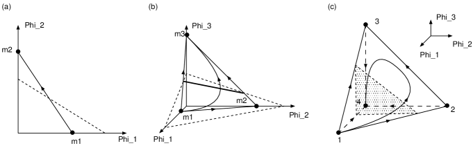
Figure 3: Solution space for $n=1,2,3$. Solid lines express the simplex $\Sigma_{1}^{(n)}$ and broken lines denote $\Sigma_{0}^{(n)}$. The curves in $\Sigma_{1}^{(n)}$ denotes the solution curve.

One of the advantages of using the geometrical picture in terms of $\Phi^{a}$ is that we can obtain the information about the warp factor very easily. In four-dimensional SUGRA [6, 7] or the $D$-dimensional effective SUGRA [28, 46], the killing spinor equations are obtained:

$$\partial_{y}\phi^{i}(y)=C_{D}\frac{\partial W(\phi^{i})}{\partial\phi^{i}},\quad\partial_{y}U(y)=-\kappa^{2}C^{\prime}_{D}W(\phi^{i}),$$ (4.9)

where $C_{D}$ and $C^{\prime}_{D}$ are positive constants which depend on spacetime dimension $D$. A real function $W$ is called “superpotential”. Therefore, necessary and sufficient condition for the presence of the stationary point of the warp factor is given by the existence of zero of the “superpotential” along the wall trajectory. From Eq.(4.9) we obtain

$$\partial_{y}^{2}U=-\kappa^{2}C_{D}C^{\prime}_{D}\sum_{i}\left(\dfrac{\partial W}{\partial\phi^{i}}\right)^{2}\leq 0.$$ (4.10)

Since $\partial_{y}^{2}U$ is non-positive definite, $\partial_{y}U$ is always a monotonic function, and the warp factor has at most a single stationary point. Eq.(4.9) shows that the warp factor can vanish at both infinity resulting in a space-time regular in the entire bulk, if the superpotential $W$ has odd numbers of zeroes along the wall trajectory. On the contrary, if the superpotential has no zero at all (or even numbers of zeros), the warp factor is singular at least at either one side of the wall. In that case, the BPS wall solution expresses the coupling flow of certain four-dimensional field theory according to the AdS/CFT correspondence.

Let us introduce “superpotential” for our model. We define it as a derivative of the function $U$ in the warp factor in Eq.(3.40):

$$\partial_{y}U=-\frac{\kappa^{2}}{3}(2g_{0}M^{0}\bar{\cal A}^{-1}{\cal T}_{0})\equiv-\frac{\kappa^{2}}{3}W.$$ (4.11)

Here, we impose the constraint ${\cal T}_{1}=0$. We will discuss the superpotential $W$ in some detail in Appendix B. The warp factor has a stationary point at a point where $W=0$. The condition $W=0$ leads to ${\cal T}_{0}=0$ from its definition (4.11). This ${\cal T}_{0}=0$ condition defines a hyperplane which we shall call $\Sigma_{0}^{(n)}$. We also denote the intersection of $\Sigma_{1}^{(n)}$ and $\Sigma_{0}^{(n)}$ as $\Omega^{(n-1)}$. The $\partial_{y}U$ vanishes on the intersection $\Omega^{(n-1)}$. This means that the warp factor does not have a stationary point when $\Sigma_{1}^{(n)}$ and $\Sigma_{0}^{(n)}$ do not intersect each other. On the other hand, there exist some stationary points of $W$, if the $\Sigma_{0}^{(n)}$ and $\Sigma_{1}^{(n)}$ intersect. The number of the stationary points of $W$ equals to the number of intersections between the trajectory and $\Omega^{(n-1)}$. The warp factor increases (decreases) in the lower (upper) half space below (above) the hyperplane $\Sigma^{(n)}_{0}$ along the wall trajectory. We show this circumstance in Fig.3 for $n=1,2,3$. At this stage we have a question whether the wall trajectory can have two or more intersections with $\Omega^{(n-1)}$. It is familiar that $\partial_{y}^{2}U<0$ around a positive energy density which comes from the wall tension or the localized positive brane tension. On the other hand, $\partial_{y}^{2}U>0$ can be realized only if there exists a localized artificial negative energy density [2]. This physical argument suggests that the wall trajectory can have at most one intersecting point with $\Omega^{(n-1)}$. We can prove this explicitly in the case of the symmetric kinetic term ($d_{1,a}=d_{1,n+1}$ for any $a$). For this case the BPS equation for the matter field can be expressed as, (see Appendix B)

$$\partial_{y}\varphi^{a}=\frac{1}{4}\frac{\partial W}{\partial\varphi^{a}},\qquad{\rm where}\quad\Phi^{a}=(1-\kappa^{2}m_{a})(\varphi^{a})^{2}.$$ (4.12)

Combining this with Eq.(4.11), we find

$$\partial_{y}^{2}U=-\frac{\kappa^{2}}{12}\sum_{b=1}^{n+1}\left(\frac{\partial W}{\partial\varphi^{b}}\right)^{2}<0.$$ (4.13)

Hence, the warp factor also has at most a single stationary point for our model at least in the case of symmetric kinetic term.

4.2 Exact solutions

4.2.1 generalized $QT^{*}{\bf C}P^{n}$ (asymmetric kinetic term)

First we will consider the BPS solutions for generalized $QT^{*}CP^{n}$ models whose kinetic terms are not symmetric ($d_{1a}\not=d_{1b}$, $a\not=b$). To obtain an exact BPS solutions, we rewrite Eq.(3.50) as follows:

$$\frac{1}{\nu_{1,a}}\frac{\partial_{y}\Phi^{a}}{\Phi^{a}}=\frac{\nu_{0,a}}{\nu_{1,a}}+f(\Phi).$$ (4.14)

We can eliminate a complicated, but an $a$ independent quantity $f(\Phi)$ by subtracting ($n+1$)-th equation

$$\frac{1}{\nu_{1,a}}\frac{\partial_{y}\Phi^{a}}{\Phi^{a}}-\frac{1}{\nu_{1,n+1}}\frac{\partial_{y}\Phi^{n+1}}{\Phi^{n+1}}=\frac{\nu_{0,a}}{\nu_{1,a}}-\frac{\nu_{0,n+1}}{\nu_{1,n+1}}.$$ (4.15)

Then we can express $\Phi^{a}$ by $\Phi^{n+1}$ for $a=1,2,\cdots,n$:

$$\Phi^{a}=\left(\Phi^{n+1}\right)^{\frac{\nu_{1,a}}{\nu_{1,n+1}}}\ \exp\left[\nu_{1,a}\left(\frac{\nu_{0,a}}{\nu_{1,a}}-\frac{\nu_{0,n+1}}{\nu_{1,n+1}}\right)(y-y_{a})\right],$$ (4.16)

where $y_{a}$ is an integration constant. Plugging this into the constraint (3.25), $\Phi^{n+1}$ is implicitly obtained as a function of $y$:

$$1=\sum_{b=1}^{n+1}\frac{1}{m_{b}}\left(\Phi^{n+1}\right)^{\frac{\nu_{1,b}}{\nu_{1,n+1}}}\ \exp\left[\nu_{1,b}\left(\frac{\nu_{0,b}}{\nu_{1,b}}-\frac{\nu_{0,n+1}}{\nu_{1,n+1}}\right)(y-y_{b})\right].$$ (4.17)

Pulling this back into Eq.(4.16), we can also obtain $\Phi^{a}$ as a function of $y$. The superpotential $W$ in Eq.(4.11) is given by

$$W=a+\frac{\displaystyle\sum_{b=1}^{n+1}\nu_{0,b}\Phi^{b}}{\displaystyle\sum_{b=1}^{n+1}\dfrac{1-\kappa^{2}m_{b}}{m_{b}}\Phi^{b}},$$ (4.18)

with the parameter $a$ defined in Eq.(3.52). The BPS equation of the function $U$ in the warp factor is given by Eq.(4.11) with the above superpotential. Ignoring the irrelevant integration constant of the warp factor, we obtain :

$$U=-\frac{\kappa^{2}}{3}\ ay-\frac{\kappa^{2}}{3}\int dy\ \left(\frac{\displaystyle\sum_{b=1}^{n+1}\nu_{0,b}\Phi^{b}}{\displaystyle\sum_{b=1}^{n+1}\dfrac{1-\kappa^{2}m_{b}}{m_{b}}\Phi^{b}}\right).$$ (4.19)

Eqs.(4.16), (4.17), and (4.19) constitute the full set of our exact BPS solutions of multi-walls. One should note that the above derivation does not rely on whether there are vacuum degeneracy or not. Therefore the above set of solutions is valid, irrespective of vacua being degenerate or nondegenerate.

The parameter $a$ in Eq.(4.19) determines the behavior of the function $U$ in the warp factor at infinity [31]. Since $m_{1}\nu_{0,1}/(1-\kappa^{2}m_{1})\leq m_{n+1}\nu_{0,n+1}/(1-\kappa^{2}m_{n+1})$ because of the vacuum ordering, we have only three possible types of asymptotic behaviors with respect to the AdS/CFT correspondence [37]: UV-IR, IR-flat, IR-IR. If $0<a+m_{1}\nu_{0,1}/(1-\kappa^{2}m_{1})$, we have an ultraviolet (UV) vacuum at $y\rightarrow-\infty$, and an infrared (IR) vacuum at $y\rightarrow\infty$. If $a+m_{1}\nu_{0,1}/(1-\kappa^{2}m_{1})=0$, we have a flat Minkowski space at $y\rightarrow-\infty$, and an IR vacuum at $y\rightarrow\infty$. If $a+m_{1}\nu_{0,1}/(1-\kappa^{2}m_{1})<0<a+m_{n+1}\nu_{0,n+1}/(1-\kappa^{2}m_{n+1})$, we have an IR vacuum at $y\rightarrow-\infty$, and an IR vacuum at $y\rightarrow\infty$. If $a+m_{n+1}\nu_{0,n+1}/(1-\kappa^{2}m_{n+1})=0$, we have an IR vacuum at $y\rightarrow-\infty$, and a flat Minkowski space at $y\rightarrow\infty$. If $a+m_{n+1}\nu_{0,n+1}/(1-\kappa^{2}m_{n+1})<0$, we have an UV vacuum at $y\rightarrow-\infty$, and an IR vacuum at $y\rightarrow\infty$.

Our solutions contain $n$ real parameters, $(y_{1},y_{2},\cdots,y_{n})$. They corresponds to the $n$ collective coordinates discovered in the BPS multi-wall solutions of $T^{*}{\bf C}P^{n}$ models with global SUSY [13]. In the case of nondegenerate vacua, they are related to the locations of $n$ walls at least for large positive separation between them. If there are degenerate vacua, the parameters associated with these degenerate vacua actually reduces to the moduli parameters of the degenerate vacua. We shall see both these points more explicitly for the model with symmetric kinetic terms below. In the $T^{*}{\bf C}P^{n}$ model with global SUSY, there are also $n$ moduli coming from the spontaneously broken internal $U(1)^{n}_{\rm F}$ flavor symmetries in addition to the $n$ moduli of the wall locations [13]. Our model also has these $U(1)^{n}_{\rm F}$ flavor symmetries which are broken spontaneously. This point can be seen by the freedom to choose the phase $\theta_{a}$ of our solution $\phi_{1}{{}^{a}}$, $a=1,\cdots,n+1$ in Eq.(3.41). At a glance, there appear to be $n+1$ additional moduli parameters. In our model with SUGRA, however, we have two $U(1)$ directions $t_{1},t_{0}$ which are locally gauged. Therefore phase rotations along these directions can be gauged away and unphysical. The phase rotation with $\theta_{a}=d_{1,a}\theta\ (a=1,2,\cdots,n+1)$ is gauged by $t_{1}$ and is absorbed into gauge field $W_{\mu}^{1}$. Another phase rotation with $\theta_{a}=d_{0,a}\theta$ is gauged by $t_{0}$ and is absorbed into gauge field $W_{\mu}^{0}$. Therefore, the number of the physical parameters associated with the internal flavor symmetries are $n-1$. Therefore the number of the massless scalar fields associated with the phase rotations is less by one than the global SUSY model. In the weak gravity limit, the scalar field absorbed by the central charge vector multiplet $W_{\mu}^{0}$ is recovered, since the gauge coupling $g_{0}$ should vanish and the associated gauge symmetry becomes global symmetry as $\kappa\rightarrow 0$.

Similarly to the phase rotations, there are $n$ parameters $y_{a},a=1,\cdots,n$ corresponding to the locations of the walls in the global SUSY model without gravity. Therefore there are $n$ real parameters (collective coordinates) in the solution. In the presence of gravity, the center of mass coordinate is gauged away, since the gravity can be understood as a gauge theory for translation symmetry. In fact, we have recently shown in a similar SUGRA model in the four-dimensional spacetime [50] that the scalar fluctuations in the Newton gauge have a zero mode which can however be gauged away and unphysical. Moreover this mode turned out to become the Nambu-Goldstone mode in the limit of vanishing gravitational coupling [50]. Consequently, the physical parameters of the BPS solution in our model with SUGRA should be $n-1$ $U(1)$ phases and $n-1$ relative distances of walls, which will eventually form $n$ complex massless fields in accord with the remaining ${\cal N}=1$ SUSY.

4.2.2 $QT^{*}{\bf C}P^{n}$ model (symmetric kinetic term)

In the case of symmetric kinetic term ($d_{1,1}=\cdots=d_{1,n+1}$), it is most convenient to use the parameters

$$\mu_{a}\equiv\nu_{0,n+1}-\nu_{0,a}.$$ (4.20)

instead of $\nu_{0,a}$. In this case, we can simplify our solution for $\Phi^{a}$. Eq.(4.17) can be inverted explicitly to give

$$\Phi^{n+1}(y)=\frac{m}{\displaystyle\sum_{b=1}^{n+1}{\rm e}^{-\mu_{b}(y-y_{b})}}.$$ (4.21)

Eq.(4.16) can also be solved explicitly to give :

$$\Phi^{a}(y)=\frac{m{\rm e}^{-\mu_{a}(y-y_{a})}}{\displaystyle\sum_{b=1}^{n+1}{\rm e}^{-\mu_{b}(y-y_{b})}},\quad\left(a=1,2,\cdots,n\right).$$ (4.22)

The function $U$ in the warp factor in Eq.(4.19) is given more explicitly by

$$U=-\frac{\kappa^{2}}{3}\left[\tilde{a}y+\frac{m}{1-\kappa^{2}m}\log\left(\sum_{b=1}^{n+1}{\rm e}^{-\mu_{b}(y-y_{b})}\right)\right]$$ (4.23)

where $\tilde{a}\equiv a+m\nu_{0,n+1}(1-\kappa^{2}m)^{-1}$ with $a$ defined in (3.52). This warp factor for $n$ nondegenerate vacua consists of $n+1$ regions with different values of derivatives at least for large separations between $n$ walls. These solutions (4.22) and (4.23) are valid irrespective of vacuum degeneracy. However, the physical meaning of the parameters $y_{a},\;a=1,\cdots,{n+1}$ is clearest in the case of nondegenerate vacua. At least for large positive separation, these parameters have an intuitive physical meaning as the locations of boundaries between vacua $a$ and $n+1$ as we shall see below. On the other hand, the parameter $\mu_{a}$ yields the inverse width of each wall associated with $y_{a}$. More precise identification will be made by taking $n=2,3$ as illustrative examples below.

We can rewrite the above solutions (4.21) and (4.22) for the case of degenerate vacua, to clarify the meaning of the parameter $y_{a}$ for degenerate vacua. Let us assume that the $\ell+1$ vacua $a,a+1,\cdots,a+\ell$ are degenerate and all the other vacua are nondegenerate. As we have seen in sect.3.1, these degenerate vacua correspond to $\ell$ subsimplex $\sigma^{(\ell)}_{1}$ of $\Sigma^{(n)}_{1}$. If vacua at $y=\pm\infty$ are $a=I$ and $a=F$, all fields $\Phi^{a}$ with $a<I$ and $F<a$ vanish identically. Therefore we shall consider the multi-wall solution interpolating between the first $a=1$ and the last vacua $a=n+1$, without loss of generality. Consequently the multi-wall solution comes close to (or starts at, or ends at) the degenerate vacuum subsimplex $\sigma^{(\ell)}_{1}$. From the BPS equation, we find

$$\frac{\partial_{y}\Phi^{a}}{\Phi^{a}}=\frac{\partial_{y}\Phi^{a+1}}{\Phi^{a+1}}=\cdots=\frac{\partial_{y}\Phi^{a+\ell}}{\Phi^{a+\ell}}.$$ (4.24)

This implies that the solution is embedded in an $(n-\ell)$-dimensional hypersurface inside the simplex $\Sigma^{(n)}_{1}$ defined as

$$\Phi^{a}=k_{a}\tilde{\Phi}^{a},\quad\Phi^{a+1}=k_{a+1}\tilde{\Phi}^{a},\cdots,\Phi^{a+\ell}=k_{a+\ell}\tilde{\Phi}^{a},$$ (4.25)

$$\tilde{\Phi}^{a}\equiv\Phi_{a}+\cdots+\Phi_{a+\ell}.$$ (4.26)

where $k_{a},\dots,k_{a+\ell}$ are arbitrary positive constants constrained by $k_{a}+\cdots+k_{a+\ell}=1.$

This shows that the relative amount $k_{b}$ of fields $\Phi^{b}$ compared to the sum of fields associated to the degenerate vacua are constant. The remaining procedure for obtaining the solution is completely the same as above nondegenerate case. We find that the multi-wall solution for the $\ell+1$ degenerate vacua is exactly the same as the multi-wall solution for the case of $QT^{*}{\bf C}P^{n-\ell}$ model, with one of the field being the sum of these fields with degenerate vacua $\tilde{\Phi}^{a}$.

$$\tilde{\Phi}^{a} = {\rm e}^{-\mu_{a}(y-y_{a})}\Phi^{n+1},$$ (4.27)

$$\Phi^{b} = {\rm e}^{-\mu_{b}(y-y_{b})}\Phi^{n+1},\quad(b=1,\cdots,a-1,a+\ell+1,\cdots,n+1).$$ (4.28)

Plugging this into the constraint $\displaystyle\sum_{b-1}^{n+1}\Phi^{b}=m$, we obtain

$$\Phi^{n+1}=\frac{m}{\displaystyle\sum_{b=1}^{a-1}{\rm e}^{-\mu_{b}(y-y_{b})}+{\rm e}^{-\mu_{a}(y-y_{a})}+\sum_{b=a+\ell+1}^{n+1}{\rm e}^{-\mu_{b}(y-y_{b})}}.$$ (4.29)

We see that the parameters $y_{a},\cdots,y_{a+\ell}$ in the general solutions (4.16) and (4.17) are transformed into these relative amount $k_{a}$ and $y_{a}$ associated to the location of the wall. Clearly the field space for this degenerate vacua is isomorphic to the field space $\Sigma_{1}^{(n-\ell)}$ for the $QT^{*}{\bf C}P^{n-\ell}$ model. The function $U$ in the warp factor is also given by (4.23) with the sum of the fields associated with the degenerate vacua replaced by $\tilde{\Phi}^{a}$.

It is now obvious how to generalize the above result to more involved situation with arbitrary numbers of groups of degenerate vacua together with nondegenerate vacua. We shall illustrate below these cases in explicit solutions for $n=2$ and $3$.

4.2.3 $n=2$ case ($QT^{*}{\bf C}P^{2}$)

Here we deal with the $n=2$ case in some detail. For simplicity, we consider the case of the symmetric kinetic term ($d_{1,a}=d_{1,n+1}$ for any $a$) in the remainder of this section. Let us first take nondegenerate case. The SUSY vacuum structure and the scalar potential are illustrated in Fig.4.

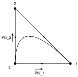
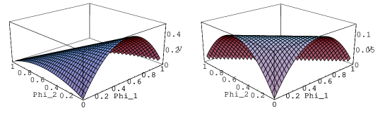
Figure 4: SUSY vacua and a wall trajectory are expressed in the left figure. Scalar potential $V$ as a function of independent fields $\Phi^{1},\Phi^{2}$ in the middle and right figure. The middle has $\mu_{1}=2\neq\mu_{2}=1$ (asymmetric kinetic term) and the right has $\mu_{1}=\mu_{2}=1$ (symmetric kinetic term). In both figures $m=1,\kappa=0.1$.

Notice that $\mu_{1}>\mu_{2}>0$ from the above vacuum ordering (4.7). The general two wall solution is given by :

$$\Phi^{1} = \dfrac{m\ {\rm e}^{-\mu_{1}(y-y_{1})}}{1+{\rm e}^{-\mu_{1}(y-y_{1})}+{\rm e}^{-\mu_{2}(y-y_{2})}}=\frac{m}{1+{\rm e}^{\mu_{1}(y-y_{1})}+{\rm e}^{(\mu_{1}-\mu_{2})(y-y_{12})}},$$ (4.30)

$$\Phi^{2} = \dfrac{m\ {\rm e}^{-\mu_{2}(y-y_{2})}}{1+{\rm e}^{-\mu_{1}(y-y_{1})}+{\rm e}^{-\mu_{2}(y-y_{2})}}=\frac{m}{1+{\rm e}^{\mu_{2}(y-y_{2})}+{\rm e}^{-(\mu_{1}-\mu_{2})(y-y_{12})}},$$ (4.31)

$$\Phi^{3} = \dfrac{m}{1+{\rm e}^{-\mu_{1}(y-y_{1})}+{\rm e}^{-\mu_{2}(y-y_{2})}}.$$ (4.32)

where we define the separation $y_{ab}$ between vacua $a$ and $b$ as

$$y_{ab}\equiv\dfrac{\mu_{a}}{\mu_{a}-\mu_{b}}y_{a}-\frac{\mu_{b}}{\mu_{a}-\mu_{b}}y_{b},\qquad y_{ab}=y_{ba},$$ (4.33)

with the understanding that $y_{a}\equiv y_{a,n+1}$ ($n=2$ in our case). The parameter $y_{ab}$ has a physical meaning of the location of the boundary between the vacua $a$ and $b$. If these two vacua are adjacent, it in fact becomes the location of the wall separating these two vacua. Here, $\Phi^{3}$ is not an independent field because of the constraint $\Phi^{1}+\Phi^{2}+\Phi^{3}=m$.

Figure 5: Two-wall solutions for $n=2$ nondegenerate case : $y_{12}$ goes through $y_{2}$ from left to right. Parameters are taken to be $m=1$, and $(\mu_{1},\mu_{2})=(2,1)$, and $(y_{1},y_{2})=(0,10),(0,2),(0,-10)$ from left to right.

Figure 6: The functions $U$ in the warp factor corresponding to the solutions in Fig.5. Parameters are taken to be $\kappa=0.1$, $\tilde{a}=0.5$, $m=1$, and $(\mu_{1},\mu_{2})=(2,1)$, and $(y_{1},y_{2})=(0,10),(0,2),(0,-10)$ from left to right.

The solution shows that $\Phi^{1}\rightarrow m,$ and $\Phi^{2},\Phi^{3}\rightarrow 0$ as $y\rightarrow-\infty$, and $\Phi^{1},\Phi^{2}\rightarrow 0$ and $\Phi^{3}\rightarrow m$ as $y\rightarrow\infty$. If we wish to see the region of vacuum $2$ appearing clearly, we should arrange the parameters such that $y_{1}<y_{2}$. Then the ordering becomes

$$y_{12}<y_{1}\equiv y_{13}<y_{2}\equiv y_{23}.$$ (4.34)

Hence, $\Phi^{1}$ has a wall behavior centered around $y=y_{12}$, and $\Phi_{2}$ has two walls at the vicinity of $y_{12}$ and $y_{2}$, ($\Phi^{3}$ has a wall centered around $y_{2}$) as illustrated in the left-most of Fig.5. The corresponding solutions of the function $U$ in the warp factor in Eq.(4.23) are shown in Fig.6. Three separate regions are clearly visible in the left-most of Fig.6. In the right-most of Fig.6, a sharp turn-over of $U$ coresponds to small (almost invisible) $\Phi^{2}$ in the right-most of Fig.5.

The relative distance $R$ between these two walls is given as

$$R\equiv y_{2}-y_{12}=\frac{\mu_{1}}{\mu_{1}-\mu_{2}}(y_{2}-y_{1}).$$ (4.35)

When $y_{2}$ approaches to $y_{1}$, the two walls are compressed each other. If $y_{2}$ becomes smaller than $y_{1}$, $R$ loses the intuitive physical meaning of the relative distance. It is still a parameter of the solution which has an interesting nontrivial dynamics [14], [16]. We illustrate the behavior of multi-wall solution as $y_{12}$ goes through $y_{2}$ from left to right in Fig.5. The above explicit solutions (4.32) satisfy [13]

$$(\Phi^{1})^{\mu_{2}}(\Phi^{2})^{-\mu_{1}}(\Phi^{3})^{\mu_{1}-\mu_{2}}={\rm e}^{-\mu_{2}(\mu_{1}-\mu_{2})R}.$$ (4.36)

Hence, the relative distance $R$ determines the trajectory of the solution curve in $\Sigma^{(2)}_{1}$, and the center of mass coordinate $y_{\rm cm}\equiv(y_{12}+y_{2})/2$ determines the mapping from the base space $y$ to the trajectory in $\Sigma^{(2)}_{1}$. When $R$ becomes zero or negative, two walls are compressed each other and the solution curves are close to the straight line (subsimplex $\sigma^{(1)}_{1}$) connecting the first and the last vacua. In the limit of $R\rightarrow-\infty$, it should reduce to the so-called fundamental wall [13] connecting the first and the last vacua directly without exciting $\Phi^{2}$ at all. As $R(>0)$ grows, the corresponding solution curve goes closer to the vacuum $2$. If we take $R$ infinity, two far away walls approach the two fundamental walls, each of which corresponds to the $1\rightarrow 2$ and $2\rightarrow 3$ wall, respectively.

Figure 7: Solution for $n=2$ degenerate case. Parameters are taken to be $m=1,\mu_{1}=1,y_{1}=0$.

Next we turn to degenerate case with $d_{0,1}=d_{0,2}$ ($d_{1,1}=d_{1,2}=d_{1,3}$). In this case we have an isolated vacuum $(\Phi^{b}=m\delta^{b}{{}_{3}})$ and a degenerate vacuum which is represented by a subsimplex $\sigma^{(1)}_{1}$ with the vacua $1,2$ as its vertex. The BPS solutions are given by :

$$\tilde{\Phi}^{1}(y) \!\!\!= \!\!\!\frac{m{\rm e}^{-\mu_{1}(y-y_{1})}}{1+{\rm e}^{-\mu_{1}(y-y_{1})}}=\frac{m}{{\rm e}^{\mu_{1}(y-y_{1})}+1},$$ (4.37)

$$\Phi^{3}(y) \!\!\!= \!\!\!\frac{m}{1+{\rm e}^{-\mu_{1}(y-y_{1})}},$$ (4.38)

$$\Phi^{1}(y) \!\!\!= \!\!\!k_{1}\tilde{\Phi}^{1}(y),\qquad\Phi^{2}(y)=k_{2}\tilde{\Phi}^{1}(y),\qquad k_{1}+k_{2}=1.$$ (4.39)

The solution has two parameters : $y_{1}$ and $k_{1}=1-k_{2}$. The parameter $y_{1}$ corresponds to the position of the wall and $k_{1}$ is the relative amount of the field $\Phi^{1}$ within $\tilde{\Phi}^{1}$ associated to the degenerate vacuum. The field space and the solution in the case of the degenerate vacua is illustrated in Fig.7.

4.2.4 $n=3$ case ($QT^{*}{\bf C}P^{3}$)

Here we work out the $n=3$ case in some detail. We shall consider the case of the symmetric kinetic term $d_{1,1}=d_{1,2}=d_{1,3}=d_{1,4}$. Writing out three independent fields only, we obtain the three wall solution as :

$$\Phi^{1} = \frac{m}{1+{\rm e}^{\mu_{1}(y-y_{1})}+{\rm e}^{(\mu_{1}-\mu_{2})(y-y_{12})}+{\rm e}^{(\mu_{1}-\mu_{3})(y-y_{13})}},$$ (4.40)

$$\Phi^{2} = \frac{m}{1+{\rm e}^{\mu_{2}(y-y_{2})}+{\rm e}^{(\mu_{2}-\mu_{3})(y-y_{23})}+{\rm e}^{-(\mu_{1}-\mu_{2})(y-y_{12})}},$$ (4.41)

$$\Phi^{3} = \frac{m}{1+{\rm e}^{\mu_{3}(y-y_{3})}+{\rm e}^{-(\mu_{1}-\mu_{3})(y-y_{13})}+{\rm e}^{-(\mu_{2}-\mu_{3})(y-y_{23})}},$$ (4.42)

where we used the variable $y_{ab}$ defined in Eq.(4.33). Notice that $y_{ab}$ are not fully independent, and satisfy the identity such as :

$$(\mu_{1}-\mu_{2})y_{12}+(\mu_{2}-\mu_{3})y_{23}+(\mu_{3}-\mu_{1})y_{31}=0.$$ (4.43)

If we wish to have the region of vacuum $2$ and $3$ clearly visible, we should arrange the parameters $y_{12}<y_{23}<y_{3}$. Then we automatically obtain the ordering

$$y_{12}<y_{13}<y_{23}<y_{2}(=y_{24})<y_{3}(=y_{34}).$$ (4.44)

Provided these relative distances are large and positive, $y_{12}$, $y_{23}$ and $y_{3}$ have an intuitive physical meaning of the location of the left (vacuum$1\rightarrow$ vacuum$2$) wall, the middle (vacuum$2\rightarrow$ vacuum$3$) wall, and the right (vacuum$3\rightarrow$ vacuum$4$) wall. Then the relative distances between two adjacent walls can be defined as

$$R_{12}=y_{23}-y_{12},\quad R_{23}=y_{3}-y_{23}.$$ (4.45)

A typical three wall solution for nondegenerate case is shown in Fig.8.

Figure 8: Solution for $n=3$ nondegenerate case. Parameters are taken to be $m=1$, $(\mu_{1},\mu_{2},\mu_{3})=(3,2,1)$ and $(y_{1},y_{2},y_{3})=(0,10,20)$.

Next we turn to the degenerate case. Compared to the $n=2$ case, we have more varieties of degenerate cases. Since there are four possible vacua, there can be degeneracies among two, three, and four vacua. The case of four degenerate vacua does not give wall solution. The case of three degenerate vacua can occur either for the first three vacua $(1,2,3)$ or the last three vacua $(2,3,4)$. The case of two degenerate vacua can occur either between the first two vacua $(1,2)$, or the last two vacua $(3,4)$, or the middle two vacua $(2,3)$. Consequently we can have two groups of degenerate vacua $(1,2)$ and $(3,4)$. We shall illustrate these typical solutions in the following.

If the last two vacua $(3,4)$ are degenerate and the rest are nondegenerate, we obtain

$$\Phi^{1} = \frac{m}{1+{\rm e}^{\mu_{1}(y-y_{1})}+{\rm e}^{(\mu_{1}-\mu_{2})(y-y_{12})}},$$ (4.46)

$$\Phi^{2} = \frac{m}{1+{\rm e}^{\mu_{2}(y-y_{2})}+{\rm e}^{-(\mu_{1}-\mu_{2})(y-y_{12})}},$$ (4.47)

$$\tilde{\Phi}^{3} \equiv \Phi^{3}+\Phi^{4}=\dfrac{m}{1+{\rm e}^{-\mu_{1}(y-y_{1})}+{\rm e}^{-\mu_{2}(y-y_{2})}},$$ (4.48)

$$\Phi^{3} = k_{3}\tilde{\Phi}^{3},\qquad\Phi^{4}=k_{4}\tilde{\Phi}^{3},\qquad k_{3}+k_{4}=1.$$ (4.49)

This is the two-wall solution which is the same as that in Eq.(4.32) for the $QT^{*}{\bf C}P^{2}$ model, except that the field $\Phi^{3}$ in Eq.(4.32) is now replaced by $\tilde{\Phi}^{3}$, and the ratio $k_{3}/k_{4}=k_{3}/(1-k_{3})$ of the two fields $\Phi^{3}/\Phi^{4}$ is another parameter of the solution. This case is illustrated in Fig.9(a). The case of first two vacua being degenerate is very similar. If the middle two vacua are degenerate, we can use the same solution for $QT^{*}{\bf C}P^{2}$ in Eq.(4.32) by replacing the middle field $\Phi^{2}$ with the sum of the fields $\tilde{\Phi}^{2}\equiv\Phi^{2}+\Phi^{3}$ associated to the degenerate vacua and the last field by $\Phi^{4}$. The ratio $k_{2}/k_{3}=k_{2}/(1-k_{2})$ of these two fields $\Phi^{2}/\Phi^{3}$ is another parameter of the solution. The wall trajectory in field space is similar to Fig.9(a).

If the last three vacua ($2,3,4$) are degenerate, we obtain a single wall solution

$$\Phi^{1} = \dfrac{m\ }{1+{\rm e}^{\mu_{1}(y-y_{1})}},$$ (4.50)

$$\tilde{\Phi}^{2} \equiv \Phi^{2}+\Phi^{3}+\Phi^{4}=\dfrac{m\ }{1+{\rm e}^{-\mu_{1}(y-y_{1})}},$$ (4.51)

$$\Phi^{2} = k_{2}\tilde{\Phi}^{2},\quad\Phi^{3}=k_{3}\tilde{\Phi}^{2},\quad\Phi^{4}=k_{4}\tilde{\Phi}^{2},\quad k_{2}+k_{3}+k_{4}=1.$$ (4.52)

This solution is the same as that in Eq.(4.32) for the $QT^{*}{\bf C}P^{2}$ model with $\tilde{\Phi}^{2}$ replacing $\Phi^{2}$. The relative amount $k_{a}$ of $\Phi^{a}$ in $\tilde{\Phi}^{2}$ are another parameter of the solution. This case is illustrated in Fig.9(b). The case of last three vacua being degenerate is very similar.

Another interesting case is the two groups of degenerate vacua $(1,2)$ and $(3,4)$. We obtain a single wall solution with $\tilde{\Phi}^{1}$ replacing $\Phi^{1}$ and $\tilde{\Phi}^{3}$ replacing $\tilde{\Phi}^{2}$ in the above solution (4.52). The relative amount $k_{a}$ of $\Phi^{a}$ in $\tilde{\Phi}^{2}$ are also the parameters of the solution

$$\Phi^{1}=k_{1}\tilde{\Phi}^{1},\quad\Phi^{2}=k_{2}\tilde{\Phi}^{1},\quad k_{1}+k_{2}=1,\qquad\Phi^{3}=k_{3}\tilde{\Phi}^{3},\quad\Phi^{4}=k_{4}\tilde{\Phi}^{3},\quad k_{3}+k_{4}=1.$$ (4.53)

This case is illustrated in Fig.9(c).

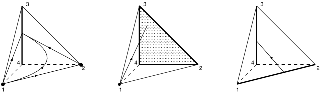
Figure 9: Solution for $n=3$ degenerate case

5 Discussion

Let us first discuss weak gravity limit. In taking the limit, we demand that meaningful models are obtained with the global SUSY. As we noted, we should fix $g_{0}M^{0}$ and $\alpha_{0}/\kappa^{2}$ and $\alpha_{1}/\kappa^{2}$ when taking the limit of vanishing gravitational coupling $\kappa\rightarrow 0$ [31]. By taking this limit with the symmetric kinetic term, we can recover the global SUSY model with the target space $T^{*}{\bf C}P^{n}$ which was studied before in lower dimensions [13]. In this limit, BPS equations for scalar fields in the hypermultiplets reduce to those already studied before [13].

Therefore the model and the solution we discuss in this paper are consistent gravitational deformation of the massive $T^{*}{\bf C}P^{n}$ nonlinear sigma model in five dimensions and associated BPS wall solutions. It is very interesting that BPS solution for the hypermultiplet $\phi$ in the global SUSY model coincides with that in the corresponding SUGRA. This mysterious coincidence was noted in the case of massive Eguchi-Hanson ($T^{*}{\bf C}P^{1}$) nonlinear sigma model [31]. This situation has also appeared in the analytic solution in a four-dimensional ${\cal N}=1$ SUGRA model [7]. It is tempting to speculate that this property might be related to the exact solvability of our model in SUGRA.

For a long time, it has been a difficult problem to find a consistent gravitational deformation from a hyper-Kähler manifold to a quaternionic Kähler manifold with gravitationally corrected potential terms necessary for wall solutions. This goal has been achieved here by using an off-shell formulation of SUGRA and the massive quaternionic Kähler quotient method [31]. There has been an extensive studies of domain walls in SUGRA theories, using the on-shell formulation such as in Ref.[34]. In principle, it may be possible to obtain BPS solutions using the on-shell formulation, since auxiliary fields are eliminated when we solve the BPS equations. However, off-shell formulation of SUGRA provides a more powerful tool to obtain SUGRA domain walls as gravitational deformations of those in global SUSY models. If we eliminate constraints before coupling to gravity, target manifold of nonlinear sigma models are fixed already. Then it is very difficult in general to find out necessary gravitational corrections to the target manifold in order to extend hyper-Kähler nonlinear sigma models with global eight SUSY to quaternionic Kähler nonlinear sigma models coupled to SUGRA. On the other hand, many hyper-Kähler sigma models can be obtained as quotients of linear sigma models by using vector multiplets as Lagrange multipliers [41], [44], [17], [18]. We can first couple these system of gauged linear sigma models to SUGRA before eliminating the Lagrange multiplier multiplets. When we eliminate the Lagrange multipliers after coupling to gravity in the off-shell formulation, we obtain quaternionic Kähler nonlinear sigma models coupled to SUGRA automatically. In this framework, we can take a weak gravity limit of these models straightforwardly. Therefore the off-shell formulation of SUGRA is very useful to obtain quaternionic nonlinear sigma models as continuous gravitational deformations of hyper-Kähler nonlinear sigma models of the global SUSY.

By construction, our models should have quaternionic Kähler target manifold as far as local properties are concerned. However, we have not yet studied possible global obstructions which might exist in these target manifold. We still have to work out the coordinates that parametrize the manifold globally. This is a problem to be studied in future.

At least in the case of $T^{*}{\bf C}P^{1}$ model, it has been noted that our quaternionic manifold has a conical singularity at $r=0$ in $r,\Psi$ plane [31], except for discrete values of gravitational coupling $\kappa^{2}\Lambda^{3}=(k-1)/k,\;k=2,3,\dots$ where it can be identified with a removable bolt singularity [10]. Here one uses ${\bf Z}_{k}$ division instead of ${\bf Z}_{2}$ of the original Eguchi-Hanson metric. However, we find it more desirable to have a smooth limit of vanishing gravitational coupling. In this respect, it is strange to use different divisions for a model with global SUSY and its gravitationally deformed version. To achieve a smooth limit of vanishing gravitational coupling, our strategy to deal with such singularities is to restore the kinetic term for the Lagrange multiplier multiplet $W_{\mu}^{1}$ [31]. We believe that we can still achieve a continuous gravitational deformation avoiding the singularity, if we simply restore the kinetic term for the vector multiplet containing $W_{\mu}^{1}$. The elimination of the kinetic term correspond to the infinite gauge coupling $g_{1}\rightarrow\infty$. Let us take a gauged linear sigma model consisting of hypermultiplets interacting with vector multiplets and couple it to SUGRA by the tensor calculus [32]. This model is a consistent interacting SUGRA system with eight local SUSY. For finite but large values of gauge coupling $g_{1}$, the model effectively reduces to our quaternionic nonlinear sigma model except near the conical singularity where we can no longer neglect the vector multiplet. Only in the neighborhood of the singularity, the manifold loses its simple geometrical meaning of quaternionic manifold consisting solely of hypermultiplets. In this gauged linear sigma model, we can freely take the limit $\kappa\rightarrow 0$ to obtain the $QT^{*}{\bf C}P^{n}$ manifold. Therefore we believe that this gauged linear sigma model coupled with SUGRA is most suitable to obtain the gravitational deformation of hyper-Kähler manifolds. On the other hand, our BPS multi-wall solutions should still be valid solutions of the gauged linear sigma model coupled with SUGRA. This is because our constraints arising from the elimination of the vector multiplet without kinetic term preserve all SUSY, and hence they solve the additional BPS condition for the vector multiplet trivially. Therefore we anticipate that our solution continues to be a BPS wall solution for the gauged linear sigma model with a finite large gauge coupling $g_{1}$ coupled with SUGRA. The only modification should be that near the conical singularity, the target space manifold loses a simple geometrical meaning as a genuine quaternionic manifold consisting solely of hypermultiplets. Instead the vector multiplet cannot be neglected when we examine the geometry of the target manifold near the “resolved” conical singularity [45]. A full analysis of the gauged linear sigma model with a finite gauge coupling $g_{1}$ (with the kinetic term) coupled to SUGRA is under investigation.

Since we have vector multiplets $W_{\mu}^{1}$ and $W_{\mu}^{0}$, we should take into account the possible Higgs mechanism due to these gauge fields. Even in the limit of no kinetic term for $W_{\mu}^{1}$ as in our case here, the gauge field $W_{\mu}^{0}$ associated with the central charge extension should absorb one of the Nambu-Goldstone bosons associated with the spontaneously broken $U(1)_{F}^{n}$ global flavor symmetry. This is a new feature of our model with SUGRA compared to the $T^{*}{\bf C}P^{n}$ model with global SUSY. We note, however, this Higgs mechanism should be absent in the limit of vanishing gravitational coupling. This is ensured by the fact that the gauge coupling $g_{0}$ vanishes in the limit of the vanishing gravitational coupling

$$(M^{0})^{2}={3\over 2\kappa^{2}},\quad g_{0}\sim{1\over M^{0}}\sim{\kappa}\rightarrow 0,\qquad\kappa\rightarrow 0.$$ (5.1)

We shall study also these aspects associated with the vector multiplets in separate publications.

Acknowledgments

One of the authors (N.S.) is indebted to useful discussion with Keisuke Ohashi, Sergei Ketov, and Taichiro Kugo. This work is supported in part by Grant-in-Aid for Scientific Research from the Ministry of Education, Culture, Sports, Science and Technology,Japan, No.13640269. One of the authors (M.E.) gratefully acknowledges support from the Iwanami Fujukai Foundation.

Appendix A Isometry of Our Action

Since the generator $t_{1}$ gives the constraint to obtain the curved target manifold, $t_{1}$ determines the geometry of the target manifold, in particular its isometry. Therefore we can examine the isometry of our model (2.2) once we fix the matrix $t_{1}$. On the other hand, another $U(1)$ generator $t_{0}$ associated to the central charge multiplet gives a mass term which eventually specifies the potential term. We should choose the generator $t_{0}$ among the generators $t$ of the isometry.

Now we want to construct $U(1)\times U(1)$ gauged action, $t_{1}$ and $t_{0}$ must commute each other. We shall choose $t_{1}$ as

$$\left(t_{1}\right)^{\alpha}{{}_{\beta}}=\left(\begin{array}[]{ccc}i\alpha_{1}\sigma_{3}&&\\ &i\mbox{\boldmath$D$}_{1}&\\ &&-i\mbox{\boldmath$D$}_{1}\end{array}\right),$$ (A.4)

where $\mbox{\boldmath$D$}_{1}=diag(d_{1,1},d_{1,2},\cdots,d_{1,n+1})$. Those generators that commute with $t_{1}$ form the isometry of the target manifold. We have to choose $t_{0}$ among generators of isometry. If we choose the other generator $t_{0}$ as diagonal, we obtain the $U(1)\times U(1)$ gauging for arbitrary $\alpha_{1}$ and $d_{1,a}$s. For generic values of $\alpha_{1}$ and $d_{1,a}$s, these are the only matrix commuting with the $t_{1}$ generators. In that case, isometry of the manifold is $U(1)^{n}$. For specific values of $\alpha_{1}$ and $d_{1,a}$s, however, $t_{0}$ need not be diagonal, but can have off-diagonal elements. Namely, the isometry of the target manifold is enhanced.

Because of the gauge fixing of dilatation and invariance of quadratic forms, generators should satisfy Eq.(2.10). These matrices are the generators of the group $USP(2,2(n+1))$, and are given explicitly as in Eq.(2.14) Therefore we should choose the generators $t_{0}$ among $USP(2,2(n+1))$ generators

$$\left(t_{0}\right)^{\alpha}{{}_{\beta}}=\left(\begin{array}[]{ccc}\mbox{\boldmath$A$}&\mbox{\boldmath$B$}^{\dagger}&-\varepsilon\mbox{\boldmath$B$}^{\rm T}\\ \mbox{\boldmath$B$}&\tilde{\mbox{\boldmath$D$}}&\mbox{\boldmath$C$}\\ \mbox{\boldmath$B$}^{*}\varepsilon&\mbox{\boldmath$C$}^{*}&-\tilde{\mbox{\boldmath$D$}}^{\rm T}\end{array}\right),$$ (A.8)

where $A$ is a $2\times 2$ matrix which satisfies $\mbox{\boldmath$A$}^{\dagger}=-\mbox{\boldmath$A$}$ and $\mbox{\boldmath$A$}=\varepsilon\mbox{\boldmath$A$}^{\rm T}\varepsilon$, $B$ is a $(n+1)\times 2$ matrix, $C$ is a $(n+1)\times(n+1)$ matrix which satisfies $\mbox{\boldmath$C$}^{\rm T}=-\mbox{\boldmath$C$}$, and $\tilde{\mbox{\boldmath$D$}}$ is a $(n+1)\times(n+1)$ matrix which satisfies $\tilde{\mbox{\boldmath$D$}}^{\dagger}=-\tilde{\mbox{\boldmath$D$}}$.

The condition $[t_{0},t_{1}]=0$ can be rewritten as follows:

$$\alpha_{1}[\sigma_{3},\mbox{\boldmath$A$}]=0,$$ (A.9)

$$\mbox{\boldmath$D$}_{1}\mbox{\boldmath$B$}-\alpha_{1}\mbox{\boldmath$B$}\sigma_{3}=0,$$ (A.10)

$$\{\tilde{\mbox{\boldmath$D$}},\mbox{\boldmath$C$}\}=0,$$ (A.11)

$$[\mbox{\boldmath$D$}_{1},\tilde{\mbox{\boldmath$D$}}]=0.$$ (A.12)

We shall concentrate on $n=1$ case here. For $n=1$, these relations allow non-diagonal $t_{0}$ depending on the values of parameters $\alpha_{1},d_{1,a}$. The equation (A.9) is satisfied by $\alpha_{1}=0$. The equation (A.10) is satisfied by $\alpha_{1}=\pm d_{1,1},\ \pm d_{1,2}$. The equation (A.11) is satisfied by $d_{1,1}=0$, $d_{1,2}=0$, or $d_{1,1}+d_{1,2}=0$. The equation (A.12) is satisfied by $d_{1,1}=d_{1,2}$. When $\alpha_{1}\neq 0$, we can classify various cases of symmetry into the seven types as listed on Table 1.

Table 1: The isometry of our model ($n=1$)

	conditions	isometry
i)	$d_{1,1}=d_{1,2}=0$	$USp(4)$
ii)	$\alpha_{1}=\pm d_{1,1},\ d_{1,1}=\pm d_{1,2}$	$SU(1,2)$
iii)	$\alpha_{1}=\pm d_{1,1},\ d_{1,2}=0$	$SU(1,1)\times SU(2)$
	$\alpha_{1}=\pm d_{1,2},\ d_{1,1}=0$
iv)	$d_{1,1}=\pm d_{1,2}\neq 0$	$U(2)$
v)	$d_{1,1}=0$ or $d_{1,2}=0$	$U(2)$
vi)	$\alpha_{1}=\pm d_{1,1},\ d_{1,2}\neq 0,\ \pm d_{1,1}$	$SU(1,1)\times U(1)$
	$\alpha_{1}=\pm d_{1,2},\ d_{1,1}\neq 0,\ \pm d_{1,2}$
vii)	otherwise	$U(1)\times U(1)$

Among these possibilities, however, the case i), iii), v) are not desirable by the following reasons. When at least one of the $d_{1,a}$ vanishes, the direction $a$ is not gauged. Then we do not obtain a curved target manifold due to the constraint along this direction. When $\alpha_{1}=0$, the mass scale of the target manifold goes to infinity, and we again obtain no additional constraint through the vector multiplet without kinetic term. These are not what we want. In case ii), $t_{1}$ itself vanishes. Then the target metric becomes flat in the global limit, or global limit do not exist [29]. Furthermore, this case is not suitable for constructing the wall solutions for our purpose because of divergence of the vacuum energy in the global limit.

Therefore only the iv), vi), vii) cases are suitable to obtain quaternionic extensions of the hyper-Kähler manifolds and to construct the wall solutions. The cases iv), vi) have enhanced isometry, whereas the case vii) gives the smallest isometry $U(1)\times U(1)$.

Appendix B Superpotential

The purpose of this appendix is to simplify our model by introducing the “superpotential”. Let us first attempt to simplify the scalar potential (3.51) and the BPS equations (3.50). For that purpose we introduce the following real vectors using the real fields $\varphi^{a}\equiv\sqrt{{\Phi^{a}}/{(1-\kappa^{2}m_{a})}}=|\phi_{1}^{a}|/\sqrt{1-\kappa^{2}m_{a}}$ :

$$\mbox{\boldmath$v$}=\left(\nu_{0,1}\varphi^{1},\cdots,\nu_{0,n+1}\varphi^{n+1}\right)^{\rm T},\quad\mbox{\boldmath$w$}=\left(\dfrac{1-\kappa^{2}m_{1}}{m_{1}}\ \varphi^{1},\cdots,\dfrac{1-\kappa^{2}m_{n+1}}{m_{n+1}}\ \varphi^{n+1}\right)^{\rm T},$$ (B.1)

It is also useful to introduce a matrix and vectors :

$$\mbox{\boldmath$M$}^{\frac{1}{2}}\equiv diag\left(\sqrt{m_{1}},\sqrt{m_{2}},\cdots,\sqrt{m_{n+1}}\right),\qquad\mbox{\boldmath$v$}^{\prime}=\mbox{\boldmath$M$}^{\frac{1}{2}}\mbox{\boldmath$v$},\quad\mbox{\boldmath$w$}^{\prime}=\mbox{\boldmath$M$}^{\frac{1}{2}}\mbox{\boldmath$w$}.$$ (B.2)

Then we find the following relations :

$$(\mbox{\boldmath$v$},\mbox{\boldmath$v$}) = \sum_{b=1}^{n+1}\nu_{0,b}^{2}\ (\varphi^{b})^{2}=\sum_{b=1}^{n+1}\frac{1}{1-\kappa^{2}m_{b}}\ \nu_{0,b}^{2}\ \Phi^{b},$$ (B.3)

$$(\mbox{\boldmath$v$},\mbox{\boldmath$w$}) = \sum_{b=1}^{n+1}\frac{1-\kappa^{2}m_{b}}{m_{b}}\ \nu_{0,b}\ (\varphi^{b})^{2}=\sum_{b=1}^{n+1}\nu_{0,b}\ \frac{\Phi^{b}}{m_{b}},$$ (B.4)

$$(\mbox{\boldmath$w$},\mbox{\boldmath$w$}) = \sum_{b=1}^{n+1}\left(\frac{1-\kappa^{2}m_{b}}{m_{b}}\right)^{2}(\varphi^{b})^{2}=\sum_{b=1}^{n+1}\frac{1-\kappa^{2}m_{b}}{m_{b}}\ \frac{\Phi^{b}}{m_{b}}.$$ (B.5)

$$(\mbox{\boldmath$v$}^{\prime},\mbox{\boldmath$v$}^{\prime}) = \sum_{b=1}^{n+1}m_{b}\ \nu_{0,b}^{2}\ (\varphi^{b})^{2}=\sum_{b=1}^{n+1}\frac{m_{b}}{1-\kappa^{2}m_{b}}\ \nu_{0,b}^{2}\ \Phi^{b},$$ (B.6)

$$(\mbox{\boldmath$v$}^{\prime},\mbox{\boldmath$w$}^{\prime}) = \sum_{b=1}^{n+1}(1-\kappa^{2}m_{b})\ \nu_{0,b}\ (\varphi^{b})^{2}=\sum_{b=1}^{n+1}\nu_{0,b}\ \Phi^{b},$$ (B.7)

$$(\mbox{\boldmath$w$}^{\prime},\mbox{\boldmath$w$}^{\prime}) = \sum_{b=1}^{n+1}m_{b}\ \left(\frac{1-\kappa^{2}m_{b}}{m_{b}}\right)^{2}(\varphi^{b})^{2}=\sum_{b=1}^{n+1}\frac{1-\kappa^{2}m_{b}}{m_{b}}\ \Phi^{b}.$$ (B.8)

Using these relations, we can express the scalar potential $V$ (3.51) as follows:

$$V=\frac{1}{2(\mbox{\boldmath$w$}^{\prime},\mbox{\boldmath$w$}^{\prime})}\left[(\mbox{\boldmath$v$},\mbox{\boldmath$v$})\sin^{2}\theta-\kappa^{2}(\mbox{\boldmath$v$}^{\prime},\mbox{\boldmath$v$}^{\prime})\sin^{2}\theta^{\prime}\right]-\frac{2\kappa^{2}}{3}\left(a+\frac{(\mbox{\boldmath$v$}^{\prime},\mbox{\boldmath$w$}^{\prime})}{(\mbox{\boldmath$w$}^{\prime},\mbox{\boldmath$w$}^{\prime})}\right)^{2},$$ (B.9)

where we define

$$\cos\theta\equiv\frac{(\mbox{\boldmath$v$},\mbox{\boldmath$w$})}{|\mbox{\boldmath$v$}||\mbox{\boldmath$w$}|},\quad\cos\theta^{\prime}\equiv\frac{(\mbox{\boldmath$v$}^{\prime},\mbox{\boldmath$w$}^{\prime})}{|\mbox{\boldmath$v$}^{\prime}||\mbox{\boldmath$w$}^{\prime}|}.$$ (B.10)

The BPS equations can also be expressed as follows:

$$\partial_{y}\varphi^{a} = \frac{1}{2}\left(\nu_{0,a}-\frac{(\mbox{\boldmath$v$},\mbox{\boldmath$w$})}{(\mbox{\boldmath$w$},\mbox{\boldmath$w$})}\frac{1-\kappa^{2}m_{a}}{m_{a}}\right)\varphi^{a},$$ (B.11)

$$\partial_{y}U = -\frac{\kappa^{2}}{3}\left(a+\frac{(\mbox{\boldmath$v$}^{\prime},\mbox{\boldmath$w$}^{\prime})}{(\mbox{\boldmath$w$}^{\prime},\mbox{\boldmath$w$}^{\prime})}\right).$$ (B.12)

Let us introduce two real functions $W$ and $\tilde{W}$:

$$W(\varphi^{a})\equiv a+\frac{(\mbox{\boldmath$v$}^{\prime},\mbox{\boldmath$w$}^{\prime})}{(\mbox{\boldmath$w$}^{\prime},\mbox{\boldmath$w$}^{\prime})},\quad\tilde{W}(\varphi^{a})\equiv a+\frac{(\mbox{\boldmath$v$},\mbox{\boldmath$w$})}{(\mbox{\boldmath$w$},\mbox{\boldmath$w$})}.$$ (B.13)

The above scalar potential can be expressed in terms of these functions as :

$$V=\frac{1}{8}\sum_{b=1}^{n+1}\left((\mbox{\boldmath$w$},\mbox{\boldmath$w$})\frac{m_{a}}{1-\kappa^{2}m_{a}}\right)\frac{\partial\tilde{W}}{\partial\varphi^{b}}\frac{\partial W}{\partial\varphi^{b}}-\frac{2\kappa^{2}}{3}W^{2}.$$ (B.14)

Notice that this expression is valid for general asymmetric kinetic term. The BPS equations can also be expressed as follows :

$$\partial_{y}\varphi^{a}=\frac{1}{4}\left((\mbox{\boldmath$w$},\mbox{\boldmath$w$})\frac{m_{a}}{1-\kappa^{2}m_{a}}\right)\frac{\partial\tilde{W}}{\partial\varphi^{a}},\quad\partial_{y}U=-\frac{\kappa^{2}}{3}W.$$ (B.15)

The nontrivial target space is realized through the constraint

$$1=\sum_{b=1}^{n+1}\frac{1-\kappa^{2}m_{b}}{m_{b}}(\varphi^{b})^{2}.$$ (B.16)

These expressions reduce to familiar forms when all the $m_{a}$ are equal $(=m)$ to each other as in the case of symmetric kinetic terms. Since $W=\tilde{W}$ and $(\mbox{\boldmath$w$},\mbox{\boldmath$w$})=\dfrac{1-\kappa^{2}m}{m}$ in this case, we find

$$V=\frac{1}{8}\sum_{b=1}^{n+1}\left(\frac{\partial W}{\partial\varphi^{b}}\right)^{2}-\frac{2\kappa^{2}}{3}W^{2},$$ (B.17)

$$\partial_{y}\varphi^{a}=\frac{1}{4}\frac{\partial W}{\partial\varphi^{a}},\quad\partial_{y}U=-\frac{\kappa^{2}}{3}W.$$ (B.18)

If we are interested in the section of field space with $\phi_{2}^{a}=0$ in Eq.(3.41) and the constant phase Ansatz for $\phi_{1}^{a}$ in Eq.(3.41), we find the bosonic part of the action to be rewritten with these fields $\varphi^{a}$ as

$$S=\int d^{5}x\ e\left[-\frac{1}{2\kappa_{5}^{2}}R-2\sum_{i}\left(\partial_{\mu}\varphi^{a}\right)^{2}-V(\varphi^{a})\right].$$ (B.19)

It has been known that the scalar potential of many SUGRA theories can be expressed by a real function $\hat{W}(\varphi^{i})$, the so-called “superpotential”, as [43, 46, 47]

$$V(\varphi^{a})={(D-2)^{2}\over 2}\sum_{i}\left(\frac{\partial\hat{W}(\varphi^{a})}{\partial\varphi^{a}}\right)^{2}-2(D-1)(D-2)\kappa_{D}^{2}\hat{W}^{2}(\varphi^{a}),$$ (B.20)

where the scalar fields are normalized such that the $D$-dimensional Einstein gravity and a number of scalar fields $\varphi^{a}$ with a scalar potential $V$ is given by :

$$S=\int d^{D-1}xdy\ e\left[-\frac{1}{2\kappa_{D}^{2}}R-2\sum_{i}\left(\partial_{\mu}\varphi^{a}\right)^{2}-V(\varphi^{a})\right],$$ (B.21)

where $\kappa_{D}^{2}=\dfrac{1}{M_{D}^{D-2}}$ and $e$ is the determinant of the vielbein. This form of the scalar potential ensures the existence of the stable AdS vacua with or without SUSY, if the superpotential has at least a stationary point [48, 49]. By a rescaling $W=6\hat{W}$, our results (B.17)–(B.19) are consistent with this “effective SUGRA” formalism in $D=5$ dimensions.

References

- [1] N. Arkani-Hamed, S. Dimopoulos and G. Dvali, Phys. Lett. B429 (1998) 263 [hep-ph/9803315]; I. Antoniadis, N. Arkani-Hamed, S. Dimopoulos and G. Dvali, Phys. Lett. B436 (1998) 257 [hep-ph/9804398].
- [2] L. Randall and R. Sundrum, Phys. Rev. Lett. 83 (1999) 3370, [hep-ph/9905221].
- [3] L. Randall and R. Sundrum, Phys. Rev. Lett. 83 (1999) 4690, [hep-th/9906064].
- [4] S. Dimopoulos and H. Georgi, Nucl. Phys. B193 (1981) 150; N. Sakai, Z. f. Phys. C11 (1981) 153; E. Witten, Nucl. Phys. B188 (1981) 513; S. Dimopoulos, S. Raby, and F. Wilczek, Phys. Rev. D24 (1981) 1681.
- [5] R. Altendorfer, J. Bagger and D. Nemeschansky, Phys. Rev. D63 (2001) 125025, [hep-th/0003117]; T. Gherghetta and A. Pomarol, Nucl. Phys. B586 (2000) 141, [hep-ph/0003129]; A. Falkowski, Z. Lalak and S. Pokorski, Phys. Lett. B491 (2000) 172, [hep-th/0004093]; E. Bergshoeff, R. Kallosh and A. Van Proeyen, JHEP 0010 (2000) 033, [hep-th/0007044].
- [6] M. Cvetic, F. Quevedo and S.J. Rey, Phys. Rev. Lett. 67 (1991) 1836; M. Cvetic, S. Griffies and S.J. Rey, Nucl. Phys. B381 (1992) 301, [hep-th/9201007]; M. Cvetic, and H.H. Soleng, Phys. Rep. B282 (1997) 159, [hep-th/9604090]; F.A. Brito, M. Cvetic and S.C. Yoon, Phys. Rev. D64 (2001) 064021, [hep-ph/0105010].
- [7] M. Eto, N. Maru, N. Sakai and T. Sakata, Phys. Lett. B553 (2003) 87, [hep-th/0208127].
- [8] J. Bagger and E. Witten, Nucl. Phys. B222 (1983) 1.
- [9] K. Galicki, Nucl. Phys. B271 (1986) 402.
- [10] E. Ivanov and G. Valent, Nucl. Phys. B576 (2000) 543, [hep-th/0001165].
- [11] J. P. Gauntlett, D. Tong and P.K. Townsend, Phys. Rev. D63 (2001) 085001 [hep-th/0007124].
- [12] J. P. Gauntlett, R. Portugues, D. Tong and P.K. Townsend, Phys. Rev. D63 (2001) 085002 [hep-th/0008221].
- [13] J. P. Gauntlett, D. Tong and P. K. Townsend, Phys. Rev. D64 (2001) 025010 [hep-th/0012178].
- [14] D. Tong, Phys. Rev. D66 (2002) 025013 [hep-th/0202012].
- [15] M. Shifman and A. Yung, “Domain walls and flux tubes in SQCD: D-brane prototypes”, [hep-th/02122293].
- [16] D. Tong, “Mirror mirror on the wall”, [hep-th/0303151].
- [17] M. Arai, M. Naganuma, M. Nitta and N. Sakai, “Manifest Supersymmetry for BPS Walls in Nonlinear Sigma Models”, [hep-th/0211103], to appear in Nucl. Phys. B.
- [18] M. Arai, M. Naganuma, M. Nitta, and N. Sakai, “BPS Wall in SUSY Nonlinear Sigma Model with Eguchi-Hanson Manifold” to appear in “Garden of Quanta”- In honor of Hiroshi Ezawa, World Scientific Pub. Co. Pte. Ltd. Singapore, [hep-th/0302028].
- [19] T. Eguchi and A.J. Hanson, Phys. Lett.74B (1978) 249; Ann. Phys.120 (1979) 82.
- [20] E.R.C. Abraham and P.K. Townsend, Phys. Lett. B291 (1992) 85; ibid. B295 (1992) 225.
- [21] M. Naganuma, M. Nitta, and N. Sakai, Grav. Cosmol. 8 (2002) 129, [hep-th/0108133]; R. Portugues, and P.K. Townsend, JHEP 0204 (2002) 039, [hep-th/0203181].
- [22] A. Lukas, B.A. Ovrut, K.S. Stelle, and D. Waldram, Phys.Rev. D59 (1999) 086001, [hep-th/9803235]; K. Behrndt and M. Cvetic, Phys.Lett. B475 (2000) 253,[hep-th/9909058]; Martin Gremm, Phys.Lett. B478 (2000) 434,[hep-th/9912060]; M. Duff, J.T. Lü, and C. Pope, Nucl. Phys. B605 (2001) 234 [hep-th/0009212]; A. Ceresole, G. Dall’Agata, R. Kallosh, and A. Van Proeyen, Phys. Rev. D64 (2001) 104006, [hep-th/0104056].
- [23] R. Kallosh and A. Linde, JHEP 0002 (2000) 005, [hep-th/0001071]; K. Behrndt, C. Herrmann, J. Louis and S. Thomas, JHEP 0101 (2001) 011, [hep-th/0008112].
- [24] D.V. Alekseevsky, V. Cortés, C. Devchand and A. Van Proeyen, “Flows on quaternionic-Kaehler and very special real manifolds”, [hep-th/0109094].
- [25] K. Behrndt and M. Cvetic, Phys. Rev. D65 (2002) 126007, [hep-th/0201272].
- [26] J. Maldacena and C. Nunez, Int. J. Mod. Phys. A16 (2001) 822, [hep-th/0007018].
- [27] G.W. Gibbons and N.D. Lambert, Phys. Lett. B488 (2000) 90, [hep-th/0003197].
- [28] M. Cvetic and N.D. Lambert, Phys. Lett. B540 (2002) 301, [hep-th/0205247].
- [29] K. Behrndt and G. Dall’Agata, Nucl. Phys. B627 (2002) 357, [hep-th/0112136].
- [30] L. Anguelova and C.I. Lazaroiu, JHEP 0209 (2002) 053, [hep-th/0208154].
- [31] M. Arai, S. Fujita, M. Naganuma, and N. Sakai, Phys. Lett. B556 (2003) 192, [hep-th/0212175].
- [32] T. Kugo and K. Ohashi, Prog. Theor. Phys. 105 (2001) 323, [hep-ph/0010288]; T. Fujita and K. Ohashi, Prog. Theor. Phys. 106 (2001) 221, [hep-th/0104130].
- [33] T. Fujita, T. Kugo and K. Ohashi, Prog. Theor. Phys. 106 (2001) 671, [hep-th/0106051].
- [34] A. Ceresole and G. Dall’Agata, Nucl. Phys. B585 (2000) 143, [hep-th/0004111].
- [35] M. Zucker, Nucl.Phys. B570 (2000) 267,[hep-th/9907082]; JHEP 0008 (2000) 016, [hep-th/9909144].
- [36] K. Behrndt, Fortsch. Phys. 49 (2001) 327, [hep-th/0101212].
- [37] J. Maldacena, Adv. Theor. Math. Phys.2 (1998) 231, [hep-th/9711200]; D.Z. Freedman, S.S. Gubser, K. Pilch and N. Warner, Adv. Theor. Math. Phys.3 (1999) 363, [hep-th/9904017]; O. Aharony, S.S. Gubser, J. Maldacena, H. Ooguri and Y. Oz, Phys. Rep. 323 (2000) 183, [hep-th/9912001].
- [38] C. Csaki, J. Erlich, T.J. Hollowood and Y. Shirman, Nucl. Phys. B581 (2000) 309, [hep-th/0001033].
- [39] L. Alvarez-Gaumé and D. Z. Freedman, Comm. Math. Phys. 91 (1983) 87.
- [40] M. Roček and P. K. Townsend, Phys. Lett. 96B (1980) 72.
- [41] U. Lindström and M. Roček, Nucl. Phys. B222 (1983) 285; N. J. Hitchin, A. Karlhede, U. Lindström and M. Roček, Comm. Math. Phys. 108 (1987) 535.
- [42] G. Sierra and P.K. Townsend, Nucl. Phys. B233 (1984) 289.
- [43] P. Breitenlohner and M.F. Sohnius, Nucl. Phys. B187 (1981) 409.
- [44] T.L. Curtright and D.Z. Freedman, Phys. Lett. 90B (1980) 71.
- [45] E. Witten, Nucl. Phys. B403 (1993) 159, [hep-th/9301042].
- [46] K. Skenderis and P. K. Townsend, Phys. Lett. B 468, 46 (1999) [arXiv:hep-th/9909070].
- [47] O. DeWolfe, D.Z. Freedman, S.S. Gubser, and A. Karch, Phys. Rev. D62 (2000) 046008, [hep-th/9909134].
- [48] W. Boucher, Nucl. Phys. B242 (1984) 282.
- [49] P.K. Townsend, Phys. Lett. 148B (1984) 55.
- [50] M. Eto, N. Maru, and N. Sakai, “Stability and fluctuations on walls in Supergravity”, [hep-th/0307206], to appear in Nucl. Phys..