The extremal limits of the C-metric: Nariai, Bertotti-Robinson and anti-Nariai C-metrics

Abstract

In two previous papers we have analyzed the C-metric in a background with a cosmological constant $\Lambda$, namely the de Sitter (dS) C-metric ($\Lambda>0$), and the anti-de Sitter (AdS) C-metric ($\Lambda<0$), extending thus the original work of Kinnersley and Walker for the C-metric in flat spacetime ($\Lambda=0$). These exact solutions describe a pair of accelerated black holes in the flat or cosmological constant background, with the acceleration $A$ being provided by a strut in-between that pushes away the two black holes or, alternatively, by strings hanging from infinity that pull them in. In this paper we analyze the extremal limits of the C-metric in a background with generic cosmological constant $\Lambda>0,\,\Lambda=0,\,{\rm and}\;\Lambda<0$. We follow a procedure first introduced by Ginsparg and Perry in which the Nariai solution, a spacetime which is the direct topological product of the 2-dimensional dS and a 2-sphere, is generated from the four-dimensional dS-Schwarzschild solution by taking an appropriate limit, where the black hole event horizon approaches the cosmological horizon. Similarly, one can generate the Bertotti-Robinson metric from the Reissner-Nordström metric by taking the limit of the Cauchy horizon going into the event horizon of the black hole, as well as the anti-Nariai by taking an appropriate solution and limit. Using these methods we generate the C-metric counterparts of the Nariai, Bertotti-Robinson and anti-Nariai solutions, among others. These C-metric counterparts are conformal to the product of two 2-dimensional manifolds of constant curvature, the conformal factor depending on the angular coordinate. In addition, the C-metric extremal solutions have a conical singularity at least at one of the poles of their angular surfaces. We give a physical interpretation to these solutions, e.g., in the Nariai C-metric (with topology $dS_{2}\times\tilde{S}^{2}$) to each point in the deformed 2-sphere $\tilde{S}^{2}$ corresponds a $dS_{2}$ spacetime, except for one point which corresponds a $dS_{2}$ spacetime with an infinite straight strut or string. There are other important new features that appear. One expects that the solutions found in this paper are unstable and decay into a slightly non-extreme black hole pair accelerated by a strut or by strings. Moreover, the Euclidean version of these solutions mediate the quantum process of black hole pair creation, that accompanies the decay of the dS and AdS spaces.

I Introduction

Three important exact solutions of general relativity are de Sitter (dS) spacetime which is a spacetime with positive cosmological constant ($\Lambda>0$), Minkowski (or flat) spacetime with $\Lambda=0$, and anti-de Sitter (AdS) spacetime with negative cosmological constant ($\Lambda<0$). These stainless spacetimes, with trivial topology $\mathbb{R}^{4}$, have nonetheless a rich internal structure best displayed through the Carter-Penrose diagrams hawkingellis . They also serve as the background to spacetimes containing black holes which are then asymptotically dS, flat, or AdS. These black holes in background spacetimes with a cosmological constant - Schwarzschild, Reissner-Nordström, Kerr, and Kerr-Newman - have a complex causal and topological structure well described in carter .

There are other very interesting solutions of general relativity with generic cosmological constant, that are neither pure nor contain a black hole, and somehow can be considered intermediate type solutions. These are the Nariai, Bertotti-Robinson, and anti-Nariai solutions KramSMH . The Nariai solution Nariai ; Nariai2 solves exactly the Einstein equations with $\Lambda>0$, without or with a Maxwell field, and has been discovered by Nariai in 1951 Nariai . It is the direct topological product of $dS_{2}\times S^{2}$, i.e., of a (1+1)-dimensional dS spacetime with a round 2-sphere of fixed radius. The Bertotti-Robinson solution BertRob is an exact solution of the Einstein-Maxwell equations with any $\Lambda$, and was found independently by Bertotti and Robinson in 1959. It is the direct topological product of $AdS_{2}\times S^{2}$, i.e., of a (1+1)-dimensional AdS spacetime with a round 2-sphere of fixed radius. The anti-Nariai solution, i.e., the AdS counterpart of the Nariai solution, also exists CaldVanZer and is an exact solution of the Einstein equations with $\Lambda<0$, without or with a Maxwell field. It is the direct topological product of $AdS_{2}\times H_{2}$, with $H_{2}$ being a 2-hyperboloid.

Three decades after Nariai’s paper, Ginsparg and Perry GinsPerry connected the Nariai solution with the Schwarzschild-dS solution. They showed that the Nariai solution can be generated from a near-extreme dS black hole, through an appropriate limiting procedure in which the black hole horizon approaches the cosmological horizon. A similar extremal limit generates the Bertotti-Robinson solution and the anti-Nariai solution from an appropriate near extreme black hole (see, e.g. CaldVanZer ). One of the aims of Ginsparg and Perry was to study the quantum stability of the Nariai and the Schwarzschild-dS solutions GinsPerry . It was shown that the Nariai solution is in general unstable and, once created, decays through a quantum tunnelling process into a slightly non-extreme black hole pair (for a complete review and references on this subject see, e.g., Bousso Bousso60y , and later discussions on our paper). The same kind of process happens for the Bertotti-Robinson and anti-Nariai solutions.

There is yet another class of related metrics, the C-metric class, which represent not one, but two black holes, being accelerate apart from each other. These black holes can also inhabit a dS, flat or AdS background. Following the approach of Kinnersley and Walker KW for the $\Lambda=0$ C-metric, we have analyzed in detail, in two previous papers OscLem_dS-C ; OscLem_AdS-C , the physical interpretation and properties of the dS C-metric, i.e., the C-metric with $\Lambda>0$ OscLem_dS-C , and of the AdS C-metric, i.e., the C-metric with $\Lambda<0$ OscLem_AdS-C . As occurs with the flat C-metric, the cosmological constant C-metric describes a pair of accelerated black holes with the acceleration that drives them away being provided by a strut or by strings (although in the AdS C-metric case, this is true only when the acceleration $A$ and the cosmological constant are related by $A>|\Lambda|/3$ OscLem_AdS-C ). When the acceleration is zero the C-metric reduces to a single non-accelerated black hole with the usual properties.

It is therefore of great interest to apply the Ginsparg-Perry procedure to these metrics in order to find a new set of exact solutions with a clear physical and geometrical interpretation. In this paper we address this issue of the extremal limits of the C-metric with a generic $\Lambda$ following GinsPerry , in order to generate the C-metric counterparts ($A\neq 0$) of the Nariai, Bertotti-Robinson and anti-Nariai solutions ($A=0$), among others.

The plan of this paper is as follows. In section II, we describe the main features of the Nariai, Bertotti-Robinson and anti-Nariai solutions. In section III, we analyze the extremal limits of the dS C-metric. We generate the Nariai C-metric, the Bertotti-Robinson dS C-metric, and the Nariai Bertotti-Robinson dS C-metric. We study the topology and the causal structure of these solutions, and we give a physical interpretation. In section IV we present the extremal limits of the flat C-metric and Ernst solution, which are obtained from the solutions of section III by taking the direct $\Lambda=0$ limit. The Euclidean version of one of these $\Lambda=0$ solutions has already been used previously, but we discuss two new solutions that have not been discussed previously. In section V, we discuss the extremal limits of the AdS C-metric and, in particular, we generate the anti-Nariai C-metric. Finally, in section VI concluding remarks are presented.

II Extremal limits of black hole solutions in dS, flat, and AdS spacetimes: The Nariai, Bertotti-Robinson and anti-Nariai solutions

In this section we will describe the main features of the Nariai, Bertotti-Robinson and anti-Nariai solutions. The extremal limits of the C-metric that will be generated in later sections reduce to these solutions when the acceleration parameter $A$ is set to zero.

II.1 The Nariai solution

The neutral Nariai solution has been first introduced by Nariai Nariai ; Nariai2 . It satisfies the Einstein field equations in a positive cosmological constant $\Lambda$ background, $G_{\mu\nu}+\Lambda g_{\mu\nu}=0$, and is given by

$$ds^{2}=\Lambda^{-1}(-\sin^{2}\chi\,d\tau^{2}+d\chi^{2}+d\theta^{2}+\sin^{2}\theta\,d\phi^{2})\,,$$ (1)

where $\chi$ and $\theta$ both run from $0$ to $\pi$, and $\phi$ has period $2\pi$.

The electromagnetic extension of the Nariai solution has been introduced by Bertotti and Robinson BertRob . Its gravitational field is given by

$$ds^{2}=\frac{{\cal R}_{0}^{\>2}}{{\cal K}_{0}}\left(-\sin^{2}\chi\,d\tau^{2}+d\chi^{2}\right)+{\cal R}_{0}^{\>2}\left(d\theta^{2}+\sin^{2}\theta\,d\phi^{2}\right)\,$$ (2)

where ${\cal R}_{0}$ is a positive constant and constant ${\cal K}_{0}$ satisfies $0<{\cal K}_{0}\leq 1$, while the electromagnetic field of the Nariai solution is

$$F=q\sin\theta\,d\theta\wedge d\phi\,$$ (3)

in the purely magnetic case, and

$$F=\frac{q}{{\cal K}_{0}}\,\sin\chi\,d\tau\wedge d\chi\,$$ (4)

in the purely electric case, with $q$ being the electric or magnetic charge, respectively. The cosmological constant and the charge of the Nariai solution are related to ${\cal R}_{0}$ and ${\cal K}_{0}$ by

$$\Lambda=\frac{1+{\cal K}_{0}}{2{\cal R}_{0}^{\>2}}\,,$$

$$q^{2}=\frac{1-{\cal K}_{0}}{2}\,{\cal R}_{0}^{\>2}\,.$$ (5)

Note that $0<{\cal K}_{0}\leq 1$, otherwise the charge is a complex number. The charged Nariai solution satisfies the field equations of the Einstein-Maxwell action in a positive cosmological constant background, $G_{\mu\nu}+\Lambda g_{\mu\nu}=8\pi T_{\mu\nu}$, with $T_{\mu\nu}$ being the energy-momentum tensor of the Maxwell field. The neutral Nariai solution (1) is obtained from the charged solution (2)-(3) when one sets ${\cal K}_{0}=1$. The $\Lambda=0$ limit of the Nariai solution, which is Minkowski spacetime, is taken in the Appendix A. Through a redefinition of coordinates, $\sin^{2}\chi=1-\frac{{\cal K}_{0}}{{\cal R}_{0}^{\>2}}\>R^{2}$ and $\tau=\sqrt{\frac{{\cal K}_{0}}{{\cal R}_{0}^{\>2}}}\,T$, the spacetime (2) can be rewritten in new static coordinates as

$$ds^{2}=-N(R)\,dT^{2}+\frac{dR^{2}}{N(R)}+{\cal R}_{0}^{\>2}\left(d\theta^{2}+\sin^{2}\theta\,d\phi^{2}\right),$$ (6)

with

$$N(R)=1-\frac{{\cal K}_{0}}{{\cal R}_{0}^{\>2}}\>R^{2}\,,$$ (7)

and the electromagnetic field changes also accordingly to the coordinate transformation. Written in these coordinates, we clearly see that the Nariai solution is the direct topological product of $dS_{2}\times S^{2}$, i.e., of a (1+1)-dimensional dS spacetime with a round 2-sphere of fixed radius ${\cal R}_{0}$. This spacetime is homogeneous with the same causal structure as (1+1)-dimensional dS spacetime, but it is not an asymptotically 4-dimensional dS spacetime since the radius of the 2-spheres is constant (${\cal R}_{0}$), contrarily to what happens in the dS solution where this radius increases as one approaches infinity.

Another way Nariai2 ; Ortag to see clearly the topological structure of the Nariai solution is achieved by defining it through its embedding in the flat manifold ${\mathbb{M}}^{1,5}$, with metric

$$ds^{2}=-dz_{0}^{\>\>2}+dz_{1}^{\>\>2}+dz_{2}^{\>\>2}+dz_{3}^{\>\>2}+dz_{4}^{\>\>2}+dz_{5}^{\>\>2}\,.$$ (8)

The Nariai 4-submanifold is determined by the two constraints

$$-z_{0}^{\>\>2}+z_{1}^{\>\>2}+z_{2}^{\>\>2}=\ell^{2}\>,$$

$$z_{3}^{\>\>2}+z_{4}^{\>\>2}+z_{5}^{\>\>2}={\cal R}_{0}^{\>2}\>,$$ (9)

where $\ell^{2}={\cal R}_{0}^{\>2}/{\cal K}_{0}$. The first of these constraints defines the $dS_{2}$ hyperboloid and the second defines the 2-sphere of radius ${\cal R}_{0}$. The parametrization of ${\mathbb{M}}^{1,5}$ given by $z_{0}=\sqrt{\ell^{2}-R^{2}}\sinh\left(T/\ell\right)$, $z_{1}=\sqrt{\ell^{2}-R^{2}}\,\cosh\left(T/\ell\right)$, $z_{2}=R$, $z_{3}={\cal R}_{0}\sin\theta\cos\phi$, $z_{4}={\cal R}_{0}\sin\theta\sin\phi$ and $z_{5}={\cal R}_{0}\cos\theta$, induces the metric (6) on the Nariai hypersurface (9).

Quite remarkably, Ginsparg and Perry GinsPerry (see also BoussoHawk ) have shown that the neutral Nariai solution (1) can be obtained from the near-extreme Schwarzschild-dS black hole through an appropriate limiting procedure. By extreme we mean that the black hole horizon and the cosmological horizon coincide. Hawking and Ross HawkRoss , and Mann and Ross MannRoss have concluded that a similar limiting approach takes the near-extreme dS$-$Reissner-Nordström black hole into the charged Nariai solution (2). In this case, by extreme we mean that the cosmological and outer charged black hole horizons coincide. We will make heavy use of this Ginsparg-Perry procedure later, so we will not sketch it here. These relations between the near-extreme dS black holes and the Nariai solutions are a priori quite unexpected since (i) the dS black holes have a curvature singularity while the Nariai solutions do not, (ii) the Nariai spacetime is homogeneous unlike the dS black holes spacetimes, (iii) the dS black holes approach asymptotically the 4-dimensional dS spacetime while the Nariai solutions do not. The Carter-Penrose diagram of the Nariai solution is equivalent to the diagram of the (1+1)-dimensional dS solution, as will be discussed in subsection III.2.

An important role played by the Nariai solution in physics is at the quantum level (see Bousso Bousso60y for a detailed review of what follows). First, there is the issue of the stability of the solution when perturbed quantically. Ginsparg and Perry GinsPerry , in the neutral case, and Bousso and Hawking BoussoHawk and Bousso BoussoDil , in the charged case, have shown that the Nariai solutions are quantum mechanically unstable. Indeed, due to quantum fluctuations, the radius ${\cal R}_{0}$ of the 2-spheres oscillates along the non-compact spatial coordinate $\chi$ and the degenerate horizon splits back into a black hole and a cosmological horizon. Those 2-spheres whose radius fluctuates into a radius smaller than ${\cal R}_{0}$ will collapse into the dS black hole interior, while the 2-spheres that have a radius greater than ${\cal R}_{0}$ will suffer an exponential expansion that generates an asymptotic dS region. Therefore, the Nariai solutions are unstable and, once created, they decay through the quantum tunnelling process into a slightly non-extreme dS$-$Reissner-Nordström black hole pair. This issue of the Nariai instability against perturbations and associated evaporation process has been further analyzed by Bousso and Hawking BoussoHawk-T , by Nojiri and Odintsov NojOd1 , and by Kofman, Sahni, and Starobinski ShaKof . Second, the Nariai Euclidean solution plays a further role as an instanton, in the quantum decay of the dS space. This decay of the dS space is accompanied by the creation of a dS black hole pair, in a process that is the gravitational analogue of the Schwinger pair production of charged particles in an external electromagnetic field. Here, the energy necessary to materialize the black hole pair and to accelerate the black holes apart comes from the cosmological constant background. It is important to note that not all of the dS black holes can be pair produced through this quantum process of black hole pair creation. Only those black holes that have regular Euclidean sections can be pair created (the term regular is applied here in the context of the analysis of the Hawking temperature of the horizons). The Nariai instanton (regular Euclidean Nariai solution, that is obtained from Eqs. (1) and (2) by setting $\tau=i\bar{\tau}$), belongs to the very restrictive class of solutions that are regular MelMosRom ; MannRoss ; BoussoHawk ; BooMann ; VolkovWipf , and can therefore mediate the pair creation process in the dS background. In the uncharge case the Nariai instanton is even the only solution that can describe the pair creation of neutral black holes. Another result at the quantum level by Medved Medv indicates that quantum back-reaction effects prevent a near extreme dS black hole from ever reach a Nariai state of precise extremality.

Other extensions of the Nariai solution are the dilaton charged Nariai solution found by Bousso BoussoDil , the rotating Nariai solution studied by Mellor and Moss MelMosRom , and by Booth and Mann BooMann , and solutions that describe non-expanding impulsive waves propagating in the Nariai universe studied by Ortaggio Ortag .

II.2 The Bertotti-Robinson solution

The simplest Bertotti-Robinson solution BertRob (see also CaldVanZer ; Lap ) is a solution of the $\Lambda=0$ Einstein-Maxwell equations. Its gravitational field is given by

$$ds^{2}=\frac{1}{q^{2}}(-\sinh^{2}\chi\,d\tau^{2}+d\chi^{2})+q^{2}(d\theta^{2}+\sin^{2}\theta\,d\phi^{2})\,,$$

(10)

where $q$ is the charge of the solution, and $\chi$ is unbounded, $\theta$ runs from $0$ to $\pi$ and $\phi$ has period $2\pi$. The electromagnetic field of the Bertotti-Robinson solution is

$$F=q\sin\theta\,d\theta\wedge d\phi\,,$$ (11)

and

$$F=-q\,\sinh\chi\,d\tau\wedge d\chi\,,$$ (12)

in the magnetic and electric cases, respectively. Through a redefinition of coordinates, $\sinh^{2}\chi=R^{2}/q^{2}-1$ and $\tau=T/q$, the spacetime (10) can be rewritten in new static coordinates as

$$ds^{2}=-N(R)\,dT^{2}+\frac{dR^{2}}{N(R)}+q^{2}(d\theta^{2}+\sin^{2}\theta\,d\phi^{2}),$$ (13)

with

$$N(R)=R^{2}/q^{2}-1\,,$$ (14)

and the electromagnetic field changes also accordingly to the coordinate transformation. Written in these coordinates, we clearly see that the Bertotti-Robinson solution is the direct topological product of $AdS_{2}\times S^{2}$, i.e., of a (1+1)-dimensional AdS spacetime with a round 2-sphere of fixed radius $q$. Another way to see clearly the topological structure of the Bertotti-Robinson solution is achieved by defining it through its embedding in the flat manifold ${\mathbb{M}}^{2,4}$, with metric

$$ds^{2}=-dz_{0}^{\>\>2}+dz_{1}^{\>\>2}-dz_{2}^{\>\>2}+dz_{3}^{\>\>2}+dz_{4}^{\>\>2}+dz_{5}^{\>\>2}\,.$$ (15)

The Bertotti-Robinson 4-submanifold is determined by the two constraints

$$-z_{0}^{\>\>2}+z_{1}^{\>\>2}-z_{2}^{\>\>2}=-q^{2}\>,$$

$$z_{3}^{\>\>2}+z_{4}^{\>\>2}+z_{5}^{\>\>2}=q^{2}\,.$$ (16)

The first of these constraints defines the $AdS_{2}$ hyperboloid and the second defines the 2-sphere of radius $q$. The parametrization of ${\mathbb{M}}^{2,4}$, $z_{0}=\sqrt{R^{2}-q^{2}}\,\sinh\left(T/q\right)$, $z_{1}=\sqrt{R^{2}-q^{2}}\,\cosh\left(T/q\right)$, $z_{2}=R$, $z_{3}=q\sin\theta\cos\phi$, $z_{4}=q\sin\theta\sin\phi$ and $z_{5}=q\cos\theta$, induces the metric (13) on the Bertotti-Robinson hypersurface (16). Note that since the parametrization $z_{0}=\sqrt{q^{2}+\tilde{R}^{2}}\,\sin(\tilde{T}/q)$, $z_{1}=\tilde{R}$ and $z_{2}=\sqrt{q^{2}+\tilde{R}^{2}}\,\cos(\tilde{T}/q)$, also obeys (15) and the first constraint of (16), the Bertotti-Robinson solution (13) can also be written as $ds^{2}=-N(\tilde{R})\,d\tilde{T}^{2}+d\tilde{R}^{2}/N(\tilde{R})+q^{2}(d\theta^{2}+\sin^{2}\theta\,d\phi^{2})\,,$ with $N(\tilde{R})=\tilde{R}^{2}/q^{2}+1\,.$

Following a similar procedure to the one applied in the Nariai solution, the Bertotti-Robinson solution can be obtained from the near-extreme Reissner-Nordström black hole through an appropriate limiting procedure (here, by extreme we mean that the inner black hole horizon and the outer black hole horizon coincide). Later on, we will make heavy use of the Ginsparg-Perry procedure, so we will not sketch it here. Generalizations of the Bertotti-Robinson solution to include a cosmological constant background also exist BertRob , and are an extremal limit of the near-extreme Reissner-Nordström black holes with a cosmological constant. The Carter-Penrose diagram of the Bertotti-Robinson solution (with or without $\Lambda$) is equivalent to the diagram of the (1+1)-dimensional AdS solution, as will be discussed in subsection III.3.

The Hawking effect in the Bertotti-Robinson universe has been studied by Lapedes Lap , and its thermodynamic properties have been analyzed by Zaslavsky Zasl , and by Mann and Solodukhin MannSolod . In Navarro the authors have shown that quantum back-reaction effects prevent a near extreme charged black hole from ever reach a Berttoti-Robinson state of precise extremality. Recently, Ortaggio and Podolský OrtagPod have found exact solutions that describe non-expanding impulsive waves propagating in the Bertotti-Robinson universe.

II.3 The anti-Nariai solution

The anti-Nariai solution has a gravitational field given by CaldVanZer

$$ds^{2}\!\! = \!\!\frac{{\cal R}_{0}^{\>2}}{{\cal K}_{0}}\left(-\sinh^{2}\chi\,d\tau^{2}\!+\!d\chi^{2}\right)\!+\!{\cal R}_{0}^{\>2}\!\left(d\theta^{2}\!+\!\sinh^{2}\theta\,d\phi^{2}\right),$$

where $\chi$ and $\theta$ are unbounded, $\phi$ has period $2\pi$, ${\cal R}_{0}$ is a positive constant, and the constant ${\cal K}_{0}$ satisfies $1\leq{\cal K}_{0}<2$. The electromagnetic field of the anti-Nariai solution is

$$F=q\sinh\theta\,d\theta\wedge d\phi\,$$ (18)

in the purely magnetic case, and

$$F=-\frac{q}{{\cal K}_{0}}\,\sinh\chi\,d\tau\wedge d\chi\,$$ (19)

in the purely electric case, with $q$ being the magnetic or electric charge, respectively. The cosmological constant, $\Lambda<0$, and the charge of the anti-Nariai solution are related to ${\cal R}_{0}$ and ${\cal K}_{0}$ by

$$\Lambda=-\frac{1+{\cal K}_{0}}{2{\cal R}_{0}^{\>2}}<0\,,$$

$$q^{2}=\frac{{\cal K}_{0}-1}{2}\,{\cal R}_{0}^{\>2}\,.$$ (20)

The neutral anti-Nariai solution ($q=0$) is obtained from the charged solution (LABEL:qNariai-a) when one sets ${\cal K}_{0}=1$ which implies ${\cal R}_{0}^{\>2}=|\Lambda|^{-1}$. The $\Lambda=0$ limit of the anti-Nariai solution, which is Minkowski spacetime, is taken in the Appendix A. The charged anti-Nariai solution satisfies the field equations of the Einstein-Maxwell action in a negative cosmological constant background. Through a redefinition of coordinates, $\sinh^{2}\chi=1-\frac{{\cal K}_{0}}{{\cal R}_{0}^{\>2}}\>R^{2}$ and $\tau=\sqrt{\frac{{\cal K}_{0}}{{\cal R}_{0}^{\>2}}}\>T$, the spacetime (LABEL:qNariai-a) can be rewritten in static coordinates as

$$ds^{2}=-N(R)\,dT^{2}+\frac{dR^{2}}{N(R)}+{\cal R}_{0}^{\>2}\left(d\theta^{2}+\sinh^{2}\theta\,d\phi^{2}\right),$$

(21)

with

$$N(R)=-1+\frac{{\cal K}_{0}}{{\cal R}_{0}^{\>2}}\>R^{2}\,,$$ (22)

and the electromagnetic field changes also accordingly to the coordinate transformation. Written in these coordinates, we clearly see that the anti-Nariai solution is the direct topological product of $AdS_{2}\times H_{2}$, i.e., of a (1+1)-dimensional AdS spacetime with a 2-hyperboloid of radius ${\cal R}_{0}$. It is a homogeneous spacetime with the same causal structure as (1+1)-dimensional AdS spacetime, but it is not an asymptotically 4-dimensional AdS spacetime since the size of the 2-hyperboloid is constant (${\cal R}_{0}$), contrarily to what happens in the AdS solution where this radius increases as one approaches infinity. Another way to see clearly the topological structure of the anti-Nariai solution is achieved by defining it through its embedding in the flat manifold ${\mathbb{M}}^{3,3}$ with metric

$$ds^{2}=-dz_{0}^{\>\>2}+dz_{1}^{\>\>2}-dz_{2}^{\>\>2}+dz_{3}^{\>\>2}+dz_{4}^{\>\>2}-dz_{5}^{\>\>2}\,.$$ (23)

The anti-Nariai 4-submanifold is determined by the two constraints

$$-z_{0}^{\>\>2}+z_{1}^{\>\>2}-z_{2}^{\>\>2}=-\ell^{2}\,,$$

$$z_{3}^{\>\>2}+z_{4}^{\>\>2}-z_{5}^{\>\>2}=-{\cal R}_{0}^{\>2}\,.$$ (24)

where $\ell^{2}={\cal R}_{0}^{\>2}/{\cal K}_{0}$. The first of these constraints defines the $AdS_{2}$ hyperboloid and the second defines the 2-hyperboloid of radius ${\cal R}_{0}$. The parametrization of ${\mathbb{M}}^{3,3}$, $z_{0}=\sqrt{R^{2}-\ell^{2}}\,\sinh\left(T/\ell\right)$, $z_{1}=\sqrt{R^{2}-\ell^{2}}\,\cosh\left(T/\ell\right)$, $z_{2}=R$, $z_{3}={\cal R}_{0}\sinh\theta\cos\theta$, $z_{4}={\cal R}_{0}\sinh\theta\sin\theta$ and $z_{5}={\cal R}_{0}\cosh\theta$ induces the metric (21) on the anti-Nariai hypersurface (24).

Having in mind the example of the Nariai solution, we may ask if the anti-Nariai solution can be obtained, through a similar limiting Ginsparg-Perry procedure, from a near-extreme AdS black hole. There are black holes whose horizons have topologies different from spherical, such as toroidal horizons toroidal , and hyperbolical horizons topological , also called topological black holes. The AdS black hole that generates the anti-Nariai solution is the hyperbolic one [as is clear from the angular part of Eq. (21)], and has a cosmological horizon. We will make a further reference to their properties in section V. The anti-Nariai solution can be obtained from the extremal limit of these black holes when the black hole horizon approaches the cosmological horizon.

A further study of the anti-Nariai solution was done in OrtagPod where non-expanding impulsive waves propagating in the anti-Nariai universe are described.

III Extremal limits of the dS C-metric

In the last section we saw that there is an appropriate extremal limiting procedure, introduced by Ginsparg and Perry GinsPerry , that generates from the near-extreme black hole solutions the Nariai, Bertotti-Robinson and anti-Nariai solutions. Analogously, we shall apply the procedure of GinsPerry to generate new exact solutions from the near-extreme cases of the dS C-metric. Specifically the C-metric counterparts of the Nariai and Bertotti-Robinson solutions are found using this method. When the acceleration parameter $A$ is set to zero in these new solutions, we will recover the Nariai and Bertotti-Robinson solutions. First we will briefly review the dS C-metric OscLem_dS-C .

III.1 The dS C-metric

The massive charged dS C-metric has been found by Plebański and Demiański PlebDem , and its gravitational field can be written as (see, e.g., OscLem_dS-C )

$$ds^{2}=[A(x+y)]^{-2}(-{\cal F}dt^{2}+{\cal F}^{-1}dy^{2}+{\cal G}^{-1}dx^{2}+{\cal G}dz^{2})\>,$$ (25)

where

$${\cal F}(y)=-\frac{\Lambda+3A^{2}}{3A^{2}}+y^{2}-2mAy^{3}+q^{2}A^{2}y^{4},$$

$${\cal G}(x)=1-x^{2}-2mAx^{3}-q^{2}A^{2}x^{4}\>,$$ (26)

and the Maxwell field in the magnetic case is given by

$$F=-q\,dx\wedge d\phi\>,$$ (27)

while in the electric case it is given by

$$F=-q\,dt\wedge dy\>.$$ (28)

This solution depends on four parameters namely, the cosmological constant $\Lambda$, $A>0$ which is the acceleration of the black holes, and $m$ and $q$ which are interpreted as the ADM mass and electromagnetic charge of the non-accelerated black hole. The general shape of ${\cal G}(x)$ and ${\cal F}(y)$ is represented in Fig. 1. The physical properties and interpretation of this solution have been analyzed by Dias and Lemos OscLem_dS-C , and by Podolský and Griffiths PodGrif2 .

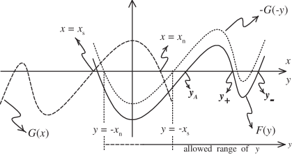
Figure 1: Shape of ${\cal G}(x)$ and ${\cal F}(y)$ for a general non-extremal charged massive dS C-metric studied in section III. The allowed range of $x$ is between $x_{\mathrm{s}}$ and $x_{\mathrm{n}}$ where ${\cal G}(x)$ is positive and compact. The permitted range of $y$ is $-x\leq y<+\infty$. The presence of an accelerated horizon is indicated by $y_{A}$ and the inner and outer charged horizons by $y_{-}$ and $y_{+}$. In the Nariai case, $y_{+}$ and $y_{A}$ coincide (see section III.2), in the Bertotti-Robinson case, $y_{-}$ and $y_{+}$ coincide (see section III.3), and in the Nariai Bertotti-Robinson case, $y_{-}$, $y_{+}$ and $y_{A}$ coincide (see section III.4). In the cases studied in this paper, ${\cal G}(x)$ has only two real zeros, $x_{\mathrm{s}}$ and $x_{\mathrm{n}}$.

The solution has a curvature singularity at $y=+\infty$, and $y$ must belong to the range $-x\leq y<+\infty$. The point $y=-x$ corresponds to a point that is infinitely far away from the curvature singularity, thus as $y$ increases we approach the curvature singularity and $y+x$ is the inverse of a radial coordinate. At most, ${\cal F}(y)$ can have four real zeros which we label in ascending order by $y_{\rm neg}<0<y_{A}\leq y_{+}\leq y_{-}$. The roots $y_{-}$ and $y_{+}$ are respectively the inner and outer charged black hole horizons, and $y_{A}$ is an acceleration horizon which coincides with the cosmological horizon and has a non-spherical shape, although the topology is spherical. The negative root $y_{\rm neg}$ satisfies $y_{\rm neg}<-x$ and has no physical significance, i.e., it does not belong to the range accessible to $y$.

We will demand that $x$ belongs to the interval $x_{\mathrm{s}}\leq x\leq x_{\mathrm{n}}$, sketched in Fig. 1 where ${\cal G}(x)\geq 0$. By doing this we guarantee that the metric has the correct signature $(-+++)$ [see Eq. (25)] and that the angular surfaces $t=$const and $y=$const are compact. For a reason that we shall explain soon we will label these surfaces by $\tilde{S}^{2}$. In these angular surfaces we now define two new coordinates,

$$\theta=\int_{x}^{x_{\mathrm{n}}}{\cal{G}}^{-1/2}dx\>,\hskip 28.45274pt\phi = z/\kappa\>,$$ (29)

where $\phi$ ranges between $[0,2\pi]$ and $\kappa$ is an arbitrary positive constant which will be discussed later. The coordinate $\theta$ ranges between the north pole, $\theta=\theta_{\mathrm{n}}=0$, and the south pole, $\theta=\theta_{\mathrm{s}}$ (not necessarily at $\pi$). Rewritten as a function of these new coordinates, the angular part of the metric becomes $ds_{\tilde{S}^{2}}^{2}=d\theta^{2}+\kappa^{2}{\cal G}\,d\phi^{2}$. Note that when we set $A=0$ we have $x_{\mathrm{s}}\leq x\leq x_{\mathrm{n}}$, with $x_{\mathrm{s}}=-1$ and $x_{\mathrm{n}}=1$, $x=\cos\theta$, ${\cal G}=1-x^{2}=\sin^{2}\theta$, and $\kappa=1$. Therefore, in this case the compact angular surface $\tilde{S}^{2}$ is a round $S^{2}$ sphere which justifies the label given to the new angular coordinates. When we set $A\neq 0$ the compact angular surface turns into a deformed 2-sphere that we represent onwards by $\tilde{S}^{2}$.

Recently, the issue of the gravitational radiation emitted by uniformly accelerated sources without horizons has been analyzed by Bičák and Krtouš BicKrt and the radiative properties of accelerated black holes in dS background have been analyzed by Krtouš and Podolský KrtPod .

III.2 The Nariai C-metric

We will generate the Nariai C-metric from a special extremal limit of the dS C-metric. First we will describe this particular near-extreme solution and then we will generate the Nariai C-metric.

We are interested in a particular extreme dS C-metric, for which the size of the acceleration horizon $y_{A}$ is equal to the size of the outer charged horizon $y_{+}$. Let us label this degenerated horizon by $\rho$, i.e., $y_{A}=y_{+}\equiv\rho$ with $\rho<y_{-}$. In this case, the function ${\cal F}(y)$ can be written as

$${\cal F}(y)=\frac{\rho^{2}-3\gamma}{\rho^{4}}(y-y_{\rm neg})(y-y_{-})(y-\rho)^{2}\>,$$ (30)

where

$$\gamma=\frac{\Lambda+3A^{2}}{3A^{2}}\>,$$ (31)

and the roots $\rho$, $y_{\rm neg}$ and $y_{-}$ are given by

$$\rho=\frac{3m}{4q^{2}A}\left(1-\sqrt{1-\frac{8}{9}\frac{q^{2}}{m^{2}}}\>\right)\>,$$ (32)

$$y_{\rm neg}=\frac{\gamma\rho}{\rho^{2}-3\gamma}\left(1-\sqrt{\frac{\rho^{2}-2\gamma}{\gamma}}\>\right)\>,$$ (33)

$$y_{-}=\frac{\gamma\rho}{\rho^{2}-3\gamma}\left(1+\sqrt{\frac{\rho^{2}-2\gamma}{\gamma}}\>\right)\>.$$ (34)

The mass and the charge of the solution are written as functions of $\rho$ as

$$m=\frac{1}{A\rho}\left(1-\frac{2\gamma}{\rho^{2}}\right)\>,$$

$$q^{2}=\frac{1}{A^{2}\rho^{2}}\left(1-\frac{3\gamma}{\rho^{2}}\right)\>.$$ (35)

The conditions $\rho<y_{-}$ and $q^{2}\geq 0$ require that the allowed range of $\rho$ is

$$\sqrt{3\gamma}\leq\rho<\sqrt{6\gamma}\>.$$ (36)

The value of $y_{-}$ decreases monotonically with $\rho$ and we have $\sqrt{6\gamma}<y_{-}<+\infty$. The mass and the charge of the Nariai solution, denoted now as $m_{\rm N}$ and $q_{\rm N}$ respectively, are monotonically increasing functions of $\rho$, and as we go from $\rho=\sqrt{3\gamma}$ into $\rho=\sqrt{6\gamma}$ we have

$$\frac{1}{3}\frac{1}{\sqrt{\Lambda+3A^{2}}}\leq m_{\rm N}<\frac{\sqrt{2}}{3}\frac{1}{\sqrt{\Lambda+3A^{2}}}\>,$$

$$0\leq q_{\rm N}<\frac{1}{2}\frac{1}{\sqrt{\Lambda+3A^{2}}}\>,$$ (37)

so the $A\neq 0$ extreme ($y_{A}=y_{+}$) solution has a lower maximum mass and charge, and has a lower minimum mass than the corresponding $A=0$ solution MelMosRom ; MannRoss ; BooMann , and, for a fixed $\Lambda$, as the acceleration parameter $A$ grows these extreme values decrease monotonically. For a fixed $\Lambda$ and for a fixed mass between $\sqrt{1/(9\Lambda)}\leq m<\sqrt{2/(9\Lambda)}$, the allowed acceleration varies as $\sqrt{1/(27m^{2})-\Lambda/3}\leq A<\sqrt{2/(27m^{2})-\Lambda/3}$.

We are now ready to obtain the Nariai C-metric. In order to generate it from the above near-extreme dS C-metric we first set

$$y_{A}=\rho-\varepsilon,\>\>\>\>y_{+}=\rho+\varepsilon,\>\>\>\>\>\>{\rm with}\>\>\varepsilon<<1\>,$$ (38)

in order that $\varepsilon$ measures the deviation from degeneracy, and the limit $y_{A}\rightarrow y_{+}$ is obtained when $\varepsilon\rightarrow 0$. Now, we introduce a new time coordinate $\tau$ and a new radial coordinate $\chi$,

$$t=\frac{1}{\varepsilon{\cal K}}\,\tau\>,\>\>\>\>\>\>\>\>\>\>\>y=\rho+\varepsilon\cos\chi\>,$$ (39)

where

$${\cal K}=-\frac{\rho^{2}-3\gamma}{\rho^{4}}(\rho-y_{\rm neg})(\rho-y_{-})=\frac{2(\Lambda+3A^{2})}{A^{2}\rho^{2}}-1\>,$$

(40)

and condition (36) implies $0<{\cal K}\leq 1$ with $q=0\Rightarrow{\cal K}=1$. In the limit $\varepsilon\rightarrow 0$, from (25) and (30), we get the gravitational field of the Nariai C-metric

$$ds^{2} = \frac{{\cal R}^{2}(x)}{{\cal K}}\left(-\sin^{2}\chi\,d\tau^{2}+d\chi^{2}\right)$$ (41)

$$+{\cal R}^{2}(x)\left[{\cal G}^{-1}(x)dx^{2}+{\cal G}(x)dz^{2}\right]\>,$$

where $\chi$ runs from $0$ to $\pi$ and

$${\cal R}^{2}(x)=\left(Ax+\sqrt{\frac{2(\Lambda+3A^{2})}{1+{\cal K}}}\right)^{-2}\>,$$

$$\!\!\!\!\!\!\!\!\!{\cal G}(x)=1-x^{2}-\frac{2A}{3}\sqrt{\frac{(1+{\cal K})(2-{\cal K})^{2}}{2(\Lambda+3A^{2})}}\,x^{3}-\frac{A^{2}}{4}\frac{1-{\cal K}^{2}}{\Lambda+3A^{2}}\,x^{4}\,.$$

(42)

${\cal G}(x)$ has only two real roots, the south pole $x_{\mathrm{s}}$ and the north pole $x_{\mathrm{n}}$. The angular coordinate $x$ can range between these two poles, whose values are calculated in Appendix B. Under the coordinate transformation (39), the Maxwell field for the magnetic case is still given by Eq. (27), while in the electric case, (28) becomes

$$F=\frac{q}{{\cal K}}\,\sin\chi\,d\tau\wedge d\chi\>.$$ (43)

So, if we give the parameters $\Lambda$, $A$, and $q$ we can construct the Nariai C-metric. The Nariai C-metric is conformal to the topological product of two 2-dimensional manifolds, $dS_{2}\times\tilde{S}^{2}$, with the conformal factor ${\cal R}^{2}(x)$ depending on the angular coordinate $x$, and $\tilde{S}^{2}$ being a deformed 2-sphere.

In order to obtain the $A=0$ limit, we first set $\tilde{\rho}=A\rho$ [see Eq. (32)], a parameter that has a finite and well-defined value when $A\rightarrow 0$. Then when $A\rightarrow 0$ we have ${\cal K}\rightarrow{\cal K}_{0}=2\Lambda/\tilde{\rho}^{2}-1$ and ${\cal R}^{2}(x)\rightarrow{\cal R}_{0}^{\>2}=\tilde{\rho}^{-2}$, with ${\cal R}_{0}^{\>2}$ and ${\cal K}_{0}$ satisfying relations (5). This, together with transformations (29), show that the Nariai C-metric transforms into the Nariai solution (2) when $A=0$.

The limiting procedure that has been applied in this subsection has generated a new exact solution that satisfies the Maxwell-Einstein equations in a positive cosmological constant background.

In order to give a physical interpretation to this extremal limit of the dS C-metric, we first recall the physical interpretation of the dS C-metric. This solution describes a pair of uniformly accelerated black holes in a dS background, with the acceleration being provided by the cosmological constant and by a strut between the black holes that pushes them away or, alternatively, by a string that connects and pulls the black holes in. The presence of the strut or of the string is associated to the conical singularities that exist in the C-metric (see, e. g., OscLem_dS-C ). Indeed, in general, if we draw a small circle around the north or south pole, as the radius goes to zero, the limit circunference/radius is not $2\pi$. There is a deficit angle at the north pole given by (see OscLem_AdS-C ; OscLem_dS-C ), $\delta_{\mathrm{{n}}}=2\pi\left(1-\frac{\kappa}{2}|{\cal G}^{\prime}(x_{\mathrm{n}})|\right)$ (where the prime means derivative with respect to $x$) and, analogously, a similar conical singularity ($\delta_{\mathrm{{s}}}$) is present at the south pole. The so far arbitrary parameter $\kappa$ introduced in Eq. (29) plays its important role here. Indeed, if we choose $\kappa^{-1}=\frac{1}{2}|{\cal G}^{\prime}(x_{\mathrm{s}})|$ we remove the conical singularity at the south pole ($\delta_{\mathrm{s}}=0$). However, since we only have a single constant $\kappa$ at our disposal and this has been fixed to avoid the conical singularity at the south pole ($\delta_{\mathrm{s}}=0$), we conclude that a conical singularity will be present at the north pole with $\delta_{\mathrm{n}}<0$. This is associated to a strut (since $\delta_{\mathrm{n}}<0$) that joins the two black holes along their north poles and provides their acceleration. This strut satisfies the relation $p=-\mu>0$, where $p$ and $\mu=\delta_{\mathrm{n}}/(8\pi)$ are respectively its pressure and its mass density (see OscLem_AdS-C ). There is another alternative. We can choose instead $\kappa^{-1}=\frac{1}{2}|{\cal G}^{\prime}(x_{\mathrm{n}})|$ and by doing so we avoid the deficit angle at the north pole ($\delta_{\mathrm{n}}=0$), and leave a conical singularity at the south pole ($\delta_{\mathrm{s}}>0$). This option leads to the presence of a string (with $p=-\mu<0$) connecting the black holes along their south poles that furnishes the acceleration. Summarizing, when the conical singularity is at the north pole, the pressure of the strut is positive, so it points outwards and pushes the black holes apart, furnishing their acceleration. When the conical singularity is at the south pole, it is associated to a string between the two black holes with negative pressure that pulls the black holes away from each other.

The causal structure of the dS C-metric has been analyzed in detail in OscLem_dS-C . The Carter-Penrose diagram of the non-extreme charged dS C-metric is sketched in Fig. 2.(a) (whole figure) and has a structure that, loosely speaking, can be divided into left, middle and right regions. The middle region contains the null infinity, the past infinity, ${\cal I^{-}}$, and the future infinity, ${\cal I^{+}}$, and an accelerated Rindler-like horizon, $h_{A}$ (that coincides with the cosmological horizon). The left and right regions both contain a timelike curvature singularity (the zig-zag line), and an inner ($h_{-}$) and an outer ($h_{+}$) horizons associated to the charged character of the solution. This diagram represents two dS$-$Reissner-Nordström black holes that approach asymptotically the Rindler-like acceleration horizon (for a more detailed discussion see OscLem_dS-C ). This is also schematically represented in Fig. 3 (whole figure), where we explicitly show the strut that connects the two black holes and provides their acceleration.

Now, as we have just seen, the Nariai C-metric can be appropriately obtained from the vicinity of the black hole and acceleration horizons in the limit in which the size of these two horizons approach each other. We now will see that the conical singularity of the dS C-metric survives the near-extremal limiting procedure that generates the Nariai C-metric. Following an elucidative illustration shown in MaldStrom for the Bertotti-Robinson solution (with $\Lambda<0$ and $A=0$), this near-horizon region is sketched in Fig. 2.(a) as a shaded area, and from it we can identify some of the features of the Nariai C-metric, e.g., the curvature singularity of the original dS black hole is lost in the near-extremal limiting procedure. But, more important, this shaded near-horizon region also allows us to construct straightforwardly the Carter-Penrose diagram of the Nariai C-metric drawn in Fig. 2.(b). The construction steps are as follows. First, as indicated by (38) and the second relation of (39), we let the cross lines that represent the black hole horizon [$h_{+}$ in Fig. 2.(a)] join together with the cross lines that represent the acceleration horizon [$h_{A}$ in Fig. 2.(a)], and so on, i.e., we do this joining ad infinitum with all the cross lines $h_{+}$ and $h_{A}$. After this step all that is left from the original diagram is a single cross line, i.e, all the spacetime that has originally contained in the shaded area of Fig. 2.(a) has collapsed into two mutually perpendicular lines at $45^{\circ}$ at $y=\rho$. Now, as indicated by the first relation of (39), when $\varepsilon\rightarrow 0$ the time suffers an infinite blow up. To this blow up in the time corresponds an infinite expansion in the Carter-Penrose diagram in the vicinity of $y=\rho$. We then get again the shaded area of Fig. 2.(a), but now the cross lines of this shaded area are all identified into a single horizon, and they no longer have the original signature associated to $h_{+}$ and $h_{A}$ that differentiated them. This is, in the shaded area of Fig. 2.(a) we must now erase the original labels $h_{+}$ and $h_{A}$. The Carter-Penrose diagram of the Nariai C-metric is then given by Fig. 2.(b), which is equivalent to the diagram of the (1+1)-dimensional dS solution. Note that the diagram of the $A=0$ dS$-$Reissner-Nordström solution is identical to the one of Fig. 2.(a), as long as we replace $h_{A}$ (acceleration horizon) by $h_{c}$ (cosmological horizon). Applying the same construction process described just above we find that the Carter-Penrose diagram of the Nariai solution ($A=0$), described in subsection II.1, is also given by Fig. 2.(b).

Figure 2: (a) The whole figure is the Carter-Penrose diagram of the dS C-metric. The shaded region represents the near-horizon area that, when the black hole horizon ($h_{+}$) approaches the acceleration horizon ($h_{+}$), gives the $dS_{2}$ manifold of the Nariai C-metric solution. See discussion in the text. (b) Carter-Penrose diagram of the Nariai C-metric.

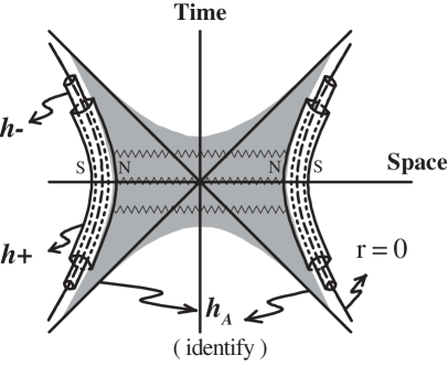
Figure 3: The whole figure represents schematically the two black holes of the dS C-metric approaching asymptotically the Rindler-like acceleration horizon. They are accelerated by a strut that joins them along their north poles. The shaded region represents the near-horizon area that, when the black hole horizon approaches the acceleration horizon, gives the Nariai C-metric solution (compare with Fig. 2). The strut survives to the limiting process.

The Nariai near-horizon region is also sketched in Fig. 3 as a shaded area. This schematic figure is clarifying in the sense that it indicates that the strut that connects the two original black holes along their north pole directions survives to the near-extremal limiting process and will be present in the final result of the process, i.e., in the Nariai C-metric. Indeed, note that the endpoints of the strut are at the north pole of the event horizons of the two black holes and crosses the acceleration horizon. As we saw just above, this region suffers first a collapse followed by an infinite blow up and during the process the strut is not lost. Thus the Nariai C-metric (41)-(42) describes a spacetime that is conformal to the product $dS_{2}\times\tilde{S}^{2}$. To each point in the deformed 2-sphere corresponds a $dS_{2}$ spacetime, except for one point which corresponds a $dS_{2}$ spacetime with an infinite straight strut. This strut has negative mass density given by

$$\mu=\frac{1}{4}{\biggl{(}}1-{\biggl{|}}\frac{{\cal G}^{\prime}(x_{\mathrm{{n}}})}{{\cal G}^{\prime}(x_{\mathrm{{s}}})}{\biggl{|}}{\biggr{)}}\>,$$ (44)

where ${\cal G}^{\prime}(x)$ is the derivative of Eq. (42), and with a positive pressure $p=-\mu>0$. Alternatively, if we remove the conical singularity at the north pole, the Nariai C-metric describes a string with positive mass density $\mu=(1/4)\left(1-|{\cal G}^{\prime}(x_{\mathrm{{s}}})/{\cal G}^{\prime}(x_{\mathrm{{n}}})|\right)$ and negative pressure $p=-\mu<0$.

As we have said in subsection II.1, the Nariai solution ($A=0$) is unstable and, once created, it decays through the quantum tunnelling process into a slightly non-extreme black hole pair. We then expect that the Nariai C-metric is also unstable and that it will decay into a slightly non-extreme pair of black holes accelerated by a strut or by a string. The Nariai C-metric instanton also plays an important role in the decay of the dS space, since it can mediate the Schwinger-like quantum process of pair creation of black holes in a dS background OscLem-PCdS . Indeed, as we said in subsection II.1, the Nariai instanton ($A=0$) has been used MelMosRom ; MannRoss ; BooMann ; VolkovWipf to study the pair creation of dS black holes materialized and accelerated by the cosmological background field. Moreover, the Euclidean “Nariai” flat C-metric flatPC and Ernst solution ErnstPC (also discussed in this paper in section III.1) have been used to analyze the process of pair production of $\Lambda=0$ black holes, accelerated by a string or by an electromagnetic external field, respectively. Therefore, it is natural to expect that the Euclidean Nariai limit of the dS C-metric mediates the process of pair creation of black holes in a cosmological background, that are then accelerated by a string, in addition to the cosmological background field. The picture would be that of the nucleation, in a dS background, of a Nariai C universe, whose string then breaks down and a pair of dS black holes is created at the endpoints of the string. This expectation is confirmed in OscLem-PCdS .

III.3 The Bertotti-Robinson dS C-metric

Now, we are interested in another particular extreme dS C-metric (usually called cold solution when $A=0$ MelMosRom ; MannRoss ; BooMann ) for which the size of the outer charged black hole horizon $y_{+}$ is equal to the size of the inner charged horizon $y_{-}$. Let us label this degenerated horizon by $\rho$, such that, $y_{+}=y_{-}\equiv\rho$ and $\rho>y_{A}$. This solution requires the presence of the electromagnetic charge. In this case, the function ${\cal F}(y)$ can be written as

$${\cal F}(y)=\frac{\rho^{2}-3\gamma}{\rho^{4}}(y-y_{\rm neg})(y-y_{A})(y-\rho)^{2}\>,$$ (45)

with $\gamma$ given by Eq. (31), the roots $\rho$ and $y_{\rm neg}$ are defined by Eqs. (32) and (33), respectively, and $y_{A}$ is given by

$$y_{A}=\frac{\gamma\rho}{\rho^{2}-3\gamma}\left(1+\sqrt{\frac{\rho^{2}-2\gamma}{\gamma}}\>\right)\>.$$ (46)

Eq. (35) defines the mass and the charge of the solution as a function of $\rho$, and, for a fixed $A$ and $\Lambda$, the ratio $q/m$ is higher than $1$. The conditions $\rho>y_{A}$ and $q^{2}>0$ require that the allowed range of $\rho$ is

$$\rho>\sqrt{6\gamma}\>.$$ (47)

The value of $y_{A}$ decreases monotonically with $\rho$ and we have $\sqrt{\gamma}<y_{A}<\sqrt{6\gamma}$. Contrary to the Nariai case, the mass and the charge of the Bertotti-Robinson solution, $m_{\rm BR}$ and $q_{\rm BR}$, respectively, are monotonically decreasing functions of $\rho$, and as we come from $\rho=+\infty$ into $\rho=\sqrt{6\gamma}$ we have

$$0<m_{\rm BR}<\frac{\sqrt{2}}{3}\frac{1}{\sqrt{\Lambda+3A^{2}}}\>,$$

$$0<q_{\rm BR}<\frac{1}{2}\frac{1}{\sqrt{\Lambda+3A^{2}}}\>,$$ (48)

so the $A\neq 0$ extreme ($y_{+}=y_{-}$) solution has a lower maximum mass and charge than the corresponding $A=0$ solution MelMosRom ; MannRoss ; BooMann and, for a fixed $\Lambda$, as the acceleration parameter $A$ grows this maximum value decreases monotonically. For a fixed $\Lambda$ and for a fixed mass below $\sqrt{2/(9\Lambda)}$, the maximum value of the acceleration is $\sqrt{2/(27m^{2})-\Lambda/3}$.

We are now ready to generate the Bertotti-Robinson dS C-metric from the above cold dS C-metric. We first set

$$y_{+}=\rho-\varepsilon,\>\>\>\>y_{-}=\rho+\varepsilon,\>\>\>\>\>\>{\rm with}\>\>\varepsilon<<1\>,$$ (49)

in order that $\varepsilon$ measures the deviation from degeneracy, and the limit $y_{+}\rightarrow y_{-}$ is obtained when $\varepsilon\rightarrow 0$. Now, we introduce a new time coordinate $\tau$ and a new radial coordinate $\chi$,

$$t=\frac{1}{\varepsilon{\cal K}}\,\tau\>,\>\>\>\>\>\>\>\>\>\>\>y=\rho+\varepsilon\cosh\chi\>,$$ (50)

where

$${\cal K}=\frac{\rho^{2}-3\gamma}{\rho^{4}}(\rho-y_{\rm neg})(\rho-y_{A})=1-\frac{2(\Lambda+3A^{2})}{A^{2}\rho^{2}}\>,$$

(51)

and condition (47) implies $0<{\cal K}<1$. In the limit $\varepsilon\rightarrow 0$, from (25) and (45), the metric becomes

$$ds^{2} = \frac{{\cal R}^{2}(x)}{{\cal K}}\left(-\sinh^{2}\chi\,d\tau^{2}+d\chi^{2}\right)$$ (52)

$$+ {\cal R}^{2}(x)\left[{\cal G}^{-1}(x)dx^{2}+{\cal G}(x)dz^{2}\right]\>,$$

where $\chi$ is unbounded and

$${\cal R}^{2}(x)=\left(Ax+\sqrt{\frac{2(\Lambda+3A^{2})}{1-{\cal K}}}\right)^{-2}\>,$$

$${\cal G}(x)=1-x^{2}-\frac{2A}{3}\sqrt{\frac{(1-{\cal K})(2+{\cal K})^{2}}{2(\Lambda+3A^{2})}}\,x^{3}-\frac{A^{2}}{4}\frac{1-{\cal K}^{2}}{\Lambda+3A^{2}}\,x^{4}\>.$$

(53)

${\cal G}(x)$ has only two real roots, the south pole $x_{\mathrm{s}}$ and the north pole $x_{\mathrm{n}}$. The angular coordinate $x$ can range between these two poles whose value is calculated in appendix B. Under the coordinate transformation (50), the Maxwell field for the magnetic case is still given by Eq. (27), while in the electric case, (28) becomes

$$F=-\frac{q}{{\cal K}}\,\sinh\chi\,d\tau\wedge d\chi\>.$$ (54)

So, if we give the parameters $\Lambda$, $A$, and $q$ we can construct the Bertotti-Robinson dS C-metric. This solution is conformal to the topological product of two 2-dimensional manifolds, $AdS_{2}\times\tilde{S}^{2}$, with the conformal factor ${\cal R}^{2}(x)$ depending on the angular coordinate $x$.

In order to obtain the $A=0$ limit, we first set $\tilde{\rho}=A\rho$ [see Eq. (32)], a parameter that has a finite and well-defined value when $A\rightarrow 0$. Then when $A\rightarrow 0$ we have ${\cal K}\rightarrow{\cal K}_{0}=1-2\Lambda/\tilde{\rho}^{2}$ and ${\cal R}^{2}(x)\rightarrow{\cal R}_{0}^{\>2}=\tilde{\rho}^{-2}$. This, together with transformations (29), show that the Bertotti-Robinson dS C-metric transforms into the dS counterpart of the Bertotti-Robinson solution discussed in subsection II.2, when $A=0$. The limiting procedure that has been applied in this subsection has generated a new exact solution that satisfies the Maxwell-Einstein equations in a positive cosmological constant background.

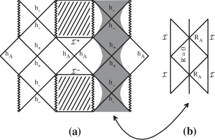
Figure 4: (a) The whole figure is the Carter-Penrose diagram of the dS C-metric. The shaded region represents the near-horizon area that, when the inner black hole horizon ($h_{-}$) approaches the outer black hole horizon ($h_{+}$), gives the $AdS_{2}$ manifold of the Bertotti-Robinson C-metric. See discussion in the text. (b) Carter-Penrose diagram of the Bertotti-Robinson C-metric.

We have just seen that the Bertotti-Robinson dS C-metric can be appropriately obtained from the vicinity of the inner and outer black hole horizons in the limit in which the size of these two horizons approach each other. This near-horizon region is sketched in Fig. 4.(a) as a shaded area, and from it we can construct straightforwardly the Carter-Penrose diagram of the Bertotti-Robinson dS C-metric drawn in Fig. 4.(b). The construction steps are as follows. First, as indicated by (49) and the second relation of (50), we let the cross lines that represent the black hole Cauchy horizon [$h_{-}$ in Fig. 4.(a)] join together with the cross lines that represent the black hole event horizon [$h_{+}$ in Fig. 4.(a)], and so on, i.e., we do this junction ad infinitum with all the cross lines $h_{-}$ and $h_{+}$. After this step all that is left from the original diagram is a single cross line, i.e, all the spacetime that has originally contained in the shaded area of Fig. 4.(a) has collapsed into two mutually perpendicular lines at $45^{\circ}$ at $y=\rho$. Now, as indicated by the first relation of (50), when $\varepsilon\rightarrow 0$ the time suffers an infinite blow up. To this blow up in the time corresponds an infinite expansion in the Carter-Penrose diagram in the vicinity of $y=\rho$ that generates an $AdS_{2}$ region. We then get again the shaded area of Fig. 4.(a), but now the cross lines of this shaded area are all identified into a single line, and they no longer have the original lables associated to $h_{-}$ and $h_{+}$ that differentiated them. This is, in the shaded area of Fig. 4.(a) we must now erase the original labels $h_{-}$ and $h_{+}$. The Carter-Penrose diagram of the Bertotti-Robinson dS C-metric is then given by Fig. 4.(b), which is equivalent to the diagram of the (1+1)-dimensional AdS solution. Note that the diagram of the $A=0$ Reissner-Nordström$-$dS solution is identical to the one of Fig. 4.(a). Therefore, applying the same construction process described just above we find that the Carter-Penrose diagram of the Bertotti-Robinson dS solution ($A=0$) is similar to the one of Fig. 4.(b). The diagram of the Bertotti-Robinson solution with $\Lambda=0$ described by (10) is also given by Fig. 4.(b).

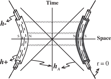
Figure 5: The whole figure represents schematically the two accelerated black holes of the dS C-metric. The shaded region represents the near-horizon area that, when the inner black hole horizon approaches the outer black hole horizon, gives the Bertotti-Robinson C-metric (compare with Fig. 4). The strut does not survive to the limiting process.

The Bertotti-Robinson near-horizon region is also sketched in Fig. 5 as a shaded area. This schematic figure is clarifying in the sense that it indicates that the strut that connects the two original black holes along their north pole directions does not survive to the near-extremal limiting process and will not be present in the final result of the process, i.e., in the Bertotti-Robinson dS C-metric. However, a reminiscence of this strut remains in the final solution. Indeed, the angular factor of the Bertotti-Robinson dS C-metric [which, remind, describes a deformed 2-sphere $\tilde{S}^{2}$ with a fixed size ${\cal R}^{2}(x)$ given by (53)] has a conical singularity at least at one of its poles. We can choose the parameter $\kappa$, introduced in (29), in order to have a conical singularity only at the north pole ($\delta_{\mathrm{s}}=0$), or only at the south pole ($\delta_{\mathrm{n}}=0$), however we cannot eliminate both. When the parameter $A$ is set to zero, the conical singularities disappear, the angular factor describes a round 2-sphere with fixed radius, and the Bertotti-Robinson dS C-metric reduces into the Bertotti-Robinson dS solution with topology $AdS_{2}\times S^{2}$.

III.4 The Nariai Bertotti-Robinson dS C-metric

As the previous sections and the label suggest, the Nariai Bertotti-Robinson dS C-metric will be generated from the extremal limit of a very particular dS C-metric (usually called ultracold solution when $A=0$ MelMosRom ; MannRoss ; BooMann ) for which the size of the three horizons ($y_{A}$, $y_{+}$ and $y_{-}$) are equal, and let us label this degenerated horizon by $\rho$: $y_{A}=y_{+}=y_{-}\equiv\rho$. In this case, the function ${\cal F}(y)$ is given by Eq. (30) with $y_{-}=\rho$, and $\gamma$ defined in Eq. (31). The negative root $y_{\rm neg}$ is given by Eq. (33) and

$$\rho=\sqrt{6\gamma}\>.$$ (55)

The mass and the charge of the Nariai Bertotti-Robinson dS C-metric solution , $m_{\rm NBR}$ and $q_{\rm NBR}$, respectively, are given by

$$m_{\rm NBR}=\frac{\sqrt{2}}{3}\sqrt{\frac{1}{\Lambda+3A^{2}}}\>,$$

$$q_{\rm NBR}=\frac{1}{2}\sqrt{\frac{1}{\Lambda+3A^{2}}}\>,$$ (56)

and these values are the maximum values of the mass and charge of both the Nariai C and Bertotti-Robinson C solutions, Eqs. (37) and (48), respectively. To clarify the nature of these solutions, a diagram $m\sqrt{\Lambda+3A^{2}}\times q\sqrt{\Lambda+3A^{2}}$ is plotted in Fig. 6. For a fixed value of $A$ and $\Lambda$, the allowed range of the mass and charge of the Nariai C-metric, of the Bertotti-Robinson dS C-metric, and of the Nariai Bertotti-Robinson dS C-metric is shown.

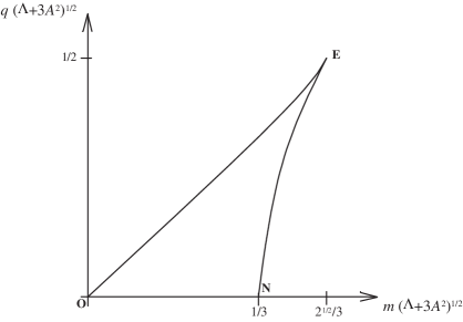
Figure 6: Relation $m\sqrt{\Lambda+3A^{2}}\times q\sqrt{\Lambda+3A^{2}}$, for a fixed value of $A$ and $\Lambda$, for the extremal limits of the dS C-metric. $NE$ represents the Nariai C-metric (with point $N$ representing the neutral case), $OE$ represents the Bertotti-Robinson dS C-metric, and point $E$ represents the Nariai Bertotti-Robinson dS C-metric.

We are now ready to generate the Nariai Bertotti-Robinson dS C-metric from the above ultracold dS C-metric. We first set

$$\rho=\sqrt{6\gamma}-\varepsilon,\>\>\>\>y_{-}=\sqrt{6\gamma}+\varepsilon\>,\>\>\>\>\>\>{\rm with}\>\>\varepsilon<<1\>.$$ (57)

Now, we introduce a new time coordinate $\tau$ and a new radial coordinate $\chi$,

$$t=\frac{1}{2\varepsilon^{2}{\cal K}}\,\tau\>,\>\>\>\>\>\>\>\>\>\>\>y=\sqrt{6\gamma}+\varepsilon\cosh(\sqrt{2\varepsilon{\cal K}}\>\chi)\>,$$ (58)

where

$${\cal K} = \frac{\rho^{2}-3\gamma}{\rho^{4}}(\rho-y_{\rm neg})=\frac{1}{3}\sqrt{\frac{2A^{2}}{\Lambda+3A^{2}}}\>.$$ (59)

In the limit $\varepsilon\rightarrow 0$ the metric (25) becomes

$$ds^{2}\!\! = \!\!{\cal R}^{2}(x)\left[-\chi^{2}\,d\tau^{2}+d\chi^{2}+{\cal G}^{-1}(x)dx^{2}+{\cal G}(x)dz^{2}\right],$$

with

$${\cal R}^{2}(x)=\left(Ax+\sqrt{2(\Lambda+3A^{2})}\right)^{-2}\>,$$

$${\cal G}(x)=1-x^{2}-\frac{2A}{3}\sqrt{\frac{2}{\Lambda+3A^{2}}}\,x^{3}-\frac{A^{2}}{4(\Lambda+3A^{2})}\,x^{4}\>.$$ (61)

${\cal G}(x)$ has only two real roots, the south pole $x_{\mathrm{s}}$ and the north pole $x_{\mathrm{n}}$. The angular coordinate $x$ can range between these two poles whose value is calculated in appendix B. Notice that the spacetime factor $-\chi^{2}\,d\tau^{2}+d\chi^{2}$ is just ${\mathbb{M}}^{1,1}$ in Rindler coordinates. Therefore, under the usual coordinate transformation $\chi=\sqrt{\bar{x}^{2}-\bar{t}^{\,2}}$ and $\tau={\rm arctanh(\bar{t}/\bar{x})}$, this factor transforms into $-d\bar{t}^{\,2}+d\bar{x}^{2}$. Under the coordinate transformation (58), the Maxwell field for the magnetic case is still given by Eq. (27), while in the electric case, (28) becomes

$$F=-q\,\chi\,d\tau\wedge d\chi\>.$$ (62)

The Nariai Bertotti-Robinson dS C-metric is conformal to the topological product of two 2-dimensional manifolds, ${\mathbb{M}}^{1,1}\times\tilde{S}^{2}$, with the conformal factor ${\cal R}^{2}(x)$ depending on the angular coordinate $x$.

In the $A=0$ limit, ${\cal R}^{2}(x)\rightarrow(2\Lambda)^{-1}$, and one obtains the Nariai Bertotti-Robinson solution $ds^{2}=(2\Lambda)^{-1}(-d\bar{t}^{\,2}+d\bar{x}^{2}+d\theta^{2}+\sin^{2}\theta\,d\phi^{2})$, which has the topology ${\mathbb{M}}^{1,1}\times S^{2}$ MelMosRom ; MannRoss ; BooMann ).

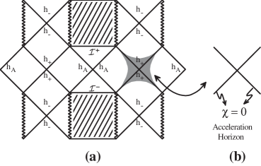
Figure 7: (a) The whole figure is the Carter-Penrose diagram of the dS C-metric. The shaded region represents the near-horizon area that, when the inner black hole horizon ($h_{-}$) and the acceleration horizon ($h_{A}$) approach the outer black hole horizon ($h_{+}$), gives the Rindler manifold of the Nariai Bertotti-Robinson C-metric. This shaded region is the intersection of the shaded areas of Figs. 2.(a) and 4.(a). See discussion in the text. (b) Kruskal diagram of the Nariai Bertotti-Robinson dS C-metric.

We have just seen that the Nariai Bertotti-Robinson dS C-metric can be appropriately obtained from the vicinity of the accelerated and black hole horizons in the limit in which the size of these three horizons approach each other. This near-horizon region is sketched in Fig. 7.(a) as a shaded area, and can be viewed as the intersection of the shaded areas of Figs. 2.(a) and 4.(a). From it we can construct straightforwardly, following the construction steps already sketched in subsections III.2 and III.3, the Kruskal diagram of the Nariai Bertotti-Robinson dS C-metric drawn in Fig. 7.(b). This diagram is equivalent to the Kruskal diagram of the Rindler solution. The strut that connects the two original black holes along their north pole directions survives to the near-extremal limiting process. Thus the Nariai Bertotti-Robinson dS C-metric describes a spacetime that is conformal to the product ${\mathbb{M}}^{1,1}\times\tilde{S}^{2}$. To each point in the deformed 2-sphere corresponds a ${\mathbb{M}}^{1,1}$ spacetime, except for one point which corresponds a ${\mathbb{M}}^{1,1}$ spacetime with an infinite straight strut or string, with a mass density and pressure satisfying $p=-\mu$. In an analogous way to the one that occurs with the Nariai C universe (see section IV.2), we expect that the Nariai Bertotti-Robinson dS C universe is unstable and, once created, it decays through the quantum tunnelling process into a slightly non-extreme black hole pair. The picture would be that of the nucleation, in a dS background, of a Nariai Bertotti-Robinson dS C universe, whose string then breaks down and a pair of dS black holes is created at the endpoints of the string. This expectation is confirmed in OscLem-PCdS . When the parameter $A$ is set to zero, the conical singularities disappear (and so the strut or string are no longer present) and the angular factor describes a round 2-sphere with fixed radius, and the topology of the Nariai Bertotti-Robinson dS C-metric reduces into ${\mathbb{M}}^{1,1}\times S^{2}$.

IV Extremal limits of the flat C-metric and of the Ernst solution

The Euclidean version of the “Nariai” flat C-metric that will be discussed in subsection IV.2 has already been used previously flatPC ; ErnstPC ; DGKT in the study of the quantum process of pair creation of black holes. However, as far as we know, the Bertotti-Robinson flat C-metric (discussed in subsection IV.3) and the Nariai Bertotti-Robinson flat C-metric (discussed in subsection IV.4) have not been written explicitly.

IV.1 The flat C-metric and the Ernst solution

IV.1.1 The flat C-metric

The gravitational field and the electromagnetic field of the massive charged flat C-metric is given by Eqs. (25)-(28) (see KW ), as long as we set $\Lambda=0$ in Eq. (26), and therefore we have now ${\cal F}(y)=-{\cal G}(-y)$ [see Fig. 8 for the general shape of ${\cal F}(y)$ and ${\cal G}(x)$]. The discussion of subsection III.1 applies then directly also to the $\Lambda=0$ case. In particular, in general the flat C-metric has a conical singularity at one of its poles that is interpreted KW as a strut joining the north poles of the two black holes that accelerates them apart, or alternatively, as two strings from infinity into the south pole of each one of the black holes that that pushes them into infinity. For the actual issue of the gravitational radiative properties of accelerated black holes described by the flat C-metric see Bičák, and Pravda and Pravdova BPP .

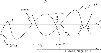
Figure 8: Shape of ${\cal G}(x)$ and ${\cal F}(y)$ for a general non-extremal charged massive flat C-metric studied in section IV. The allowed range of $x$ is between $x_{\mathrm{s}}$ and $x_{\mathrm{n}}$ where ${\cal G}(x)$ is positive and compact. The permitted range of $y$ is $-x\leq y<+\infty$. The presence of an accelerated horizon is indicated by $y_{A}$ and the inner and outer charged horizons by $y_{-}$ and $y_{+}$. In the “Nariai” case, $y_{+}$ and $y_{A}$ coincide (see section IV.2), in the Bertotti-Robinson case, $y_{-}$ and $y_{+}$ coincide (see section IV.3), and in the Nariai Bertotti-Robinson case, $y_{-}$, $y_{+}$ and $y_{A}$ coincide (see section IV.4). Note that when $y_{+}$ and $y_{A}$ coincide, the same occurs with $x_{\mathrm{s}}$ and $x_{0}$.

IV.1.2 The Ernst solution

Ernst Ernst has employed a Harrison-type transformation to the charged flat C-metric in order to append a suitably chosen external electromagnetic field. With this procedure the Ernst solution is free of conical singularities at both poles and the acceleration that drives away the two oppositely charged Reissner-Nordström black holes is provided by the external electromagnetic field. The gravitational field of the Ernst solution is Ernst

$$ds^{2}=\frac{\Sigma^{2}(-{\cal F}dt^{2}+{\cal F}^{-1}dy^{2}+{\cal G}^{-1}dx^{2}+\Sigma^{-4}{\cal G}\,dz^{2})}{[A(x+y)]^{2}}\>,$$

(63)

where ${\cal F}(y)$ and ${\cal G}(x)$ are given by (26) with $\Lambda=0$, and

$$\Sigma(x,y)={\biggl{(}}1+\frac{1}{2}\,q\,{\cal E}_{0}\,x{\biggr{)}}^{2}+\frac{{\cal E}_{0}^{2}\,{\cal G}(x)}{4A^{2}\,(x+y)^{2}}\>.$$ (64)

In the electric solution one has $q\equiv e$ and ${\cal E}_{0}\equiv E_{0}$, i.e., $q$ and ${\cal E}_{0}$ are respectively the electric charge and the external electric field. In the magnetic solution one has $q\equiv g$ and ${\cal E}_{0}\equiv B_{0}$, i.e., $q$ and ${\cal E}_{0}$ are respectively the magnetic charge and the external magnetic field. The electromagnetic potential of the magnetic Ernst solution is Ernst

$$A_{z}=-\frac{2}{\Sigma\,B_{0}}{\biggl{(}}1+\frac{1}{2}\,g\,B_{0}\,x{\biggr{)}}\>.$$ (65)

while for the electric Ernst solution it is given by Brown

$$A_{t} = qy-\frac{E_{0}}{2A^{2}}\frac{{\cal F}(y)}{(x+y)^{2}}\left(1+e\,E_{0}\,x-\frac{1}{2}e\,E_{0}\,y\right)$$

$$- \frac{E_{0}}{2A^{2}}(1+r_{-}Ay)(1+r_{+}Ay)(1-e\,E_{0}\,y/2)\>,$$

with $r_{+}r_{-}=e^{2}$ and $r_{+}+r_{-}=2m$. This exact solution describes two oppositely charged Reissner-Nordström black holes accelerating away from each other in a magnetic Melvin or in an electric Melvin-like background, respectively.

Technically, the Harrison-type transformation employed to generate the Ernst solution introduces, in addition to the parameter $\kappa$, a new parameter, the external field ${\cal E}_{0}$ that when appropriately chosen allow us to eliminate the conical singularities at both poles. Indeed, applying a procedure analogous to the one employed in section III.1, but now focused in spacetime (63), one introduces the new angular coordinates

$$\tilde{\theta}=\int_{x_{\mathrm{n}}}^{x}\tilde{\cal{G}}^{-1/2}dx\>,\>\>\>\>\>\>\>\>\>\>\>\>\tilde{\phi}=z/\tilde{\kappa}\>,$$ (67)

where $\tilde{\cal{G}}(x,y)=\Sigma^{-2}(x,y){\cal{G}}(x)$. As before, the conical singularity at the south pole is avoided by choosing

$$\tilde{\kappa}^{-1}=\frac{1}{2}\left|\tilde{\cal G}^{\prime}(x_{\mathrm{s}})\right|\,,$$ (68)

while the conical singularity at the north pole can now be also eliminated by choosing the value of the external field ${\cal E}_{0}$ to satisfy

$$\left|\tilde{\cal G}^{\prime}(x_{\mathrm{n}})\right|=\left|\tilde{\cal G}^{\prime}(x_{\mathrm{s}})\right|\>.$$ (69)

An interesting support to the physical interpretation given to the Ernst solution is the fact that in the particle limit, i.e., for small values of $mA$, the condition (69) implies the classical Newton’s law Ernst

$$q\,{\cal E}_{0}\approx m\,A\>.$$ (70)

So, in this regime, the acceleration is indeed provided by the Lorentz force. For a more detailed discussion on the properties of the C-metric see DGKT ; ErnstPC . Note that in a cosmological constant background the Harrison transformation does not work, since it does not leave invariant the cosmological term in the action. Thus Ernst’s trick cannot be used.

IV.2 The “Nariai” flat C-metric

The Nariai solution Nariai is originally a solution in the $\Lambda>0$ background which can be obtained from a near-extremal limit of the dS black hole when the outer black horizon approaches the cosmological horizon. Therefore, it would seem not appropriate to use the name Nariai to label a $\Lambda=0$ solution. However, in the flat C-metric the acceleration horizon plays the role of the cosmological horizon. Moreover, the limit $A=0$ of the solution discussed in this subsection is equal to the limit $\Lambda=0$ of the Nariai solution (see Appendix A). In this context, we find appropriate to label this solution by “Nariai” in between commas, in order to maintain the nomenclature of the paper.

This solution can be obtained from a near-extremal limit of the flat C-metric when the outer black horizon approaches the acceleration horizon. This is the way it has been first constructed in DGKT ; ErnstPC . However, given the Nariai C-metric ($\Lambda>0$) generated in subsection III.2, we can construct the “Nariai” flat C-metric ($\Lambda=0$) by taking directly the $\Lambda=0$ limit of Eqs. (41)-(42). The gravitational field of the “Nariai” flat C-metric is then given by Eq. (41) with

$${\cal R}^{2}(x)=A^{-2}\left(x+\sqrt{\frac{6}{1+{\cal K}}}\right)^{-2}\>,$$

$${\cal G}(x)=1-x^{2}-\sqrt{\frac{2(1+{\cal K})(2-{\cal K})^{2}}{27}}\,x^{3}-\frac{1-{\cal K}^{2}}{12}\,x^{4}\>,$$ (71)

where $0<{\cal K}\leq 1$ and ${\cal K}=1$ when $q=0$. ${\cal G}(x)$ has only two real roots, the south pole $x_{\mathrm{s}}$ and the north pole $x_{\mathrm{n}}$. The angular coordinate $x$ can range between these two poles whose value is calculated in Appendix B.

There is a great difference between the Nariai C solution of the $\Lambda>0$ case and the “Nariai” C solution of the $\Lambda=0$ case. In subsection III.2 we saw that the Nariai C-metric ($\Lambda>0$) has a conical singularity at one of the poles of its deformed 2-sphere. This feature is no longer present in the “Nariai” flat C-metric, i.e., it is free of conical singularities. Indeed, in the flat C-metric we have ${\cal F}(y)=-{\cal G}(-y)$. Therefore, if the outer black hole horizon coincides with the acceleration horizon then the roots $x_{0}$ and $x_{\mathrm{s}}$ of ${\cal G}(x)$ also coincide (see Fig. 8). This implies that the range of the angular coordinate $x$ becomes $x_{\mathrm{s}}<x\leq x_{\mathrm{n}}$ since the proper distance between $x_{\mathrm{s}}$ and $x_{\mathrm{n}}$ goes to infinity DGKT ; ErnstPC . The point $x_{\mathrm{s}}$ disappears from the $x,z$ angular section which is no longer compact but becomes topologically ${\mathbb{R}}\times S^{1}$ or ${\mathbb{R}}^{2}$. So, we have a conical singularity only at $x=x_{\mathrm{n}}$ which can be avoided by choosing $2\kappa^{-1}=|{\cal G}^{\prime}(x_{\mathrm{n}})|$. Therefore, while the Nariai C-metric ($\Lambda>0$) is topologically conformal to $dS_{2}\times\tilde{S}^{2}$, the “Nariai” flat C-metric is topologically conformal to $dS_{2}\times{\mathbb{R}}^{2}$. Its Carter-Penrose diagram is given by Fig. 2(b). We could construct the “Nariai” Ernst solution, however since its main motivation is related to the removal of the conical singularities present in the C-metric solution and in this case our “Nariai” flat C-metric is free of conical singularities, we will not do it.

At this point, it is appropriate to find the $A=0$ limit of the “Nariai” flat C-metric. This limit is not direct [see (71)]. To achieve the suitable limit we first make the coordinate rescales: $\tilde{x}=\chi/A$, $\bar{y}=x/A$, and $\bar{z}=z/A$. Then, setting $A=0$, the solution becomes $ds^{2}=(1+{\cal K})/6\,[{\cal K}^{-1}(-\tilde{x}^{2}d\tau^{2}+d\tilde{x}^{2})+d\bar{y}^{2}+d\bar{z}^{2}$]. This limit agrees with the one taken from the $A=0$ Nariai solution (written in subsection II.1) in the limit $\Lambda=0$ (see Appendix A). Therefore, while the limit $A=0$ of the Nariai C-metric ($\Lambda>0$) is topologically $dS_{2}\times S^{2}$, the $A=0$ limit of the “Nariai” flat C-metric is topologically ${\mathbb{M}}^{1,1}\times{\mathbb{R}}^{2}$. This is a reminiscence of the fact that with $\Lambda=0$ when $A$ goes to zero there is no acceleration horizon to play the role of cosmological horizon that supports the extremal limit taken in this subsection. As a final remark in this subsection, we note that Horowitz and Sheinblatt HorowShein have taken a different extremal limit, which differs from the one discussed in this subsection mainly because it preserves the asymptotic behavior and topology of the original flat C-metric solution.

IV.3 The Bertotti-Robinson flat C-metric

Given the Bertotti-Robinson dS C-metric generated in subsection III.3, we can construct the Bertotti-Robinson flat C-metric by taking the direct $\Lambda=0$ limit of Eqs. (52)-(53). The gravitational field of the Bertotti-Robinson flat C-metric is then given by (52) with

$${\cal R}^{2}(x)=\left(Ax+\sqrt{\frac{6A^{2}}{1-{\cal K}}}\right)^{-2}\>,$$

$${\cal G}(x)=1-x^{2}-\sqrt{\frac{2(1-{\cal K})(2+{\cal K})^{2}}{27}}\,x^{3}-\frac{1-{\cal K}^{2}}{12}\,x^{4}\>,$$ (72)

and $0<{\cal K}<1$. ${\cal G}(x)$ has only two real roots, the south pole $x_{\mathrm{s}}$ and the north pole $x_{\mathrm{n}}$. The angular coordinate $x$ can range between these two poles whose value is calculated in Appendix B. As in the Bertotti-Robinson dS C-metric, this solution has topology conformal to $AdS_{2}\times\tilde{S}^{2}$, and a Carter-Penrose diagram drawn in Fig. 4.(b). The solution has a conical singularity at one of the poles of its deformed 2-sphere $\tilde{S}^{2}$. In the $A=0$ limit, we have ${\cal K}\rightarrow 1$ and ${\cal R}^{2}(x)\rightarrow q^{2}$ and we obtain the Bertotti-Robinson solution (10) discussed in subsection II.2.

From the above solution we can generate the Bertotti-Robinson Ernst solution whose gravitational field is given by

$$ds^{2} = \Sigma^{2}(x)\frac{{\cal R}^{2}(x)}{{\cal K}}\left(-\sinh^{2}\chi\,d\tau^{2}+d\chi^{2}\right)$$ (73)

$$+ {\cal R}^{2}(x)\left[\frac{\Sigma^{2}(x)}{{\cal G}(x)}dx^{2}+\frac{{\cal G}(x)}{\Sigma^{2}(x)}\,dz^{2}\right]\>.$$

with ${\cal R}^{2}(x)$ and ${\cal G}(x)$ given by Eq. (72), and with

$$\Sigma(x)={\biggl{(}}1+\frac{1}{2}\,q\,{\cal E}_{0}\,x{\biggr{)}}^{2}+\frac{1}{4}{\cal E}_{0}^{2}\,{\cal G}(x){\cal R}^{2}(x)\>.$$ (74)

Its electromagnetic field is given by Eq. (65), in the pure magnetic case, and by Eq. (LABEL:pot-Ernst-E), in the pure electric case. Choosing $\tilde{\kappa}$ satisfying Eq. (68), with $\tilde{\cal{G}}(x)=\Sigma^{-2}(x){\cal{G}}(x)$, and ${\cal E}_{0}$ such that condition (69) is satisfied, the Bertotti-Robinson Ernst solution is free of conical singularities. As a final remark in this subsection, we note that Dowker, Gauntlett, Kastor and Traschen DGKT have taken a different extremal limit, which differs from the one discussed in this subsection mainly because it preserves the asymptotic behavior and topology of the original flat C-metric solution.

IV.4 The “Nariai” Bertotti-Robinson flat C-metric

From the Nariai Bertotti-Robinson dS C-metric generated in subsection III.4, we can construct the “Nariai” Bertotti-Robinson flat C-metric by taking the direct $\Lambda=0$ limit of Eqs. (LABEL:Nariai-C-Metric-N-br)-(61). We can also construct the “Nariai” Bertotti-Robinson Ernst solution. We do not do these limits here because they are now straightforward.

V Extremal limits of the AdS C-metric

In the AdS background there are three different families of C-metrics. When we set $A=0$, each one of these families reduces to a different single AdS black hole. Before we deal with the AdS C-metric we will then briefly describe the main features of each one of these black holes.

The Einstein equations with $\Lambda<0$ admit a three-family of black hole solutions whose gravitational field is described by

$$ds^{2}=-V(r)\,dt^{2}+\frac{dr^{2}}{V(r)}+r^{2}d\Omega_{b}^{2},$$ (75)

with

$$V(R)=b-\frac{2m}{r}+\frac{q^{2}}{r^{2}}+\frac{|\Lambda|}{3}r^{2}\>,$$ (76)

where $b$ can take the values $1,0,-1$ and

$$\left\{\begin{array}[]{l}d\Omega_{b}^{2}=d\theta^{2}+\sin^{2}\theta\,d\phi^{2}\>\>\>\>\>\>\>\>{\rm for}\>\>b=1\,,\\ d\Omega_{b}^{2}=d\theta^{2}+d\phi^{2}\>\>\>\>\>\>\>\>\>\>\>\>\>\>\>\>\>\>\>\,{\rm for}\>\>b=0\,,\\ d\Omega_{b}^{2}=d\theta^{2}+\sinh^{2}\theta\,d\phi^{2}\>\>\>\>\>\>{\rm for}\>\>b=-1\,.\end{array}\right.$$ (80)

These three solutions describe three different kind of black holes. The black holes with $b=1$ are the usual AdS black holes with spherical topology. The black holes with $b=0$ have planar, cylindrical or toroidal (with genus $g\geq 1$) topology and were introduced and analyzed in toroidal . The topology of the $b=-1$ black holes is hyperbolic or, upon compactification, toroidal with genus $g\geq 2$, and they have been analyzed in topological . These hyperbolic black holes have negative mass. They have a cosmological horizon (contrarily to what happens with the $b=1$ and $b=0$ cases) and their charged version has only one black hole horizon (as opposed to the charged $b=1$ and $b=0$ cases which have an inner and an outer black hole horizon). The hyperbolic topology together with the presence of the cosmological horizon turn these $b=-1$ black holes into the appropriate solutions that allow the generation of the anti-Nariai solution (LABEL:qNariai-a) with the limiting Ginsparg-Perry procedure, when the black hole horizon approaches the cosmological horizon.

Now, to each one of these families corresponds a different AdS C-metric which has been found by Plebański and Demiański PlebDem . In what follows we will then describe each one of these solutions and, in particular, we will generate a new solution - the anti-Nariai C-metric.

V.1 Extremal limits of the AdS C-metric with spherical horizons

The gravitational field of the massive charged AdS C-metric PlebDem is given by Eq. (25) with

$${\cal F}(y)=\frac{|\Lambda|-3A^{2}}{3A^{2}}+y^{2}-2mAy^{3}+q^{2}A^{2}y^{4},$$

$${\cal G}(x)=1-x^{2}-2mAx^{3}-q^{2}A^{2}x^{4}\>,$$ (81)

and the electromagnetic field is given by (27) and (28). This solution describes a pair of accelerated black holes in the AdS background OscLem_AdS-C when the acceleration $A$ and the cosmological constant are related by $A>|\Lambda|/3$. When we set $A=0$ PodEHM ; OscLem_AdS-C we obtain a single non-accelerated AdS black hole with spherical topology described by Eqs. (75)-(80) with $b=1$.

In a way analogous to the one described in last sections we can generate new solutions from the extremal limits of the AdS C-metric. Since this follows straightforwardly, we do not do it here. The new relevant feature of this case is the fact that the Nariai-like extremal solution only exists when $A>|\Lambda|/3$. In this case, and only in this one, the acceleration horizon is present in the AdS C-metric and we can have the outer black hole horizon approaching it.

V.2 Extremal limits of the AdS C-metric with toroidal horizons

The gravitational field of the massive charged toroidal AdS C-metric (see PlebDem ; MannAdS ) is given by Eq. (25) with

$${\cal F}(y)=\frac{|\Lambda|-3A^{2}}{3A^{2}}-2mAy^{3}+q^{2}A^{2}y^{4},$$

$${\cal G}(x)=1-2mAx^{3}-q^{2}A^{2}x^{4}\>,$$ (82)

and the electromagnetic field is given by (27) and (28). When we set $A=0$ we obtain the AdS black hole with planar, cylindrical or toroidal topology described by Eqs. (75)-(80) with $b=0$ toroidal .

In a way analogous to the one described in section III we can generate new solutions from the extremal limits of the toroidal AdS C-metric, that are the toroidal AdS counterparts of the Nariai and Bertotti-Robinson C-metrics. Since this follows straightforwardly, we do not do it here.

V.3 Extremal limits of the AdS C-metric with hyperbolic horizons

The gravitational field of the massive charged AdS C-metric with hyperbolic horizons, the hyperbolic AdS C-metric, is given by Eq. (25) with PlebDem ; MannAdS

$${\cal F}(y)=\frac{|\Lambda|+3A^{2}}{3A^{2}}-y^{2}-2mAy^{3}+q^{2}A^{2}y^{4},$$

$${\cal G}(x)=-1+x^{2}-2mAx^{3}-q^{2}A^{2}x^{4}\>$$ (83)

(represented in Fig. 9), and the electromagnetic field is given by (27) and (28).

This solution depends on four parameters namely, the cosmological constant $\Lambda<0$, the acceleration parameter $A>0$, and $m$ and $q$ which are mass and electromagnetic charge parameters, respectively. When $A=0$ this solution reduces to the hyperbolic black holes [case $b=-1$ discussed in Eqs. (75)-(80)].

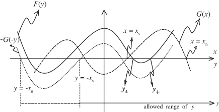
Figure 9: Shape of ${\cal G}(x)$ and ${\cal F}(y)$ for a general non-extremal charged massive hyperbolic AdS C-metric studied in section V.3. The allowed range of $x$ is between $x_{\mathrm{s}}$ and $x_{\mathrm{n}}$ where ${\cal G}(x)$ is positive and compact. The permitted range of $y$ is $-x\leq y<+\infty$. The presence of an accelerated horizon is indicated by $y_{A}$ and the black hole horizon by $y_{+}$. In the anti-Nariai case considered in subsection V.3.1, $y_{A}$ and $y_{+}$ coincide. [For completeness we comment on a case not represented in the figure but discussed on the text: when $q=0$, the zero $x_{\mathrm{n}}$ of ${\cal G}(x)$ disappears, and ${\cal G}(x)$ grows monotonically from $x=x_{\mathrm{s}}$ into $x=+\infty$.]

V.3.1 The anti-Nariai C-metric

We are interested in a particular extreme hyperbolic AdS C-metric, for which $y_{A}=y_{+}$ (see Fig. 9), and let us label this degenerated horizon by $\rho$: $y_{A}=y_{+}\equiv\rho$. In this case, the function ${\cal F}(y)$ can be written as

$${\cal F}(y)=-\frac{\rho^{2}-3\gamma}{\rho^{4}}(y-y_{\rm neg})(y-y^{\prime}_{\rm neg})(y-\rho)^{2}\>,$$ (84)

where

$$\gamma=\frac{|\Lambda|+3A^{2}}{3A^{2}}\>,$$ (85)

and the degenerate root $\rho$, and the negative roots $y_{\rm neg}$ and $y^{\prime}_{\rm neg}$ are given by

$$\rho=\frac{3m}{4q^{2}A}\left(1+\sqrt{1+\frac{8}{9}\frac{q^{2}}{m^{2}}}\>\right)\>,$$

$$y_{\rm neg}=-\frac{\gamma\rho}{3\gamma-\rho^{2}}\left(1+\sqrt{\frac{\rho^{2}-2\gamma}{\gamma}}\>\right)\>,$$

$$y^{\prime}_{\rm neg}=-\frac{\gamma\rho}{3\gamma-\rho^{2}}\left(1-\sqrt{\frac{\rho^{2}-2\gamma}{\gamma}}\>\right)\>.$$ (86)

The mass parameter and the charge parameter of the solution are written as a function of $\rho$ as

$$m=-\frac{1}{A\rho}\left(1-\frac{2\gamma}{\rho^{2}}\right)\>,$$

$$q^{2}=\frac{1}{A^{2}\rho^{2}}\left(\frac{3\gamma}{\rho^{2}}-1\right)\>.$$ (87)

The requirement that $y_{\rm neg}$ and $y^{\prime}_{\rm neg}$ are real roots and the condition $q^{2}\geq 0$ require that the allowed range of $\rho$ is

$$2\gamma<\rho^{2}\leq 3\gamma\>.$$ (88)

The mass and the charge of the anti-Nariai type solution, $m_{\rm aN}$ and $q_{\rm aN}$, respectively, are both monotonically decreasing functions of $\rho$, and as one comes from $\rho=\sqrt{3\gamma}$ into $\rho=\sqrt{2\gamma}$ one has,

$$-\frac{1}{3}\frac{1}{\sqrt{|\Lambda|+3A^{2}}}\leq m_{\rm aN}<0\>,$$

$$0\leq q_{\rm aN}<\frac{\sqrt{3}}{2}\frac{1}{\sqrt{|\Lambda|+3A^{2}}}\>.$$ (89)

In order to generate the anti-Nariai C-metric from the near-extreme topological AdS C-metric we first set

$$y_{A}=\rho-\varepsilon,\>\>\>\>y_{+}=\rho+\varepsilon,\>\>\>\>\>\>{\rm with}\>\>\varepsilon<<1\>,$$ (90)

in order that $\varepsilon$ measures the deviation from degeneracy, and the limit $y_{A}\rightarrow y_{+}$ is obtained when $\varepsilon\rightarrow 0$. Now, we introduce a new time coordinate $\tau$ and a new radial coordinate $\chi$,

$$t=\frac{1}{\varepsilon{\cal K}}\,\tau\>,\>\>\>\>\>\>\>\>\>\>\>y=\rho+\varepsilon\cosh\chi\>,$$ (91)

where

$$\!\!\!{\cal K}=\frac{3\gamma-\rho^{2}}{\rho^{4}}(\rho-y_{\rm neg})(\rho-y^{\prime}_{\rm neg})=\frac{2(|\Lambda|+3A^{2})}{A^{2}\rho^{2}}-1\>,$$

(92)

and $2\gamma<\rho^{2}\leq 3\gamma$ implies $1\leq{\cal K}<2$ with $q=0\Rightarrow{\cal K}=1$. In the limit $\varepsilon\rightarrow 0$, from Eq. (25) and Eq. (84), the metric becomes

$$ds^{2} = \frac{{\cal R}^{2}(x)}{{\cal K}}\left(-\sinh^{2}\chi\,d\tau^{2}+d\chi^{2}\right)$$ (93)

$$+{\cal R}^{2}(x)\left[{\cal G}^{-1}(x)dx^{2}+{\cal G}(x)dz^{2}\right]\>.$$

where

$${\cal R}^{2}(x)=\left(Ax+\sqrt{\frac{2(|\Lambda|+3A^{2})}{1+{\cal K}}}\right)^{-2}\>,$$ (94)

$$\!\!\!{\cal G}(x)=-1+x^{2}+\frac{A}{3}\sqrt{\frac{2(1+{\cal K})(2-{\cal K})^{2}}{(|\Lambda|+3A^{2})}}\,x^{3}+\frac{A^{2}}{4}\frac{{\cal K}^{2}-1}{|\Lambda|+3A^{2}}\,x^{4}\>,$$

(95)

Under the coordinate transformation (91), the Maxwell field for the magnetic case is still given by Eq. (27), while in the electric case, (28) becomes

$$F=-\frac{q}{{\cal K}}\,\sinh\chi\,d\tau\wedge d\chi\>.$$ (96)

The Carter-Penrose diagram of the anti-Nariai C-metric is also given by Fig. 4.(b).

At this point, let us focus our attention on the angular surfaces with $\tau=$constant and $\chi=$constant. When $q\neq 0$, we choose $x$ such that it belongs to the range $[x_{\mathrm{s}},x_{\mathrm{n}}]$ (sketched in Fig. 9) where ${\cal G}(x)\geq 0$. In this way, the metric has the correct signature, the angular surfaces are compact, and the allowed range of $y$ includes the acceleration ($y_{A}$) and black hole ($y_{+}$) horizons (if we had chosen the other possible interval of $x$ where ${\cal G}(x)\geq 0$, sketched in Fig. 9, this last condition would not be satisfied). We unavoidably have a conical singularity at least at one of the poles of this compact surface (that we label by $\tilde{S}^{2}$, say). Thus, the charged anti-Nariai C-metric has a compact angular surface of fixed size with a conical singularity at one of its poles. It is topologically conformal to $AdS_{2}\times\tilde{S}^{2}$. When $q=0$, the zero $x_{\mathrm{n}}$ of ${\cal G}(x)$ disappears, and ${\cal G}(x)$ grows monotonically from $x=x_{\mathrm{s}}$ into $x=+\infty$. Then, the angular surfaces are not compact, and we have a single pole ($x=x_{\mathrm{s}}$) with a conical singularity, which can be eliminated. Thus, the neutral anti-Nariai C-metric has a non-compact angular surface of fixed size (a kind of a deformed 2-hyperboloid that we label by $\tilde{H}_{2}$, say) which is free of conical singularities. It is topologically conformal to $AdS_{2}\times\tilde{H}_{2}$.

In order to obtain the $A=0$ limit, we first set $\hat{\rho}=A\rho$ [see first relation of (86)], a parameter that has a finite and well-defined value when $A\rightarrow 0$. Then when $A\rightarrow 0$ we have ${\cal K}\rightarrow{\cal K}_{0}=2|\Lambda|/\hat{\rho}^{2}-1$ and ${\cal R}^{2}\rightarrow{\cal R}_{0}^{\>2}=\hat{\rho}^{-2}$, with ${\cal R}_{0}^{\>2}$ and ${\cal K}_{0}$ satisfying relations (20). Moreover, when we set $A=0$, $m\neq 0$ and $q\neq 0$, the coordinate transformations $\theta=\int_{x_{\mathrm{s}}}^{x}{\cal{G}}^{-1/2}dx$ and $\phi=z$ imply that $x\in[x_{\mathrm{s}}=+1,+\infty[$, $x=\cosh\theta$, and ${\cal G}=-1+x^{2}=\sinh^{2}\theta$. The angular surface then reduces to a 2-hyperboloid, $H_{2}$, of fixed size with line element $d\theta^{2}+\sinh^{2}{\theta}\,d\phi^{2}$. Therefore, when $A=0$ the anti-Nariai C-metric reduces to the anti-Nariai solution (LABEL:qNariai-a) described in subsection II.3, with topology $AdS_{2}\times H_{2}$. The limiting procedure that has been applied in this subsection has generated a new exact solution that satisfies the Maxwell-Einstein equations in a negative cosmological constant background.

V.3.2 Other extremal limits

We could also discuss other extremal limits of the charged topological AdS C-metric (see Fig. 9), but these do not seem to be so interesting.

VI Conclusions

Following the limiting approach first introduced by Ginsparg and Perry GinsPerry , we have analyzed the extremal limits of the dS, flat and AdS C-metrics. Among other new exact solutions, we have generated the Nariai C-metric, the Bertotti-Robinson C-metric, the Nariai Bertotti-Robinson C-metric and the anti-Nariai C-metric. These solutions are the C-metric counterparts of the well know solutions found in the 1950’s. They are specified by an extra parameter: the acceleration parameter $A$ of the C-metric from which they are generated. When we set $A=0$ the solutions found in this paper reduce to the Nariai, the Bertotti-Robinson, the Nariai Bertotti-Robinson and the anti-Nariai solutions.

One of the features of these $A=0$ solutions is the fact that they are topologically the direct product of two 2-dimensional manifolds of constant curvature. Their C-metric counterparts are conformal to this topology, with the conformal factor depending on the angular coordinate. Moreover, the angular surfaces of these new C-solutions have a fixed size, but they lose the symmetry of the $A=0$ counterparts. For example, while the angular surfaces of the Nariai and Bertotti-Robinson solutions are round 2-spheres, the angular surfaces of their C-metric counterparts are deformed 2-spheres - they are compact but not round. Another important difference between the $A=0$ and $A\neq 0$ solutions is the fact that the $A\neq 0$ solutions have, in general, a conical singularity at least at one of the poles of their angular surfaces. This conical singularity is a reminiscence of the conical singularity that is present in the C-metric from which they were generated. In the C-metric these conical singularities are associated to the presence of a strut or string that furnishes the acceleration of the near-extremal black holes. In this context, we find that the Nariai C-metric generated from a extremal limit of the dS C-metric describes a spacetime that is conformal to the product $dS_{2}\times\tilde{S}^{2}$. To each point in the deformed 2-sphere corresponds a $dS_{2}$ spacetime, except for one point which corresponds a $dS_{2}$ spacetime with an infinite straight strut or string, with a mass density and pressure satisfying $p=-\mu$. Analogously, the Nariai Bertotti-Robinson dS C-metric describes a spacetime that is conformal to the product ${\mathbb{M}}^{1,1}\times\tilde{S}^{2}$. To each point in the deformed 2-sphere corresponds a ${\mathbb{M}}^{1,1}$ spacetime, except for one point which corresponds a ${\mathbb{M}}^{1,1}$ spacetime with an infinite straight strut or string. In the case of the Bertotti-Robinson dS C-metric (topologically conformal to $AdS_{2}\times\tilde{S}^{2}$), the strut or string does not survive to the Ginsparg-Perry limiting procedure, and thus in the end of the process we only have a conical singularity.

In what concerns the causal structure, the Carter-Penrose diagrams of the $A\neq 0$ solutions are equal to those of the $A=0$ solutions. For example, the diagram of the Nariai C-metric is equal to the one that describes the (1+1)-dimensional dS solution, the diagram of the Bertotti-Robinson C-metric and of the anti-Nariai C-metric is equal to the one that describes the (1+1)-dimensional AdS solution, and the diagram of the Nariai Bertotti-Robinson C-metric is given by the Rindler diagram.

Some of these solutions, perhaps all, are certainly of physical interest. Indeed, it is known that the Nariai solution ($A=0$) is unstable and, once created, it decays through the quantum tunnelling process into a slightly non-extreme black hole pair Bousso60y . We then expect that the Nariai C-metric is also unstable and that it will decay into a slightly non-extreme pair of black holes accelerated by a strut or by a string. The solutions found in this paper also play an important role in the decay of the dS or AdS spaces, and therefore can mediate the Schwinger-like quantum process of pair creation of black holes. Indeed, the Nariai, and the dS Nariai Bertotti-Robinson instantons ($A=0$) are one of the few Euclidean solutions that are regular, and have thus been used MelMosRom ; MannRoss ; BooMann ; VolkovWipf to study the pair creation of dS black holes materialized and accelerated by the cosmological constant background field (an instanton is a solution of the Euclidean field equations that smoothly connects the spacelike sections of the initial state, the pure dS space in this case, and the final state, the dS black hole pair in this case). Moreover, the Euclidean “Nariai” flat C-metric flatPC and Ernst solution DGKT ; ErnstPC (also discussed in this paper) have been used to analyze the process of pair production of $\Lambda=0$ black holes, accelerated by a string or by an electromagnetic external field, respectively. Therefore, its natural to expect that the Euclidean extremal limits of the dS C-metric and AdS C-metric found in this paper mediate the process of pair creation of black holes in a cosmological background, that are then accelerated by a string, in addition to the cosmological field acceleration. For the Nariai case, e.g., the picture would be that of the nucleation, in a dS background, of a Nariai C universe, whose string then breaks down and a pair of dS black holes is created at the endpoints of the string. This expectation is confirmed in OscLem-PCdS .

Appendix A $\Lambda=0$ limit of the Nariai and anti-Nariai solutions

In this appendix we find the $\Lambda=0$ limit of the Nariai solution, Eq. (2), and of the anti-Nariai solution, Eq. (LABEL:qNariai-a). In this limit the line element of both solutions goes apparently to infinity since ${\cal R}_{0}^{\>2}\rightarrow\infty$. To achieve the suitable limit of the Nariai solution, we first make the coordinate rescales: $\tilde{x}=({\cal R}_{0}/\sqrt{{\cal K}_{0}})\chi$, and $\varrho={\cal R}_{0}\,\theta$. Then, taking the $\Lambda=0$ limit, the solution becomes

$$ds^{2}=(-\tilde{x}^{2}d\tau^{2}+d\tilde{x}^{2})+(d\varrho^{2}+\varrho^{2}\,d\phi^{2})\,.$$ (97)

The spacetime sector is a Rindler factor, and the angular sector is a cylinder. Therefore, under the usual coordinate transformation $\tilde{x}=\sqrt{\bar{x}^{2}-\bar{t}^{2}}$ and $\tau={\rm arctanh(\bar{t}/\bar{x})}$, and unwinding the cylinder ($\bar{y}=\varrho\,\cos\phi$ and $\bar{z}=\varrho\,\sin\phi$), we have

$$ds^{2}=(-d\bar{t}^{\,2}+d\bar{x}^{2})+(d\bar{y}^{2}+d\bar{z}^{2})\,.$$ (98)

Therefore, while the Nariai C-metric is topologically $dS_{2}\times S^{2}$, its $\Lambda=0$ limit is topologically ${\mathbb{M}}^{1,1}\times{\mathbb{R}}^{2}$, i.e., ${\mathbb{R}}^{4}$.

A similar procedure shows that taking the $\Lambda=0$ limit of the anti-Nariai solution (LABEL:qNariai-a) ($AdS_{2}\times H_{2}$) leads to Eq. (98).

Appendix B Determination of the north and south poles

In this appendix we discuss the zeros of the function ${\cal G}(x)$ that appears in the extremal limits of the dS C-metric, and in the extremal limits of the flat C-metric. This function ${\cal G}(x)$ has only two real zeros in the cases discussed in this paper, namely the Nariai, the Bertotti-Robinson, and the Nariai Bertotti-Robinson (both for $\Lambda>0$ and $\Lambda=0$). These two roots are the south pole and the north pole, and are respectively given by

$$x_{\mathrm{s}} = -p+\frac{h}{2}-\frac{a}{4\,b}<0\,,$$

$$x_{\mathrm{n}} = +p+\frac{h}{2}-\frac{a}{4\,b}>0\>,$$ (99)

with

$$p = \frac{1}{2}\left(-\frac{s}{3}+\frac{a^{2}}{2\,b^{2}}-\frac{1-12\,b}{3\,s\,b^{2}}-\frac{4}{3\,b}+n\right)^{1/2}\>,$$

$$n = \frac{-a^{3}+4\,a\,b}{4\,h\,b^{3}}\>,$$

$$h = \sqrt{\frac{s}{3}+\frac{a^{2}}{4\,b^{2}}+\frac{1-12\,b}{3\,s\,b^{2}}-\frac{2}{3\,b}}\>,$$

$$s = \frac{1}{2^{1/3}\,b}\left(\lambda-\sqrt{\lambda^{2}-4(1-12\,b)^{3}}\right)^{1/3}\>,$$

$$\lambda = 2-27\,a^{2}+72\,b\>,$$ (100)

where $a$ and $b$ are, respectively, the absolute values of the coefficients of $x^{3}$ and $x^{4}$ in Eqs. (42), (53), (61), (71), and (72). For the function ${\cal G}(x)$ written in a different polynomial form that facilitates the determination of its zeros see Hong and Teo HongTeo .

References

- (1) S. F. Hawking, G. F. R. Ellis, The Large Scale Structure of Space-Time, (Cambridge University Press, 1976).
- (2) B. Carter, General theory of statinary black holes, in Black holes edited by B. DeWitt and C. DeWitt (Gordon and Breach, New York, 1973).
- (3) D. Kramer, H. Stephani, M. MacCallum, E. Herlt, Exact solutions of Einstein’s Field Equations, (Cambridge University Press, 1980).
- (4) H. Nariai, On some static solutions of Einstein’s gravitational field equations in a spherically symmetric case, Sci. Rep. Tohoku Univ. 34, 160 (1950); On a new cosmological solution of Einstein’s field equations of gravitation, Sci. Rep. Tohoku Univ. 35, 62 (1951).
- (5) H. Nariai, H. Ishihara, On the de Sitter and Nariai solutions in General Relativity and their extension in higher dimensional spacetime, in A Random Walk in Relativity and Cosmology, edited by P. N. Dadhich, J. K. Rao, J. V. Narlikar, C. V. Vishveshwara (John Wiley Sons, New York).
- (6) B. Bertotti, Uniform electromagnetic field in the theory of general relativity, Phys. Rev. 116, 1331 (1959); I. Robinson, Bull. Acad. Polon. 7, 351 (1959).
- (7) M. Caldarelli, L. Vanzo, Z. Zerbini, The extremal limit of D-dimensional black holes, in Geometrical Aspects of Quantum Fields, edited by A. A. Bytsenko, A. E. Gonçalves, B. M. Pimentel (World Scientific, Singapore, 2001); hep-th/0008136; N. Dadhich, On product spacetime with 2-sphere of constant curvature, gr-qc/0003026.
- (8) P. Ginsparg, M. J. Perry, Semiclassical perdurance of de Sitter space, Nucl. Phys. B 222, 245 (1983).
- (9) R. Bousso, Adventures in de Sitter space, hep-th/0205177.
- (10) W. Kinnersley, M. Walker, Uniformly accelerating charged mass in General Relativity, Phys. Rev. D 2, 1359 (1970).
- (11) O. J. C. Dias, J. P. S. Lemos, Pair of accelerated black holes in de Sitter background: the dS C-metric, Phys. Rev. D 67, 084018 (2003).
- (12) O. J. C. Dias, J. P. S. Lemos, Pair of accelerated black holes in an anti-de Sitter background: the AdS C-metric, Phys. Rev. D 67, 064001 (2003).
- (13) M. Ortaggio, Impulsive waves in the Nariai universe, Phys. Rev. D 65, 084046 (2002).
- (14) R. Bousso, S. W. Hawking, The probability for primordial black holes, Phys. Rev. D 52, 5659 (1995); Pair production of black holes during inflation, Phys. Rev. D 54, 6312 (1996).
- (15) S. W. Hawking, S. F. Ross, Duality between electric and magnetic black holes, Phys. Rev. D 52, 5865 (1995).
- (16) R. B. Mann, S. F. Ross, Cosmological production of charged black hole pairs, Phys. Rev. D 52, 2254 (1995).
- (17) R. Bousso, Charged Nariai black holes with a dilaton, Phys. Rev. D 55, 3614 (1997).
- (18) R. Bousso, S. W. Hawking, (Anti-)evaporation of Schwarzschild-de Sitter black holes, Phys. Rev. D 57, 2436 (1998); R. Bousso, Proliferation of de Sitter space, Phys. Rev. D 58, 083511 (1998).
- (19) S. Nojiri, S. D. Odintsov, Quantum evolution of Schwarzschild-de Sitter (Nariai) black holes, Phys. Rev. D 59, 044026 (1999); De Sitter space versus Nariai black hole: stability in d5 higher derivative gravity, Phys. Lett. B 523, 165 (2001).
- (20) L. A. Kofman, V. Sahni, A. A. Starobinski, Anisotropic cosmological model created by quantum polarization of vacuum, Sov. Phys. JETP 58, 1090 (1983).
- (21) F. Mellor, I. Moss, Black holes and quantum wormholes, Phys. Lett. B 222, 361 (1989); Black holes and gravitational instantons, Class. Quant. Grav. 6, 1379 (1989); L. J. Romans, Supersymmetric, cold and lukewarm black holes in cosmological Einstein-Maxwell theory, Nucl. Phys. B 383, 395 (1992).
- (22) I. S. Booth, R. B. Mann, Cosmological pair production of charged and rotating black holes, Nucl. Phys. B 539, 267 (1999).
- (23) M. Volkov, A. Wipf, Black hole pair creation in de Sitter space: a complete one-loop analysis, Nucl. Phys. B582, 313 (2000).
- (24) A. J. M. Medved, Nearly degenerated dS horizons from a 2-D perpective, hep-th/0302058.
- (25) A. S. Lapedes, Euclidean quantum field theory and the Hawking effect, Phys. Rev. D 17, 2556 (1978).
- (26) O. B. Zaslavsky, Geometry of nonextreme black holes near the extreme state, Phys. Rev. D 56, 2188 (1997); Entropy of quantum fields for nonextreme black holes in the extreme limit, Phys. Rev. D 57, 6265 (1998).
- (27) R. B. Mann, S. N. Solodukhin, Universality of quantum entropy for extreme black holes, Nucl. Phys. B 523, 293 (1998).
- (28) D. J. Navarro, J. Navarro-Salas, P. Navarro, Holography, degenerated horizons and entropy, Nucl. Phys. B 580, 311 (2000); A. J. M. Medved, Reissner-Nordström Near extremality from a Jackiw-Teiltelboim perpective, hep-th/0111091. A. Barvinsky, S. Das, G. Kunstatter, Quantum mechanics of charged black holes, Phys. Lett. B 517, 415 (2001).
- (29) M. Ortaggio, J. Podolský, Impulsive waves in electrovac direct product spacetimes with Lambda, Class. Quantum Grav. 19, 5221 (2002).
- (30) J. P. S. Lemos, Cylindrical black hole in general relativity, Phys. Lett. B353, 46 (1995); J. P. S. Lemos, V. T. Zanchin, Rotating charged black strings in general relativity, Phys. Rev. D54, 3840 (1996); O. J. C. Dias, J. P. S. Lemos, Magnetic strings in anti-de Sitter general relativity, Class. Quantum Grav. 19, 2265 (2002).
- (31) S. Åminnenborg, I. Bengtsson, S. Holst, P. Peldán, Making anti-de Sitter black holes, Class. Quantum Grav. 13, 2707 (1996); D. R. Brill, Multi-black holes in 3D and 4D anti-de Sitter spaces, Helv. Phys. Acta 69, 249 (1996); S. L. Vanzo, Black holes with unusual topology, Phys. Rev. D 56, 6475 (1997); D. R. Brill, J. Louko, P. Peldán, Thermodynamics of (3+1)-dimensional black holes with toroidal or higher genus horizons, Phys. Rev. D 56, 3600 (1997); R. B. Mann, Black holes of negative mass, Class. Quantum Grav. 14, 2927 (1997); S. Holst, P. Peldan, Black holes and causal structure in anti-de Sitter isometric spacetimes, Class. Quantum Grav. 14, 3433 (1997).
- (32) J. F. Plebański, M. Demiański, Rotating, charged and uniformly accelerating mass in general relativity, Annals of Phys. (N.Y.) 98, 98 (1976).
- (33) J. Podolský, J.B. Griffiths, Uniformly accelerating black holes in a de Sitter universe, Phys. Rev. D 63, 024006 (2001).
- (34) J. Bičák, P. Krtouš, Accelerated sources in de Sitter spacetime and the insuffiency of retarded fields, Phys. Rev. D 64, 124020 (2001); The fields of uniformly accelerated charges in de Sitter spacetime, Phys. Rev. Lett. 88, 211101 (2002).
- (35) P. Krtouš, J. Podolský, Radiation from accelerated black holes in de Sitter universe, gr-qc/0301110.
- (36) J. Maldacena, J. Michelson, A. Strominger, Anti-de Sitter fragmentation, JHEP 9902:11, (1999); Vacuum states for black holes, M. Spradlin, A. Strominger, JHEP 9911:021, (1999).
- (37) O. J. C. Dias, J. P. S. Lemos, Pair creation of de Sitter black holes on cosmic strings, to be submitted (2003).
- (38) S. W. Hawking, S. F. Ross, Pair production of black holes on cosmic strings, Phys. Rev. Lett. 75, 3382 (1995); R. Emparan, Pair production of black holes joined by cosmic strings, Phys. Rev. Lett. 75, 3386 (1995); D. M. Eardley, G. T. Horowitz, D. A. Kastor, J. Traschen, Breaking cosmic strings without monopoles, Phys. Rev. Lett. 75, 3390 (1995); R. Gregory, M. Hindmarsh, Smooth metrics for snapping strings, Phys. Rev. D 52, 5598 (1995); A. Achúcarro, R. Gregory, K. Kuijken, Abelian Higgs hair for black holes, Phys. Rev. D 52, 5729 (1995).
- (39) D. Garfinkle, S. B. Giddings, A. Strominger, Entropy in black hole pair production, Phys. Rev. D 49, 958 (1994); H. F. Dowker, J. P. Gauntlett, S. B. Giddings, G. T. Horowitz, Pair creation of extremal black holes and Kaluza-Klein monopoles, Phys. Rev. D 50, 2662 (1994); S. W. Hawking, G. T. Horowitz, S. F. Ross, Entropy, area, and black hole pairs, Phys. Rev. D 51, 4302 (1995).
- (40) H. F. Dowker, J. P. Gauntlett, D. A. Kastor, J. Traschen, Pair creation of dilaton black holes, Phys. Rev. D 49, 2909 (1994).
- (41) J. Bičák, Gravitational radiation from uniformly accelerated particles in general relativity, Proc. Roy. Soc. A 302, 201 (1968); V. Pravda, A. Pravdova, Boost-rotation symmetric spacetimes - review, Czech. J. Phys. 50, 333 (2000); On the spinning C-metric, in Gravitation: Following the Prague Inspiration, edited by O. Semerák, J. Podolský, M. Zofka (World Scientific, Singapore, 2002), gr-qc/0201025.
- (42) F. J. Ernst, Removal of the nodal singularity of the C-metric, J. Math. Phys. 17, 515 (1976).
- (43) J. D. Brown, Black hole pair creation and the entropy factor, Phys. Rev. D 51, 5725 (1995).
- (44) G. T. Horowitz, H. J. Sheinblatt, Tests of cosmic censorship in the Ernst spacetime, Phys. Rev. D 55, 650 (1997).
- (45) R. Emparan, G. T. Horowitz, R. C. Myers, Exact description of black holes on branes, JHEP 0001 007 (2000); Exact description of black Holes on branes II: Comparison with BTZ black holes and black strings, JHEP 0001 021 (2000); J. Podolský, Accelerating black holes in anti-de Sitter universe, Czech. J. Phys. 52, 1 (2002).
- (46) R. Mann, Pair production of topological anti-de Sitter black holes, Class. Quantum Grav. 14, L109 (1997); Charged topological black hole pair creation, Nucl. Phys. B 516, 357 (1998).
- (47) K. Hong, E. Teo, A new form of the C-metric, gr-qc/0305089.