hep-th/0306189

UT-03-22 June, 2003

Boundary states as exact solutions
of (vacuum) closed string field theory

Isao Kishimoto, Yutaka Matsuo and Eitoku Watanabe

Department of Physics, Faculty of Science, University of Tokyo
Hongo 7-3-1, Bunkyo-ku, Tokyo 113-0033, Japan

We show that the boundary states are idempotent $B*B=B$ with respect to the star product of HIKKO type closed string field theory. Variations around the boundary state correctly reproduce the open string spectrum with the gauge symmetry. We explicitly demonstrate it for the tachyonic and massless vector modes. The idempotency relation may be regarded as the equation of motion of closed string field theory at a possible vacuum.

1 Introduction

Study of the off-shell structure of string theory is an essential step in understanding its non-perturbative physics. In recent years, Witten-type open string field theory [1] has been intensively examined in this context. One of the goals is to understand D-branes as soliton solutions of open string field theory. One of the promising discoveries was that the energy of the tachyon vacuum correctly reproduced the tension of D-branes at least numerically.[2]

Inspired by the experiences of noncommutative field theory, it was conjectured by Rastelli, Sen and Zwiebach that the D-branes may be understood as the solutions to the projector equation,

$$\Psi\star\Psi=\Psi\,\,,$$ (1.1)

where $\star$ is the noncommutative and associative Witten-type star product for an open string field. It was conjectured that this equation may be understood as the equation of motion of a string field expanded around the tachyon vacuum (the so-called vacuum string field theory (VSFT) conjecture [3][4]). In particular, a few examples of the projectors, the sliver state or butterfly state, were examined as the candidates which describe the D-brane.

It turned out, however, that the treatment of D-branes in open string field theory is very delicate. One of the difficulties was the description of the closed string sector. In Witten-type open string field theory, the action does not include the closed string degrees of freedom at the tree level. If we need to describe them in open string language alone, we have to consider a singular state such as identity string field where the closed string vertex is inserted at the midpoint.[5][6][4] The midpoint in open string field theory causes many subtleties, for example, it causes the breakdown of the associativity [7] and we have to be very careful while handling such a degree of freedom. D-brane couples to the closed string sector (for example, gravity) at the tree level, and we cannot escape from using such a singular description. The level truncation regularization seems to handle it numerically. However, the analytic treatment of the problem remains as a real challenge.

In this paper, we change the viewpoint and start the analysis of D-branes in closed string field theory. We believe that such a treatment is natural since the nature of D-branes is most precisely encoded in the boundary state $|B\rangle$ which lives in the Hilbert space of the closed string sector. In particular, we will prove that the boundary states (both for Neumann and Dirichlet boundary conditions) satisfy an analogue of Eq.(1.1),

$$|B\rangle*|B\rangle=|B\rangle\,\,$$ (1.2)

up to a pure ghost prefactor.

Unlike the open string version, Eq.(1.2) has a natural geometrical meaning. The boundary state, as suggested by its name, describes the boundary condition of the string world sheet. Suppose there exist two holes with the same type of boundary condition. If we merge these two holes by a closed string star product, we expect to have the same boundary condition on the new hole.(Fig.1)

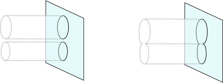
Figure 1: $*$ product of the boundary states

To demonstrate this observation explicitly, we have to be specific about the choice of the star product. There are three candidates of closed string field theory which were well examined so far.

The oldest one is the light-cone gauge approach [9]. This is consistent in the sense that it produces the correct integration range over the moduli parameter. However, for the application to our problem, it is not useful since the boundary states have nontrivial dependence on the time coordinate. We need covariant descriptions.

The second one is the closed string version of Witten’s open string theory. A generalization of Witten-type midpoint interaction vertex to closed strings results in nonpolynomial string field theory [10, 11]. The action contains infinitely many terms to cover the moduli spaces for the Riemann surfaces corresponding to various interactions. This approach contains many mathematically interesting features such as $L_{\infty}$ structure. Handling of the moduli parameters still remains as a challenge, however, and it has not reached the completely satisfactory level.

The third one is based on a split-joining type vertex, which was proposed about the same time as Witten-type open string field theory and is now known as HIKKO’s (Hata-Itoh-Kugo-Kunitomo-Ogawa) string field theory [13, 14]. It has exactly the same action as Witten’s open string field theory, namely, the kinetic term and a three string interaction. In HIKKO’s theory, it is necessary to introduce a parameter called string length $\alpha$ to specify string interactions, which has no analogue in Witten-type string field theories. It must be integrated in computing physical quantities and might cause a divergence in loop amplitudes [15]. The simplest way to resolve this difficulty is to just set $\alpha=p^{+}$, but it breaks the covariance.

To summarize, there is no completely satisfactory closed string field theory. In this paper, we adopt HIKKO’s star product to explicitly demonstrate Eq.(1.2). However, we expect it to hold even if we replace it with a Witten-type product. We will come back to prove it in our future paper [16]. We would like to propose this relation as a universal characterization of the boundary states in closed string field theory, which is independent of the specific proposals for the action. A merit to use HIKKO’s approach is the analogy of the action with Witten’s open string field theory. If we want to have an analogy with VSFT proposal, this gives a good reason to start from it.

We note that HIKKO’s $*$ product in Eq.(1.2) has different properties compared with Witten’s star product in open string field theory. It may be summarized as the following relations:

$$\Phi*\Psi=-(-1)^{|\Phi||\Psi|}\Psi*\Phi\,\,,$$ (1.3)

$$(\Phi*\Psi)*\Lambda+(-1)^{|\Phi|(|\Psi|+|\Lambda|)}(\Psi*\Lambda)*\Phi+(-1)^{|\Lambda|(|\Phi|+|\Psi|)}(\Lambda*\Phi)*\Psi=0\,\,,$$ (1.4)

$$Q(\Phi*\Psi)=Q\Phi*\Psi+(-1)^{|\Phi|}\Phi*Q\Psi\,\,.$$ (1.5)

First of all, the product is (anti-)commutative (1.3). While it breaks associativity, it satisfies the analogue of Jacobi identity (1.4). In a sense, it has the same property as the commutator of Witten-type open string product, $\Phi*^{HIKKO}\Psi\leftrightarrow\Phi\star^{Witten}\Psi-(-1)^{|\Phi||\Psi|}\Psi\star^{Witten}\Phi\,\,.$ Since the nature of the product is different, we cannot interpret the equation (1.2) as defining a projector. In the following, however, we will continue to use the word “projector” to describe the state that satisfies Eq.(1.2) because of the similarity with the discussion of the open string.

We conjecture that Eq.(1.2) gives a good characterization of the conformal invariant boundary. For this purpose, we calculate an infinitesimal variation of the boundary state of the following form,

$$\delta_{V}|B\rangle=\oint d\sigma V(\sigma)|B\rangle$$ (1.6)

where $V(\sigma)$ is a vertex operator inserted at the boundary. We argue that the idempotency condition (1.2) requires the vertex $V$ to be marginal. We will prove this expectation for the tachyonic state and the massless vector state. For such variations, this gives the mass-shell condition for these open string modes. In a sense, the idempotency condition knows the mass-shell condition of the open string while they are the equation for the closed string states!

We note that our argument is very similar to the discussion of vacuum string field theory. For example, use of the variation of Eq.(1.2) to derive the mass-shell condition for the open string states was examined in the VSFT context by Hata-Kawano [17] and Okawa [18]. In particular, in the latter approach, the marginal deformation was made over the whole boundary. This is basically the same variation as Eq.(1.6). The difference is, of course, the Hilbert space where the projector lives. In VSFT, to describe such an projector, we have to consider singular states. For example, the sliver state is made by taking the infinite star products of the vacuum state. On the other hand, our closed string description does not include such a singular manipulation. The boundary state is a well-defined state in the boundary conformal field theory. In this way, we can escape from the subtleties of VSFT.

The paper is organized as follows. In section 2, we give the explicit definitions of the boundary states and the 3-string vertex which are discussed in this paper. We will then present our claims more precisely. The proof is given explicitly in the following sections which are rather technical. In section 3 we prove the idempotency relation of the boundary states. We need many properties of the Neumann coefficients which are summarized in appendix C. In section 4 we investigate infinitesimal variations around the boundary state and derive on-shell condition of open string on them. In section 5, we discuss some issues of our results.

2 Boundary state and star product of closed string field theory

2.1 Boundary states

The boundary states $|B(F)\rangle$ which we are going to discuss are those for D$p$-branes with constant field strength $F_{\mu\nu}$ [19],

$$|B(F)\rangle = e^{-\sum_{n\geq 1}a^{(+)\dagger}_{n}{\cal O}a^{(-)\dagger}_{n}}e^{\sum_{n\geq 1}(c^{(+)\dagger}_{n}\bar{c}^{(-)\dagger}_{n}+c^{(-)\dagger}_{n}\bar{c}^{(+)\dagger}_{n})}|p_{\mu}=0,x^{i}\rangle\,,$$ (2.3)

$${\cal O}^{\mu}_{~{}\nu}=\left[(1+F)^{-1}(1-F)\right]^{\mu}_{~{}\nu}\,,~{}~{}~{}\mu,\nu=0,1,\cdots,p\,,$$

$${\cal O}^{i}_{~{}j}=-\delta^{i}_{j}\,,~{}~{}~{}~{}i,j=p+1,\cdots,d-1\,\,\,.$$

$x^{\mu}\,(\mu=0,1,\cdots,p)$ are the coordinates along the Neumann directions and $x^{i}\,(i=p+1,\cdots,d-1)$ are along the Dirichlet directions. We use the letters $M,N$ ($=0,\cdots,d-1$) to represent all these directions. We put $d=26$ since we are considering bosonic string theory. These states satisfy the following conditions:

$$\sqrt{\pi}X^{i}(\sigma)|B(F)\rangle=x^{i}|B(F)\rangle\,,$$ (2.4)

$$\left(P_{\mu}(\sigma)-F_{\mu\nu}{d\over d\sigma}X^{\nu}(\sigma)\right)|B(F)\rangle=0\,,$$ (2.5)

$$\pi_{c}(\sigma)|B(F)\rangle=\pi_{\bar{c}}(\sigma)|B(F)\rangle=0\,.$$ (2.6)

The boundary states are invariant under BRST transformation $Q_{B}|B(F)\rangle=0$. ${\cal O}$ is orthogonal $\mathcal{O}\mathcal{O}^{T}=\mathcal{O}^{T}\mathcal{O}=1$ since $F_{\mu\nu}$ is antisymmetric. Along the Dirichlet directions, this matrix becomes trivial in the sense: $\left({1+{\cal O}\over 2}\right)^{i}_{~{}j}=0$, but zero modes have nonzero momentum. The oscillator representations of Eqs.(2.4–2.6) are summarized in the appendix D.

2.2 Reflector and 3-string vertex

HIKKO’s star product for the closed string is a covariant version of light-cone string field theory. It is defined by the reflector $\langle\tilde{R}|$ which maps a ket vector to a bra vector and the three string vertex $|V(1,2,3)\rangle$ which lives in the tensor product of three closed string Hilbert spaces :

$$|\Phi_{1}*\Phi_{2}\rangle_{3} = \int d\bar{c}^{(1)}_{0}d\bar{c}^{(2)}_{0}{}_{1}\langle\Phi_{1}|{}_{2}\langle\Phi_{2}|V(1,2,3)\rangle,$$ (2.8)

$${}_{2}\langle\Phi| := \int d\bar{c}_{0}^{(1)}\langle\tilde{R}(1,2)|\Phi\rangle_{1}\,\,.$$ (2.9)

The reflector is defined by [14]:

$$\langle\tilde{R}(1,2)| = \int d^{d}x^{(1)}d^{d}x^{(2)}{d\alpha_{1}d\alpha_{2}\over(2\pi)^{2}}{}_{1}\langle x^{(1)},\alpha_{1}|{}_{2}\langle x^{(2)},\alpha_{2}|$$ (2.10)

$$\times\exp\left[-\sum_{\pm,n\geq 1}\left(a_{n}^{(\pm)(1)}\cdot a_{n}^{(\pm)(2)}+c_{n}^{(\pm)(1)}\bar{c}_{n}^{(\pm)(2)}-\bar{c}_{n}^{(\pm)(1)}c_{n}^{(\pm)(2)}\right)\right]$$

$$\times\delta^{d}(x^{(1)}-x^{(2)})\delta(\bar{c}_{0}^{(1)}-\bar{c}_{0}^{(2)})2\pi\delta(\alpha_{1}+\alpha_{2})\,.$$

The 3-string vertex $|V(1,2,3)\rangle$ is given explicitly in terms of oscillators as

$$|V(1,2,3)\rangle=\int\delta(1,2,3)[\mu(1,2,3)]^{2}\wp^{(1)}\wp^{(2)}\wp^{(3)}$$

$$~{}~{}~{}~{}~{}~{}~{}~{}~{}~{}~{}~{}~{}~{}~{}~{}~{}~{}\times\prod_{r=1}^{3}\left(1+{1\over\sqrt{2}}w^{(r)}_{I}\bar{c}_{0}^{(r)}\right)e^{F(1,2,3)}|p_{1},\alpha_{1}\rangle_{1}|p_{2},\alpha_{2}\rangle_{2}|p_{3},\alpha_{3}\rangle_{3}\,,~{}~{}~{}~{}~{}$$ (2.11)

$$F(1,2,3)=\sum_{\pm}\sum_{r,s=1}^{3}\sum_{m,n\geq 1}\tilde{N}^{rs}_{mn}\left({1\over 2}\,a_{m}^{(\pm)(r)\dagger}\cdot a_{n}^{(\pm)(s)\dagger}+\sqrt{m}\alpha_{r}c^{(\pm)(r)\dagger}_{m}(\sqrt{n}\alpha_{s})^{-1}\bar{c}^{(\pm)(s)\dagger}_{n}\right)$$

$$~{}~{}~{}~{}~{}~{}~{}~{}~{}~{}~{}~{}~{}~{}~{}~{}+{1\over 2}\sum_{\pm}\sum_{r=1}^{3}\sum_{n\geq 1}\tilde{N}^{r}_{n}\,a^{(\pm)(r)\dagger}_{n}\cdot{\bf P}-{\tau_{0}\over 4\alpha_{1}\alpha_{2}\alpha_{3}}{\bf P}^{2}\,,$$ (2.12)

$${\bf P}:=\alpha_{1}p_{2}-\alpha_{2}p_{1}\,,$$ (2.13)

$$w_{I}^{(r)}={1\over\sqrt{2}}\sum_{\pm}\sum_{s=1}^{3}\sum_{m\geq 1}w^{rs}_{m}\alpha_{s}c^{(\pm)(s)\dagger}_{m}\,,~{}~{}~{}~{}w^{rs}_{m}=\chi^{rs}m\bar{N}^{s}_{m}+{1\over\alpha_{r}}\sum_{n=1}^{m-1}m\bar{N}^{ss}_{m-n,n}\,,$$ (2.14)

$$\chi^{rs}=\delta_{r,s}{1\over\alpha_{r}}(\alpha_{r-1}-\alpha_{r+1})+\sum_{t=1}^{3}\epsilon^{rst}\,,~{}~{}~{}~{}(\alpha_{4}:=\alpha_{1}\,,~{}~{}\epsilon^{123}=+1)$$ (2.15)

$$\mu(1,2,3)=\exp\left(-\tau_{0}\sum_{r=1}^{3}{1\over\alpha_{r}}\right)\,,~{}~{}~{}~{}~{}~{}\tau_{0}=\sum_{r=1}^{3}\alpha_{r}\log|\alpha_{r}|\,,$$ (2.16)

$$\int\delta(1,2,3)=\int{d^{d}p_{1}\over(2\pi)^{d}}{d^{d}p_{2}\over(2\pi)^{d}}{d^{d}p_{3}\over(2\pi)^{d}}{d\alpha_{1}\over 2\pi}{d\alpha_{2}\over 2\pi}{d\alpha_{3}\over 2\pi}(2\pi)^{d}\delta^{d}(p_{1}+p_{2}+p_{3})2\pi\delta(\alpha_{1}+\alpha_{2}+\alpha_{3})\,,~{}~{}~{}$$ (2.17)

$$\wp^{(i)}=\oint{d\theta\over 2\pi}\,e^{-i\theta(N_{+}^{(i)}-N_{-}^{(i)})}\,,~{}~{}~{}~{}N_{\pm}=\sum_{n\geq 1}n\left(a_{n}^{(\pm)\dagger}\cdot a_{n}^{(\pm)}+c_{n}^{(\pm)\dagger}\bar{c}_{n}^{(\pm)}+\bar{c}_{n}^{(\pm)\dagger}c_{n}^{(\pm)}\right)\,.$$ (2.18)

The coefficients $\tilde{N}^{rs}_{mn}$ are Neumann coefficients; $\tilde{N}_{mn}^{rs}:=\sqrt{m}\bar{N}_{mn}^{rs}\sqrt{n}\,,~{}\tilde{N}^{r}_{m}:=\sqrt{m}\bar{N}^{r}_{m}$. Their definitions and some formulae which they satisfy are given in appendix C. $\wp^{(i)}$ is a projector to impose the level matching condition $N_{+}=N_{-}$ on the $i$th string. Note that we can rewrite some of the above as

$${\bf P}=\alpha_{1}p_{2}-\alpha_{2}p_{1}=\alpha_{2}p_{3}-\alpha_{3}p_{2}=\alpha_{3}p_{1}-\alpha_{1}p_{3}\,,~{}~{}~{}-{{\bf P}^{2}\over 4\alpha_{1}\alpha_{2}\alpha_{3}}=\sum_{r=1}^{3}{p_{r}^{2}\over 4\alpha_{r}}$$ (2.19)

in the presence of $\delta$-functions which impose $p_{1}+p_{2}+p_{3}=0$ and $\alpha_{1}+\alpha_{2}+\alpha_{3}=0$.

The 3-string vertex $|V(1,2,3)\rangle$ is determined by the overlap conditions (Fig.2),

$$\Theta_{1}X^{(1)}(\sigma_{1})+\Theta_{2}X^{(2)}(\sigma_{2})-X^{(3)}(\sigma_{3})=0\,\,,$$ (2.20)

$$\Theta_{1}\alpha_{1}c^{(1)}(\sigma_{1})+\Theta_{2}\alpha_{2}c^{(2)}(\sigma_{2})-\alpha_{3}c^{(3)}(\sigma_{3})=0\,\,,$$ (2.21)

$$\Theta_{1}\alpha_{1}^{-2}\bar{c}^{(1)}(\sigma_{1})+\Theta_{2}\alpha_{2}^{-2}\bar{c}^{(2)}(\sigma_{2})-\alpha_{3}^{-2}\bar{c}^{(3)}(\sigma_{3})=0\,\,,$$ (2.22)

$$\Theta_{1}(\sigma)\equiv\theta(\pi|\alpha_{1}|-|\sigma|)\,,\Theta_{2}(\sigma)\equiv\theta(|\sigma|-\pi|\alpha_{1}|)\,,$$ (2.23)

$$\sigma_{1}(\sigma)=\frac{\sigma}{\alpha_{1}}\,,\quad\sigma_{2}(\sigma)=\frac{\sigma-\mathrm{sgn}(\sigma)\pi|\alpha_{1}|}{\alpha_{2}}\,,\quad\sigma_{3}(\sigma)=\frac{\mathrm{sgn}(\sigma)\pi|\alpha_{3}|-\sigma}{-\alpha_{3}}\,,$$ (2.24)

where $-\pi|\alpha_{3}|\leq\sigma\leq\pi|\alpha_{3}|$ and $\alpha_{i}$ ($i=1,2,3$) are real parameters with the constraint $\alpha_{1}+\alpha_{2}+\alpha_{3}=0$. In light-cone string field theory, they are interpreted as the light-cone momenta which are preserved at the interaction. In the covariant theory, they become the external parameters which characterize the overlap conditions (2.20–2.22). We note that the above conditions are for the particular case $|\alpha_{3}|=|\alpha_{1}|+|\alpha_{2}|$ and we need some modifications for other choices.

Figure 2: Overlapping configuration of three closed strings. Strings with the labels 1,2,3 whose length parameters are $|\alpha_{1}|,|\alpha_{2}|,|\alpha_{3}|(=|\alpha_{1}|+|\alpha_{2}|)$ are parametrized by $\sigma_{1},\sigma_{2},\sigma_{3}\,(-\pi\leq\sigma_{r}\leq\pi)$. $\sigma_{3}=\pm\pi(\beta+1)~{}~{}(\beta:=\alpha_{1}/\alpha_{3})$ are interaction points on string 3 which correspond to $\sigma_{1}=\pm\pi,\sigma_{2}=0$ on string 1 and 2, respectively.

2.3 Main results

At this point, it is possible to make a precise statement of our results, given as follows.

1. We slightly redefine the boundary state $|B(F)\rangle$ (i) by multiplying $\bar{c}_{0}$ to obtain the correct ghost number of closed string field in the physical sector in gauge-fixed action [14] and (ii) by including the string-length parameter ($\alpha$ parameter)

   $$|\Phi_{B}(\alpha)\rangle = e^{-a^{(+)\dagger}{\cal O}a^{(-)\dagger}}e^{c^{(+)\dagger}\bar{c}^{(-)\dagger}+c^{(-)\dagger}\bar{c}^{(+)\dagger}}\bar{c}_{0}|p_{\mu}=0,x^{i},\alpha\rangle\,\,.$$ (2.25)

   We claim that it satisfies the following relation (“projector equation” with the ghost insertion):

   $$|\Phi_{B}(\alpha_{1})*\Phi_{B}(\alpha_{2})\rangle=c_{B}|\Phi_{B}(\alpha_{1}+\alpha_{2})\rangle\,,~{}~{}~{}~{}~{}~{}~{}~{}~{}\alpha_{1}\alpha_{2}>0\,,$$ (2.26)

   $$c_{B}\equiv V_{d-p-1}\,{{c}}\,\frac{\partial}{\partial\bar{c}_{0}}\,\,,$$ (2.27)

   $${{c}}\equiv e^{-2(\beta^{2}+\beta+1)\left({\log|\beta|\over\beta+1}-{\log|\beta+1|\over\beta}\right)}\left(\det(1-r^{2})\right)^{-(d-2)/2}\,,~{}~{}~{}~{}~{}\beta\equiv-\frac{\alpha_{1}}{\alpha_{1}+\alpha_{2}}\,.$$ (2.28)

   $V_{d-p-1}$ is the volume of the Dirichlet directions. The matrix $r$ is given by,

   $$r_{mn}=\frac{\beta(\beta+1)(mn)^{3/2}}{m+n}\bar{f}^{(3)}_{m}\bar{f}^{(3)}_{n}\,,\quad\bar{f}^{(3)}_{m}=\frac{\Gamma(-m\beta)e^{m(\beta\log|\beta|-(\beta+1)\log|\beta+1|)}}{m!\,\Gamma(-m\beta+1-m)}\,.$$ (2.29)

   ${{c}}$ depends on the ratio of $\alpha$ parameters.

2. We consider the infinitesimal variations of $\Phi_{B}$ of the following form:

   $$\delta_{T}|\Phi_{B}(\alpha)\rangle = \oint\frac{d\sigma}{2\pi}e^{ik_{\mu}\sqrt{\pi}X^{\mu}(\sigma)}|\Phi_{B}(\alpha)\rangle\,,$$ (2.31)

   $$\delta_{V}|\Phi_{B}(\alpha)\rangle = \oint\frac{d\sigma}{2\pi}(\sqrt{\pi}\zeta_{\nu}\partial_{\sigma}X^{\nu})e^{i\sqrt{\pi}k_{\mu}X^{\mu}(\sigma)}|\Phi_{B}(\alpha)\rangle\,\,.$$ (2.32)

   The first (second) one corresponds to the tachyonic mode (vector particle) of the open string. The infinitesimal variation of Eq.(2.26),

   $$\delta|\Phi_{B}(\alpha_{1})\rangle*|\Phi_{B}(\alpha_{2})\rangle+|\Phi_{B}(\alpha_{1})\rangle*\delta|\Phi_{B}(\alpha_{2})\rangle=c_{B}\delta|\Phi_{B}(\alpha_{1}+\alpha_{2})\rangle$$ (2.33)

   gives the following constraints:

   $$k_{\mu}G^{\mu\nu}k_{\nu}=2\,,\quad(\mbox{for }\delta=\delta_{T})\,,\,\quad k_{\mu}G^{\mu\nu}k_{\nu}=0\,,\quad(\mbox{for }\delta=\delta_{V})\,,$$ (2.34)

   where

   $$G^{\mu\nu}:=\left[{1+{\cal O}\over 2}{1+{\cal O}^{T}\over 2}\right]^{\mu\nu}=\left[{(1+F)^{-1}}\eta{(1-F)^{-1}}\right]^{\mu\nu}$$ (2.35)

   is the “open string metric” on the D$p$-brane. These are precisely the mass-shell conditions for the tachyon and the vector particles.

   The other part of the physical state conditions for the vector particle, the transversality condition $k_{\nu}G^{\nu\mu}\zeta_{\mu}=0$, becomes rather subtle. At the level of the “equation of motion”, the coefficient of this factor takes the form $0\times\infty$ and we can not make a definite statement without more precise knowledge of the regularization scheme.

   We note, however, that the variation (2.32) is invariant under the gauge transformation; namely, if we change

   $$\zeta_{\mu}\rightarrow\zeta_{\mu}+\epsilon k_{\mu}$$ (2.36)

   in Eq.(2.32), $\delta_{V}|\Phi_{B}(\alpha)\rangle$ is not affected at all since the change can be written as the total derivative with respect to $\sigma$ and it drops out after the integration,

   $$\oint\frac{d\sigma}{2\pi}(\sqrt{\pi}k_{\nu}\partial_{\sigma}X^{\nu})e^{ik_{\mu}\sqrt{\pi}X^{\mu}(\sigma)}|\Phi_{B}(\alpha)\rangle=-i\oint\frac{d\sigma}{2\pi}\partial_{\sigma}\left(e^{ik_{\mu}\sqrt{\pi}X^{\mu}(\sigma)}\right)|\Phi_{B}(\alpha)\rangle=0\,.$$ (2.37)

   In this sense, the gauge symmetry is automatically encoded in the vector particle.

One may give an intuitive proof of the projector equation Eq.(2.26). We note that the boundary conditions (2.4–2.6) for $|B(F)\rangle$ and the overlap conditions (2.20–2.22) for $|V(1,2,3)\rangle$ are the local requirements on the boundary, namely they are defined for each $\sigma$. Therefore, if we impose the same boundary conditions for $|B_{1}\rangle$ and $|B_{2}\rangle$, they are translated into the same boundary conditions for $|B_{1}*B_{2}\rangle$ of the corresponding point. Since the boundary state can be determined from the boundary conditions up to the normalization, $|B_{1}*B_{2}\rangle$ must be proportional to the same boundary state. More explicit proof of this identity in terms of the Neumann coefficients becomes, as we see below, rather lengthy while it is mostly straightforward. We have to use many nontrivial identities of the Neumann coefficients. In this sense the computation illuminates a special rôle played by the boundary state.

3 Proof of the idempotency of the boundary states

In the following sections, we give the technical details of the proof of Eqs.(2.26, 2.34). We first derive the star product of the boundary state which includes the additional linear term in the exponential. It will be used to give the source term to derive the variation of the boundary state.

We consider a tensor product of the boundary states,

$$|\Phi_{1}\rangle\otimes|\Phi_{2}\rangle=e^{{1\over 2}a^{\dagger}Ma^{\dagger}-\lambda a^{\dagger}}e^{-c^{\dagger}M_{g}\bar{c}^{\dagger}}\bar{c}_{0}^{(1)}|p_{1},\alpha_{1}\rangle\otimes\bar{c}_{0}^{(2)}|p_{2},\alpha_{2}\rangle\,,$$ (3.1)

where we used abbreviated notation,

$$a^{\dagger}=\left(\begin{array}[]{c}a^{(+)\dagger}\\ a^{(-)\dagger}\end{array}\right)\,,\quad a^{(\pm)\dagger}=\left(\begin{array}[]{c}a_{n}^{(1)(\pm)\mu\dagger}\\ a_{n}^{(2)(\pm)\mu\dagger}\end{array}\right)\,,\quad\mbox{similar notation for $c,\bar{c}$}\,,$$ (3.6)

$$M=\left(\begin{array}[]{c c}0&-\mathcal{O}_{MN}\delta_{mn}\delta_{rs}\\ -\mathcal{O}^{T}_{MN}\delta_{mn}\delta_{rs}&0\end{array}\right)\,,\quad M_{g}=\left(\begin{array}[]{c c}0&-\mathcal{O}_{g}\delta_{mn}\delta_{rs}\\ -\mathcal{O}_{g}\delta_{mn}\delta_{rs}&0\end{array}\right)\,,\quad$$ (3.11)

$$\lambda=\left(\lambda^{(+)}\,,\,\lambda^{(-)}\right)\,,\quad\lambda^{(\pm)}=\left(\lambda_{n\,\mu}^{(1)(\pm)}\,,\,\,\lambda_{n\,\mu}^{(2)(\pm)}\right)\,,\quad r,s=1,2\,;\quad m,n=1,2,\cdots,\infty\,.$$ (3.12)

We note that $\mathcal{O}_{g}=1$ for the conventional boundary state. We include this extra degree of freedom since there exists another choice $\mathcal{O}_{g}=-1$ which satisfies the projector equation as we will see later.

The corresponding bra state is obtained by applying the reflector and projectors,

$$\langle\Phi_{1}|\wp\otimes\langle\Phi_{2}|\wp = \oint{d\theta_{1}\over 2\pi}{d\theta_{2}\over 2\pi}\langle-p_{1},-\alpha_{1}|{\bar{c}}_{0}^{(1)}\otimes\langle-p_{2},-\alpha_{2}|{\bar{c}}_{0}^{(2)}\,e^{{1\over 2}aMa+\lambda^{\theta}a}e^{cM_{g}\bar{c}}\,,$$ (3.13)

where

$$\lambda^{\theta}=\left(\lambda^{(+)\theta},\lambda^{(-)\theta}\right)\,,~{}~{}~{}~{}\lambda^{(\pm)\theta}=\left(e^{\mp in\theta_{1}}\lambda^{(1)(\pm)}_{n}\,,\,e^{\mp in\theta_{2}}\lambda^{(2)(\pm)}_{n}\right)\,.$$ (3.14)

We take the inner product between this state with the 3-string vertex (2.11). For this purpose, it is convenient to rewrite the factor in the exponential as

$$F(1,2,3) = \frac{1}{2}a^{\dagger}Na^{\dagger}+a^{\dagger}\cdot\mu+a^{(3)\dagger}\tilde{N}^{33}a^{(3)\dagger}-\frac{\tau_{0}}{4\alpha_{1}\alpha_{2}\alpha_{3}}{\bf P}^{2}$$ (3.15)

$$+c^{\dagger}N_{g}\bar{c}^{\dagger}+c^{\dagger}\cdot\rho+\sigma\cdot\bar{c}^{\dagger}\,+c_{3}^{(3)\dagger}C^{1\over 2}\tilde{N}^{33}C^{-{1\over 2}}\bar{c}^{(3)\dagger}\,,$$

where we introduced some notation,

$$N=\eta_{MN}\left(\begin{array}[]{c c}n&0\\ 0&n\end{array}\right)\,,\quad n=\left(\begin{array}[]{c c}\tilde{N}^{11}&\tilde{N}^{12}\\ \tilde{N}^{21}&\tilde{N}^{22}\end{array}\right)\,,\quad N_{g}=\left(\begin{array}[]{c c}n_{g}&0\\ 0&n_{g}\end{array}\right)\,,\quad n_{g}=\left(\begin{array}[]{c c}\tilde{N}_{g}^{11}&\tilde{N}_{g}^{12}\\ \tilde{N}_{g}^{21}&\tilde{N}_{g}^{22}\end{array}\right)\,,~{}~{}~{}$$ (3.24)

$$\tilde{N}^{rs}_{g}=\alpha_{r}C^{1\over 2}\tilde{N}^{rs}C^{-{1\over 2}}\alpha_{s}^{-1}\,,\quad~{}~{}~{}C_{mn}=m\delta_{mn}\,,$$ (3.25)

$$\mu=\left(\begin{array}[]{c}\mu^{(+)}\\ \mu^{(-)}\end{array}\right)\,,\quad\mu^{(\pm)}=\left(\begin{array}[]{c}\tilde{N}^{13}a^{(3)(\pm)\dagger}+{1\over 2}\tilde{N}^{1}{\bf P}\\ \tilde{N}^{23}a^{(3)(\pm)\dagger}+{1\over 2}\tilde{N}^{2}{\bf P}\end{array}\right)\,,\quad$$ (3.30)

$$\rho=\left(\begin{array}[]{c}\rho^{(+)}\\ \rho^{(-)}\end{array}\right)\,,\,~{}~{}\rho^{(\pm)}=\left(\begin{array}[]{c}\tilde{N}^{13}\bar{c}^{(3)(\pm)\dagger}_{n}\\ \tilde{N}^{23}\bar{c}^{(3)(\pm)\dagger}_{n}\end{array}\right)\,,$$ (3.35)

$$\sigma=\left(\sigma^{(+)}\,,\,\sigma^{(-)}\right)\,,\,~{}~{}\sigma^{(\pm)}=\left(c^{(3)(\pm)\dagger}\tilde{N}_{g}^{31},\,c^{(3)(\pm)\dagger}\tilde{N}_{g}^{32}\right)\,.$$ (3.36)

By taking the inner product with the aid of the useful formulae Eqs.(B.2),(B.4), in the appendix, we can arrive at the following general formula after some calculation,

$$|\Phi_{1}*\Phi_{2}\rangle = {{c}}\wp\oint{d\theta_{1}\over 2\pi}{d\theta_{2}\over 2\pi}e^{H_{m}}\,{\cal{C}}\,e^{H_{g}}\bar{c}_{0}|p_{1}+p_{2},\alpha_{1}+\alpha_{2}\rangle\,\,,$$ (3.37)

$${{c}} = [\mu(1,2,3)]^{2}\det{}^{-{1\over 2}}(1-MN)\det(1+N_{g}M_{g})\,,$$ (3.38)

$$H_{m} = {1\over 2}a^{\dagger}\tilde{N}^{33}a^{\dagger}+{1\over 2}\tilde{N}^{3}(a^{(+)\dagger}+a^{(-)\dagger}){\bf P}-{\tau_{0}\over 4\alpha_{1}\alpha_{2}\alpha_{3}}{\bf P}^{2}$$ (3.39)

$$+{1\over 2}\mu M(1-NM)^{-1}\mu+\lambda^{\theta}(1-NM)^{-1}\mu+{1\over 2}\lambda^{\theta}N(1-MN)^{-1}\lambda^{\theta}\,,$$

$$H_{g} = c^{\dagger}C^{1\over 2}\tilde{N}^{33}C^{-{1\over 2}}\bar{c}^{\dagger}-\sigma(1+M_{g}N_{g})^{-1}M_{g}\rho\,\,,$$ (3.40)

$${\mathcal{C}} = {\partial\over\partial\bar{c}_{0}}+{1\over 2}\sum_{n=1}^{\infty}\alpha_{3}(c^{(+)\dagger}_{n}+c^{(-)\dagger}_{n})$$ (3.41)

$$~{}~{}~{}~{}~{}~{}~{}~{}~{}~{}~{}~{}~{}~{}\times\left(w^{33}_{n}+\sum_{r,s=1,2}\left(C^{1\over 2}\tilde{N}^{3r}C^{-{1\over 2}}\alpha_{r}^{-1}((1-{\cal O}_{g}N_{g})^{-1}{\cal O}_{g})^{rs}\alpha_{s}w^{3s}\right)_{n}\right)\,.$$

In the derivation of this formula, we do not use the information of the particular form of $M$. In this sense, this gives the general formula for the star product of the generic squeezed states of the form (3.1).

This expression looks hopelessly complicated. In particular, the appearance of the inverse of Neumann coefficients, $(1-NM)^{-1}$ or $(1+N_{g}M_{g})^{-1}$ in $H_{m}$ and $H_{g}$, looks unmanageable and even singular for generic $M$.

A major simplification occurs, however, when we replace the matrices $M,M_{g}$ with those of the form (3.11). In this case, one may use

$$(1-NM)^{-1}=\left(\begin{array}[]{c c}1&n\,\mathcal{O}\\ n\,\mathcal{O}^{T}&1\end{array}\right)^{-1}=\left(\begin{array}[]{c c}(1-n^{2})^{-1}&-\mathcal{O}\,n(1-n^{2})^{-1}\\ -\mathcal{O}^{T}\,n(1-n^{2})^{-1}&(1-n^{2})^{-1}\end{array}\right)\,,$$ (3.42)

and similar one for the ghost sector. We note that $\mathcal{O}$ and $n$ commute with each other since the matrix $\mathcal{O}$ acts on the Lorentz indices while the Neumann coefficients acts only the level index. The problem is reduced to deriving the inverse $(1-n^{2})^{-1}$. At first look, this is singular since the relation (C.5) among Neumann coefficients implies

$$(1-n^{2})^{rs}_{nm}=\sum_{\ell}\tilde{N}^{r3}_{n\ell}\tilde{N}^{3s}_{\ell m}~{}~{}~{}~{}~{}(r,s=1,2).$$ (3.43)

On the left hand side, the size of the matrix with respect to the indices $\{(r,n),(s,m)\}$ is “$2\times\infty$” whereas the summation on the right hand side is taken over “$\infty$” set. If we naively regularize the Neumann matrices $\tilde{N}^{r3},\tilde{N}^{3s}\,(r,s=1,2)$ by truncating their size to $L$ respectively, the rank of $(1-n^{2})$ becomes $L$ while its size is $2L$.

It is a surprise that, contrary to this naive expectation, it has a well-defined inverse. This is a specialty of the infinite dimensional matrices. For the explicit computation, we need detailed forms of the Neumann coefficients

$$\tilde{N}^{rs}_{mn} = \delta_{rs}\delta_{mn}-2(A^{(r)T}\Gamma^{-1}A^{(s)})_{mn}\,,\quad\tilde{N}^{r}_{m}=-(A^{(r)}\Gamma^{-1}B)_{m}\,,$$ (3.44)

$$A^{~{}(1)}_{mn} = -\frac{2}{\pi}\sqrt{mn}(-1)^{m+n}\frac{\beta\sin(m\pi\beta)}{n^{2}-m^{2}\beta^{2}}\,,\quad A^{~{}(2)}_{mn}=-\frac{2}{\pi}\sqrt{mn}(-1)^{m}\frac{(\beta+1)\sin(m\pi\beta)}{n^{2}-m^{2}(\beta+1)^{2}}\,,$$ (3.45)

$$A^{(3)}_{mn} = \delta_{mn}\,,\quad B_{m}=-\frac{2\alpha_{3}}{\pi\alpha_{1}\alpha_{2}}m^{-3/2}(-1)^{m}\sin(m\pi\beta)\,,\quad\Gamma_{mn}=\delta_{mn}+\sum_{r=1,2}(A^{(r)}A^{(r)T})_{mn}\,\,.$$ (3.46)

$A^{(r)}$ and $B$ describe the overlap of Fourier basis of three strings at the vertex. A crucial property of $A^{(r)}$ ($r=1,2$) is that they have an inverse, which was proved in [21],

$$\sum_{r=1,2}A^{(r)}D^{(r)}=1\,,\quad D^{(r)}A^{(s)}=\delta_{rs}\,,\quad D_{mn}^{(r)}\equiv-\frac{\alpha_{3}}{\alpha_{r}}CA^{(r)T}C^{-1}\quad(r,s=1,2)\,.$$ (3.47)

By using this inverse, one obtains the inverse of $1-n^{2}$,

$$(1-n^{2})^{rs}=4A^{(r)T}\Gamma^{-2}A^{(s)}\quad\Longrightarrow\quad((1-n^{2})^{-1})^{rs}=\frac{1}{4}D^{(r)}\Gamma^{2}D^{(s)T}\,.$$ (3.48)

With this remark, we derive the following relations which are essential to show the idempotency of the boundary state,

$$\tilde{N}^{33}+\sum_{r,s,t=1,2}\tilde{N}^{3r}n^{rt}((1-n^{2})^{-1})^{ts}\tilde{N}^{s3}=0\,,\quad\sum_{r,s=1,2}\tilde{N}^{3r}((1-n^{2})^{-1})^{rs}\tilde{N}^{s3}=1\,.$$ (3.49)

We list many other formulae for Neumann coefficients in appendix C.

In the next section, we will need cut off the range of the lower indices of the Neumann coefficients to obtain a finite result. We need impose the condition that $\sum_{\ell}\tilde{N}^{r3}_{p\ell}\tilde{N}^{3s}_{\ell q}$ (3.43) has the inverse as mentioned above even in the finite size truncation. This observation will have an important consequence later.

Now we come back to the computation of $*$ product. By using the relations (3.49), we can simplify the gaussian part of Eq.(3.37). We neglect the $\lambda$ dependence for the moment since they are not relevant in the proof of the idempotency of the boundary states. The exponents (3.39) and (3.40) are

$$H_{m} = {1\over 2}a^{\dagger}Ma^{\dagger}-{1\over 2}\left(a^{(+)\dagger}{1+{\cal O}\over 2}+a^{(-)\dagger}{1+{\cal O}^{T}\over 2}\right)B{\bf P}-{1\over 8}{\bf P}{1+{\cal O}\over 2}{\bf P}B^{T}B$$ (3.50)

$$~{}~{}~{}+{1\over 2}\mu^{T}{N\over(1-NM)(1-N^{2})}(M^{2}-1)\mu\,,$$

for the matter sector and

$$H_{g} = -c^{\dagger}M_{g}\bar{c}^{\dagger}+({\cal O}_{g}^{2}-1)\,c^{\dagger}C^{1\over 2}\tilde{N}^{3r}_{g}\left({N_{g}\over(1+M_{g}N_{g})(1-N^{2}_{g})}\right)^{rs}\tilde{N}^{s3}_{g}C^{-{1\over 2}}\bar{c}^{\dagger}$$ (3.51)

for the ghost sector. These expressions are further simplified by the following conditions

$$M^{2}=1\,,~{}M_{g}^{2}=1\,,~{}~{}{1+{\cal O}^{T}\over 2}{\bf P}={1+{\cal O}\over 2}{\bf P}=0$$ (3.52)

$$\leftrightarrow ~{}~{}~{}{\cal O}^{T}{\cal O}=1\,,~{}~{}~{}{\cal O}_{g}=\pm 1\,,~{}~{}~{}{1+{\cal O}\over 2}(\alpha_{1}p_{2}-\alpha_{2}p_{1})=0$$ (3.53)

which are satisfied automatically for the conventional boundary state (2.25). After we use these relations, we arrive at the final result,

$$H_{m}+H_{g}=\frac{1}{2}a^{\dagger}Ma^{\dagger}-c^{\dagger}M_{g}\bar{c}^{\dagger}\,.$$ (3.54)

We note that commutativity: $[M,N]=[M_{g},N_{g}]=0$ which follows from Eq.(3.11) and unipotency of $M,M_{g}$ (3.52) are sufficient conditions to derive this form.

The ghost prefactor ${\cal C}$ in Eq.(3.37) becomes

$${\cal C}={\partial\over\partial\bar{c}_{0}}+{1\over 2}\alpha_{3}\left(w^{33}+w^{3s}{\cal O}_{g}C^{-{1\over 2}}((1-{\cal O}_{g}n)^{-1})^{sr}\tilde{N}^{r3}C^{1\over 2}\right)(c^{(+)\dagger}+c^{(-)\dagger})\,.$$ (3.55)

It is simplified further for ${\cal O}_{g}=+1$,

$${\cal C}_{+} = {\partial\over\partial\bar{c}_{0}}+{1\over 2}\alpha_{3}\left(w^{33}-\sum_{r=1}^{2}w^{3r}C^{-{1\over 2}}D^{(r)}C^{1\over 2}\right)(c^{(+)\dagger}+c^{(-)\dagger})=\frac{\partial}{\partial\bar{c}_{0}}\,,$$ (3.56)

and for ${\cal O}_{g}=-1$,

$${\cal C}_{-} = {\partial\over\partial\bar{c}_{0}}+{1\over 2}\alpha_{3}\left(w^{33}+\sum_{r=1}^{2}w^{3r}C^{-{1\over 2}}A^{(r)T}C^{{1\over 2}}\right)(c^{(+)\dagger}+c^{(-)\dagger})$$ (3.57)

$$= \frac{\partial}{\partial\bar{c}_{0}}+\sum_{n=1}^{\infty}\cos(n\pi(\beta+1))(c^{(+)\dagger}_{n}+c^{(-)\dagger}_{n})\,.$$ (3.58)

At the final stage in Eqs.(3.56,3.58), we have used relations [13],

$$w^{rs}_{m} = m\left(\chi^{rs}\bar{N}^{s}_{m}+\frac{1}{\alpha_{r}}\sum_{n=1}^{m-1}\bar{N}^{ss}_{m-n,n}\right)=\frac{1}{\alpha_{r}}\left(\delta_{r,s}\cos m\sigma_{r}-m\sum_{n=1}^{\infty}\bar{N}_{mn}^{sr}\cos n\sigma_{r}\right)\,,~{}~{}(r,s=1,2,3)$$ (3.59)

$$~{}~{}~{}~{}~{}{\textrm{where}}~{}~{}~{}~{}\sigma_{1}=\pi\,,\quad\sigma_{2}=0\,,\quad\sigma_{3}=\pi(\beta+1)\,.$$

After computing, the normalization factor ${{c}}$ is

$${{c}} = [\mu(1,2,3)]^{2}(\det(1-n^{2}))^{-{d-2\over 2}}$$ (3.60)

$$= e^{-2(\beta^{2}+\beta+1)\left({\log|\beta|\over\beta+1}-{\log|\beta+1|\over\beta}\right)}\left(\det(4A^{(r)T}\Gamma^{-2}A^{(s)})_{r,s=1,2}\right)^{-(d-2)/2}\,.$$

The second factor is simplified by $\det(4(\sum_{r=1}^{2}A^{(r)}A^{(r)T})\Gamma^{-2})=\det(4(\Gamma-1)\Gamma^{-2})$. After we use the expression $\tilde{N}^{33}=1-2\Gamma^{-1}$ and the relations (C.1–C.3) in appendix C, we obtain Eq.(2.28).

Thus far, for the string field

$$|\Phi_{0}(p,\alpha)\rangle=e^{-a^{(+)\dagger}{\cal O}a^{(-)\dagger}+{\cal O}_{g}(c^{(+)\dagger}\bar{c}^{(-)\dagger}+c^{(-)\dagger}\bar{c}^{(+)\dagger})}\bar{c}_{0}|p,\alpha\rangle\,,~{}~{}~{}~{}{\cal O}^{T}{\cal O}=1\,,~{}{\cal O}_{g}=\pm 1\,,$$ (3.61)

we have derived

$$|\Phi_{0}(p_{1},\alpha_{1})*\Phi_{0}(p_{2},\alpha_{2})\rangle={{c}}\wp\,{\cal C}_{\pm}|\Phi_{0}(p_{1}+p_{2},\alpha_{1}+\alpha_{2})\rangle$$ (3.62)

with nonvanishing momentum only along Dirichlet directions where ${{c}},{\cal C}_{\pm}$ are given by Eqs. (2.28), (3.56), (3.58), respectively. Note that in Eq. (3.62), the ghost prefactor ${\cal C}_{-}$ can be regarded as ${\cal C}_{+}$ since the second term in Eq.(3.58) vanishes after projection by $\wp$.

In the case of ${\cal O}_{g}=+1$, the final result Eq.(2.26) with the volume factor is obtained by Fourier transformation along the Dirichlet direction ($x^{i}$)

$$|x^{i}\rangle=\int{d^{d-p-1}p\over(2\pi)^{d-p-1}}e^{-ip_{i}x^{i}}|p_{i}\rangle\,,$$ (3.63)

$$\int{d^{d-p-1}p_{1}\over(2\pi)^{d-p-1}}{d^{d-p-1}p_{2}\over(2\pi)^{d-p-1}}{d^{d-p-1}p_{3}\over(2\pi)^{d-p-1}}{}_{1}\langle x^{i}_{1}|{}_{2}\langle x^{i}_{2}|(2\pi)^{d-p-1}\delta^{d-p-1}(p_{1}+p_{2}+p_{3})|p_{1}\rangle_{1}|p_{2}\rangle_{2}|p_{3}\rangle_{3}$$

$$~{}~{}~{}=\int{d^{d-p-1}p_{2}\over(2\pi)^{d-p-1}}e^{i(x_{2}-x_{1})^{i}p_{2i}}\int{d^{d-p-1}p\over(2\pi)^{d-p-1}}e^{ip_{i}x^{i}_{1}}|-p\rangle_{3}=\delta^{d-p-1}(x_{1}-x_{2})\,|x^{i}_{1}\rangle_{3}\,.$$ (3.64)

In the case of $x_{1}^{i}=x_{2}^{i}$ as Eq.(2.26), we set the divergent coefficient $\delta^{d-p-1}(0)$ in the last line as $V_{d-p-1}$.

Finally we make a few comments on the analogy with VSFT. We note that there exists an extra solution of idempotency relation, the $|\Phi_{0}\rangle$ (3.61) with ${\cal O}_{g}=-1$. The ghost prefactor ${\cal C}_{-}$ can be rewritten as

$${\cal C}_{-}|\Phi_{0}\rangle={\sqrt{\pi}\over 2}\left(i\pi_{\bar{c}}(\pi(\beta+1))+i\pi_{\bar{c}}(-\pi(\beta+1))\right)|\Phi_{0}\rangle\,,$$ (3.65)

where $\sigma_{3}=\pm\pi(\beta+1)$ are the interaction points of the string $r=3$. It has a similar form to BRST operator in VSFT [4]: $c(\pi/2)$ in Witten-type open string field theory; namely, if we regard the “projector equation” (3.62) as an analogue of the equation of motion of VSFT, the string field $|\Phi_{0}\rangle$ with ${\cal O}_{g}=-1$ corresponds to Hata-Kawano’s “sliver-like” solution of VSFT.[22] On the other hand, in the case of ${\cal O}_{g}=+1$, $|\Phi_{0}\rangle$ corresponds to “identity-like” solution of VSFT [23] with the same analogy of ${\cal C}_{+}={\partial\over\partial\bar{c}_{0}}\sim c_{0}$. Although there are two choices for ghost sector: ${\cal O}_{g}=\pm 1$ for Eq.(3.62), only $|\Phi_{0}\rangle$ with ${\cal O}_{g}=+1$ relates to the boundary states (2.3) which have conventional BRST invariance. In the following section, we discuss only $|\Phi_{B}\rangle$ (2.25) with ${\cal O}_{g}=+1$.

4 Fluctuation around projectors

In this section we consider two types of fluctuations Eqs.(2.31,2.32) around $|\Phi_{B}\rangle$ and demonstrate explicitly that the idempotency condition (2.33) produces the on-shell conditions (2.34) for these particles. We note that the variations of the type

$$|\delta\Phi_{B}\rangle=\oint\frac{d\sigma}{2\pi}V(\sigma)|\Phi_{B}\rangle\,,$$ (4.1)

correspond to the open string modes on the D-brane (see, for example [19]). We conjecture that the “equation of motion” Eq.(3.62) will produce the on-shell condition for all of them, namely, they should be the marginal deformation on the boundary. We pick the simplest two examples to illustrate this idea explicitly.

Before we start the computation for these cases, we give a few technical remarks.

1. By using Eq.(3.37) with nonzero $\lambda$ as the generating functional, we will compute the left hand side of Eq.(2.33). Explicitly, for a fluctuation

   $$|\delta\Phi_{B}\rangle=a^{(\pm)\dagger}_{n_{1}}\cdots a^{(\pm)\dagger}_{n_{l}}e^{-\lambda_{0}a^{\dagger}}|\Phi_{B}\rangle\,,$$ (4.2)

   we can compute $*$ product as

   $$|\delta\Phi_{B}*\Phi_{B}\rangle=\left[\left(-{\partial\over\partial\lambda_{n_{1}}^{\pm}}\right)\cdots\left(-{\partial\over\partial\lambda_{n_{l}}^{\pm}}\right)|(e^{-\lambda a^{\dagger}}\Phi_{B})*\Phi_{B}\rangle\right]_{\lambda=\lambda_{0}}\,,$$ (4.3)

   and $|\Phi_{B}*\delta\Phi_{B}\rangle$ similarly.

2. From the definition of the tensor product of the boundary states, Eq.(3.1), we can define projection matrices ${\cal P}_{\pm}$ as

   $${\cal P}_{\pm}={1\mp M\over 2}$$ (4.4)

   which satisfy

   $${\cal P}_{\pm}^{2}={\cal P}_{\pm}\,,~{}~{}~{}{\cal P}_{\pm}^{T}={\cal P}_{\pm}\,,~{}~{}~{}{\cal P}_{\pm}{\cal P}_{\mp}=0\,,~{}~{}~{}{\cal P}_{+}+{\cal P}_{-}=1\,,$$ (4.5)

   because of Eqs.(3.53). These projection operators are useful for classifying the external source term into odd and/or even parts under the reflection at the boundary and for simplifying the computations.

3. $\lambda$-dependent terms of the exponent in Eq.(3.37) can be simplified by using the identities of Neumann coefficients (appendix C.3),

   $${1\over 2}\lambda^{\theta}N(1-MN)^{-1}\lambda^{\theta}={1\over 4}\sum_{r,s=1}^{2}\lambda^{(r)\theta_{r}}{\cal P}_{+}\left(\delta_{r,s}-A^{(r)T}A^{(s)}\right){\cal P}_{+}\lambda^{(s)\theta_{s}}$$

   $$~{}~{}~{}~{}~{}~{}~{}~{}~{}~{}~{}~{}~{}~{}~{}~{}~{}~{}~{}~{}~{}~{}~{}~{}~{}~{}-{1\over 4}\sum_{r,s=1}^{2}\lambda^{(r)\theta_{r}}{\cal P}_{-}\left(\delta_{r,s}-D^{(r)}D^{(s)T}\right){\cal P}_{-}\lambda^{(s)\theta_{s}},$$ (4.6)

   $$\lambda^{\theta}(1-NM)^{-1}\mu=-\sum_{r=1}^{2}\lambda^{(r)\theta_{r}}{\cal P}_{+}A^{(r)T}{\cal P}_{+}a^{\dagger}-\sum_{r=1}^{2}\lambda^{(r)\theta_{r}}{\cal P}_{-}D^{(r)}{\cal P}_{-}a^{\dagger}$$

   $$~{}~{}~{}~{}~{}~{}~{}~{}~{}~{}~{}~{}-{1\over 4}\sum_{r=1}^{2}\lambda^{(r)\theta_{r}}{\cal P}_{+}A^{(r)T}B\left(\begin{array}[tb]{c}{1+{\cal O}\over 2}\\ {1+{\cal O}^{T}\over 2}\end{array}\right){\bf P}-{1\over 4}\sum_{r=1}^{2}\lambda^{(r)\theta_{r}}{\cal P}_{-}D^{(r)}B\left(\begin{array}[tb]{c}{1-{\cal O}\over 2}\\ {1-{\cal O}^{T}\over 2}\end{array}\right){\bf P}\,.$$ (4.11)

4.1 Tachyon type fluctuation

We consider tachyon type fluctuation of the form Eq.(2.31). After we use the identification of the oscillators on the boundary state (D.1–D.3),(D.13), the variation takes the following form,

$$|\delta_{T}\Phi_{B}(\alpha)\rangle = \oint{d\sigma\over 2\pi}V_{T}(\sigma)|\Phi_{B}(\alpha)\rangle$$ (4.12)

$$= e^{ik_{i}x^{i}}\oint{d\sigma\over 2\pi}e^{-a^{(+)\dagger}{\cal O}a^{(-)\dagger}-\lambda^{\sigma}a^{\dagger}}e^{c^{(+)\dagger}\bar{c}^{(-)\dagger}+c^{(-)\dagger}\bar{c}^{(+)\dagger}}\bar{c}_{0}|k_{\mu},x^{i},\alpha\rangle\,,$$

$$\lambda^{\sigma}_{\nu} = -k_{\mu}\left(\left({1+{\cal O}^{T}\over 2}\right)^{\mu}_{~{}\nu}{e^{-in\sigma}\over\sqrt{n}}\,,~{}~{}\left({1+{\cal O}\over 2}\right)^{\mu}_{~{}\nu}{e^{in\sigma}\over\sqrt{n}}\right)$$ (4.13)

$$= -k(\cos n\sigma)C^{-{1\over 2}}(1,1){\cal P}_{+}+ik(\sin n\sigma)C^{-{1\over 2}}(1,-1){\cal P}_{-}\,,$$

$$\lambda^{\sigma}_{i} = 0\,.$$ (4.14)

We need some explanations on our notation. The bra vector $(\cos n\sigma)$ (or $(\sin n\sigma)$) has only the level index $n$ and whose $n$-th component is $\cos n\sigma$ (or $\sin n\sigma$). In this notation, we may also write, for example, $(\cos(n\sigma)/\sqrt{n})\equiv(\cos(n\sigma))C^{-1/2}$ and so on. The other bra vector $(1\,,\,1)$ has the index $\pm$ which distinguishes the left and right movers. Finally ${\cal P}_{\pm}$ have the indices of Lorentz and left/right $\pm$ as was defined in Eqs.(4.4),(3.11).

The integration with respect to $\sigma$ appears automatically because of the projection $\wp$ in the definition of the $*$ product (3.37).

We investigate “on-shell” condition which is imposed by Eq.(2.33). We evaluate the $*$ products

$$|(V_{T}(\sigma)\Phi_{B}(\alpha_{1}))*\Phi_{B}(\alpha_{2})\rangle = c_{B}\,\wp e^{ik_{i}x^{i}}\oint{d\theta_{1}\over 2\pi}e^{E_{1}}e^{c^{(+)\dagger}\bar{c}^{(-)\dagger}+c^{(-)\dagger}\bar{c}^{(+)\dagger}}\bar{c}_{0}|k_{\mu},x^{i},\alpha_{1}+\alpha_{2}\rangle\,,$$ (4.15)

$$|\Phi_{B}(\alpha_{1})*(V_{T}(\sigma)\Phi_{B}(\alpha_{2}))\rangle = c_{B}\,\wp e^{ik_{i}x^{i}}\oint{d\theta_{2}\over 2\pi}e^{E_{2}}e^{c^{(+)\dagger}\bar{c}^{(-)\dagger}+c^{(-)\dagger}\bar{c}^{(+)\dagger}}\bar{c}_{0}|k_{\mu},x^{i},\alpha_{1}+\alpha_{2}\rangle\,.$$ (4.16)

The calculation of $E_{1},E_{2}$ is reduced to that of $H_{m}$ in the previous section, Eq.(3.39). We have already evaluated first four terms while we need to keep the nontrivial $k$ dependence. The last two terms are simplified in Eqs.(4.6),(4.11). In the computation of $E_{1}$ we put $\lambda^{(2)}=0$.

$$E_{1} = E_{1}^{[2]}+E_{1}^{[1]}+E_{1}^{[0]}\,,$$ (4.17)

$$E_{1}^{[2]} = -a^{(+)\dagger}{\cal O}a^{(-)\dagger}\,,$$ (4.18)

$$E_{1}^{[1]} = -{1\over 2}\left(a^{(+)\dagger}{1+{\cal O}\over 2}+a^{(-)\dagger}{1+{\cal O}^{T}\over 2}\right)\alpha_{2}Bk-\lambda^{\sigma+\theta_{1}}{\cal P}_{+}A^{(1)T}{\cal P}_{+}a^{\dagger}-\lambda^{\sigma+\theta_{1}}{\cal P}_{-}D^{(1)}{\cal P}_{-}a^{\dagger}\,,$$ (4.19)

$$E_{1}^{[0]} = -{\alpha_{2}^{2}\over 8}B^{T}B\,k{1+{\cal O}\over 2}k-{1\over 4}\lambda^{\sigma+\theta_{1}}{\cal P}_{+}A^{(1)T}\alpha_{2}B\left(\begin{array}[tb]{c}{1+{\cal O}\over 2}\\ {1+{\cal O}^{T}\over 2}\end{array}\right)k-{1\over 4}\lambda^{\sigma+\theta_{1}}{\cal P}_{-}D^{(1)}\alpha_{2}B\left(\begin{array}[tb]{c}{1-{\cal O}\over 2}\\ {1-{\cal O}^{T}\over 2}\end{array}\right)k$$ (4.25)

$$+{1\over 4}\lambda^{\sigma+\theta_{1}}{\cal P}_{+}\left(1-A^{(1)T}A^{(1)}\right){\cal P}_{+}\lambda^{\sigma+\theta_{1}}-{1\over 4}\lambda^{\sigma+\theta_{1}}{\cal P}_{-}\left(1-D^{(1)}D^{(1)T}\right){\cal P}_{-}\lambda^{\sigma+\theta_{1}}\,.$$

The quadratic part in the oscillator $E^{[2]}_{1}$ is the same as the boundary state. To calculate $E^{[1]}_{1}$ and $E^{[0]}_{1}$, we need to evaluate the inner products between the vectors $(\cos n\sigma)C^{-1/2}$ or $(\sin n\sigma)C^{-1/2}$ with matrices $A^{T(r)}$ and $D^{(r)}$. They are reduced to the calculation of Fourier transformation which we explain in detail in Appendix C, Eqs.(C.30–C.46). They simplify the linear part dramatically to

$$E^{[1]}_{1}=-\lambda^{-\beta(\sigma+\theta_{1})+\pi}a^{\dagger}\,.$$ (4.26)

This is identical to the linear part coming from the tachyon vertex. The constant part is similarly computed, as follows:

$$E^{[0]}_{1} = {1\over 2}k{1+{\cal O}\over 2}k\biggl{[}-{\alpha_{2}^{2}\over 4}B^{T}B+{4\over\pi^{2}}\sum_{m=1}^{\infty}\left({\sin^{2}m\pi\beta\over 2m^{3}\beta^{2}}-{\pi\over 2m^{2}\beta}\sin m\pi\beta\cos m\beta(\sigma+\theta_{1})\right)$$

$$+\sum_{m,n=1}^{\infty}\cos m(\sigma+\theta_{1})\cos n(\sigma+\theta_{1})\left({\delta_{m,n}\over m}-{4\beta^{2}\over\pi^{2}}(-1)^{m+n}\sum_{p=1}^{\infty}{p\sin^{2}p\pi\beta\over(m^{2}-p^{2}\beta^{2})(n^{2}-p^{2}\beta^{2})}\right)$$

$$+\sum_{m,n=1}^{\infty}\sin m(\sigma+\theta_{1})\sin n(\sigma+\theta_{1})\left({\delta_{m,n}\over m}-{4mn(-1)^{m+n}\over\pi^{2}}\sum_{p=1}^{\infty}{\sin^{2}p\pi\beta\over p(m^{2}-p^{2}\beta^{2})(n^{2}-p^{2}\beta^{2})}\right)\biggr{]}\,.$$

The overall factor of $E^{[0]}_{1}$ becomes

$$\frac{1}{2}k\frac{1+\mathcal{O}}{2}k=\frac{1}{2}k_{\mu}G^{\mu\nu}k_{\nu}\,,\quad G^{\mu\nu}:=\left[{1+{\cal O}\over 2}{1+{\cal O}^{T}\over 2}\right]^{\mu\nu}=\left[{(1+F)^{-1}}\eta{(1-F)^{-1}}\right]^{\mu\nu}\,.$$ (4.28)

$G^{\mu\nu}$ is “open string metric” on the D$p$-brane.

We evaluate the numerical factor $\left[\cdots\right]$ in Eq.(4.1). The quantities in the first line are convergent. On the other hand, the evaluation of the terms in the second and third lines are very subtle. Two terms with $\delta_{mn}$ can be summed to give $\sum_{m=1}^{\infty}1/m$ which diverges logarithmically. The summation of the other two terms, if we first perform $\sum_{m,n=1}^{\infty}$ using Eqs.(C.30),(C.31), gives again $-\sum_{p=1}^{\infty}1/p$, which is divergent but with negative sign:

$$\sum_{m,n=1}^{\infty}\cos m(\sigma+\theta_{1})\cos n(\sigma+\theta_{1})\left(-{4\beta^{2}\over\pi^{2}}(-1)^{m+n}\sum_{p=1}^{\infty}{p\sin^{2}p\pi\beta\over(m^{2}-p^{2}\beta^{2})(n^{2}-p^{2}\beta^{2})}\right)$$ (4.29)

$$+\sum_{m,n=1}^{\infty}\sin m(\sigma+\theta_{1})\sin n(\sigma+\theta_{1})\left(-{4mn(-1)^{m+n}\over\pi^{2}}\sum_{p=1}^{\infty}{\sin^{2}p\pi\beta\over p(m^{2}-p^{2}\beta^{2})(n^{2}-p^{2}\beta^{2})}\right)$$

$$= -{4\over\pi^{2}}\sum_{p=1}^{\infty}\sin^{2}p\pi\beta\left(p\left({1\over 2p^{2}\beta^{2}}-{\pi\cos p\beta(\sigma+\theta_{1})\over 2p\beta\sin p\pi\beta}\right)^{2}+{1\over p}\left({\pi\sin p\beta(\sigma+\theta_{1})\over 2\sin p\pi\beta}\right)^{2}\right)$$

$$= \sum_{p=1}^{\infty}\left(-{\sin^{2}p\pi\beta\over\pi^{2}p^{3}\beta^{2}}+{2\sin p\pi\beta\cos p\beta(\sigma+\theta_{1})\over\pi p^{2}\beta}-{1\over p}\right)\,.$$

The summation of the first two terms are finite and exactly cancel with the first line of Eq.(4.1). As for the third term, we encounter subtle cancellation of the form $[\cdots]=\sum_{m=1}^{\infty}{1\over m}-\sum_{p=1}^{\infty}{1\over p}=\infty-\infty\,.$ We need some regularization to obtain a finite result. For this purpose, we cut off the infinite dimensional matrix for $A^{(r)}$. As we commented in the previous section, in order that $A^{(r)}$ has the inverse $D^{(r)}$ in the sense of Eq.(3.47), we should regard $A^{~{}(r)}_{pm}~{}(r=1,2)$ (resp. $D^{(r)}_{mp}$) as sub-blocks of an infinite dimensional square matrix $A\equiv\left(A^{(1)},A^{(2)}\right)$ (resp. $D=\left(\begin{array}[]{c}D^{(1)}\\ D^{(2)}\end{array}\right)$). With these combinations, the relation Eq.(3.47) becomes simply $AD=DA=1$. In the cut-off regularization, we demand $A,D$ to become $L\times L$ matrices with a large integer $L$. It implies that the sub-blocks $A^{(r)}$ become rectangular matrix with size $L\times L_{r}$ with $L_{1}+L_{2}=L$. In the following, we demand

$$L_{1}:L_{2}:L\rightarrow\alpha_{1}:\alpha_{2}:(\alpha_{1}+\alpha_{2})=(-\beta):(1+\beta):1\,,\quad\mbox{as}\ L\rightarrow\infty.$$ (4.30)

An explanation of this division is to come back to the definitions of $A^{(r)}$ summarized in the appendix (C.1). The first lower index $p$ (resp. the second lower $m$) in $A^{~{}(r)}_{pm}$ labels the Fourier bases $\cos(p\sigma/\alpha_{3})$ (resp. $\cos(m\sigma/\alpha_{1})$ or $\cos(m(\sigma-\pi\alpha_{1})/\alpha_{2})$). Cut-off of the label $p$ by $L$ is equivalent to discretizing the world sheet parameter $\sigma$ to $L$ points. Through the overlap given by the vertex, there exist $L_{1}=\frac{\alpha_{1}}{\alpha_{1}+\alpha_{2}}L=-\beta L$ (resp. $L_{2}=\frac{\alpha_{2}}{\alpha_{1}+\alpha_{2}}L=(1+\beta)L$) points on the first (resp. the second) closed string. While this reasoning may look weak, it turns out to be the unique choice which correctly produces the open string spectrum including higher modes.

With this regularization, we obtain

$$[\cdots]=\lim_{L\rightarrow\infty}\left(\sum_{m=1}^{L_{1}}{1\over m}-\sum_{p=1}^{L}{1\over p}\right)=\log(-\beta)\,.$$ (4.31)

We have obtained a very compact result for $E_{1}$,

$$E_{1} = -a^{(+)\dagger}{\cal O}a^{(-)\dagger}-\lambda^{-\beta(\sigma+\theta_{1})+\pi}a^{\dagger}+{\log(-\beta)\over 2}k_{\mu}G^{\mu\nu}k_{\nu}\,.$$ (4.32)

We can derive $E_{2}$ similarly,

$$E_{2}=-a^{(+)\dagger}{\cal O}a^{(-)\dagger}-\lambda^{-(\beta+1)(\pi-\sigma-\theta_{2})}a^{\dagger}+{\log(1+\beta)\over 2}k_{\mu}G^{\mu\nu}k_{\nu}\,.$$ (4.33)

Coming back to Eqs.(4.15),(4.16),(4.32),(4.33),

$$|\delta_{T}\Phi_{B}(\alpha_{1})*\Phi_{B}(\alpha_{2})\rangle=c_{B}\,\oint{d\sigma\over 2\pi}(-\beta)^{{1\over 2}k_{\mu}G^{\mu\nu}k_{\nu}}\wp e^{ik_{i}x^{i}}\oint{d\theta_{1}\over 2\pi}e^{-a^{(+)\dagger}{\cal O}a^{(-)\dagger}-\lambda^{-\beta(\sigma+\theta_{1})+\pi}a^{\dagger}}$$

$$~{}~{}~{}~{}~{}~{}~{}~{}~{}~{}~{}~{}~{}~{}~{}\times e^{c^{(+)\dagger}\bar{c}^{(-)\dagger}+c^{(-)\dagger}\bar{c}^{(+)\dagger}}\bar{c}_{0}|k_{\mu},x^{i},\alpha_{1}+\alpha_{2}\rangle$$

$$=c_{B}\,(-\beta)^{{1\over 2}k_{\mu}G^{\mu\nu}k_{\nu}}e^{ik_{i}x^{i}}\oint{d\theta_{3}\over 2\pi}{d\sigma^{\prime}\over 2\pi}e^{-a^{(+)\dagger}{\cal O}a^{(-)\dagger}-\lambda^{-\beta\sigma^{\prime}+\pi+\theta_{3}}a^{\dagger}}e^{c^{(+)\dagger}\bar{c}^{(-)\dagger}+c^{(-)\dagger}\bar{c}^{(+)\dagger}}\bar{c}_{0}|k_{\mu},x^{i},\alpha_{1}+\alpha_{2}\rangle$$

$$=(-\beta)^{{1\over 2}k_{\mu}G^{\mu\nu}k_{\nu}}c_{B}\,|\delta_{T}\Phi_{B}(\alpha_{1}+\alpha_{2})\rangle\,,$$ (4.34)

and similarly $|\Phi_{B}(\alpha_{1})*\delta_{T}\Phi_{B}(\alpha_{2})\rangle=(1+\beta)^{{1\over 2}k_{\mu}G^{\mu\nu}k_{\nu}}c_{B}\,|\delta_{T}\Phi_{B}(\alpha_{1}+\alpha_{2})\rangle$. By putting these two equations into Eq.(2.33), our proof of Eq.(2.34) is finished:

$$|\delta_{T}\Phi_{B}(\alpha_{1})*\Phi_{B}(\alpha_{2})\rangle+|\Phi_{B}(\alpha_{1})*\delta_{T}\Phi_{B}(\alpha_{2})\rangle=c_{B}|\delta_{T}\Phi_{B}(\alpha_{1}+\alpha_{2})\rangle$$

$$~{}~{}~{}~{}~{}~{}~{}~{}~{}~{}~{}~{}~{}~{}~{}\leftrightarrow~{}~{}~{}(-\beta)^{\frac{1}{2}k_{\mu}G^{\mu\nu}k_{\nu}}+(1+\beta)^{\frac{1}{2}k_{\mu}G^{\mu\nu}k_{\nu}}=1$$

$$~{}~{}~{}~{}~{}~{}~{}~{}~{}~{}~{}~{}~{}~{}~{}\leftrightarrow~{}~{}~{}k_{\mu}G^{\mu\nu}k_{\nu}=2\,.$$ (4.35)

This is exactly the on-shell condition of open string tachyon on the D$p$-brane.

4.2 Vector type fluctuation

Next, we consider a vector type fluctuation of the form of Eq.(2.32), which after using the properties of the boundary state (D), is equivalent to

$$|\delta_{V}\Phi_{B}(\alpha)\rangle=\oint{d\sigma\over 2\pi}(d^{\sigma}\cdot a^{\dagger})\,V_{T}(\sigma)|\Phi_{B}(\alpha)\rangle\,,$$ (4.36)

where and $d^{\sigma}$ is given by $\zeta_{\mu}$ as

$$d^{\sigma} = \zeta\left(-{1+{\cal O}^{T}\over 2}e^{-in\sigma},{1+{\cal O}\over 2}e^{in\sigma}\right)C^{1\over 2}=\zeta\left(i(\sin n\sigma)C^{1\over 2}(1,1){\cal P}_{+}-(\cos n\sigma)C^{1\over 2}(1,-1){\cal P}_{-}\right).~{}~{}~{}~{}~{}$$ (4.37)

We can compute the $*$ product of $\delta_{V}\Phi_{B}$ and $\Phi_{B}$ using the technique of Eq.(4.3):

$$|(\delta_{V}\Phi_{B}(\alpha_{1}))*\Phi_{B}(\alpha_{2})\rangle=\oint{d\sigma\over 2\pi}\left(-d^{\sigma}{\partial\over\partial\lambda}|e^{-\lambda a^{\dagger}}\Phi_{B}(\alpha_{1})*\Phi_{B}(\alpha_{2})\rangle\right)_{\lambda=\lambda^{\sigma}}$$

$$=c_{B}\wp\oint{d\sigma\over 2\pi}\oint{d\theta_{1}\over 2\pi}(-\beta)^{{1\over 2}k_{\mu}G^{\mu\nu}k_{\nu}}\mathcal{D}_{1}\,e^{-\lambda^{-\beta(\sigma+\theta_{1})+\pi}a^{\dagger}}|\Phi_{B}(\alpha_{1}+\alpha_{2})\rangle\,,$$ (4.38)

$$|\Phi_{B}(\alpha_{1})*(\delta_{V}\Phi_{B}(\alpha_{2}))\rangle=\oint{d\sigma\over 2\pi}\left(-d^{\sigma}{\partial\over\partial\lambda}|\Phi_{B}(\alpha_{1})*e^{-\lambda a^{\dagger}}\Phi_{B}(\alpha_{2})\rangle\right)_{\lambda=\lambda^{\sigma}}$$

$$=c_{B}\wp\oint{d\sigma\over 2\pi}\oint{d\theta_{2}\over 2\pi}(1+\beta)^{{1\over 2}k_{\mu}G^{\mu\nu}k_{\nu}}\mathcal{D}_{2}\,e^{-\lambda^{-(\beta+1)(\pi-\sigma-\theta_{2})}a^{\dagger}}|\Phi_{B}(\alpha_{1}+\alpha_{2})\rangle\,,$$ (4.39)

where $\lambda^{\sigma}$ is given by Eq.(4.13).

There are three terms which contribute to $\mathcal{D}_{1}$ :

$$\mathcal{D}_{1}=d^{\sigma+\theta_{1}}(\cdots)a^{\dagger}+d^{\sigma+\theta_{1}}(\cdots){\bf P}+d^{\sigma+\theta_{1}}(\cdots)\lambda^{\sigma+\theta_{1}}\,.$$ (4.40)

The main contribution comes from the first term:

$$\mathcal{D}_{1}=-\beta\,d^{-\beta(\sigma+\theta_{1})+\pi}\cdot a^{\dagger}+\cdots.$$ (4.41)

We show the details of computation and other terms in appendix E. Similarly, we obtain ${\cal D}_{2}$ in Eq.(4.39) as

$$\mathcal{D}_{2}=(\beta+1)d^{-(\beta+1)(\pi-\sigma-\theta_{2})}\cdot a^{\dagger}+\cdots.$$ (4.42)

Noting the integration over the interval $2\pi$ which is caused by projection $\wp$, the sum of Eqs.(4.38) and (4.39) becomes

$$|(\delta_{V}\Phi_{B}(\alpha_{1}))*\Phi_{B}(\alpha_{2})\rangle+|\Phi_{B}(\alpha_{1})*(\delta_{V}\Phi_{B}(\alpha_{2}))\rangle$$ (4.43)

$$= ((-\beta)^{{1\over 2}k_{\mu}G^{\mu\nu}k_{\nu}+1}+(1+\beta)^{{1\over 2}k_{\mu}G^{\mu\nu}k_{\nu}+1})c_{B}|\delta_{V}\Phi_{B}(\alpha_{1}+\alpha_{2})\rangle$$

$$+((-\beta)^{{1\over 2}k_{\mu}G^{\mu\nu}k_{\nu}}-(1+\beta)^{{1\over 2}k_{\mu}G^{\mu\nu}k_{\nu}})\left[-i\zeta_{\mu}G^{\mu\nu}k_{\nu}\sum_{p=1}^{\infty}\frac{\sin^{2}p\pi\beta}{\pi p}c_{B}|\delta_{T}\Phi_{B}(\alpha_{1}+\alpha_{2})\rangle+\cdots\right].$$

The remaining finite terms $[\cdots]$ are given in Eq.(E.13). From the first line we have obtained the on-shell condition for vector type fluctuation (4.36):

$$|(\delta_{V}\Phi_{B}(\alpha_{1}))*\Phi_{B}(\alpha_{2})\rangle+|\Phi_{B}(\alpha_{1})*(\delta_{V}\Phi_{B}(\alpha_{2}))\rangle=c_{B}|\delta_{V}\Phi_{B}(\alpha_{1}+\alpha_{2})\rangle$$

$$~{}~{}~{}\leftrightarrow~{}~{}~{}~{}~{}~{}~{}~{}~{}k_{\mu}G^{\mu\nu}k_{\nu}=0\,.$$ (4.44)

The interpretation of the second line is more subtle. While the prefactor vanishes when (4.44) is imposed, $\zeta_{\mu}G^{\mu\nu}k_{\nu}$ also has a divergent coefficient $\sum_{p}\sin^{2}(p\pi\beta)/\pi p$. In the regularization scheme we have used so far, we can not make a definite statement whether this coefficient as a whole vanishes or not. In this sense, it is not clear whether the idempotency relation implies the transversality condition $\zeta_{\mu}G^{\mu\nu}k_{\nu}$=0. We note that, as we have already commented, the vector type deformation has the gauge symmetry (2.37) which is the correct feature of the gauge particle.

It may be of some interest to compare it with the analysis in VSFT [17]. While our variation $\delta_{V}\Phi_{B}$ has a unique form of $d^{\sigma}$ (4.37), its counterpart $d^{\mu}_{n}$ (Eq.(4.29) in Ref.[17]) of VSFT was arbitrary. Actually they are all gauge degrees of freedom in VSFT except for one [26]. As for the ordinary gauge transformation, it was reproduced only after using regularization [27]. While we have discussed a close analogy of our analysis with VSFT, the gauge structure is very different.

The analysis of higher modes is more complicated because of the treatment of the interaction point. However, the leading term for the level $n$ perturbation $\delta_{n}$ has the following simple structure,

$$|\delta_{n}\Phi_{B}*\Phi_{B}\rangle+|\Phi_{B}*\delta_{n}\Phi_{B}\rangle = ((-\beta)^{{1\over 2}k_{\mu}G^{\mu\nu}k_{\nu}+n}+(1+\beta)^{{1\over 2}k_{\mu}G^{\mu\nu}k_{\nu}+n})c_{B}|\delta_{n}\Phi_{B}\rangle+\cdots\,,$$ (4.45)

which gives the correct mass-shell condition for such vertices ${1\over 2}k_{\mu}G^{\mu\nu}k_{\nu}=1-n\,.$ On the other hand, the cancellation of the contributions from the interaction point will give a very nontrivial test of our scenario that the idempotency condition of closed string field would give the correct spectrum and symmetry of the open string.

5 Discussion

We have seen that the “vacuum version” of closed string field theory embodies the basic goals of the VSFT proposal; namely it has a family of exact solutions that correspond to various D-branes. In our case, all of the basic types of the boundary states in the flat background (D$p$-brane with the flux) appear as the exact solutions. Furthermore, the infinitesimal variation of the solutions produces the correct spectrum of the open string living on the D-brane (at least lower lying modes) with the correct gauge symmetry.

What is the “vacuum version” of closed string field theory? Resemblance of the action of HIKKO’s string field theory

$$S=\frac{1}{2}\Phi\cdot Q\Phi+\frac{1}{3}\Phi\cdot(\Phi*\Phi)$$ (5.1)

with Witten’s open string field theory is one of the encouraging points to suspect the existence of such a theory. The computation of the tachyon vacuum is parallel to the open string case [2] and will be possible at least numerically. As in the VSFT proposal, one may conjecture that the equation of motion at this “vacuum” may be written as Eq.(2.26). We have observed the close analogies of the structure of the pure ghost kinetic term at the end of section 3. At this vacuum, there would be no propagating degree of freedom both in the closed and open string sectors. There exist, however, the nonperturbative solutions – the boundary states.

It is tempting to conjecture that, as in the VSFT proposal, the re-expansion of the theory around the solution produces open string field theory. By the assumption of the vacuum theory, there is no closed string propagation at the tree level. On the other hand, the open string becomes physical. The BRST charge at the new vacuum would be

$${\cal Q}|\Phi\rangle=\hat{\alpha}^{2}\frac{\partial}{\partial\bar{c}_{0}}|\Phi\rangle-2|\hat{\Phi}_{B}*\Phi\rangle\,,\quad\hat{\Phi}_{B}=\lim_{\alpha\rightarrow 0/\infty}\frac{\alpha^{2}}{{{c}}_{\beta=-1/2}V_{d-p-1}}\Phi_{B}(\alpha)\,,$$ (5.2)

which is formally nilpotent by the Jacobi identity. $\hat{\alpha}^{2}$ factor in front of $\bar{c}_{0}$ derivative is needed to make this part a derivation. Here we need to take the limit $\alpha\rightarrow 0\mbox{ or }\infty$ since $\alpha$ parameter is preserved by the star product. More detailed examination of this scenario will be presented in the future study.

The use of the closed string degree of freedom has a definite advantage in describing the physical process involving the D-brane, for example, in the time-dependent solutions of the D-brane decay. In such a situation, the rôle of the closed strings seems more important than the open strings [28]. If we use the open string fields alone, the treatment of closed strings becomes singular while in our approach it is encoded as the fundamental degrees of freedom. Of course, to proceed in this direction, we need to understand how the propagating degrees of freedom appear in the closed string sector, which would be the most important issue in our proposal.

We describe our scenario as a possible physical interpretation of the idempotency equation of the boundary states. We do not deny the other possibilities at this point. Since Eq.(2.26) is a mathematically rigorous statement, it will play a fundamental rôle even if our scenario might not be so accurate.

Finally we have obtained the boundary states which satisfy the idempotency relation, Eq.(2.26), rather than the equation of motion of full string field theory,

$$Q\Phi+\Phi*\Phi=0\,\,.$$ (5.3)

For example, in [29], it was argued that the asymptotic behavior of $\frac{1}{L_{0}+\bar{L}_{0}}|B\rangle$ coincides with the supergravity solution at the linear level. However, at the nonlinear level, it is easy to see that it fails to be the solution of HIKKO’s equation of motion. The settlement of this apparent conflict is another good challenge in the future.

Acknowledgments

We would like to thank K. Ohmori for valuable discussions and comments. I.K. would like to thank H. Hata, S. Imai, T. Kawano and H. Kogetsu for useful conversation. I.K. is supported in part by JSPS Research Fellowships for Young Scientists. Y.M. is supported in part by Grant-in-Aid (# 13640267) from the Ministry of Education, Science, Sports and Culture of Japan.

Appendix A Notations and conventions

We give a summary of our convention of the oscillators and the vacuum used in the text. The mode expansions of basic oscillators are given as follows [14]:

$$X^{M}(\sigma)=\frac{1}{\sqrt{\pi}}\left\{x^{M}+{i\over 2}\sum_{n\neq 0}{1\over n}\left(\alpha_{n}^{(+)M}-\alpha_{-n}^{(-)M}\right)e^{in\sigma}\right\}\,,\,$$

$$P_{M}(\sigma)={1\over 2\sqrt{\pi}}\left\{p_{M}+\eta_{MN}\sum_{n\neq 0}\left(\alpha_{n}^{(+)N}+\alpha_{-n}^{(-)N}\right)e^{in\sigma}\right\}\,,$$

$$\bar{c}(\sigma)={1\over 2\sqrt{\pi}}\left\{\bar{c}_{0}+\sum_{n\neq 0}\left(\bar{c}_{n}^{(+)}+\bar{c}_{-n}^{(-)}\right)e^{in\sigma}\right\}\,,\quad i\pi_{\bar{c}}(\sigma)={1\over 2\sqrt{\pi}}\left\{2{\partial\over\partial\bar{c}_{0}}+\sum_{n\neq 0}\left(c_{n}^{(+)}+c_{-n}^{(-)}\right)e^{in\sigma}\right\}\,,$$ (A.1)

$$c(\sigma)=-{1\over 2\sqrt{\pi}}\left\{i{\partial\over\partial\pi_{\bar{c}}^{0}}+\sum_{n\neq 0}\left(c_{n}^{(+)}-c_{-n}^{(-)}\right)e^{in\sigma}\right\}\,,\,i\pi_{c}(\sigma)=-{1\over 2\sqrt{\pi}}\left\{-2i\pi_{c}^{0}+\sum_{n\neq 0}\left(\bar{c}_{n}^{(+)}-\bar{c}_{-n}^{(-)}\right)e^{in\sigma}\right\}\,.$$

We note that $\bar{c}(\sigma)$ is written more often as $b(\sigma)$ in the literature.

Commutation relations of nonzero modes are

$$\left[\alpha_{m}^{(\pm)M},\alpha_{n}^{(\pm)N}\right]=m\delta_{m+n,0}\eta^{MN}\,,~{}~{}~{}\left\{c_{m}^{(\pm)},\bar{c}_{n}^{(\pm)}\right\}=\delta_{m+n,0}\,.$$ (A.2)

We often use the notation,

$$\alpha_{n}^{(\pm)M}=\sqrt{n}a^{(\pm)M}_{n}\,,\alpha_{-n}^{(\pm)M}=\sqrt{|n|}a^{(\pm)M\dagger}_{n}\,,~{}~{}c^{(\pm)\dagger}_{m}=c^{(\pm)}_{-m}\,,~{}~{}\bar{c}^{(\pm)\dagger}_{m}=\bar{c}^{(\pm)}_{-m}\,,~{}~{}~{}(m,n>0)$$ (A.3)

which satisfy

$$[a_{m}^{(\pm)M},a_{n}^{(\pm)N\dagger}]=\delta_{m,n}\eta^{MN}\,,~{}~{}~{}~{}\left\{c_{m}^{(\pm)},\bar{c}_{n}^{(\pm)\dagger}\right\}=\left\{c_{m}^{(\pm)\dagger},\bar{c}_{n}^{(\pm)}\right\}=\delta_{m,n}\,.$$ (A.4)

Matter zero modes are represented by $\hat{a}_{0},\hat{a}_{0}^{\dagger}$ as

$$\hat{x}^{M}={\frac{i}{2}}(\hat{a}_{0}^{M}-\hat{a}_{0}^{M\dagger})\,,\quad\hat{p}_{M}=\eta_{MN}(\hat{a}_{0}^{N}+\hat{a}_{0}^{N\dagger})\,,\quad[\hat{x}^{M},\hat{p}_{N}]=i\delta_{N}^{M}\,,\quad[\hat{a}_{0}^{M},\hat{a}_{0}^{N\dagger}]=\eta^{MN}\,,$$ (A.5)

and their eigenstates are given by

$$\langle x|=\langle 0|e^{{\frac{1}{2}}\hat{a}_{0}^{2}+2ix\hat{a}_{0}-x^{2}}\left(2/\pi\right)^{\frac{d}{4}}\,,~{}~{}~{}~{}|x\rangle=\left(2/\pi\right)^{\frac{d}{4}}e^{{\frac{1}{2}}\hat{a}_{0}^{\dagger 2}-2ix\hat{a}_{0}^{\dagger}-x^{2}}|0\rangle\,,$$ (A.6)

$$\langle x|\hat{x}^{M}=\langle x|x^{M}\,,~{}~{}~{}\hat{x}^{M}|x\rangle=x^{M}|x\rangle\,,~{}~{}~{}~{}~{}\langle x|x^{\prime}\rangle=\delta^{d}(x-x^{\prime})\,,$$ (A.7)

$$\langle p|=\langle 0|e^{-{\frac{1}{2}}\hat{a}_{0}^{2}+\hat{a}_{0}p-\frac{1}{4}p^{2}}\left(2\pi\right)^{\frac{d}{4}}\,,~{}~{}~{}|p\rangle=\left(2\pi\right)^{\frac{d}{4}}e^{-{\frac{1}{2}}\hat{a}_{0}^{\dagger 2}+\hat{a}_{0}^{\dagger}p-{\frac{1}{4}}p^{2}}|0\rangle\,,$$ (A.8)

$$\langle p|\hat{p}^{M}=\langle p|p^{M}\,,~{}~{}~{}\hat{p}^{M}|p\rangle=p^{M}|p\rangle\,,~{}~{}~{}~{}~{}\langle p|p^{\prime}\rangle=(2\pi)^{d}\delta^{d}(p-p^{\prime})\,,$$ (A.9)

$$\langle p|x\rangle=e^{-ipx},\quad\langle x|p\rangle=e^{ipx}\,,\quad\langle 0|\hat{a}_{0}^{\dagger}=0\,,~{}~{}~{}\hat{a}_{0}|0\rangle=0\,.$$ (A.10)

Similarly $\alpha$-dependent part is treated as an analogue of matter zero modes,

$$\hat{\alpha}|\alpha\rangle=\alpha|\alpha\rangle\,,\quad\langle\alpha|\hat{\alpha}=\langle\alpha|\alpha\,,\quad\langle\alpha|\alpha^{\prime}\rangle=(2\pi)\delta(\alpha-\alpha^{\prime})\,.$$ (A.11)

On the ghost zero mode, the bra-ket convention is

$${\partial\over\partial\bar{c}_{0}}|0\rangle=0\,,\quad\langle 0|{\overleftarrow{\partial}\over\partial\bar{c}_{0}}=0\,.$$ (A.12)

Appendix B Gaussian formulae

In string field theories using oscillator representation, we often encounter computations of the form $e^{aMa}e^{a^{\dagger}Na^{\dagger}}|0\rangle$. We show useful formulae for this type computations. These are proved by inserting coherent states and performing Gaussian integration.

For the matter sector with bosonic oscillators

$$[a_{m},a_{n}^{\dagger}]=\delta_{mn},\ ~{}~{}~{}~{}~{}a_{n}|0\rangle=0,~{}~{}n\geq 1\,,$$ (B.1)

we have

$$\exp\left({1\over 2}aMa+\lambda a\right)\exp\left({1\over 2}a^{\dagger}Na^{\dagger}+\mu a^{\dagger}\right)|0\rangle$$

$$={1\over\sqrt{{\rm det}(1-MN)}}\exp\left({1\over 2}\lambda N(1-MN)^{-1}\lambda+{1\over 2}\mu M(1-NM)^{-1}\mu+\lambda(1-NM)^{-1}\mu\right)$$

$$\cdot\exp\left((\lambda N+\mu)(1-MN)^{-1}a^{\dagger}+{1\over 2}a^{\dagger}N(1-MN)^{-1}a^{\dagger}\right)|0\rangle\,,$$ (B.2)

where $M,N$ are symmetric matrices.

For the ghost sector with fermionic oscillators

$$\{c_{n},b_{m}\}=\delta_{n+m,0}\,,~{}~{}c_{n}|+\rangle=0\,,~{}~{}n\geq 0\,,~{}~{}b_{n}|+\rangle=0\,,~{}~{}n\geq 1\,,~{}~{}~{}~{}~{}~{}c^{\dagger}_{n}:=c_{-n},\quad b^{\dagger}_{n}:=b_{-n}\,,~{}~{}n\geq 1\,,$$ (B.3)

we have

$$\exp(cAb+c_{0}\alpha b+c\mu+\nu b+c_{0}\gamma)\exp(c^{\dagger}Bb^{\dagger}+c^{\dagger}\beta b_{0}+c^{\dagger}\rho+\sigma b^{\dagger}+\delta b_{0})|+\rangle$$ (B.4)

$$= \det(1+BA)\det\Delta\cdot e^{E_{1}+E_{0}}|+\rangle\,,$$

where

$$\Delta=1+\alpha(1+BA)^{-1}\beta,$$

$$E_{1}=c^{\dagger}(1+BA)^{-1}Bb^{\dagger}+c^{\dagger}(1+BA)^{-1}(\rho-B\mu)+(\nu B+\sigma)(1+AB)^{-1}b^{\dagger}$$

$$+\nu(1+BA)^{-1}(\rho-B\mu)-\sigma(1+AB)^{-1}(A\rho+\mu),$$

$$E_{0}=-c^{\dagger}(1+BA)^{-1}\beta\Delta^{-1}(\alpha(1+BA)^{-1}Bb^{\dagger}-b_{0})-c^{\dagger}(1+BA)^{-1}\beta\Delta^{-1}(\alpha(1+BA)^{-1}(\rho-B\mu)+\gamma)$$

$$-((\nu-\sigma A)(1+BA)^{-1}\beta+\delta)\Delta^{-1}(\alpha(1+BA)^{-1}Bb^{\dagger}-b_{0})$$

$$-((\nu-\sigma A)(1+BA)^{-1}\beta+\delta)\Delta^{-1}(\alpha(1+BA)^{-1}(\rho-B\mu)+\gamma)\,.$$ (B.5)

In particular, if there are no terms dependent on zero mode, the above formula is simplified as $\Delta=1\,,~{}E_{0}=0$. In the computation of Eq.(3.37), we use it for $\alpha=\mu=\nu=\gamma=0$ case.

Appendix C Relations among Neumann coefficients of light-cone type SFT

C.1 Definitions of Neumann coefficients

Neumann coefficients are used to define 3-string vertex $|V(1,2,3)\rangle$ which represents connection conditions of string world sheets and encodes string interactions.

In Eq.(2.11), we used light-cone type Neumann coefficients $\bar{N}_{mn}^{rs},\bar{N}_{m}^{r}$ which are explicitly given by [21][13][14]:

$$\bar{N}_{mn}^{rs} = -\alpha_{1}\alpha_{2}\alpha_{3}\left({\alpha_{r}\over m}+{\alpha_{s}\over n}\right)^{-1}\bar{N}^{r}_{m}\bar{N}^{s}_{n}\,,$$ (C.1)

$$\bar{N}^{r}_{m} = {1\over\alpha_{r}}f_{m}\left(-\alpha_{r+1}/\alpha_{r}\right)e^{m\tau_{0}/\alpha_{r}}\,,~{}~{}~{}~{}(\alpha_{4}:=\alpha_{1})\,$$ (C.2)

$$f_{n}(x) = {\Gamma(nx)\over n!\Gamma(nx-n+1)}\,.$$ (C.3)

We also use the notation

$$\tilde{N}_{mn}^{rs}:=\sqrt{m}\bar{N}_{mn}^{rs}\sqrt{n}\,,~{}~{}~{}~{}~{}\tilde{N}_{m}^{r}:=\sqrt{m}\bar{N}_{m}^{r}\,.$$ (C.4)

They satisfy relations [30]

$$\sum_{t=1}^{3}\sum_{p=1}^{\infty}\tilde{N}^{rt}_{mp}\tilde{N}^{ts}_{pn}=\delta_{r,s}\delta_{m,n}\,,~{}~{}~{}~{}\sum_{t=1}^{3}\sum_{p=1}^{\infty}\tilde{N}^{rt}_{mp}\tilde{N}^{t}_{p}=-\tilde{N}^{r}_{m}\,,~{}~{}~{}~{}\sum_{t=1}^{3}\sum_{p=1}^{\infty}\tilde{N}^{t}_{p}\tilde{N}^{t}_{p}={2\tau_{0}\over\alpha_{1}\alpha_{2}\alpha_{3}}\,.$$ (C.5)

It is convenient to rewrite them using matrix representations as

$$\tilde{N}^{rs}_{mn} = (C^{1\over 2}\bar{N}^{rs}C^{1\over 2})_{mn}=\delta_{m,n}\delta_{r,s}-2(A^{(r)T}\Gamma^{-1}A^{(s)})_{mn}\,,$$ (C.6)

$$\tilde{N}^{r}_{m} = (C^{1\over 2}\bar{N}^{r})_{m}=-(A^{(r)T}\Gamma^{-1}B)_{m}\,,$$ (C.7)

where, for $|\alpha_{1}|+|\alpha_{2}|=|\alpha_{3}|$, they are given by

$$A_{mn}^{~{}(1)} = 2\sqrt{n\over m}(-1)^{m}{1\over\pi\alpha_{1}}\int^{\pi\alpha_{1}}_{0}d\sigma\cos{n\sigma\over\alpha_{1}}\cos{m\sigma\over\alpha_{3}}=-{2\over\pi}\sqrt{mn}(-1)^{m+n}{\beta\sin m\pi\beta\over n^{2}-m^{2}\beta^{2}}\,,$$ (C.8)

$$A_{mn}^{~{}(2)} = 2\sqrt{n\over m}(-1)^{m}{1\over\pi\alpha_{2}}\int^{\pi(\alpha_{1}+\alpha_{2})}_{\pi\alpha_{1}}d\sigma\cos{n(\sigma-\pi\alpha_{1})\over\alpha_{2}}\cos{m\sigma\over\alpha_{3}}$$ (C.9)

$$= -{2\over\pi}\sqrt{mn}(-1)^{m}{(\beta+1)\sin m\pi\beta\over n^{2}-m^{2}(\beta+1)^{2}}\,,$$ (C.10)

$$A_{mn}^{(3)} = \delta_{m,n}\,,$$ (C.11)

$$\Gamma_{mn} = \delta_{m,n}+\sum_{r=1}^{2}(A^{(r)}A^{(r)T})_{mn}=\Gamma_{nm}\,,$$ (C.12)

$$B_{m} = -{2\over\pi}{\alpha_{3}\over\alpha_{1}\alpha_{2}}m^{-{3\over 2}}(-1)^{m}\sin m\pi\beta\,,$$ (C.13)

$$C_{mn} = m\delta_{m,n}\,.$$ (C.14)

Here, we used the notation

$$\beta={\alpha_{1}\over\alpha_{3}}\,,~{}~{}\beta+1=-{\alpha_{2}\over\alpha_{3}}\,,~{}~{}~{}{\rm for}~{}~{}~{}\alpha_{1}+\alpha_{2}+\alpha_{3}=0\,.$$ (C.15)

We note that $-1<\beta<0$ in this case.

C.2 Relations among overlap coefficients $A$, $B$

We list some relations between the coefficients $A$ and $B$ which were proved in [21]:

$$-{\alpha_{r}\over\alpha_{3}}(C^{-1}A^{(r)T}CA^{(s)})_{mn}=\delta_{r,s}\delta_{m,n}\,,~{}~{}~{}(r,s=1,2)$$ (C.16)

$$(A^{(r)T}CB)_{m}=0\,,~{}~{}~{}~{}~{}~{}(r=1,2)$$ (C.17)

$${1\over 2}\alpha_{1}\alpha_{2}B^{T}CB=1\,,$$ (C.18)

$$(\Gamma^{-1}C^{-1}A^{(r)})_{mn}=(C^{-1}A^{(r)})_{mn}+{\alpha_{r}\over\alpha_{3}}(\Gamma^{-1}A^{(r)}C^{-1})_{mn}\,,~{}~{}~{}(r=1,2)$$ (C.19)

$${\alpha_{3}\over m}\delta_{m,n}+\sum_{r=1}^{2}\alpha_{r}(A^{(r)}C^{-1}A^{(r)T})_{mn}={1\over 2}\alpha_{1}\alpha_{2}\alpha_{3}B_{m}B_{n}\,,$$ (C.20)

$$(\Gamma C^{-1}\Gamma)_{mn}=(C^{-1}\Gamma)_{mn}+(\Gamma C^{-1})_{mn}-{1\over 2}\alpha_{1}\alpha_{2}B_{m}B_{n}\,,$$ (C.21)

$$(C^{-1})_{mn}-(C^{-1}\Gamma^{-1})_{mn}-(\Gamma^{-1}C^{-1})_{mn}+{1\over 2}\alpha_{1}\alpha_{2}(\Gamma^{-1}B)_{m}(\Gamma^{-1}B)_{n}=0\,,$$ (C.22)

$${1\over 2}\alpha_{1}\alpha_{2}\alpha_{3}(A^{(r)T}\Gamma^{-1}B)_{m}(A^{(s)T}\Gamma^{-1}B)_{n}=-\alpha_{r}(C^{-1})_{mn}\delta_{r,s}+\left({\alpha_{r}\over m}+{\alpha_{s}\over n}\right)(A^{(r)T}\Gamma^{-1}A^{(s)})_{mn}$$

$$~{}~{}~{}~{}~{}~{}~{}~{}(r,s=1,2,3)$$ (C.23)

$$\left((1-A^{T}\Gamma^{-1}A)^{-1}\right)^{rs}_{mn}=\delta_{r,s}\delta_{m,n}+(A^{(r)T}A^{(s)})_{mn}\,,~{}~{}~{}~{}~{}(r,s=1,2)$$ (C.24)

$$\left((A^{T}\Gamma^{-1}A)^{-1}\right)^{rs}_{mn}=\delta_{r,s}\delta_{m,n}+{\alpha_{3}^{2}\over\alpha_{r}\alpha_{s}}(CA^{(r)T}C^{-2}A^{(s)}C)\,,~{}~{}~{}~{}~{}~{}(r,s=1,2)$$ (C.25)

$$B^{T}\Gamma^{-1}B={2\tau_{0}\over\alpha_{1}\alpha_{2}\alpha_{3}}\,.$$ (C.26)

In particular, the infinite matrices $(A_{mn}^{~{}(1)},A_{mn}^{~{}(2)})$ is invertible. Namely, we can find an inverse matrix:

$$D^{(r)}_{mn}=-{\alpha_{3}\over\alpha_{r}}(CA^{(r)T}C^{-1})_{mn}\,.$$ (C.27)

In fact, we can prove

$$\sum_{k=1}^{\infty}D^{(r)}_{mk}A^{~{}(s)}_{kn}=\delta_{m,n}\delta_{r,s}\,,~{}~{}~{}(r,s=1,2)~{}~{}~{}~{}~{}~{}~{}\sum_{r=1}^{2}\sum_{k=1}^{\infty}A_{mk}^{~{}(r)}D_{kn}^{(r)}=\delta_{m,n}\,,~{}~{}~{}$$ (C.28)

directly. These relations are mainly based on the Fourier expansion [21]

$$\sum_{n=-\infty}^{\infty}{(-1)^{n}e^{iny}\over n+\alpha}={\pi\over\sin\pi\alpha}e^{-i\alpha y}\,,~{}~{}~{}(-\pi<y<\pi)$$ (C.29)

or

$${1\over\alpha}-2\alpha\sum_{n=1}^{\infty}{(-1)^{n}\cos ny\over n^{2}-\alpha^{2}}={\pi\cos\alpha y\over\sin\pi\alpha}\,,~{}~{}~{}(-\pi<y<\pi)$$ (C.30)

$$\sum_{n=1}^{\infty}(-1)^{n}{2n\sin ny\over n^{2}-\alpha^{2}}=-{\pi\sin\alpha y\over\sin\pi\alpha}\,,~{}~{}~{}(-\pi<y<\pi)\,.$$ (C.31)

C.3 List of useful formulae related to matrix $n$ and $\tilde{N}^{r3}$

We collect useful formulae associated with the Neumann coefficients $n$ and $\tilde{N}^{r3}$ (see Eq.(3.24)):

$$((1-n^{2})^{-1})^{(rs)} = \frac{1}{4}D^{(r)}\Gamma^{2}D^{(s)T}=\frac{1}{4}(D^{(r)}D^{(s)T}+A^{(r)T}A^{(s)}+2\delta^{(rs)})\,,$$ (C.32)

$$((1-n)^{-1})^{(rs)} = \frac{1}{2}(\delta^{(rs)}+D^{(r)}D^{(s)T})\,,$$ (C.33)

$$((1+n)^{-1})^{(rs)} = \frac{1}{2}(\delta^{(rs)}+A^{(r)T}A^{(s)})\,,$$ (C.34)

$$(n(1-n)^{-1})^{(rs)} = \frac{1}{2}(D^{(r)}D^{(s)T}-\delta^{(rs)})\,,$$ (C.35)

$$(n(1+n)^{-1})^{(rs)} = -\frac{1}{2}(A^{(r)T}A^{(s)}-\delta^{(rs)})\,,$$ (C.36)

$$\sum_{s}((1-n)^{-1})^{(rs)}\tilde{N}^{(s3)} = -D^{(r)}\,,$$ (C.37)

$$\sum_{s}((1+n)^{-1})^{(rs)}\tilde{N}^{(s3)} = -A^{(r)T}\,.$$ (C.38)

C.4 Some formulae associated with $(\cos n\sigma)$, $(\sin n\sigma)$ and $A^{(r)}$, $D^{(r)}$

We list some more formulae which we use in computations in §4.

For the interval $-\pi<\sigma<\pi$,

$$\left[(\cos n\sigma)C^{-{1\over 2}}A^{(1)T}\right]_{m}={1\over 2}\alpha_{2}B_{m}+{(-1)^{m}\over\sqrt{m}}\cos m\beta\sigma\,,$$ (C.39)

$$\left[(\sin n\sigma)C^{-{1\over 2}}D^{(1)}\right]_{m}=-{(-1)^{m}\over\sqrt{m}}\sin m\beta\sigma\,,$$ (C.40)

$$\left[(\sin n\sigma)C^{1\over 2}A^{(1)T}\right]_{m}=\beta\sqrt{m}(-1)^{m}\sin m\beta\sigma\,,$$ (C.41)

$$\left[(\cos n\sigma)C^{1\over 2}D^{(1)}\right]_{m}=-\beta\sqrt{m}(-1)^{m}\cos m\beta\sigma+\left(\sum_{n=1}^{\infty}(-1)^{n}\cos n\sigma+{1\over 2}\right){(-1)^{m}2\over\sqrt{m}\pi}\sin m\pi\beta$$

$$=-\beta\sqrt{m}(-1)^{m}\cos m\beta\sigma-\left(\sum_{n=1}^{\infty}(-1)^{n}\cos n\sigma+{1\over 2}\right)\alpha_{2}\beta B_{m}m\,.$$ (C.42)

For the interval $-\pi<\pi-\sigma<\pi$,

$$\left[(\cos n\sigma)C^{-{1\over 2}}A^{(2)T}\right]_{m}=-{1\over 2}\alpha_{1}B_{m}+{1\over\sqrt{m}}\cos(m(\beta+1)(\pi-\sigma))\,,$$ (C.43)

$$\left[(\sin n\sigma)C^{-{1\over 2}}D^{(2)}\right]_{m}=-{1\over\sqrt{m}}\sin(m(\beta+1)(\pi-\sigma))\,,$$ (C.44)

$$\left[(\sin n\sigma)C^{1\over 2}A^{(2)T}\right]_{m}=-(\beta+1)\sqrt{m}\sin(m(\beta+1)(\pi-\sigma))\,,$$ (C.45)

$$\left[(\cos n\sigma)C^{1\over 2}D^{(2)}\right]_{m}$$

$$~{}~{}~{}~{}=(\beta+1)\sqrt{m}\cos(m(\beta+1)(\pi-\sigma))-\left(\sum_{n=1}^{\infty}(-1)^{n}\cos n(\pi-\sigma)+{1\over 2}\right){(-1)^{m}2\over\sqrt{m}\pi}\sin m\pi\beta$$

$$~{}~{}~{}~{}=(\beta+1)\sqrt{m}\cos(m(\beta+1)(\pi-\sigma))-\left(\sum_{n=1}^{\infty}(-1)^{n}\cos n(\pi-\sigma)+{1\over 2}\right)\alpha_{1}(\beta+1)B_{m}m\,.~{}~{}~{}$$ (C.46)

Appendix D Oscillators on the boundary state

The conditions, Eqs.(2.4),(2.5),(2.6), of the boundary state $|B(F)\rangle$ corresponding to the D$p$-brane can be rewritten in terms of the oscillators as follows.

Nonzero modes:

$$\left(\alpha_{n}^{(+)i}-\alpha_{-n}^{(-)i}\right)|B(F)\rangle=0\,,$$ (D.1)

$$\left(\alpha_{n}^{(+)\mu}+{\cal O}^{\mu}_{~{}\nu}\alpha_{-n}^{(-)\nu}\right)|B(F)\rangle=\left(\alpha^{(-)\mu}_{n}+({\cal O}^{T})^{\mu}_{~{}\nu}\alpha^{(+)\nu}_{-n}\right)|B(F)\rangle=0\,,$$ (D.2)

$$\left(c^{(+)}_{n}+c^{(-)}_{-n}\right)|B(F)\rangle=\left(\bar{c}_{n}^{(+)}-\bar{c}_{-n}^{(-)}\right)|B(F)\rangle=0\,.$$ (D.3)

Zero mode:

$$(\hat{x}^{i}-x^{i})|B(F)\rangle=\hat{p}^{\mu}|B(F)\rangle=0\,,~{}~{}~{}~{}{\partial\over\partial\bar{c}_{0}}|B(F)\rangle=0\,.$$ (D.4)

It is convenient to define new oscillators $\alpha^{\prime}_{n}$ on the boundary state $|B(F)\rangle$ to consider vertex operators on it:

$$\alpha^{\prime}{}^{(+)\mu}_{n}:={1\over\sqrt{2}}\left(\alpha_{n}^{(+)\mu}+\epsilon(n){\cal O}^{\mu}_{~{}\nu}\alpha_{-n}^{(-)\nu}\right)\,,~{}~{}~{}~{}\alpha^{\prime}{}^{(-)\mu}_{n}:={1\over\sqrt{2}}\left(\alpha_{n}^{(-)\mu}+\epsilon(n)({\cal O}^{T})^{\mu}_{~{}\nu}\alpha_{-n}^{(+)\nu}\right)\,,$$ (D.5)

$$\alpha^{\prime}{}^{(+)i}_{n}:={1\over\sqrt{2}}\left(\alpha_{n}^{(+)\mu}-\epsilon(n)\alpha_{-n}^{(-)i}\right)\,,~{}~{}~{}~{}\alpha^{\prime}{}^{(-)i}_{n}:={1\over\sqrt{2}}\left(\alpha_{n}^{(-)i}-\epsilon(n)\alpha_{-n}^{(+)i}\right)\,,$$ (D.6)

$$\left[\alpha^{\prime}{}^{(\pm)M}_{m},\alpha^{\prime}{}^{(\pm)N}_{n}\right]=m\delta_{m+n,0}\eta^{MN}\,,~{}~{}~{}~{}\alpha^{\prime}{}^{(\pm)M}_{n}|B(F)\rangle=0\,,~{}~{}~{}~{}n\geq 1\,.$$ (D.7)

In terms of $\alpha^{\prime}_{n}$ we can rewrite $X^{M}(\sigma),P^{M}(\sigma)$ as

$$X^{\mu}(\sigma) = {1\over\sqrt{\pi}}\left[x^{\mu}+{i\over\sqrt{2}}\sum_{n\neq 0}{1\over n}\left(\left({1-\epsilon(n){\cal O}^{T}\over 2}\right)^{\mu}_{~{}\nu}\alpha^{\prime}{}^{(+)\nu}_{n}-\left({1+\epsilon(n){\cal O}\over 2}\right)^{\mu}_{~{}\nu}\alpha^{\prime}{}^{(-)\nu}_{-n}\right)e^{in\sigma}\right]\,,$$ (D.8)

$$X^{i}(\sigma) = {1\over\sqrt{\pi}}\left[x^{i}+{i\over\sqrt{2}}\sum_{n=1}^{\infty}{1\over n}\left(\alpha^{\prime}{}^{(+)i}_{n}e^{in\sigma}+\alpha^{\prime}{}^{(-)i}_{n}e^{-in\sigma}\right)\right]\,,$$ (D.9)

$$P^{\mu}(\sigma) = {1\over 2\sqrt{\pi}}\left[p^{\mu}+\sqrt{2}\sum_{n\neq 0}\left(\left({1+\epsilon(n){\cal O}^{T}\over 2}\right)^{\mu}_{~{}\nu}\alpha^{\prime}{}^{(+)\nu}_{n}+\left({1-\epsilon(n){\cal O}\over 2}\right)^{\mu}_{~{}\nu}\alpha^{\prime}{}^{(+)\nu}_{-n}\right)e^{in\sigma}\right]\,,$$ (D.10)

$$P^{i}(\sigma) = {1\over 2\sqrt{\pi}}\left[p^{i}+\sqrt{2}\sum_{n=1}^{\infty}\left(\alpha^{\prime}{}_{-n}^{(+)i}e^{-in\sigma}+\alpha^{\prime}{}_{-n}^{(-)i}e^{in\sigma}\right)\right]\,.$$ (D.11)

We can define the normal ordering of tachyon vertex with respect to the new oscillators
$a^{\prime}{}^{(\pm)}_{n}:=\alpha^{\prime}{}^{(\pm)}_{n}/\sqrt{n},~{}a^{\prime}{}^{(\pm)\dagger}_{n}:=\alpha^{\prime}{}^{(\pm)}_{-n}/\sqrt{n},~{}~{}(n\geq 1)$ as

$$V_{T}(\sigma) = {\cal N}:e^{ik_{M}\sqrt{\pi}X^{M}(\sigma)}:$$ (D.12)

$$= {\cal N}\exp\left(k_{\mu}\sum_{n=1}^{\infty}{1\over\sqrt{2n}}\left({1+{\cal O}^{T}\over 2}a^{\prime}{}^{(+)\dagger}_{n}e^{-in\sigma}+{1+{\cal O}\over 2}a^{\prime}{}^{(-)\dagger}_{n}e^{in\sigma}\right)^{\mu}\right)e^{ik_{M}\hat{x}^{M}}$$

$$\times\exp\left(-k_{\mu}\sum_{n=1}^{\infty}{1\over\sqrt{2n}}\left({1-{\cal O}^{T}\over 2}a^{\prime}{}^{(+)}_{n}e^{in\sigma}+{1-{\cal O}\over 2}a^{\prime}{}^{(-)}_{n}e^{-in\sigma}\right)^{\mu}\right)$$

$$\times\exp\left(-k_{i}\sum_{n=1}^{\infty}{1\over\sqrt{2n}}\left(a^{\prime}{}^{(+)}_{n}e^{in\sigma}+a^{\prime}{}^{(-)}_{n}e^{-in\sigma}\right)^{i}\right)\,.$$

Then we have

$$V_{T}(\sigma)|B(F)\rangle = {\cal N}\exp\left(k_{\mu}\sum_{n=1}^{\infty}{1\over\sqrt{2n}}\left({1+{\cal O}^{T}\over 2}a^{\prime}{}^{(+)\dagger}_{n}e^{-in\sigma}+{1+{\cal O}\over 2}a^{\prime}{}^{(-)\dagger}_{n}e^{in\sigma}\right)^{\mu}\right)e^{ik_{M}\hat{x}^{M}}|B(F)\rangle$$ (D.13)

$$= \exp\left(k_{\mu}\sum_{n=1}^{\infty}{1\over\sqrt{n}}\left({1+{\cal O}^{T}\over 2}a{}^{(+)\dagger}_{n}e^{-in\sigma}+{1+{\cal O}\over 2}a{}^{(-)\dagger}_{n}e^{in\sigma}\right)^{\mu}\right)e^{ik_{M}\hat{x}^{M}}|B(F)\rangle\,.~{}~{}~{}~{}~{}~{}~{}$$

In the last equation we rewrote again in terms of original oscillators.

Similarly, we can consider the vector vertex on the boundary state as follows

$$V_{V}(\sigma)|B(F)\rangle = {\cal N}:\zeta_{M}\sqrt{\pi}\partial_{\sigma}X^{M}(\sigma)e^{ik_{N}\sqrt{\pi}X^{N}(\sigma)}:|B(F)\rangle$$

$$= {\cal N}\zeta_{\mu}{-1\over\sqrt{2}}\sum_{n=1}^{\infty}\sqrt{n}\biggl{[}{1+{\cal O}^{T}\over 2}a^{\prime}{}^{(+)\dagger}_{n}e^{-in\sigma}-{1+{\cal O}\over 2}a^{\prime}{}^{(-)\dagger}_{n}e^{in\sigma}\biggr{]}^{\mu}$$

$$\times\exp\left(k_{\mu}\sum_{n=1}^{\infty}{1\over\sqrt{2n}}\left({1+{\cal O}^{T}\over 2}a^{\prime}{}^{(+)\dagger}_{n}e^{-in\sigma}+{1+{\cal O}\over 2}a^{\prime}{}^{(-)\dagger}_{n}e^{in\sigma}\right)^{\mu}\right)e^{ik_{M}\hat{x}^{M}}|B(F)\rangle$$

$$= -\zeta_{\mu}\sum_{n=1}^{\infty}\sqrt{n}\biggl{[}{1+{\cal O}^{T}\over 2}a^{(+)\dagger}_{n}e^{-in\sigma}-{1+{\cal O}\over 2}a^{(-)\dagger}_{n}e^{in\sigma}\biggr{]}^{\mu}$$

$$\times\exp\left(k_{\mu}\sum_{n=1}^{\infty}{1\over\sqrt{n}}\left({1+{\cal O}^{T}\over 2}a^{(+)\dagger}_{n}e^{-in\sigma}+{1+{\cal O}\over 2}a^{(-)\dagger}_{n}e^{in\sigma}\right)^{\mu}\right)e^{ik_{M}\hat{x}^{M}}|B(F)\rangle\,.$$

We used $\partial_{\sigma}X$ above instead of $\partial_{\tau}X$ because we consider “open string vertex” in terms of a closed string.

We note that there are no excitations along Dirichlet directions on $|B(F)\rangle$ in Eqs.(D.13),(D).

Appendix E Computation of vector type fluctuation

Here we present details of computations in §4.2.

We first evaluate the quantity ${\cal D}_{1}$ (4.40) using Eqs.(C.30-C.42). For the $d^{\sigma+\theta_{1}}(\cdots)a^{\dagger}$ term in Eq.(4.11), we have

$$d^{\sigma+\theta_{1}}\left[{\cal P}_{+}A^{(1)T}{\cal P}_{+}+{\cal P}_{-}D^{(1)}{\cal P}_{-}\right]a^{\dagger}$$

$$=-\beta d^{-\beta(\sigma+\theta_{1})+\pi}a^{\dagger}$$

$$~{}~{}~{}+\left(\sum_{n=1}^{\infty}(-1)^{n}\cos n(\sigma+\theta_{1})+{1\over 2}\right){\alpha_{1}\alpha_{2}\over\alpha_{3}}B^{T}C\zeta_{\mu}\left({1+{\cal O}^{T}\over 2}a^{(+)\dagger}-{1+{\cal O}\over 2}a^{(-)\dagger}\right)^{\mu}\,.$$ (E.1)

For the $d^{\sigma+\theta_{1}}(\cdots){\bf P}$ term, we replace $a^{\dagger}$ appropriately :

$$d^{\sigma+\theta_{1}}\left[{\cal P}_{+}A^{(1)T}{\cal P}_{+}+{\cal P}_{-}D^{(1)}{\cal P}_{-}\right]{\alpha_{2}\over 4}B\left(\begin{array}[tb]{c}1\\ 1\end{array}\right)k$$ (E.4)

$$=-i\zeta_{\mu}G^{\mu\nu}k_{\nu}\sum_{m=1}^{\infty}{\sin m\beta(\sigma+\theta_{1})\,\sin m\pi\beta\over\pi m}$$ (E.5)

$$~{}~{}~{}-\zeta_{\mu}\left({\cal O}^{T}-{\cal O}\over 2\right)^{\mu\nu}k_{\nu}\left[\sum_{m=1}^{\infty}{\cos m\beta(\sigma+\theta_{1})\,\sin m\pi\beta\over 2\pi m}+{1\over 2}(\beta+1)\left(\sum_{n=1}^{\infty}(-1)^{n}\cos n(\sigma+\theta_{1})+{1\over 2}\right)\right]\,.$$

In Eq.(4.6), we can compute $d^{\sigma+\theta_{1}}(\cdots)\lambda^{\sigma+\theta_{1}}$ term using

$$(\sin n\sigma)C^{1\over 2}(1-A^{(1)T}A^{(1)})C^{-{1\over 2}}(\cos n\sigma)=\sum_{m=1}^{\infty}{\sin 2m\sigma\over 2}+\sum_{p=1}^{\infty}{\sin\pi p\beta\sin p\beta\sigma\over\pi p}-\beta\sum_{p=1}^{\infty}{\sin 2p\beta\sigma\over 2}\,,~{}~{}~{}~{}~{}$$ (E.6)

$$(\cos n\sigma)C^{1\over 2}\left(1-D^{(1)}D^{(1)T}\right)C^{-{1\over 2}}(\sin n\sigma)$$

$$=\sum_{m=1}^{\infty}{\sin 2m\sigma\over 2}+{2\over\pi}\left(\sum_{m=1}^{\infty}(-1)^{m}\cos m\sigma+{1\over 2}\right)\sum_{p=1}^{\infty}{\sin p\pi\beta\,\sin p\beta\sigma\over p}-\beta\sum_{p=1}^{\infty}{\sin 2p\beta\sigma\over 2}\,.$$ (E.7)

Then Eq.(4.40) becomes

$$\mathcal{D}_{1}=-\beta d^{-\beta(\sigma+\theta_{1})+\pi}a^{\dagger}+\left(\sum_{n=1}^{\infty}\cos n(\pi-\sigma-\theta_{1})+{1\over 2}\right){\alpha_{1}\alpha_{2}\over\alpha_{3}}B^{T}C\zeta_{\mu}\left({1+{\cal O}^{T}\over 2}a^{(+)\dagger}-{1+{\cal O}\over 2}a^{(-)\dagger}\right)^{\mu}$$

$$-i\zeta_{\mu}G^{\mu\nu}k_{\nu}\biggl{[}{2\over\pi}\left(\sum_{m=1}^{\infty}\cos m(\pi-\sigma-\theta_{1})+{1\over 2}\right)\sum_{p=1}^{\infty}{\sin p\pi\beta\,\sin p\beta(\sigma+\theta_{1})\over p}\biggr{]}$$

$$-\zeta_{\mu}\left({\cal O}^{T}-{\cal O}\over 2\right)^{\mu\nu}k_{\nu}\left[\sum_{m=1}^{\infty}{\cos m\beta(\sigma+\theta_{1})\,\sin m\pi\beta\over 2\pi m}+{1\over 2}(\beta+1)\left(\sum_{n=1}^{\infty}\cos n(\pi-\sigma-\theta_{1})+{1\over 2}\right)\right]$$

$$=-\beta d^{-\beta(\sigma+\theta_{1})+\pi}a^{\dagger}+\delta(\pi-\sigma-\theta_{1})\pi{\alpha_{1}\alpha_{2}\over\alpha_{3}}B^{T}C\zeta_{\mu}\left({1+{\cal O}^{T}\over 2}a^{(+)\dagger}-{1+{\cal O}\over 2}a^{(-)\dagger}\right)^{\mu}$$ (E.8)

$$-i\zeta_{\mu}G^{\mu\nu}k_{\nu}\biggl{[}2\delta(\pi-\sigma-\theta_{1})\sum_{p=1}^{\infty}{\sin^{2}p\pi\beta\over p}\biggr{]}-\zeta_{\mu}\left({\cal O}^{T}-{\cal O}\over 2\right)^{\mu\nu}k_{\nu}\left[-{\beta+1\over 4}+{\pi\over 2}(\beta+1)\delta(\pi-\sigma-\theta_{1})\right]\,,$$

$$~{}~{}~{}~{}~{}~{}~{}~{}~{}~{}~{}~{}~{}~{}~{}~{}~{}~{}~{}~{}~{}~{}~{}~{}~{}~{}~{}~{}~{}~{}~{}~{}~{}~{}(-\pi<\sigma+\theta_{1}\leq\pi)$$

where we used formulae

$${1\over 2\pi}+{1\over\pi}\sum_{n=1}^{\infty}\cos nx=\sum_{n=-\infty}^{\infty}\delta(x-2n\pi)\,,~{}~{}~{}\sum_{n=1}^{\infty}{\sin nx\cos ny\over n}=\left\{\begin{array}[tb]{cc}-x/2&~{}~{}[0\leq x<y]\\ (\pi-x)/2&~{}~{}[y<x\leq\pi]\end{array}\right.\,.~{}~{}~{}~{}~{}~{}$$ (E.11)

Similarly, we can evaluate $\mathcal{D}_{2}$ as

$$\mathcal{D}_{2} = (\beta+1)d^{-(\beta+1)(\pi-\sigma-\theta_{2})}a^{\dagger}-\delta(\sigma+\theta_{2})\pi{\alpha_{1}\alpha_{2}\over\alpha_{3}}B^{T}C\zeta_{\mu}\left({1+{\cal O}^{T}\over 2}a^{(+)\dagger}-{1+{\cal O}\over 2}a^{(-)\dagger}\right)^{\mu}$$

$$+i\zeta_{\mu}G^{\mu\nu}k_{\nu}\biggl{[}2\delta(\sigma+\theta_{2})\sum_{p=1}^{\infty}{\sin^{2}p\beta\pi\over p}\biggr{]}+\zeta_{\mu}\left({\cal O}^{T}-{\cal O}\over 2\right)^{\mu\nu}k_{\nu}\biggl{[}-{\beta\over 4}+{\pi\over 2}\beta\delta(\sigma+\theta_{2})\biggr{]}\,.$$

$$~{}~{}~{}~{}~{}~{}~{}~{}~{}~{}~{}~{}~{}~{}~{}~{}~{}~{}~{}~{}~{}~{}~{}~{}~{}~{}~{}~{}~{}~{}~{}~{}~{}(-\pi<\pi-\sigma-\theta_{2}\leq\pi)$$

From Eqs.(4.38)(4.39)(E.8)(E), we have obtained

$$|(\delta_{V}\Phi_{B}(\alpha_{1}))*\Phi_{B}(\alpha_{2})\rangle+|\Phi_{B}(\alpha_{1})*(\delta_{V}\Phi_{B}(\alpha_{2}))\rangle$$ (E.13)

$$= ((-\beta)^{{1\over 2}k_{\mu}G^{\mu\nu}k_{\nu}+1}+(1+\beta)^{{1\over 2}k_{\mu}G^{\mu\nu}k_{\nu}+1})c_{B}|\delta_{V}\Phi_{B}(\alpha_{1}+\alpha_{2})\rangle$$

$$+{1\over 4}\zeta_{\mu}\left({{\cal O}^{T}-{\cal O}\over 2}\right)^{\mu\nu}k_{\nu}((1+\beta)(-\beta)^{{1\over 2}k_{\mu}G^{\mu\nu}k_{\nu}}-\beta(1+\beta)^{{1\over 2}k_{\mu}G^{\mu\nu}k_{\nu}})c_{B}|\delta_{T}\Phi_{B}(\alpha_{1}+\alpha_{2})\rangle$$

$$+(-\beta)^{{1\over 2}k_{\mu}G^{\mu\nu}k_{\nu}}c_{B}\wp\int_{-\pi}^{\pi}{d\sigma^{\prime}\over 2\pi}\delta(\pi-\sigma^{\prime})\biggl{[}\pi{\alpha_{1}\alpha_{2}\over\alpha_{3}}\zeta B^{T}C\left({1+{\cal O}^{T}\over 2}a^{(+)\dagger}-{1+{\cal O}\over 2}a^{(-)\dagger}\right)$$

$$-2i\zeta_{\mu}G^{\mu\nu}k_{\nu}\sum_{p=1}^{\infty}{\sin^{2}p\pi\beta\over p}-\zeta_{\mu}\left({{\cal O}^{T}-{\cal O}\over 2}\right)^{\mu\nu}k_{\nu}{\pi\over 2}(\beta+1)\biggr{]}e^{-\lambda^{-\beta\sigma^{\prime}+\pi}a^{\dagger}}|\Phi_{B}(\alpha_{1}+\alpha_{2})\rangle$$

$$-(1+\beta)^{{1\over 2}k_{\mu}G^{\mu\nu}k_{\nu}}c_{B}\wp\int_{0}^{2\pi}{d\sigma^{\prime}\over 2\pi}\delta(\sigma^{\prime})\biggl{[}\pi{\alpha_{1}\alpha_{2}\over\alpha_{3}}\zeta B^{T}C\left({1+{\cal O}^{T}\over 2}a^{(+)\dagger}-{1+{\cal O}\over 2}a^{(-)\dagger}\right)$$

$$-2i\zeta_{\mu}G^{\mu\nu}k_{\nu}\sum_{p=1}^{\infty}{\sin^{2}p\pi\beta\over p}-\zeta_{\mu}\left({{\cal O}^{T}-{\cal O}\over 2}\right)^{\mu\nu}k_{\nu}{\pi\over 2}\beta\biggr{]}e^{-\lambda^{-(\beta+1)(\pi-\sigma^{\prime})}a^{\dagger}}|\Phi_{B}(\alpha_{1}+\alpha_{2})\rangle$$

$$= ((-\beta)^{{1\over 2}k_{\mu}G^{\mu\nu}k_{\nu}+1}+(1+\beta)^{{1\over 2}k_{\mu}G^{\mu\nu}k_{\nu}+1})c_{B}|\delta_{V}\Phi_{B}(\alpha_{1}+\alpha_{2})\rangle$$

$$+{1\over 4}\zeta_{\mu}\left({{\cal O}^{T}-{\cal O}\over 2}\right)^{\mu\nu}k_{\nu}((1+\beta)(-\beta)^{{1\over 2}k_{\mu}G^{\mu\nu}k_{\nu}}-\beta(1+\beta)^{{1\over 2}k_{\mu}G^{\mu\nu}k_{\nu}})c_{B}|\delta_{T}\Phi_{B}(\alpha_{1}+\alpha_{2})\rangle$$

$$+(-\beta)^{{1\over 2}k_{\mu}G^{\mu\nu}k_{\nu}}c_{B}\wp\biggl{[}{1\over 2}\pi{\alpha_{1}\alpha_{2}\over\alpha_{3}}\zeta B^{T}C\left({1+{\cal O}^{T}\over 2}a^{(+)\dagger}-{1+{\cal O}\over 2}a^{(-)\dagger}\right)$$

$$-i\zeta_{\mu}G^{\mu\nu}k_{\nu}\sum_{p=1}^{\infty}{\sin^{2}p\pi\beta\over\pi p}-\zeta_{\mu}\left({{\cal O}^{T}-{\cal O}\over 2}\right)^{\mu\nu}k_{\nu}{1\over 4}(\beta+1)\biggr{]}e^{-\lambda^{-(\beta+1)\pi+2\pi}a^{\dagger}}|\Phi_{B}(\alpha_{1}+\alpha_{2})\rangle$$

$$-(1+\beta)^{{1\over 2}k_{\mu}G^{\mu\nu}k_{\nu}}c_{B}\wp\biggl{[}{1\over 2}{\alpha_{1}\alpha_{2}\over\alpha_{3}}\zeta B^{T}C\left({1+{\cal O}^{T}\over 2}a^{(+)\dagger}-{1+{\cal O}\over 2}a^{(-)\dagger}\right)$$

$$-i\zeta_{\mu}G^{\mu\nu}k_{\nu}\sum_{p=1}^{\infty}{\sin^{2}p\pi\beta\over\pi p}-\zeta_{\mu}\left({{\cal O}^{T}-{\cal O}\over 2}\right)^{\mu\nu}k_{\nu}{1\over 4}\beta\biggr{]}e^{-\lambda^{-(\beta+1)\pi}a^{\dagger}}|\Phi_{B}(\alpha_{1}+\alpha_{2})\rangle$$

$$= ((-\beta)^{{1\over 2}k_{\mu}G^{\mu\nu}k_{\nu}+1}+(1+\beta)^{{1\over 2}k_{\mu}G^{\mu\nu}k_{\nu}+1})c_{B}|\delta_{V}\Phi_{B}(\alpha_{1}+\alpha_{2})\rangle$$

$$+((-\beta)^{{1\over 2}k_{\mu}G^{\mu\nu}k_{\nu}}-(1+\beta)^{{1\over 2}k_{\mu}G^{\mu\nu}k_{\nu}})c_{B}\wp\biggl{[}{1\over 2}{\alpha_{1}\alpha_{2}\over\alpha_{3}}\zeta B^{T}C\left({1+{\cal O}^{T}\over 2}a^{(+)\dagger}-{1+{\cal O}\over 2}a^{(-)\dagger}\right)$$

$$-i\zeta_{\mu}G^{\mu\nu}k_{\nu}\sum_{p=1}^{\infty}{\sin^{2}p\pi\beta\over\pi p}\biggr{]}e^{-\lambda^{-(\beta+1)\pi}a^{\dagger}}|\Phi_{B}(\alpha_{1}+\alpha_{2})\rangle\,.$$

Here we adjusted the $2\pi$ interval of integration to validate summation formulae which we used in computations.

References

• [1] E. Witten, Nucl. Phys. B 268, 253 (1986).
• [2] An incomplete list on this subject is,
V. A. Kostelecky and S. Samuel, Nucl. Phys. B 336, 263 (1990);
A. Sen and B. Zwiebach, JHEP 0003, 002 (2000) [arXiv:hep-th/9912249];
N. Moeller and W. Taylor, Nucl. Phys. B 583, 105 (2000) [arXiv:hep-th/0002237];
D. Gaiotto and L. Rastelli, JHEP 0308, 048 (2003) [arXiv:hep-th/0211012].
More complete list of references can be found in the following review articles,
K. Ohmori, arXiv:hep-th/0102085;
W. Taylor, arXiv:hep-th/0301094.
• [3] L. Rastelli, A. Sen and B. Zwiebach, arXiv:hep-th/0106010.
• [4] D. Gaiotto, L. Rastelli, A. Sen and B. Zwiebach, Adv. Theor. Math. Phys.  6, 403 (2003) [arXiv:hep-th/0111129].
• [5] A. Strominger, Phys. Rev. Lett.  58, 629 (1987).
• [6] A. Strominger, Nucl. Phys. B 294, 93 (1987).
• [7] G. T. Horowitz and A. Strominger, Phys. Lett. B 185, 45 (1987).
• [8] I. Bars and Y. Matsuo, Phys. Rev. D 66 (2002) 066003 [arXiv:hep-th/0204260];
I. Bars, I. Kishimoto and Y. Matsuo, JHEP 0307, 027 (2003) [arXiv:hep-th/0304005].
• [9] M. Kaku and K. Kikkawa, Phys. Rev. D 10 (1974) 1110; Phys. Rev. D 10 (1974) 1823;
E. Cremmer and J. L. Gervais, Nucl. Phys. B 90 (1975) 410;
S. Mandelstam, Nucl. Phys. B 64 (1973) 205.
• [10] M. Saadi and B. Zwiebach, Annals Phys.  192, 213 (1989).
• [11] T. Kugo and K. Suehiro, Nucl. Phys. B 337, 434 (1990).
• [12] B. Zwiebach, Nucl. Phys. B 390, 33 (1993) [arXiv:hep-th/9206084].
• [13] H. Hata, K. Itoh, T. Kugo, H. Kunitomo and K. Ogawa, Phys. Rev. D 34, 2360 (1986).
• [14] H. Hata, K. Itoh, T. Kugo, H. Kunitomo and K. Ogawa, Phys. Rev. D 35, 1318 (1987).
• [15] H. Hata, K. Itoh, T. Kugo, H. Kunitomo and K. Ogawa, Phys. Rev. D 35, 1356 (1987).
• [16] I. Kishimoto, Y. Matsuo and E. Watanabe, work in progress.
• [17] H. Hata and T. Kawano, JHEP 0111, 038 (2001) [arXiv:hep-th/0108150].
• [18] Y. Okawa, JHEP 0207, 003 (2002) [arXiv:hep-th/0204012].
• [19] C. G. Callan, C. Lovelace, C. R. Nappi and S. A. Yost, Nucl. Phys. B 288, 525 (1987); Nucl. Phys. B 293, 83 (1987); Nucl. Phys. B 308, 221 (1988).
• [20] K. Hashimoto and H. Hata, Phys. Rev. D 56, 5179 (1997) [arXiv:hep-th/9704125].
• [21] M. B. Green and J. H. Schwarz, Nucl. Phys. B 218, 43 (1983).
• [22] K. Okuyama, JHEP 0201, 027 (2002) [arXiv:hep-th/0201015].
• [23] I. Kishimoto, JHEP 0112, 007 (2001) [arXiv:hep-th/0110124].
• [24] H. Hata and S. Moriyama, JHEP 0201, 042 (2002) [arXiv:hep-th/0111034].
• [25] H. Hata, S. Moriyama and S. Teraguchi, JHEP 0202, 036 (2002) [arXiv:hep-th/0201177].
• [26] Y. Imamura, JHEP 0207, 042 (2002) [arXiv:hep-th/0204031].
• [27] H. Hata, H. Kogetsu and S. Teraguchi, arXiv:hep-th/0305010.
• [28] See for example, N. Lambert, H. Liu and J. Maldacena, arXiv:hep-th/0303139;
D. Gaiotto, N. Itzhaki and L. Rastelli, arXiv:hep-th/0304192.
• [29] P. Di Vecchia, M. Frau, A. Lerda and A. Liccardo, Nucl. Phys. B 565, 397 (2000) [arXiv:hep-th/9906214].
• [30] T. Yoneya, Phys. Lett. B 197, 76 (1987).