Heterotic plane wave matrix models
and giant gluons

Abstract:

In this paper we define and study a matrix model describing the M-theory plane wave background with a single Hořava-Witten domain wall. In the limit of infinite $\mu$, the matrix model action becomes quadratic and we can identify the matrix Hamiltonian with a regularized Hamiltonian for hemispherical membranes that carry fermionic degrees of freedom on their boundaries. The number of fermionic degrees of freedom must be sixteen; this condition arises naturally in the framework of the matrix model. We can also prove the exact $E_{8}$ symmetry of the spectrum around the membrane vacua at infinite $\mu$, which arises as a current algebra at level one just as in the heterotic string. We also find the full $E_{8}$ gauge multiplet as well as the multiple-gluon states, carried by collections of hemispherical membranes. Finally we discuss the dual description of the hemispherical membranes in terms of spherical fivebranes immersed in the domain wall; we identify the correct vacuum of the matrix model and make some preliminary remarks about comparison with the $(1,0)$ superconformal field theory.

1 Introduction

Although 11-dimensional M-theory seemed to be hidden in a cloud of magic and mystery right after it was discovered [1], it has become the first background of supersymmetric quantum gravity for which we can describe the dynamics in a fully nonperturbative framework. Banks, Fischler, Shenker and Susskind [2] realized in 1996 that the reduction of 9+1-dimensional $\mathop{\rm{}U}\nolimits(N)$ Super Yang-Mills theory to 0+1 dimensions not only describes the low-energy dynamics of nonrelativistic D0-branes and of a single discretized supermembrane [3], but is also capable of giving a quantitative answer to an arbitrary dynamical question about the sector of M-theory quantized in DLCQ (Discrete Light Cone Quantization) with $N=p^{+}R$ units of the light-like longitudinal momentum [4].

In the matrix theory picture, the gravity multiplet carrying $k$ units of the longitudinal momentum is described as a bound state of $k$ D0-branes. Arguments from string duality show that a unique such bound state should exist for every positive integer $k$. The most complete direct argument in favor of its existence has been given in the case of the $\mathop{\rm SU}\nolimits(2)$ matrix model [5] and some evidence has also been given for prime integer values of $k$ [6]. It is however generally believed that such a bound state must exist for each $k$, for the following reason. The matrix model describing 11-dimensional M-theory can be continuously connected to other matrix models which describe its compactifications. In particular there is a 1+1-dimensional matrix model that describes compactification to 10 dimensions which can be solved at weak coupling. This matrix model can thus be shown to describe perturbative type IIA string theory [7, 8, 9] within a consistent non-perturbative framework. Perturbative type IIA strings are easily shown to carry a supergravity multiplet. This state can be continued into strong coupling, and therefore we can argue that the BFSS model itself contains the required states representing the graviton supermultiplet.

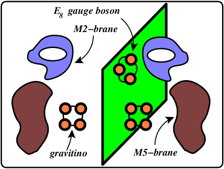
Figure 1: A typical state in heterotic M-theory. One gravitino and one gauge boson are depicted as bound states of D0-branes.

More complicated dynamics arise when we consider the formal ${\mathbb{Z}}_{2}$ orientifold of the BFSS model, namely the ${\mathrm{O}}(N)$ heterotic matrix model [10, 11, 12, 13, 14, 15, 16, 17]. In the ${\mathbb{Z}}_{2}$ quotient of M-theory in 11 dimensions, we find not only the gravity multiplet but also a gauge multiplet confined to the fixed locus of the ${\mathbb{Z}}_{2}$ orientifold, otherwise known as the Hořava-Witten domain wall [18, 19]. So there should be appropriate bound states in the quantum mechanics describing these states as well.

A separate line of reasoning [20] led to the discovery of a massive deformation of the BFSS matrix model. The deformed model describes M-theory on a plane wave background which arises as the Penrose limit of $AdS_{4}\times S^{7}$ or of $AdS_{7}\times S^{4}$ (they turn out to be identical). One major advantage of this model is that the usual difficulties in matrix theory associated with finding the bound state spectrum are absent; the mass deformation lifts all the flat directions and so the states corresponding to the graviton supermultiplet as well as the multi-graviton states are easy to find. In fact, they are localized near the “fuzzy sphere” classical configurations which are related to well-known giant gravitons [21]. In the limit of infinite background flux $\mu$, the action becomes quadratic and the theory can be solved perturbatively in $1/\mu$.

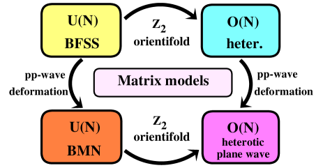
Figure 2: A commutative diagram showing the flat space BFSS Matrix theory, its ${\mathbb{Z}}_{2}$ orientifold, and their pp-wave massive deformations.

In this paper we combine the methods of heterotic matrix models with those of pp-wave matrix models by taking a ${\mathbb{Z}}_{2}$ quotient of the BMN matrix model. We will find that the massive deformation brings the same advantage here that it brought in the maximally supersymmetric case: namely, we will be able to see the vector supermultiplet carried by classical “giant gluons,” which are hemispherical membranes with fermionic degrees of freedom supported on the boundary.

The paper [22] also presented evidence that in the BMN matrix model a vacuum corresponding to a large number of very small spherical membranes admits a dual interpretation as a spherical transverse fivebrane—an object which had previously eluded detection in the matrix theory framework [23]. In our model we will find a corresponding fivebrane vacuum; it is a candidate to describe a spherical fivebrane immersed in the domain wall. We will give some evidence for this identification.

2 Brief review of the BMN matrix model

We begin with the maximally supersymmetric plane wave background of 11-dimensional supergravity, which can be obtained as a Penrose limit of $AdS_{4}\times S^{7}$ or of $AdS_{7}\times S^{4}$ [24]:

$$ds^{2} =-2dx^{+}dx^{-}+\sum_{A=1}^{9}dx^{A}dx^{A}-\left(\sum_{i=1}^{3}\left(\frac{\mu}{3}\right)^{2}x^{i}x^{i}+\sum_{a=4}^{9}\left(\frac{\mu}{6}\right)^{2}x^{a}x^{a}\right)dx^{+}dx^{+},$$ (1)

$$F_{123+} =\mu.$$ (2)

Berenstein, Maldacena, and Nastase [20] proposed a supersymmetric matrix model describing discrete light-cone quantization (DLCQ) of M-theory in the background (1). Its Hamiltonian can be thought of as a massive deformation of the BFSS matrix model [2]

$$H=H_{0}+H_{\mu}\equiv p^{-}.$$ (3)

Here $H_{0}$ is the BFSS Hamiltonian describing DLCQ of M-theory in 11 flat dimensions,

$$H_{0}=R\mathop{\rm Tr}\nolimits\left(\frac{1}{2}\Pi_{A}^{2}-\frac{1}{4}[X^{A},X^{B}]^{2}-\frac{1}{2}\Psi^{t}\gamma^{A}[X^{A},\Psi]\right)$$ (4)

and $H_{\mu}$ is the massive deformation

$$H_{\mu}=\frac{R}{2}\mathop{\rm Tr}\nolimits\left(\left(\frac{\mu}{3R}\right)^{2}(X^{i})^{2}+\left(\frac{\mu}{6R}\right)^{2}(X^{a})^{2}+i\frac{\mu}{4R}\Psi^{T}\gamma^{123}\Psi+i\frac{2\mu}{3R}\epsilon^{ijk}X^{i}X^{j}X^{k}\right).$$ (5)

Here $\Psi$ is a set of $16$ Grassmann-valued Hermitian matrices transforming as the $16$-component real spinor of $\mathop{\rm SO}\nolimits(9)$, $i$ runs from $1$ to $3$, $a$ runs from 4 to 9, and $A$ runs from $1$ to $9$.

This Hamiltonian has symmetry supergroup $\mathop{\rm SU}\nolimits(4|2)$ and it is convenient to write it in a way which makes that manifest. For the bosons we have done this already by splitting the indices into $i$ and $a$. For the fermions a convenient formalism appeared in [25]: under

$$\mathop{\rm SO}\nolimits(9) \to\mathop{\rm SO}\nolimits(6)\times\mathop{\rm SO}\nolimits(3)$$ (6)

the fermions split as

$$\bf{16} \to(\bf{4},\bf{2})\oplus(\bar{\bf{4}},\bf{2})$$ (7)

$$\Psi \to\psi_{I\alpha}\oplus\tilde{\psi}^{J\beta}$$ (8)

where $I$ is the fundamental index for $\mathop{\rm SU}\nolimits(4)$ and $\alpha$ is a 2-component spinor (fundamental) index for $\mathop{\rm SU}\nolimits(2)$. The reality condition on $\Psi$ implies that $\tilde{\psi}$ is not independent but rather can be written in terms of $\psi$, $(\psi^{\dagger})^{I\alpha}=\tilde{\psi}^{I\alpha}$. Then introducing the notation ${\tt{g}}^{a}_{IJ}$ for the Clebsch-Gordon coefficients $\bar{\bf{4}}\otimes\bar{\bf{4}}\to\bf{6}$, normalized so that

$${\tt{g}}^{a}({\tt{g}}^{b})^{\dagger}+{\tt{g}}^{b}({\tt{g}}^{a})^{\dagger}=2\delta^{ab},$$ (9)

we can rewrite the above Hamiltonian

$$H_{0} = R\mathop{\rm Tr}\nolimits\left(\frac{1}{2}\Pi_{A}^{2}-\frac{1}{4}[X^{A},X^{B}]^{2}+\psi^{\dagger I\alpha}\sigma^{i\beta}_{\alpha}[X^{i},\psi_{I\beta}]\right.$$ (10)

$$- \left.\frac{1}{2}\epsilon_{\alpha\beta}\psi^{\dagger\alpha I}{\tt{g}}^{a}_{IJ}[X^{a},\psi^{\dagger\beta J}]+\frac{1}{2}\epsilon^{\alpha\beta}\psi_{\alpha I}({\tt{g}}^{\dagger})^{aIJ}[X^{a},\psi_{\beta J}]\right),$$ (11)

$$H_{\mu} = \frac{R}{2}\mathop{\rm Tr}\nolimits\left(\left(\frac{\mu}{3R}\right)^{2}(X^{i})^{2}+\left(\frac{\mu}{6R}\right)^{2}(X^{a})^{2}+\frac{\mu}{2R}\psi^{\dagger I\alpha}\psi_{I\alpha}+i\frac{2\mu}{3R}\epsilon^{ijk}X^{i}X^{j}X^{k}\right).$$ (12)

For later use we also record the kinetic part of the Lagrangian,

$$\mathcal{L}_{kin}=\mathop{\rm Tr}\nolimits\left(\frac{1}{2R}(D_{0}X^{A})^{2}+i\Psi^{\dagger I\alpha}D_{0}\Psi_{I\alpha}\right),$$ (13)

which implies the equal time commutators

$$[(X^{A})_{mn},(\Pi_{B})_{kl}] =i\delta_{ml}\delta_{nk}\delta_{AB},$$ (14)

$$[(\psi_{I\alpha})_{mn},(\psi^{\dagger J\beta})_{kl}] =\delta_{ml}\delta_{nk}\delta^{\beta}_{\alpha}\delta^{I}_{J},$$ (15)

with

$$\Pi_{A}=\frac{1}{R}D_{0}X^{A}.$$ (16)

The lightlike decompactification limit, in which one expects to recover M-theory on the plane wave (1), is $N\to\infty$ with $p^{+}=N/R$ held fixed. Unlike in the BFSS model where only the states with energies of order $R/N$ survived the large $N$ limit (to keep $p^{+}p^{-}$ of order one in Planck units), here we should keep states whose energies are finite in units of $\mu$ as $N\to\infty$, so that $p^{+}p^{-}$ scales like the boost-invariant combination $\mu p^{+}$.

The BMN matrix model has several nice properties which were absent in the original BFSS model. For example, in the $\mu\to\infty$ limit the Hamiltonian becomes quadratic, which allows one to calculate physical observables in a perturbation expansion in powers of $R/\mu$ [25]. In fact, the representation theory of $\mathop{\rm SU}\nolimits(4|2)$ makes it possible to argue that some states have protected energies; in particular the energy remains finite as we move away from $\mu=\infty$ and these states therefore can be identified even at finite $\mu$ [26] (see also [27]). Also, the old puzzle of finding transverse fivebranes in matrix theory [23] seems to be more tractable once we include the mass deformation: transverse spherical fivebranes arise from strongly coupled dynamics in a vacuum containing a large number of coincident “small” membranes [22].

3 Orientifolding the BMN model

M-theory on the plane wave (1) possesses a ${\mathbb{Z}}_{2}$ symmetry which at the supergravity level is just $x^{3}\leftrightarrow-x^{3},C\leftrightarrow-C$. (We could also have chosen $x^{1}$ or $x^{2}$, but any other $x^{a}$ would not work because we would not obtain a symmetry of the field strength $F_{4}$.) So we can consider orientifolding this background and study M-theory on the resulting geometry. It is known from anomaly cancellation that in order to define $11$-dimensional supergravity on a manifold with boundary one has to introduce an extra $E_{8}$ gauge theory living only on the boundary [18, 19]. The same arguments apply in the presence of the plane wave deformation, so we expect that M-theory on our orientifolded plane wave will also contain an extra $E_{8}$ super Yang-Mills theory living at $X^{3}=0$. In the matrix model we will see this $E_{8}$ as a global symmetry of the $\mu\to\infty$, $N\to\infty$ spectrum.

By making the appropriate projection in the BMN matrix model, and adding extra fermionic degrees of freedom (0-8 strings) which reflect the coupling of the D0-branes to the gauge theory on the boundary—or, equivalently, are necessary to cancel the anomaly in the open membrane worldvolume theory [18]—we obtain a DLCQ description of M-theory on the orbifolded plane wave which is the Penrose limit of $AdS_{7}\times(S^{4}/{\mathbb{Z}}_{2})$ or $(AdS_{4})/{\mathbb{Z}}_{2}\times S^{7}$. The construction is very similar to previous work in the flat space case [10, 11, 12, 13, 14, 15, 16, 17]. We now describe it in more detail.

3.1 The ${\mathbb{Z}}_{2}$ projection

From now on we single out the index $3$, so $i=1,2$; $a=4,\dots,9$; and $A=1,2,4,5,6,7,8,9$. Then the BMN Hamiltonian (10), (12) has a ${\mathbb{Z}}_{2}$ symmetry,

$$X^{3} \to-(X^{3})^{T},$$ (17)

$$X^{A} \to+(X^{A})^{T},$$ (18)

$$\psi_{I\alpha} \to+(\sigma^{3})_{\alpha}^{\ \beta}(\psi_{I\beta})^{T}$$ (19)

where ^T refers to transposition of the $\mathop{\rm{}U}\nolimits(N)$ indices. (We could equally well have used $-\!\sigma^{3}$ instead of $+\!\sigma^{3}$ in (19) above; the choice amounts to a choice of chirality of the ten-dimensional $E_{8}$ gauge theory on the boundary.) Then we can truncate the fundamental fields to their ${\mathbb{Z}}_{2}$ invariant parts. For the bosons this gives a real antisymmetric matrix $\frac{i}{2}(X^{3}-(X^{3})^{T})$ and eight real symmetric matrices $\frac{1}{2}(X^{A}+(X^{A})^{T})$, which are denoted $A^{3}$ and $X^{A}$ respectively in the orientifold model. For the fermions, $\psi_{I\alpha}$ decomposes into $\psi_{I+}=\psi_{I1}$ and $\psi_{I-}=\psi_{I2}$ (the notation is meant to emphasize the $\sigma^{3}$ eigenvalue) and the projection (19) reduces these from Hermitian matrices to symmetric and antisymmetric matrices respectively. When there is no confusion we drop $I$, the $\mathop{\rm SU}\nolimits(4)$ index. The Hamiltonian for these fields can then be obtained just by truncation of (10) and (12); it is

$$H_{0}=R\mathop{\rm Tr}\nolimits\left[\frac{1}{2}\Pi_{A}^{2}-\frac{1}{2}E_{3}^{2}-\frac{1}{4}[X^{A},X^{B}]^{2}+\frac{1}{2}[A^{3},X^{A}]^{2}+i\psi_{+}^{\dagger I}[A^{3},\psi_{I+}]-i\psi_{a}^{\dagger I}[A^{3},\psi_{I-}]\right.\\ +\left.\psi_{+}^{\dagger I}[X^{1}-iX^{2},\psi_{I-}]+\psi_{-}^{\dagger I}[X^{1}+iX^{2},\psi_{I+}]+\left({\tt{g}}^{a}_{IJ}X^{a}\{\psi^{\dagger I}_{+},\psi^{\dagger J}_{-}\}+h.c.\right)\right]$$ (20)

and

$$H_{\mu} = \frac{R}{2}\mathop{\rm Tr}\nolimits\left[-\left(\frac{\mu}{3R}\right)^{2}(A^{3})^{2}+\left(\frac{\mu}{3R}\right)^{2}(X^{i})^{2}+\left(\frac{\mu}{6R}\right)^{2}(X^{a})^{2}\right.$$ (21)

$$- \left.\frac{2\mu}{R}A^{3}[X^{1},X^{2}]+\frac{\mu}{2R}(\psi^{\dagger I}_{+}\psi_{I+}+\psi^{\dagger I}_{-}\psi_{I-})\right],$$ (22)

where $E_{3}=\frac{1}{R}D_{0}A^{3}$. Similarly truncating the kinetic Lagrangian (13) gives

$$\mathcal{L}_{kin}=\mathop{\rm Tr}\nolimits\left[\frac{1}{2R}(D_{0}X^{A})^{2}-\frac{1}{2R}(D_{0}A^{3})^{2}+i\psi^{\dagger I}_{+}D_{0}\psi_{I+}+i\psi^{\dagger I}_{-}D_{0}\psi_{I-}\right]$$ (23)

which leads to the canonical commutation relations

$$[(X^{A})_{mn},(\Pi_{B})_{kl}] =\frac{i}{2}(\delta_{ml}\delta_{nk}+\delta_{mk}\delta_{nl})\delta_{AB},$$ (24)

$$[(A^{3})_{mn},(E_{3})_{kl}] =\frac{i}{2}(\delta_{ml}\delta_{nk}-\delta_{mk}\delta_{nl}),$$ (25)

$$\{(\psi_{I+})_{mn},(\psi^{\dagger J}_{+})_{kl}\} =\frac{1}{2}(\delta_{ml}\delta_{nk}+\delta_{mk}\delta_{nl})\delta_{I}^{J},$$ (26)

$$\{(\psi_{I-})_{mn},(\psi^{\dagger J}_{-})_{kl}\} =\frac{1}{2}(\delta_{ml}\delta_{nk}-\delta_{mk}\delta_{nl})\delta_{I}^{J}.$$ (27)

After the ${\mathbb{Z}}_{2}$ projection the gauge group of the matrix model is reduced to ${\mathrm{O}}(N)$ and the model describes the plane wave (1). We define

$$p^{+}=N/2R.$$ (28)

To see that this definition is appropriate in the M-theory limit, note that the physics of the ${\mathrm{O}}(2k)$ matrix model reduces via the Higgs mechanism to that of the $\mathop{\rm{}U}\nolimits(k)$ model far away from the domain wall, and (28) agrees with the known $p^{+}=k/R$ in this case. Another way of understanding this rule is that the total $p^{+}$ of an object in the original $\mathop{\rm{}U}\nolimits(N)$ model is now divided among two mirror images. In any case, the correspondence (28) implies that the states appearing in the ${\mathrm{O}}(N)$ matrix models with $N$ odd correspond to fields in spacetime which are antiperiodic around $x^{-}$. Such states appear because of a Wilson line around $x^{-}$, breaking the gauge group $E_{8}$ to $\mathop{\rm SO}\nolimits(16)$.

3.2 The symmetry superalgebra $\mathop{\rm SU}\nolimits(4|1)\times\mathop{\rm{}U}\nolimits(1)$

In Appendix B of [25] one can find the explicit operator realization of the superalgebra of the BMN matrix model in terms of matrices, together with all of the commutation relations. We now work out the ${\mathbb{Z}}_{2}$ projection of this superalgebra, which will be relevant for our model.

First we consider the fermionic generators. The BMN symmetry superalgebra is generated by 16 kinematical (nonlinearly realized) and 16 dynamical (linearly realized) supercharges, which in our $\mathop{\rm SO}\nolimits(3)\times\mathop{\rm SO}\nolimits(6)$ notation are denoted $q_{I\alpha}$ and $Q_{I\alpha}$ respectively. The $q_{I\alpha}$ involve only the $\mathop{\rm{}U}\nolimits(1)$ part of the $\mathop{\rm{}U}\nolimits(N)$ matrices:

$$q_{I\alpha}=\frac{1}{\sqrt{R}}\mathop{\rm Tr}\nolimits(\psi_{I\alpha}).$$ (29)

After the projection (19) $q_{I\alpha}$ is identified with $(\sigma^{3})_{\alpha}^{\beta}q_{I\beta}$, so the $q_{I-}$ component is projected out, leaving only $q_{I+}\equiv q_{I}$. Similarly,

$$Q_{I\alpha}= \sqrt{R}\mathop{\rm Tr}\nolimits\left[(\Pi^{a}-i\frac{\mu}{6R}X^{a}){\tt{g}}^{a}_{IJ}\epsilon_{\alpha\beta}\psi^{\dagger J\beta}-(\Pi^{i}+i\frac{\mu}{3R}X^{i})\sigma^{i\beta}_{\alpha}\psi_{I\beta}\right.$$ (30)

$$\left.+\frac{1}{2}[X^{i},X^{j}]\epsilon^{ijk}\sigma^{k\beta}_{\alpha}\psi_{I\beta}-\frac{i}{2}[X^{a},X^{b}]({\tt{g}}^{ab})^{J}_{I}\psi_{J\alpha}+i[X^{i},X^{a}]\sigma^{i}{\tt{g}}^{a}_{IJ}\epsilon_{\alpha\beta}\psi^{\dagger J\beta}\right],$$ (31)

and under the ${\mathbb{Z}}_{2}$ projection we see that $Q_{I+}$ is projected out; the only remaining component is $Q_{I-}\equiv Q_{I}$. Hence the heterotic plane wave matrix model has 16 real supercharges.

Next consider the bosonic generators. In the BMN model the $Q_{I\alpha}$ generate a simple superalgebra which was identified in [26, 29] as $\mathop{\rm SU}\nolimits(4|2)$. The bosonic generators of $\mathop{\rm SU}\nolimits(2)\times\mathop{\rm SU}\nolimits(4)\simeq\mathop{\rm SO}\nolimits(3)\times\mathop{\rm SO}\nolimits(6)$ are $M_{ij}$ and $M_{ab}$, given by

$$M_{ij} = \mathop{\rm Tr}\nolimits(X^{i}\Pi^{j}-X^{j}\Pi^{i}+\frac{1}{2}\epsilon^{ijk}\psi^{\dagger}\sigma^{k}\psi)\ ,$$ (32)

$$M_{ab} = \mathop{\rm Tr}\nolimits(X^{a}\Pi^{b}-X^{b}\Pi^{a}+\frac{1}{2}\psi^{\dagger}{\tt{g}}^{ab}\psi).$$ (33)

Under the ${\mathbb{Z}}_{2}$ action $M_{13}$ and $M_{23}$ have eigenvalue $-1$, so they are not symmetries of the reduced theory, whereas $M^{12}$ and $M_{ab}$ survive the projection.

We also have the bosonic generators $a_{a},a_{i}$ in the $\mathop{\rm{}U}\nolimits(1)$ sector of the BMN model, which appear in the anticommutator of the $q_{I\alpha}$:

$$a_{i} =\frac{1}{\sqrt{R}}\mathop{\rm Tr}\nolimits\left(\sqrt{\frac{\mu}{6R}}X^{i}+\sqrt{\frac{3R}{2\mu}}i\Pi^{i}\right),$$ (34)

$$a_{a} =\frac{1}{\sqrt{R}}\mathop{\rm Tr}\nolimits\left(\sqrt{\frac{\mu}{12R}}X^{a}+\sqrt{\frac{3R}{\mu}}i\Pi^{a}\right).$$ (35)

Under the ${\mathbb{Z}}_{2}$ projection all of these operators survive except for $a_{3}$, which is projected out.

Having catalogued the surviving symmetry generators we can now write out their algebra, which is the ${\mathbb{Z}}_{2}$ projection of that given in [25]. The important anticommutators are

$$\{Q^{\dagger I},Q_{J}\} = 2\delta^{I}_{J}H-\frac{i\mu}{6}({\tt{g}}^{ab})^{I}_{\ J}M^{ab}+\frac{2\mu}{3}\delta^{I}_{J}M^{12}\$$ (36)

$$= 2\delta^{I}_{J}{\cal H}-\frac{i\mu}{6}({\tt{g}}^{ab})^{I}_{\ J}M^{ab},$$ (37)

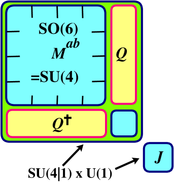
Figure 3: The structure of $\mathop{\rm SU}\nolimits(4|1)\times\mathop{\rm{}U}\nolimits(1)$. ${\cal H}$, not shown, is a diagonal matrix of $\mathop{\rm SU}\nolimits(4|1)$, chosen so that its supertrace vanishes.

where we have defined

$${\cal H}=H+\frac{\mu}{3}M^{12},$$ (38)

and

$$[{\cal H},q_{I}] = -\frac{5\mu}{12}q_{I}\$$ (39)

$$[{\cal H},Q_{I}] = +\frac{\mu}{4}Q_{I}.$$ (40)

In sum, the bosonic part of the symmetry supergroup in the orientifolded theory is $\mathop{\rm SU}\nolimits(4)\times\mathop{\rm{}U}\nolimits(1)\times\mathop{\rm{}U}\nolimits(1)$, where the two $\mathop{\rm{}U}\nolimits(1)$ factors are generated by $H$ and $M^{12}$. However, only one combination of the two $\mathop{\rm{}U}\nolimits(1)$’s occurs in the anticommutator of the supercharges; we have denoted the generator of this $\mathop{\rm{}U}\nolimits(1)$ by ${\cal H}$. This $\mathop{\rm{}U}\nolimits(1)$ combines with $\mathop{\rm SU}\nolimits(4)$ and the dynamical supercharges $Q_{I},Q^{I\dagger}$ to give the simple supergroup $\mathop{\rm SU}\nolimits(4|1)$. However, there is another combination of the $\mathop{\rm{}U}\nolimits(1)$’s, so the full symmetry is $\mathop{\rm SU}\nolimits(4|1)\times\mathop{\rm{}U}\nolimits(1)$. The generator of the other $\mathop{\rm{}U}\nolimits(1)$, $J$, must commute with $\mathop{\rm SU}\nolimits(4|1)$, so in particular it commutes with $Q_{I}$. This requirement implies that we should choose

$$J\,=\,H\!-\!\frac{\mu}{6}M^{12}\,=\,{\cal H}\!-\!\frac{\mu}{2}M^{12}\,=\,\frac{1}{2}(3H\!-\!{\cal H}),$$ (41)

which satisfies

$$[J,Q_{I}]=0,\ \ \ [J,{\cal H}]=0,$$ (42)

and furthermore

$$[J,q_{I}]=-\frac{\mu}{6}q_{I}.$$ (43)

So far we have only discussed the superalgebra which acts on gauge invariant (uncharged) states. More generally we could consider arbitrary states, and in this case the commutator (36) of the supercharges is modified by the addition of a gauge charge on the right side:

$$\{Q^{\dagger I},Q_{J}\}=2\delta^{I}_{J}({\cal H}+A^{3}_{mn}G_{mn})-\frac{i\mu}{6}({\tt{g}}^{ab})^{I}_{\ J}M^{ab}$$ (44)

Here $G_{mn}$ represents the charge under the $\mathop{\rm SO}\nolimits(N)$ generator $E_{mn}$ which is an antisymmetric matrix:

$$(E_{mn})_{ij}=\delta_{mi}\delta_{nj}-\delta_{ni}\delta_{mj}.$$ (45)

The generator $G_{mn}$ can be explicitly written in terms of the fields as

$$G_{mn} = \frac{1}{2}\left(E^{3}_{mk}A^{3}_{kn}-A^{3}_{mk}E^{3}_{kn}\right)-\frac{1}{2}\sum_{A}\left(X^{A}_{mk}\Pi^{A}_{kn}-\Pi^{A}_{mk}X^{A}_{kn}\right)+$$ (46)

$$+ \sum_{I=1}^{4}\left(\psi_{I+,k[m}\psi^{I\dagger}_{+,n]k}+\psi_{I-,k[m}\psi^{I\dagger}_{-,n]k}\right)+i\sum_{r=1}^{16}\lambda^{r}_{[m}\lambda^{r}_{n]}.$$ (47)

Note the $\lambda$ part of $G_{mn}$ which is important and will be discussed in the following subsection.

3.3 The $\lambda$ fields

The field content of the orientifold model is not just the ${\mathbb{Z}}_{2}$ projection of the BMN model; we must add 16 real fermions $\lambda^{r}$ ($r=1,\dots,16$) in the fundamental representation of ${\mathrm{O}}(N)$. This is precisely analogous to what happens in the flat space heterotic matrix models [10, 13]. In that case one can understand the need for $16$ fermions in two ways: if we think of the heterotic matrix model as describing D0-branes in Type I’, then the $\lambda^{r}$ arise from quantization of the 0-8 strings; on the other hand, if we think of the heterotic matrix model as the ${\mathbb{Z}}_{2}$ quotient of the BFSS matrix model, we find a linear potential for $X$ which destroys translation invariance even far from the domain wall unless we add the $\lambda^{r}$ [13]. When we study the spectrum of our model we will find a similar mechanism which fixes the number of $\lambda^{r}$ to be $16$ in our case as well; namely, this number is essential to ensure finiteness of the quantum numbers of the fuzzy hemispherical membrane’s ground state.

Let us consider how the addition of the $\lambda$ fields modifies the superalgebra discussed above. Since the $\lambda^{r}$ are charged under ${\mathrm{O}}(N)$, the Lagrangian in the orientifold matrix model contains a covariant kinetic term

$$\mathcal{L}_{kin,\lambda}=i(\lambda^{r})^{T}D_{0}\lambda^{r}.$$ (48)

However, this cannot be the only term involving $\lambda$, because $A^{0}$ transforms nontrivially under the ${\mathbb{Z}}_{2}$ projected supersymmetry algebra [2]. This transformation can be compensated by fixing the full $\lambda$ dependent part of the Lagrangian to be

$$\mathcal{L}_{\lambda}=i(\lambda^{r})^{T}(D_{0}-A^{3})\lambda^{r}.$$ (49)

Then since $A^{0}$ and $A^{3}$ have the same variation under the surviving 16 supersymmetries, the full action will be supersymmetric provided we take the $\lambda^{r}$ to be invariant [13].

From (49) we find the $\lambda$ dependent part of the Hamiltonian (in the gauge $A^{0}=0$):

$$H_{\lambda}=i(\lambda^{r})^{T}A^{3}\lambda^{r}.$$ (50)

The full Hamiltonian is

$$H=H_{0}+H_{\mu}+H_{\lambda}$$ (51)

with the three pieces given in (20), (21), (50).

The fact that $H$ depends on the $\lambda^{r}$ creates a puzzle, since the $\lambda^{r}$ do not appear in the $Q_{I}$ — how can this be consistent with the commutator (36)? This puzzle is resolved (as in the flat space case [13]) by recalling that the question of whether $\lambda^{r}$ appear or not in a given generator is not meaningful if we only consider the algebra acting on gauge invariant states, because in that case we are always free to add gauge charges to the generators. If we consider the full commutator (44) acting on arbitrary states, the $\lambda$ dependence indeed vanishes on both sides: since each $\lambda^{r}$ is a vector of ${\mathrm{O}}(N)$, the gauge charge $A^{3}G$ includes $(\lambda^{r})^{T}A^{3}\lambda^{r}$, which cancels $H_{\lambda}$ (50). Everything is therefore consistent provided that there is no $\lambda$ dependence in $M^{12}$, so the $\lambda^{r}$ are uncharged under this spatial rotation. (However, in certain classical vacua the $\lambda^{r}$ acquire an effective $M^{12}$—see Section 6.1.)

In sum, the generators of $\mathop{\rm SU}\nolimits(4|1)\times\mathop{\rm{}U}\nolimits(1)_{J}$ are given by the naive ${\mathbb{Z}}_{2}$ projections of their $\mathop{\rm SU}\nolimits(4|2)$ counterparts, with the exception that $H$ must be modified to include $H_{\lambda}$ given in (50).

4 Classical vacua: open fuzzy membranes

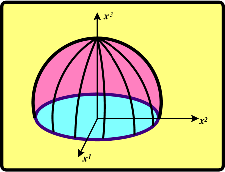
Figure 4: Hemispherical M2-brane ending on a Hořava-Witten domain wall $x^{3}=0$.

Any classical solution of the original $\mathop{\rm{}U}\nolimits(N)$ BMN model can be described in terms of a (generally reducible) $N$-dimensional representation of $\mathop{\rm SU}\nolimits(2)$. Namely, the three adjoint scalar matrices $X^{i}$ are the only variables that acquire nonzero vacuum expectation values, given by [20, 25]:

$$X^{i}=\frac{\mu}{3R}J^{i},\quad i=1,2,3$$ (52)

where the $c$-number matrices $J^{i}$ satisfy the standard $\mathop{\rm SU}\nolimits(2)$ commutation relations. Each such representation can be decomposed into irreducible representations of $\mathop{\rm SU}\nolimits(2)$. Then the $X^{i}$ are block-diagonal and each block, i.e. each irreducible representation of $\mathop{\rm SU}\nolimits(2)$, is interpreted as a fuzzy spherical membrane. Up to gauge equivalence the solution is uniquely specified by the dimensions $N_{k}$ of the irreducible representations, subject to

$$\sum_{k=1}^{n}N_{k}=N.$$ (53)

We denote the solution by $(N_{1},N_{2},\dots,N_{n})$. The $N_{k}$ are related to the physical radii of the $n$ fuzzy spheres. For simplicity, consider the irreducible case; then the eigenvalues of each $J^{i}$ belong to the set $\{-j,-j+1,\dots,j-1,j\}$ with $j=(N-1)/2$, so the physical radius is

$$R_{M2}=\frac{\mu}{3R}\sqrt{j(j+1)}=\frac{\mu}{6R}\sqrt{N^{2}-1}.$$ (54)

Next we want to see whether these classical solutions of the BMN model give rise to classical solutions of our orientifold model. Any classical solution of the original model that satisfies the ${\mathbb{Z}}_{2}$ constraints (17)-(19) becomes a solution of our theory automatically: if the action is stationary with respect to any variations, it is of course also stationary with respect to the ${\mathbb{Z}}_{2}$ invariant variations. Note that in any representation of $\mathop{\rm SU}\nolimits(2)$ there is a standard basis for which two generators are symmetric while one is antisymmetric. Our convention (which agrees with the one adopted in [25]) is that $J^{3}$ is antisymmetric while $J^{1},J^{2}$ are symmetric. Hence we can identify the antisymmetric generator with $A^{3}$ while the symmetric ones are $X^{1},X^{2}$. Therefore every solution of the original BMN model induces a solution of our orientifold model.

Since our model describes a space in which $x^{3}$ has been identified with $-x^{3}$, these solutions are naturally interpreted in our model as collections of hemispherical membranes rather than spherical ones. This makes sense since it has been known since the early days of matrix theory [11, 12] that, for large $N$, ${\mathrm{O}}(N)$ can approximate the group of area-preserving diffeomorphisms of the disk, similar to the way $\mathop{\rm{}U}\nolimits(N)$ approximates the group of area-preserving diffeomorphisms of a closed oriented membrane [3].

In summary, the ${\mathrm{O}}(N)$ plane wave matrix model inherits the classical solutions of its $\mathop{\rm{}U}\nolimits(N)$ predecessor; these are described by $N$-dimensional representations of $\mathop{\rm SU}\nolimits(2)$, and are interpreted as collections of concentric hemispherical membranes, with radii fixed by the dimension of the irreducible subrepresentations as in (54).

5 Representations of $\mathop{\rm SU}\nolimits(4|1)$

As explained in Section 3.2, the symmetry algebra of the heterotic BMN matrix model is $\mathop{\rm SU}\nolimits(4|1)\times\mathop{\rm{}U}\nolimits(1)_{J}\times G$ (where $G$ is the global symmetry which acts on the $\lambda$ fields; $G$ manifestly includes $\mathop{\rm SO}\nolimits(16)$ and we will eventually see that it is enhanced to $E_{8}$ in the large $N$ limit at least in some vacua.) In this section we will focus on the $\mathop{\rm SU}\nolimits(4|1)$ superalgebra and study its unitary irreducible representations. Our discussion in this section is essentially a review of the work by Kac [30] and Bars et al. [31, 32], specialized to the case of $\mathop{\rm SU}\nolimits(4|1)$. A closely analogous and significantly more detailed discussion in the $\mathop{\rm SU}\nolimits(4|2)$ case may be found in [26, 29].

Any representation of $\mathop{\rm SU}\nolimits(4|1)$ may be decomposed under $\mathop{\rm SU}\nolimits(4)$ into a set of irreducible representations, each labelled by the eigenvalue of ${\cal H}$. Starting with states $|\psi\rangle$ which form some representation of $\mathop{\rm SU}\nolimits(4)$, the other fermionic and bosonic states in the same supermultiplet can be obtained by acting with the supercharges $Q^{\dagger}_{I}$ or $Q_{I}$, $I=1,2,3,4$. Explicitly, a complete basis for the representation of $\mathop{\rm SU}\nolimits(4|1)$ is given by

$$(Q^{\dagger}_{1})^{{\bar{s}}_{1}}\ (Q^{\dagger}_{2})^{{\bar{s}}_{2}}\ (Q^{\dagger}_{3})^{{\bar{s}}_{3}}\ (Q^{\dagger}_{4})^{{\bar{s}}_{4}}(Q_{1})^{s_{1}}\ (Q_{2})^{s_{2}}\ (Q_{3})^{s_{3}}\ (Q_{4})^{s_{4}}|\psi\rangle$$ (55)

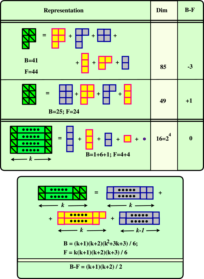
Figure 21: Some more examples of the simplest $\mathop{\rm SU}\nolimits(4|1)$ superdiagrams.

with ${\bar{s}}_{i},s_{i}=0,1$. (Note that since $\{Q_{I},Q_{J}\}=0$, this representation of $\mathop{\rm SU}\nolimits(4|1)$ is finite-dimensional, provided that the original representation of $\mathop{\rm SU}\nolimits(4)$ was finite-dimensional.) The simplest examples of representations of $\mathop{\rm SU}\nolimits(4|1)$ and their decomposition under $\mathop{\rm SU}\nolimits(4)$ are summarized in Figures 20, 21 at the end of this paper.

Just as for the ordinary Lie group $\mathop{\rm SU}\nolimits(n)$, there are two standard ways of constructing representations of $\mathop{\rm SU}\nolimits(4|1)$: the Kac-Dynkin method and the method of superdiagrams. We now describe these two in turn.

5.1 Kac-Dynkin method, typical and atypical representations

As discussed by Kac [30] (and reviewed in [26, 29]) the representation theory of simple Lie superalgebras parallels that of simple Lie algebras. One begins by finding a maximal set of commuting bosonic generators of the superalgebra; in our case such a set is $\{H_{i}\},\ i=1,2,3$, and these generators span a Cartan subalgebra of $\mathop{\rm SU}\nolimits(4)$. Then the remaining generators, bosonic and fermionic, can be chosen to be eigenvectors of $H_{i}$; the eigenvalues are called roots. In the $\mathop{\rm SU}\nolimits(4|1)$ case, only four of the positive roots are linearly independent; three are simple positive roots of $\mathop{\rm SU}\nolimits(4)$ and the last is fermionic. The positive roots and the Cartan algebra generators form a maximal subalgebra. In the Dynkin basis the positive and negative roots, $E_{i}$ and $F_{i}$, can be chosen such that

$$[H_{i},H_{j}]=0,\ \ [H_{i},E_{j}]=\alpha_{ij}E_{j},\ \ [H_{i},F_{j}]=-\alpha_{ij}F_{j},\ \ [E_{i},F_{j}]=\delta_{ij}H_{i}$$ (56)

and $\alpha_{ij}$, the Cartan matrix, is

Figure 5: Kac-Dynkin diagram of $\mathop{\rm SU}\nolimits(4|1)$.

$$\alpha=\left(\begin{array}[]{rrrr}2&-1&&\\ -1&2&-1&\\ &-1&2&-1\\ &&-1&0\end{array}\right).$$ (57)

This information may be summarized in a Kac-Dynkin diagram with four nodes, where the fourth node is fermionic and there are $|\alpha_{ij}\alpha_{ji}|$ lines joining the $i^{\mathrm{th}}$ and $j^{\mathrm{th}}$ nodes; see figure 5. One can then use this basis to construct finite dimensional representations as one does in the case of ordinary Lie groups. Each representation is uniquely determined by a weight vector $\Lambda$, known as the “highest weight”: by definition the representation is generated by a single state $|\Lambda\rangle$ with weight $\Lambda$ which is annihilated by all the positive roots. In the Kac-Dynkin basis we write

$$\Lambda=(a_{1},a_{2},a_{3}|a_{4}),$$ (58)

where $(a_{1},a_{2},a_{3})$ are $\mathop{\rm SU}\nolimits(4)$ Dynkin labels and hence are non-negative integers, while $a_{4}$ can be any real number. The eigenvalue of ${\cal H}$, the generator of the diagonal $\mathop{\rm{}U}\nolimits(1)\subset\mathop{\rm SU}\nolimits(4|1)$, for this state is

$${\cal H}_{0}=\mu\left(\frac{1}{12}a_{1}+\frac{1}{6}a_{2}+\frac{3}{4}a_{3}+a_{4}\right).$$ (59)

The other states in the multiplet can be obtained by the action of the $Q_{I}$’s on the highest weight state:

$$(Q_{1})^{s_{1}}\ (Q_{2})^{s_{2}}\ (Q_{3})^{s_{3}}\ (Q_{4})^{s_{4}}|\Lambda\rangle$$ (60)

where $s_{i}=0,1$. Note that in principle the multiplet generated in this way may be reducible. As argued in [30] all the unitary representations should have positive ${\cal H}$ and unitarizable representations should satisfy

$$a_{4}\geq 0.$$ (61)

In general, ${\cal{H}}\$for a state of the form (60) equals ${\cal H}_{0}+\frac{\mu}{4}\sum_{i}s_{i}$. Therefore, we can have at most five different ${\cal{H}}\$levels in the same multiplet, spaced by $\frac{\mu}{4}$.

If a representation includes all these five different ${\cal{H}}\$levels it is called typical. For unitary typical representations $a_{4}>0$ and hence ${\cal H}_{0}>\mu(\frac{1}{12}a_{1}+\frac{1}{6}a_{2}+\frac{3}{4}a_{3})$. The dimension of a typical representation $V(\Lambda)$ is simply given in terms of the dimension of the $\mathop{\rm SU}\nolimits(4)$ representation generated by the highest weight state:

$$\!\!\!\!\!\!\!\!\!\dim(V(\Lambda)) = 2^{4}\dim(V_{0}(\Lambda))$$ (62)

$$= \frac{2^{4}}{12}(a_{1}\!+\!1)(a_{2}\!+\!1)(a_{3}\!+\!1)(a_{1}\!+\!a_{2}\!+\!2)(a_{2}\!+\!a_{3}\!+\!2)(a_{1}\!+\!a_{2}\!+\!a_{3}\!+\!3).$$ (63)

However, it may happen that an irreducible representation includes fewer than five ${\cal{H}}\$levels; in this case the representation is called atypical. As was discussed in [30, 32], for atypical representations we must have

$$a_{4}\in\{-\!a_{3}\!-\!1,\,\,-\!a_{3}\!-\!a_{2}\!-\!2,\,\,-\!a_{3}\!-\!a_{2}\!-\!a_{1}\!-\!1,\,\,0\},$$ (64)

and therefore for the unitary atypical representations $a_{4}$ must vanish. As a result, the value of ${\cal H}_{0}$ in an atypical representation is already determined by the $\mathop{\rm SU}\nolimits(4)$ quantum numbers. In this way atypical representations are similar to BPS states; in contrast to the typical representations, which sit in continuous families parameterized by $a_{4}$, an atypical representation is rigid and has no continuous deformations. The dimension of an atypical representation is generally smaller than $2^{4}\dim(V_{0}(\Lambda))$. We will discuss the precise relation to BPS states in Section 5.3.

5.2 Young superdiagrams

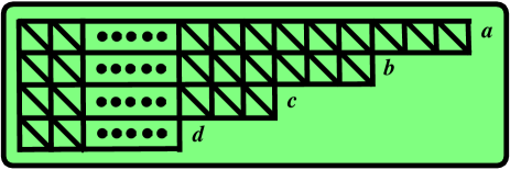
Figure 6: The most generic $\mathop{\rm SU}\nolimits(4|1)$ superdiagram.

In ordinary Lie algebras all finite dimensional representations can be obtained through (tensor) products of finitely many basic irreps. However, due to the existence of the continuous parameter $a_{4}$, this is not true for Lie superalgebras. Nevertheless, as we will see in the next sections, all the states in the spectrum of the orientifold of the BMN matrix model at $\mu=\infty$ do fit into tensor representations. Furthermore, as shown in [31, 32], for the $\mathop{\rm SU}\nolimits(m|n)$ case these tensor representations can be represented by a supersymmetric version of the standard Young diagrams. Here we review, very briefly, some basic facts about superdiagrams of $\mathop{\rm SU}\nolimits(4|1)$; for a more detailed discussion the reader is referred to [31, 32].

To a multiplet with highest weight $\Lambda=(a-b,b-c,c-d|d)$, where $d$ is a non-negative integer, we associate the superdiagram depicted in Figure 6. The value of ${\cal{H}}\$for the highest weight state is simply given by the total number of boxes:

$${\cal H}_{0}=\frac{\mu}{12}(a+b+c+d).$$ (65)

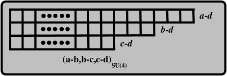
Figure 7: The $\mathop{\rm SU}\nolimits(4)$ representation in which both the states with the highest ${\cal H}$ states and those with the lowest ${\cal H}$ in the typical multiplet $(a-b,b-c,c-d|d)$ transform.

The other states in the superdiagram are obtained by acting on the highest weight state (with $\mathop{\rm SU}\nolimits(4)$ highest weight $(a-b,b-c,c-d)$) with the supercharges $Q_{I}$, which are in the $(1,0,0)$ representation of $\mathop{\rm SU}\nolimits(4)$.

Since we have only four different $Q_{I}$’s, if $d\neq 0$, the state obtained by acting with all of the $Q$’s on the highest weight state has the highest ${\cal{H}}\$eigenvalue in the multiplet, namely ${\cal H}=\frac{\mu}{12}(a+b+c+d)+\mu$. This state generates a $\mathop{\rm SU}\nolimits(4)$ representation isomorphic to that generated by the highest weight state itself; this representation is shown in Figure 7.

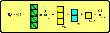
Figure 8: Expansion of the superdiagram corresponding to $(0,0,0|1)$ in terms of $\mathop{\rm SU}\nolimits(4)$ Young diagrams. The indices show the value of ${\cal{H}}\$(in units of $\mu$) for each state.

To illustrate the expansion of the superdiagram in terms of bosonic and fermionic modes, as an example we have worked out expansion of the representation with highest weight $(0,0,0|1)$ in Figure 8.

The typical and atypical representations can be easily identified in terms of superdiagrams: the superdiagrams with four rows ($d\neq 0$) are typical and those with less than four rows ($d=0$) are atypical.

Here we summarize some facts about $\mathop{\rm SU}\nolimits(4|1)$ superdiagrams:

• i) Superdiagrams of $\mathop{\rm SU}\nolimits(4|1)$ can at most have four rows.

• ii) The number of ${\cal H}$ levels in the representation (with steps of $\frac{\mu}{4}$) is the number of rows plus one.

• iii) For atypical representations the value of ${\cal{H}}\$for the highest weight state, and hence for all the other states in the multiplet, is completely determined by the $\mathop{\rm SU}\nolimits(4)$ quantum numbers.

• iv) The dimension of a typical representation is $2^{4}$ times the dimension of the $\mathop{\rm SU}\nolimits(4)$ representation generated from its highest weight state. The dimension of an atypical representation with highest weight $\Phi=(a-b,b-c,c|0)$ is

  $$\!\!\!\!\!\!\!\!\!\!\!\!\dim(V(\Phi))=\frac{2^{4}}{12} (a-b+1)(b-c+1)(a-c+2)\Bigg{[}\frac{1}{8}(-)^{c}[2(a-c+2)(b-c+1)-1]+$$ (67)

  $$\ \ \ \ +\sum_{l=1}^{c}(-)^{l+1}(a+3-l)(b+2-l)(c+1-l)\Bigg{]}.$$

• v) In our conventions the highest weight state of a superdiagram with an even (odd) number of boxes is bosonic (fermionic), in agreement with the spin-statistics relation for $M^{12}$.

• vi) Typical representations contain equal number of bosonic and fermionic states, while for atypical ones $B-F\neq 0$. In particular, for the representation with highest weight $(a-b,b-c,c|0)$,

  $$B-F=(-)^{a+b+c}\ \frac{1}{2}(a-b+1)(a-c+2)(b-c+1).$$ (68)

  So $B>F$ for atypical superdiagrams with an even number of boxes, and $B<F$ for atypicals with an odd number of boxes.

• vii) For any multiplet ${\cal X}$,

  $$\mathop{\mathrm{Str}}_{{\cal X}}({\cal H})\equiv\sum_{{\cal X}}(-)^{F}{\cal H}=0.$$ (69)

• viii) As stated above, we must have $a_{4}\geq 0$ for a representation to be unitary, and $a_{4}=0$ for atypical representations. If we take a typical representation $(a-b,b-c,c|d)$ and let $d\to 0$, however, we do not simply get the atypical representation $(a-b,b-c,c|0)$ but rather the direct sum of two atypicals, $(a-b,b-c,c|0)$ and $(a-b,b-c,c+1|0)$. Put another way, two atypical representations which are of the form $(a-b,b-c,c|0)$ and $(a-b,b-c,c+1|0)$ can combine into the typical representation $(a-b,b-c,c|\epsilon)$. The typical representation is created near $\epsilon=0$, but once it has been created the value of $\epsilon>0$—hence also of $\mathcal{H}$—can change continuously while the $\mathop{\rm SU}\nolimits(4)$ content is unchanged. For example, the typical tensor representation shown in Figure 9 has $\epsilon=1$.

• ix) The value of ${\cal{H}}\$in any state of an atypical representation is fixed by the representation’s $\mathop{\rm SU}\nolimits(4)$ content, and hence cannot receive corrections unless there exist other atypical representations which can combine with it to form a typical representation as described above.

  

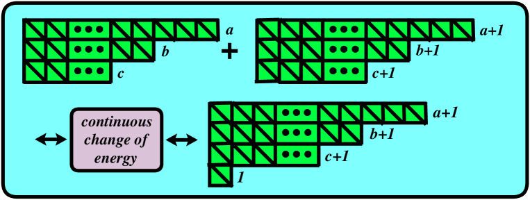
  Figure 9: Two atypical representations which can combine into the typical representation with highest weight $(a-b,b-c,c|\epsilon)$ whose $\mathop{\rm SU}\nolimits(4)$ content is identical to that of the tensor representation with heighest weight $(a-b,b-c,c|1)$ shown in the figure but whose values of ${\cal H}$ can change continuously.

• x) Any atypical representation $(a-b,b-c,c|0)$ can be extended to a chain of atypical representations, in which any representation can combine with either of its two neighbors into a typical representation. This chain necessarily terminates from one end at $(a-b,b-c,0|0)$. Unlike the $\mathop{\rm SU}\nolimits(4|2)$ case discussed in [26, 29], in the $\mathop{\rm SU}\nolimits(4|1)$ case the chain contains infinitely many diagrams ($c$ can be arbitrarily large).

5.3 BPS states and atypical representations

As we have discussed, states in atypical representations share some properties with the usual BPS states; for example, the values of ${\cal H}$ in such a multiplet are completely determined by the $\mathop{\rm SU}\nolimits(4)$ quantum numbers. One may wonder if these states are also BPS in the usual sense. Following [25, 26], let us check directly whether any of the states in an atypical superdiagram is killed by the right-hand-side of the superalgebra (36). First we rewrite the $({\tt{g}}^{ab})^{I}_{\ J}M^{ab}$ term in the superalgebra in terms of three $\mathop{\rm{}U}\nolimits(1)$ generators in the Cartan subalgebra of $\mathop{\rm SU}\nolimits(4)$; then

$$\!\!\!\!\!\!\!\langle\psi|\{Q_{I},Q^{\dagger J}\}|\psi\rangle \equiv \Delta_{\psi}\delta_{I}^{J}$$ (70)

$$= 2\left({\cal H}_{\psi}+\frac{\mu}{6}[s_{1}(I)M^{45}+s_{2}(I)M^{67}-s_{1}(I)s_{2}(I)M^{89}]\right)\delta_{I}^{J},$$ (71)

where $s_{i}(I)=\pm 1$ are independent functions of the index $I$, $M^{45},M^{67},M^{89}$ are the eigenvalues of the Cartan generators, and ${\cal H}_{\psi}$ is the eigenvalue of ${\cal{H}}\$for the highest weight state in the multiplet. In terms of a Dynkin basis [26, 29],

$$M^{45}=\frac{1}{2}(H_{1}+2H_{2}+H_{3}),\ \ M^{67}=\frac{1}{2}(H_{1}+H_{3}),\ \ M^{89}=\frac{1}{2}(H_{3}-H_{1}).$$ (72)

The number of supercharges preserved by the state $|\psi\rangle$ is twice the number of choices of $s_{i}$’s for which $\Delta_{\psi}$ vanishes.

First consider a singlet of $\mathop{\rm SU}\nolimits(4|1)$, for which all $M^{ab}$ as well as ${\cal H}$ vanish. Then there are four choices of $s_{1},s_{2}$ for which $\Delta$ vanishes, i.e. the vacua preserve all 8 dynamical supercharges. Hence they are $\frac{1}{2}$ BPS. (In the matrix model the vacua will be singlets of $\mathop{\rm SU}\nolimits(4|1)$, but they are not the only singlets. Note, however, that in the matrix model we also have $\mathop{\rm{}U}\nolimits(1)_{J}$, and $J=0$ for the vacua while $J>0$ for generic singlets.)

Next let us consider superdiagrams with only one row. It is straightforward to show that in this case $\Delta_{\psi}=0$ precisely when

$$s_{1}+s_{2}+s_{1}s_{2}=-1.$$ (73)

In fact this equation is satisfied with three (out of four) choices for the $s_{i}$’s, and so the highest weight  states of representations corresponding to one-row superdiagrams are $\frac{3}{8}$ BPS.

As for the superdiagrams with two rows, one can show that in this case $\Delta_{\psi}=0$ if and only if $s_{1}=-1$, so the highest weight state of these superdiagrams is $\frac{1}{4}$ BPS. For the diagrams with three rows, $\Delta_{\psi}=0$ only if $s_{1}=s_{2}=-1$; hence the highest weight state of such multiplets is $\frac{1}{8}$ BPS. The diagrams with four rows are typical representations and do not preserve any supercharges.

In summary, the highest weight state of a representation corresponding to a superdiagram with $r$ rows is $\frac{1}{8}(4-r)$ BPS (preserves $2\cdot(4-r)$ supercharges). We would like to point that this statement applies only to the highest weight state of the representation. Generically, the other states in the same multiplet (which have a higher ${\cal H}$) do not preserve any supercharges.

5.4 A supersymmetric index

To discuss nonperturbative properties of the spectrum it is useful to define an index, similar to [33], which is independent of the coupling $R/\mu$ (at least provided that no states contributing to the index become non-normalizable as we vary $\mu$.) Since we know the full spectrum of the theory at weak coupling ($\mu=\infty$) we can evaluate the index and in this way potentially extract some information about the non-perturbative spectrum of the matrix model. Our arguments parallel those of Appendix A of [22].

Among the four (complex) dynamical supercharges we single out one, $Q^{\dagger}$, which carries charge $\frac{1}{2}$ under three $\mathop{\rm{}U}\nolimits(1)$ factors of $\mathop{\rm SU}\nolimits(4)$:

$$[M^{45},Q^{\dagger}]=[M^{67},Q^{\dagger}]=[M^{89},Q^{\dagger}]=+\frac{1}{2}Q^{\dagger}.$$ (74)

Then $Q^{\dagger}$ satisfies

$$\{Q,Q^{\dagger}\}={\cal H}-\frac{\mu}{6}(M^{45}+M^{67}+M^{89})\equiv{\cal E}$$ (75)

From (39), (42) and (74), it is easy to show that

$$[Q,{\cal E}]=0,\ \ [J,{\cal E}]=0.$$ (76)

Furthermore, from (75) we see that the eigenvalues of ${\cal E}$ are all non-negative.

Now we define an index by

$${\cal I}=\mathrm{Str}(e^{-\beta{\cal E}}).$$ (77)

This index receives contributions only from states with ${\cal E}=0$ (which are necessarily annihilated by $Q$, hence BPS.) As usual for an index, ${\cal I}$ gives a lower bound on the number of states with ${\cal E}=0$. This bound is actually saturated if among the BPS multiplets which contribute there are none which can combine into typical (non-BPS) multiplets. We will see in section 8 that in some physically relevant cases we can indeed show that this bound is saturated.

At first ${\cal I}$ might seem like a rather crude invariant, since all atypical representations contain BPS states for which ${\cal E}=0$. However, there are some other operators which commute with the supercharges, so we can restrict ${\cal I}$ to their eigenspaces and get finer information. In section 3, we found one such label, $J$. Another label which will be convenient later is

$${\cal K}={\cal H}+2J-\frac{\mu}{2}M^{45}.$$ (78)

One can check that both ${\cal K}$ and $J$ have non-negative spectrum. All classical vacua have ${\cal E}={\cal K}=J=0$.

6 Spectrum of oscillators about the classical vacua at $\mu=\infty$

In the limit $\mu\to\infty$ the theory around every classical vacuum is quadratic and all the degrees of freedom are (bosonic and fermionic) harmonic oscillators. We now catalog these oscillators and their various quantum numbers. This discussion lays the groundwork for our later analysis of the physical states and their implications, which appears in Sections 7 and 8. We will first discuss the oscillators about the irreducible vacuum and then move on to an arbitrary vacuum.

6.1 For the irreducible vacuum

The spectrum of harmonic oscillators around the irreducible vacuum is summarized in Table 1 below.

$\begin{array}[]{|c|c|c|c|c|c|c|}\hline\cr\mbox{Type}&\mbox{Label}&\mbox{Mass }(H)&\mbox{Spins}&\mbox{Constraint}&\mbox{Degeneracy}\\ \hline\cr\hline\cr\mathop{\rm SO}\nolimits(6)&x^{a}_{jm}&\frac{j}{3}+\frac{1}{6}&0\leq j\leq N-1&j-m\mbox{ even}&6\times(j+1)\\ \hline\cr X^{1},X^{2},X^{3}&\alpha_{jm}&\frac{j}{3}+\frac{1}{3}&0\leq j\leq N-2&j-m\mbox{ even}&1\times(j+1)\\ &\beta_{jm}&\frac{j}{3}&1\leq j\leq N&j-m\mbox{ even}&1\times(j+1)\\ \hline\cr\mbox{Fermions}&\chi^{I}_{jm}&\frac{j}{3}+\frac{1}{4}&\frac{1}{2}\leq j\leq N-\frac{3}{2}&j-m\mbox{ even}&{\bar{4}}\times(j+\frac{1}{2})\\ &\eta_{I,jm}&\frac{j}{3}+\frac{1}{12}&\frac{1}{2}\leq j\leq N-\frac{1}{2}&j-m\mbox{ even}&4\times(j+\frac{1}{2})\\ \hline\cr\hline\cr\mbox{Gauge}&\gamma_{jm}&0&1\leq j\leq N-1&j-m\mbox{ odd }&1\times(j+1)\\ \hline\cr\hline\cr\mbox{Boundary}&\lambda^{r}_{m}&-\frac{m}{3}&j=\frac{N-1}{2}&\lambda^{r}_{-m}=(\lambda^{r}_{m})^{\dagger}&(16)\times 1\\ \hline\cr\end{array}$

Table 1: Spectrum of oscillators around the irreducible vacuum.

In Table 1, the index $m$ always runs from $-j$ to $j$ with step $1$. All of the harmonic oscillators originating from matrix variables are complex. On the other hand, $\lambda^{r}_{m}$ satisfy a reality condition, so only the oscillators with $m<0$ are creation operators.

Now let us explain the individual entries in Table 1. All of the lines except the one labeled “boundary” can be understood as the ${\mathbb{Z}}_{2}$ quotient of the spectrum in the BMN model. The full spectrum of the BMN model around this vacuum at $\mu=\infty$ has been worked out in Table 1 of [25]; in this limit the theory is just a collection of harmonic oscillators, so we only have to check which oscillators survive the ${\mathbb{Z}}_{2}$ projection. For this purpose we need to know the behavior of the matrices $Y_{jm}$ under transposition. It is straightforward to check that

$$Y_{jm}^{T}=(-1)^{j-m}Y_{jm},$$ (79)

which is compatible with what we expect in the continuum ($N\to\infty$) limit, since the spherical harmonics satisfy the corresponding constraint

$$Y_{lm}(\pi-\theta,\phi)=(-1)^{l-m}Y_{lm}(\theta,\phi).$$ (80)

Therefore, among the modes $x^{a}_{jm}$, those with odd $j-m$ are odd under the ${\mathbb{Z}}_{2}$ projection; hence out of $2j+1$ states, $j+1$ states survive in the orientifold model. Similarly for the $\mathop{\rm SO}\nolimits(3)$ fluctuations, which give rise to the modes written $\alpha_{jm}$ or $\beta_{jm}$ in [25]. The fermionic modes are written $\eta^{I}_{jm}$ or $\chi^{I}_{jm}$; once again the states with odd $j-m$ are projected out and hence $4\times\frac{2j+1}{2}$ states survive from each of $\eta^{I}_{jm}$ and $\chi^{I}_{jm}$. We have included also the oscillators $\gamma_{jm}$ in the pure gauge directions, which must be excited in a specific way to preserve gauge invariance, and therefore do not contribute to the physical spectrum.

Finally, to understand the line labeled “boundary” in Table 1 recall that in the orientifold matrix model we have some extra operators which did not occur in the BMN model, namely the fermions $\lambda$ in the $({\bf N},{\bf 16})$ of ${\mathrm{O}}(N)\times{\mathrm{O}}(16)$, introduced in Section 3.3. The $\lambda$-dependent part of the Hamiltonian, $H_{\lambda}$, is given by (50). If we expand $A^{3}$ about the classical vacuum expectation values (52) and rescale fields so that energy is measured in units of $\mu$, then $H_{\lambda}$ takes the form

$$\frac{H_{\lambda}}{\mu}=\frac{1}{3}\lambda^{r}J^{3}\lambda^{r}+\left(\frac{R}{\mu}\right)^{\frac{3}{2}}\lambda^{r}Y^{3}\lambda^{r},$$ (81)

where $Y^{3}$ is the fluctuation of $X^{3}$ about its vacuum value; in the $\mu\to\infty$ limit the second term, which is an interaction with the (bare) coupling $({R}/{\mu})^{3/2}$, drops out and only the quadratic part remains important. In the irreducible vacuum $J^{3}$ has eigenvalues running from $-\!(N\!-\!1)/2$ to $(N\!-\!1)/2$ (times $\frac{\mu}{3}$). From (81) we see that $J^{3}$ plays the role of a mass matrix, so there is a natural basis in which

$$[H,\lambda^{r}_{m}]=-m\frac{\mu}{3}\lambda^{r}_{m}.$$ (82)

In this basis the $\lambda_{m}$ satisfy the canonical commutation relation

$$\{\lambda^{r}_{m},\ \lambda^{s}_{n}\}=\delta^{rs}\delta_{m,-n}.\$$ (83)

The role of $M^{12}$

The index $m$ which appears on all of the oscillators in Table 1 gives the $M^{12}$ eigenvalue. This fact can essentially be read off from the expansion of the matrix operators in terms of oscillators, given in [25], modulo one small subtlety: the vacuum expectation values (52) are not strictly invariant under $M^{12}$, which rotates $X^{1}$ into $X^{2}$, so it does not quite make sense to talk about the $M^{12}$ eigenvalues of excitations around this classical representative of the vacuum. The resolution to this problem is simple: the effect of $M^{12}$ on the vacuum can be compensated by adding an ${\mathrm{O}}(N)$ gauge transformation with gauge parameter $J^{3}$, precisely because in this vacuum

$$[J^{3},X^{1}]=X^{2},\qquad[J^{3},X^{2}]=-X^{1}.$$ (84)

The oscillators then have well-defined quantum numbers under the combined transformation (call it $\mathcal{M}$), and from the formulae of [25] we can see that each oscillator has $\mathcal{M}=m$. Incidentally, this $\mathcal{M}$ occurs naturally in the commutator of supercharges; substituting the vacuum expectation value of $A^{3}$ in (44) gives

$$\{Q^{\dagger I},Q_{J}\}=2\delta^{I}_{J}(H+\frac{\mu}{3}\mathcal{M})-\frac{i\mu}{6}({\tt{g}}^{ab})^{I}_{\ J}M^{ab}.$$ (85)

But at any rate, this discussion is just a convenience which allows us to work with a specific classical representative of the vacuum for the purpose of determining the quantum numbers; in the real Hilbert space one would symmetrize over the full gauge orbit of (52) to obtain gauge invariant states and oscillators, and then there would be no difference between $\mathcal{M}$ and $M^{12}$, so $M^{12}=m$.

Since the $\lambda^{r}$ did not appear in [25] we must argue separately that they also have $M^{12}=m$. This we do as follows. We know that $\lambda^{r}_{m}$ carries $H=-m\frac{\mu}{3}$. On the other hand we have already seen that the $\lambda^{r}$ are inert under supersymmetry transformations, so the $\lambda^{r}_{m}$ commute with $\mathop{\rm SU}\nolimits(4|1)$; in particular, they must have $\mathcal{H}=0$ and hence $M^{12}=m$.

6.2 For general vacua

In a general vacuum $(N_{1},N_{2},\dots,N_{n})$ each individual membrane has the oscillator spectrum discussed in Section 6.1, but in addition there are new oscillators arising from the off-diagonal blocks $B_{kl}$ that connect two different fuzzy spheres. While in the original model the blocks $B_{kl}$ and $B_{lk}$ were independent, the ${\mathbb{Z}}_{2}$ constraint relates these two, leaving only one collection of oscillators; the precise constraint is that the oscillators which have even (odd) $j-m$ should be symmetric (antisymmetric) in the $kl$ indices. Apart from this constraint the spectrum is identical to that in the BMN model, and we can therefore copy Table 2 of [25]. (There are no off-diagonal components of $\lambda$.) For convenience it is summarized in Table 2 below.

$\begin{array}[]{|c|c|c|c|c|c|}\hline\cr\mbox{Type}&\mbox{Label}&\mbox{Mass }(H)&\mbox{Spins}&\mbox{Degeneracy}\\ \hline\cr\hline\cr\mathop{\rm SO}\nolimits(6)&x^{a,(kl)}_{jm}&\frac{j}{3}+\frac{1}{6}&\frac{1}{2}|N_{k}-N_{l}|\leq j\leq\frac{1}{2}(N_{k}+N_{l})-1&6\times(2j+1)\\ \hline\cr X^{1},X^{2},X^{3}&\alpha_{jm}^{(kl)}&\frac{j}{3}+\frac{1}{3}&\frac{1}{2}|N_{k}-N_{l}|-1\leq j\leq\frac{1}{2}(N_{k}+N_{l})-2&1\times(2j+1)\\ &\beta_{jm}^{(kl)}&\frac{j}{3}&\frac{1}{2}|N_{k}-N_{l}|+1\leq j\leq\frac{1}{2}(N_{k}+N_{l})&1\times(2j+1)\\ \hline\cr\mbox{Fermions}&\chi_{jm}^{I,(kl)}&\frac{j}{3}+\frac{1}{4}&\frac{1}{2}|N_{k}-N_{l}|-\frac{1}{2}\leq j\leq\frac{1}{2}(N_{k}+N_{l})-\frac{3}{2}&{\bar{4}}\times(2j+1)\\ &\eta_{I,jm}^{(kl)}&\frac{j}{3}+\frac{1}{12}&\frac{1}{2}|N_{k}-N_{l}|+\frac{1}{2}\leq j\leq\frac{1}{2}(N_{k}+N_{l})-\frac{1}{2}&4\times(2j+1)\\ \hline\cr\hline\cr\mbox{Gauge}&\gamma_{jm}^{(kl)}&0&\frac{1}{2}|N_{k}-N_{l}|\leq j\leq\frac{1}{2}(N_{k}+N_{l})-1&1\times(2j+1)\\ \hline\cr\end{array}$

Table 2: Oscillators in the off-diagonal sector connecting two fuzzy spheres with sizes $N_{l}$, $N_{k}$, in a general vacuum.

7 The membrane picture

By taking an appropriate large $N$ limit in the space of classical vacua, we can obtain vacua describing hemispherical classical membranes in M-theory. The simplest example is the irreducible vacuum, which consists of a single fuzzy hemisphere at finite $N$; in the $N\to\infty$ limit we obtain a hemispherical membrane with

$$R_{M2}=\frac{\mu N}{6R}=\frac{\mu p^{+}}{6}.$$ (86)

More generally we can consider a general vacuum $(N_{1},\dots,N_{n})$ and take $N\to\infty$ with all $N_{i}/N$ fixed; then we obtain $n$ hemispherical membranes.

In this section we discuss the physics of these membrane vacua.

7.1 Zero point energy

We begin by computing the energy $H$ of the quantum mechanical ground states associated with the classical membrane vacua in the $\mu\to\infty$ limit. These zero point energies acquire positive contributions from the bosonic oscillators and negative contributions from the fermionic oscillators. While the bosonic and fermionic contributions always cancelled in the BMN model, the situation in our model is a bit more subtle; we will find nonzero energies in some cases even for supersymmetric vacua.

We begin with the irreducible vacuum, the large $N$ limit of which describes a single membrane. As discussed in Section 6.1 the oscillator degrees of freedom around the irreducible vacuum are $x^{a}_{jm}$, $\alpha_{jm}$, $\beta_{jm}$, $\chi^{I}_{jm}$, $\eta_{Ijm}$ with $j-m$ even, in addition to the $\lambda^{r}_{m}$. First let us sum the zero point energies over all degrees of freedom except the $\lambda^{r}_{m}$. This gives

$$\frac{\mu}{2}\left(6\sum_{j=0}^{N-1}\left(\frac{1}{6}+\frac{j}{3}\right)(j+1)+\sum_{j=0}^{N-2}\left(\frac{1}{3}+\frac{j}{3}\right)(j+1)+\sum_{j=1}^{N}\left(\frac{j}{3}\right)(j+1)\right.$$ (87)

$$\left.-4\sum_{j=1/2}^{N-3/2}\left(\frac{1}{4}+\frac{j}{3}\right)\left(j+\frac{1}{2}\right)-4\sum_{j=1/2}^{N-1/2}\left(\frac{1}{12}+\frac{j}{3}\right)\left(j+\frac{1}{2}\right)\right)$$ (88)

$$=\ \frac{\mu}{3}N^{2}.$$ (89)

So far the calculation is identical for odd $N$ and even $N$, but for the $\lambda^{r}_{m}$ the story is slightly different. Recall that $m$ runs from $-(N-1)/2$ to $(N-1)/2$, $(\lambda^{r}_{m})^{\dagger}=\lambda^{r}_{-m}$, and $\lambda^{r}_{m}$ raises $H$ by $\frac{\mu}{3}m$. The single-membrane vacuum is the state of lowest $H$, annihilated by all the $\lambda^{r}_{m}$ with $m<0$; so the zero-point contribution from each of the $\lambda^{r}$ is

$$-\frac{1}{2}\sum_{m=1/2}^{(N-1)/2}\frac{\mu}{3}m =-\frac{\mu}{3}\cdot\frac{N^{2}}{16}\ \ \textrm{\,\,\,\,\,for}\ N\ \textrm{even},$$ (90)

$$-\frac{1}{2}\sum_{m=1}^{(N-1)/2}\frac{\mu}{3}m =-\frac{\mu}{3}\cdot\frac{N^{2}\!-\!1}{16}\ \textrm{for}\ N\ \textrm{odd}.$$ (91)

Hence if we want the $H$ eigenvalue of the single-membrane ground state to be independent of $N$, the index $r$ must run from $1$ to $16$; in that case the ground state energy is

$$H = \,0\mbox{\quad for $N$ even},$$ (92)

$$H = \frac{\mu}{3}\mbox{\quad for $N$ odd}.$$ (93)

We could similarly compute the value of $M^{12}$ in the ground state, but this direct calculation confirms what we already expect: because of the commutator (36), the fact that the $\mathop{\rm SO}\nolimits(6)$-invariant ground state preserves supersymmetry implies that $\mathcal{H}=0$ and hence

$$M^{12} = \,0\,\,\,\mbox{\quad for $N$ even},$$ (94)

$$M^{12} = -1\mbox{\quad for $N$ odd.}$$ (95)

Therefore the ground state is a $\mathop{\rm SU}\nolimits(4|1)$ singlet, with

$$J = \,0\mbox{\quad for $N$ even},$$ (96)

$$J = \frac{\mu}{2}\mbox{\quad for $N$ odd.}$$ (97)

For a reducible vacuum $(N_{1},\dots,N_{n})$ the oscillator spectrum is slightly more complicated, as described in Section 6.2. We have to consider the off-diagonal oscillators, for which the ${\mathbb{Z}}_{2}$ projection relates $B_{lk}$ to $B_{kl}$ and so reduces the degeneracy uniformly by half relative to the original $\mathop{\rm{}U}\nolimits(N)$ model; but in that model the zero point energies always cancel as we will show below. Hence there is no net contribution from the off-diagonal oscillators. We only have to sum over the diagonal ones, which contribute exactly as in the irreducible case: $\mu/3$ for each odd $N_{i}$ and $0$ for each even $N_{i}$.

Vanishing of the off-diagonal zero point energy

It is not too difficult to show that the zero point energy coming from the off-diagonal degrees of freedom cancels. Table 2 makes it clear that the contribution is zero if $N_{l}=0$: the upper limit for $j$ is always smaller than the lower limit (exactly by one), and therefore there are no degrees of freedom at all. Of course, this conclusion is not surprising because a $N_{k}\times 0$ rectangle contains no oscillators. To prove the vanishing of the off-diagonal zero point energy by mathematical induction, we now consider changing

$$N_{k}\to N_{k}+1,\qquad N_{l}\to N_{l}+1,$$ (98)

and check that the contribution to the zero point energy does not change. The operation (98) does not change the lower limits for $j$ while the upper ones $j_{\mathrm{max}}$ get increased by one. Setting $j=\frac{1}{2}(N_{k}+N_{l})-1$, the angular momentum of the new multiplet $x^{a}_{jm}$, the increase of the zero point energy is proportional to

$$\frac{2\Delta H_{0}}{\mu} = 6\times(2j+1)\times\left(\frac{1}{6}+\frac{j}{3}\right)$$

$$+ 1\times(2j-1)\times\left(\frac{1}{3}+\frac{j-1}{3}\right)$$

$$+ 1\times(2j+3)\times\left(\frac{j+1}{3}\right)$$

$$- 4\times(2j)\qquad\!\!\times\left(\frac{1}{4}+\frac{j-1/2}{3}\right)$$

$$- 4\times(2j+2)\times\left(\frac{1}{12}+\frac{j+1/2}{3}\right)\quad=\quad 0,$$

which is the desired result.

7.2 $E_{8}$ symmetry

Here we discuss the effect of the $\lambda$ excitations on the $\mu\to\infty$ spectrum. We will find that in the membrane vacua the $\lambda^{r}_{m}$ generate an $E_{8}$ current algebra. We begin by considering the one-membrane vacuum.

We want to show that the states fall into degenerate $E_{8}$ multiplets and we begin with an illustrative example. First note that the presence or absence of a $\lambda$ zero mode is determined by the parity of $N$. For odd $N$, quantization of the zero modes gives 256 states which are the spin representation of the Clifford algebra on 16 generators; half of these states are projected out by the requirement of gauge invariance under the element $-1\in{\mathrm{O}}(N)$, which acts trivially on all fields in the adjoint representation but nontrivially on the $\lambda$ fields. Therefore quantization of the zero modes of $\lambda$ always gives 128 states in a Weyl spinor representation of $\mathop{\rm SO}\nolimits(16)$; which spinor representation we get depends on whether we have an even or odd number of non-zero-mode $\lambda$ excitations. So in particular, there are degenerate ground states

$$\,\,\,\,\,\,\,\,|0\rangle_{\bf{128}}\qquad\textrm{($N$ odd)},$$ (100)

transforming in the $\bf{128}$ of $\mathop{\rm SO}\nolimits(16)$, with $M^{12}=-1$, $H={\mu}/{3}$.

For even $N$ there are no $\lambda$ zero modes and the requirement from gauge invariance under $-1\in{\mathrm{O}}(N)$ is just that there be an even number of $\lambda$ excitations. We can consider the states

$$\lambda^{r}_{-\frac{1}{2}}\lambda^{s}_{-\frac{1}{2}}|0\rangle\qquad\textrm{($N$ even)},$$ (101)

which transform in the adjoint $\bf{120}$ of $\mathop{\rm SO}\nolimits(16)$ and have $M^{12}=-1,H={\mu}/{3}$. Note that $M^{12}$ and $H$ match those of the states we found above for odd $N$. So combining states from odd and even $N$ we can build the $\bf{248}$ of $E_{8}$, although no $E_{8}$ symmetry is visible at fixed $N$.

Such a separation of the $E_{8}$ multiplets is not a surprise. It also occurs in flat space heterotic matrix models, in a similar way [34]; a careful analysis in that case demonstrates that these matrix models at finite $N$ really describe the DLCQ quantization of the heterotic string with an $E_{8}$ Wilson line around the light-like circle, which is responsible for the symmetry breaking [35].

In fact, one can show more generally in our case that all states built on the membrane vacuum can be organized into $E_{8}$ multiplets. For this purpose it is sufficient to restrict attention to the $\lambda$ fields, since the Hilbert space is factorized,

$$\mathcal{H}=\mathcal{H}^{\prime}\otimes\mathcal{H}_{\lambda},$$ (102)

and $\mathop{\rm SO}\nolimits(16)$ acts trivially on the $\mathcal{H}^{\prime}$ factor (containing all the excitations except $\lambda$). The factor $\mathcal{H}_{\lambda}$ is generated by acting with the $\lambda^{r}_{m}$ on the vacuum. Now the key point is that this Hilbert space is the same as the one obtained by acting with 16 fermions $\lambda^{r}_{m}$ on the bosonic side of the heterotic string, with $H$ in the membrane picture corresponding to $L_{0}$ in the string picture (up to the factor $\frac{\mu}{3}$), and even/odd $N$ corresponding to antiperiodic/periodic boundary conditions around the string.

More precisely, $\mathcal{H}_{\lambda}$ at finite $N$ corresponds to a truncated version of the heterotic string spectrum and only one boundary condition for the fermions; but there is an obvious large $N$ limit of $\mathcal{H}_{\lambda}$ where we remove the restriction on $m$ in $\lambda^{r}_{m}$ and also take a direct sum of odd and even $N$ Hilbert spaces. Then this large $N$ limit of $\mathcal{H}_{\lambda}$ carries a natural action of $E_{8}$, constructed as the zero mode part of the current algebra just as in the heterotic string. (Ordinarily in the heterotic string we consider 32 fermions, but splitting the fermions into groups of 16 and allowing both periodic and antiperiodic boundary conditions in each group with independent GSO projections is precisely what gives the $E_{8}\times E_{8}$ symmetry; here we are focusing just on one group of 16 and so we get only a single $E_{8}$.) The GSO projection in the heterotic string is replaced in the membrane setting by the requirement of invariance under $-1\in{\mathrm{O}}(N)$ discussed above. Of course, the isomorphism we have found here is not a coincidence; in the Hořava-Witten picture of the $E_{8}\times E_{8}$ heterotic string the fermionic degrees of freedom arise in exactly this way, supported on the boundaries of cylindrical membranes stretched between the orientifold planes.

So we arrive at an attractive interpretation of the modes $\lambda_{m}^{r}$: after the zero-branes have blown up into the hemispherical membrane, the $\lambda^{r}$ become fermionic fields propagating on the circular boundary, with momentum modes $\lambda_{m}^{r}$ carrying $M^{12}=m$. The momentum $m$ is naturally cut off by the finiteness of $N$, i.e. the fuzziness of the membrane.

If we consider multiple membranes, then each membrane carries its own $\lambda$ oscillators and its own $E_{8}$ current algebra. The global $E_{8}$ generators in this case are just the sums of the generators for each individual membrane.

7.3 $\mathop{\rm SU}\nolimits(4|1)$ multiplets

Next we study the oscillations around the irreducible vacuum and how they fall into representations of $\mathop{\rm SU}\nolimits(4|1)\times\mathop{\rm{}U}\nolimits(1)_{J}$. This representation theory is important because, as we have seen in Section 5, the $\mathop{\rm SU}\nolimits(4|1)$ quantum numbers determine whether or not a given state has its energy protected by supersymmetry.

As in the BMN model [26], the $\mathop{\rm SU}\nolimits(4|1)$ symmetry permutes the various oscillators which generate the physical states acting on the vacuum. So we begin by organizing the oscillators into representations of $\mathop{\rm SU}\nolimits(4|1)$; a multi-oscillator state can then be obtained by taking tensor products. In contrast to the BMN case where only atypical representations of $\mathop{\rm SU}\nolimits(4|2)$ occurred about the irreducible vacuum, here we find both typical and atypical ones. Namely, the oscillators listed in Table 1 are arranged as follows: for each fixed $j$ with $1\leq j\leq N$, we find $j+1$ supermultiplets, generated by the $j+1$ oscillators $\beta_{jm}$ with $j-m$ even. The oscillator $\beta_{j,-j}$ generates a singlet; the oscillator $\beta_{j,-(j-2)}$ generates a two-box atypical representation; and the remaining $j-1$ of the $\beta_{jm}$ generate typical representations. This representation content is displayed in Figure 10. Note that for any operator ${\mathcal{O}}$ and fixed $j$, all the modes ${\mathcal{O}}_{jm}$ have the same energy $H$, but their $M^{12}$ vary, so the ${\cal{H}}\$and $J$ eigenvalues are different (see (38), (41)) and they generally do not sit in the same supermultiplet (in contrast to the situation in the original BMN model.)

Note that all the superdiagrams corresponding to the ${\mathrm{O}}(N)$ matrix theory about the irreducible vacuum have an even number of boxes. On the other hand, in any pair of atypical representations that can combine into a typical representation, one should have an odd number of boxes. Hence all the atypical multiplets about the single membrane vacuum in the spectrum of our model at $\mu=\infty$ should be perturbatively protected. We stress that this is only true for states about the single membrane vacuum. On the other hand, at finite $\mu$ it is quite possible to have superdiagrams with an odd number of boxes, and therefore there may be non-perturbative shifts in $H$.

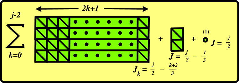
Figure 10: Oscillator modes of the orientifold matrix model expanded around the single-membrane vacuum. These $j+1$ superdiagrams correspond to a single-column $2j$-box superdiagram of the $\mathop{\rm SU}\nolimits(4|2)$ theory. The full spectrum, excluding $\lambda^{r}_{m}$, is obtained by summing also over $j$ with $1\leq j\leq N$.

A similar analysis could be made for the multimembrane vacua, starting from the data of Table 2. Note however that in the multimembrane vacua we must be careful to account for a possible residual gauge invariance: if there are several coincident membranes ($N_{k}=N_{l}$) then there is a subgroup of ${\mathrm{O}}(N)$ which leaves the classical solution (52) invariant, and the oscillators acting on physical states must be symmetrized over this subgroup. This guarantees that the indistinguishable membranes obey the correct statistics, essentially because $S_{N}$ is a subgroup of ${\mathrm{O}}(N)$.

7.4 Giant gluons

Let us return our attention to the simplest $E_{8}$ multiplet constructed above in (100), (101). These states are $\mathop{\rm SU}\nolimits(4|1)$ singlets with $J=\frac{\mu}{2}$, that is,

$$M^{12}=-1,\qquad M_{45}=M_{67}=M_{89}=0.$$ (103)

By acting on them with the kinematical supercharges we can get other polarizations. Namely, the operators $q^{I\dagger}$ are a spinor of $\mathop{\rm SO}\nolimits(6)$ and raise $M^{12}$ by $\frac{1}{2}$; then one can check that acting on (103), the $q^{I\dagger}$ produce the quantum numbers of the vector multiplet

$$\textbf{8}_{v}\oplus\textbf{8}_{s}$$ (104)

of ${\mathcal{N}}=1,d=10$ super Yang-Mills, propagating in the plane $x^{3}=0$.

Furthermore, as we saw in the last subsection, all of these vector multiplet states have energies which are perturbatively protected. For the ground state, which is an $\mathop{\rm SU}\nolimits(4|1)$ singlet, this follows from the fact that the singlet representation is an atypical representation. Then for the other states obtained by acting with $q^{I\dagger}$ note that $q^{I\dagger}$ belongs to the decoupled $\mathop{\rm{}U}\nolimits(1)\subset\mathop{\rm{}U}\nolimits(N)$ sector, hence has no corrections to its energy, so the absence of perturbative corrections should hold just as for the ground state. Note however that the energies are not all equal to the $\frac{\mu}{3}$ we found for the ground state; rather, by (39) and (42) each $q^{I\dagger}$ increases $H$ by $\frac{\mu}{4}$, so the energies range from $\frac{\mu}{3}$ to $\frac{4\mu}{3}$ according to the rule

$$H=\mu\left(\frac{5}{6}+\frac{1}{2}M^{12}\right).$$ (105)

In sum, we have found states of the hemispherical membrane which transform in the $\bf{248}$ of $E_{8}$ and have the quantum numbers of the $d=10$ vector multiplet, with light-cone energies given by (105) to all orders perturbatively in $R/\mu$; we call these states giant gluons. Recalling that our matrix model describes DLCQ of M-theory on the orientifolded plane wave, these giant gluon states should be identified with one-gluon states of the gauge field which propagates in the $X^{3}=0$ plane. Similarly, multi-gluon states are identified with states containing several membranes.

7.5 Giant gravitons

The appearance of giant gluons here is analogous to that of giant gravitons in the BMN model; in that case there were 16 kinematical supercharges and their quantization gave the full graviton multiplet through the ground state degeneracy of the spherical membrane. In our model the graviton multiplet is harder to see explicitly because we have only 8 kinematical supercharges. Acting with these supercharges on the even $N$ ground state generates only 16 states with protected energies, which was sufficient for the giant gluons but is not sufficient to produce the whole graviton multiplet. Some components of the $\mu=0$ graviton may indeed have quantum corrections to their masses at finite $\mu$, and disappear from the spectrum altogether at $\mu=\infty$.

7.6 The $\mu\to 0$ limit

As we have emphasized, one of the advantages of working at finite $\mu$ is that the problems associated with flat directions in the potential are absent and one can identify multiparticle states easily. In particular, we have found states which are candidates for single- and multiple-gluon states in the DLCQ description of M-theory in the plane wave background. One might ask whether we can use these states to solve the original problem of identifying the multiple-gluon bound states at $\mu=0$ (or at least to prove their existence.) In fact, one could ask a similar question already for the graviton states in the BMN matrix model. There are two potential difficulties. One is that with $16$ supercharges our representation-theory arguments are only strong enough to show that the energies are protected perturbatively in $R/\mu$. But even if we assume that we can identify the required states at any nonzero $\mu$, with protected energies, there is a more formidable difficulty: these states may become non-normalizable in the $\mu\to 0$ limit. So it seems that our analysis does not allow us to say anything directly about the existence of bound states in the $\mu=0$ case; the latter problem still requires more subtle analytical tools.

8 The fivebrane picture

8.1 Transverse fivebranes in the BMN model

It was argued in [22] that when the effective coupling about a membrane vacuum becomes large there is a dual description in terms of transverse fivebranes, which have topology $S^{5}$ and are extended in the $X^{a}$ directions. More concretely, consider the membrane vacuum $(1,1,\dots;2,2,\dots;k,k,\dots,k)$ where the $\mathop{\rm SU}\nolimits(2)$ representation of size $l$ is repeated $M_{l}$ times (hence $\sum_{l=1}^{k}lM_{l}=N$). In the large $N$ limit when $\frac{M_{l}}{N}$ is held fixed, the membrane theory about this vacuum becomes strongly coupled. However, this large $N$ limit has an alternative description as $k$ concentric fivebranes, with radii

$$\left((R_{l})_{M5}\right)^{4}=\frac{\mu}{6R}\sum_{i=l}^{k}M_{i},$$ (106)

and this dual fivebrane description is weakly coupled and perturbative [22]. In particular, with the above prescription, the trivial $X=0$ vacuum, i.e. $(1,1,\cdots,1)$, corresponds to a single membrane of radius $R_{M5}^{4}={\mu N}/(6R)$. In [22] it was checked that the BPS spectrum of $k$ non-coincident fivebranes, which is essentially $k$ copies of the spectrum of geometric fluctuations of a spherical fivebrane plus an Abelian self-dual two-form for each fivebrane, can be found among the spectrum of exactly protected states of the BMN matrix model.

8.2 Classical fivebranes in the orientifolded plane wave background

Now we want to make a similar analysis in the orientifolded theory. We begin by working out the classical spectrum which we will try to reproduce in the matrix model. First note that the classical $M5$-brane action on the orientifolded plane wave background in light-cone gauge has a zero-energy configuration corresponding to an $S^{5}$ extended in the $x^{a}$ directions with all $x^{i}=0$; in particular, $x^{3}=0$, so the spherical fivebrane is immersed in the Hořava-Witten domain wall. This is a transverse fivebrane since it is extended on the light-cone time $x^{+}$ and five spatial directions but not on $x^{-}$.

Next one can work out the spectrum of geometric fluctuations of the spherical fivebrane (these are the ordinary geometric degrees of freedom obtained from the ${\mathbb{Z}}_{2}$ quotient, as opposed to the new dynamics arising from having the fivebrane embedded in the domain wall.) Since the calculation is essentially similar to that of Appendix B of [22] we do not repeat them here. The result is simply that the modes in the orientifolded theory are the ones from the parent theory which survive the ${\mathbb{Z}}_{2}$ projection. Among the bosonic excitations of the fivebrane spectrum, the fluctuations corresponding to $x^{-}$, $x^{1}$, $x^{2}$ and to the radial direction of $S^{5}$ remain, while $x^{3}$ and the self-dual two-form are projected out. Among the fermionic excitations, noting that they are doublets of $\mathop{\rm SU}\nolimits(2)$, half of them which have negative $\sigma^{3}$ eigenvalue are projected out. So the 8+8 degrees of freedom of the ${\mathcal{N}}=(2,0)$ tensor multiplet are reduced to the 4+4 of the ${\mathcal{N}}=(1,0)$ hypermultiplet.

8.3 Single fivebrane vacuum in the heterotic matrix model

In the BMN model, as discussed in [22], it was the $X=0$ vacuum—or equivalently the $(1,1,\dots,1)$ vacuum—that described a single fivebrane. One might guess that the $X=0$ vacuum also describes the fivebrane in our model. However, this idea immediately faces two serious problems:

• All modes of the $\lambda$ fermions are massless around the $X=0$ vacuum of the ${\mathrm{O}}(N)$ theory. By quantizing these $16N$ real fermions, we obtain a huge representation of ${\mathrm{O}}(16)\times{\mathrm{O}}(N)$ whose dimension is $2^{8N}$. In fact, it is not difficult to see how these states obtained by quantizing fermions in $({\bf 16},{\bf N})$ decompose under ${\mathrm{O}}(16)\times{\mathrm{O}}(N)$. One starts with the observation that the operator

  $$\lambda^{r}_{n}\lambda^{r}_{m}\lambda^{s}_{m}\lambda^{s}_{n}$$ (107)

  is related to the quadratic Casimir operator of ${\mathrm{O}}(N)$ because $\lambda^{r}_{[n}\lambda^{r}_{m]}$ is proportional to the generator $G_{mn}$ of ${\mathrm{O}}(N)$. But just by rearranging the fermions (107) is also related to the quadratic Casimir of ${\mathrm{O}}(16)$. A careful counting of signs and anticommutators reveals that in the more general case of the group ${\mathrm{O}}(M)\times{\mathrm{O}}(N)$—in our case $M=16$—we obtain the identity

  $$C^{(2)}_{{\mathrm{O}}(M)}(\lambda)+C^{(2)}_{{\mathrm{O}}(N)}(\lambda)=\frac{MN}{4}(M+N-2)$$ (108)

  So among the states obtained by quantizing the $\lambda$ fermions, smaller representations of ${\mathrm{O}}(N)$ are always correlated with larger representations of ${\mathrm{O}}(16)$ and vice versa. In particular, to obtain physical ground states we would want to look at the singlets under ${\mathrm{O}}(N)$, and these transform as a huge representation of ${\mathrm{O}}(16)$ whose quadratic Casimir increases with $N$. It seems that there is no sensible large $N$ limit.

• A related problem is that the ground state energy of the $(1,1,\dots,1)$ vacuum in the ${\mathrm{O}}(N)$ theory is $H_{0}=N\mu/3$. The reason is simply that we have a lot of contributions $\mu/3$ from the ground states of the $N$ one-dimensional fuzzy spheres, since $1$ is odd (see Section 7.1.) Since $H_{0}$ becomes infinite as $N\to\infty$, this means the $X=0$ sector contains no finite energy states in the large $N$ limit.

These problems have a simple resolution. The $(1,1,\dots,1)$ vacuum actually describes a “fractional M5-brane”—an object that does not exist! The real M5-brane is equivalent to an instanton (not a half-instanton) in the domain wall gauge theory, and it can always leave the domain wall. When it does so, its mirror image moves in the opposite direction. In other words, the fivebrane in heterotic M-theory arises from a pair of fivebranes in the original theory. This statement is related to the well-known fact that the D5-branes in Type I string theory carry $\mathop{\rm{}USp}\nolimits(2k)$ symmetry. Now we see that the relevant vacuum for a single fivebrane in the heterotic matrix model is the $(2,2,\dots,2)$ vacuum. All $\lambda^{r}_{m}$ are now massive, and therefore the vacuum is a singlet under ${\mathrm{O}}(16)\times{\mathrm{O}}(N)$; moreover, since $2$ is even, the ground state energy is $H_{0}=0$.

8.4 Spectrum of matrix model about the single fivebrane vacuum

Mode	${\cal H}$	$J$	Degeneracy
$\lambda^{r}_{-\frac{1}{2},k}$	$0$	$\frac{1}{4}$	$16$

Table 3: The $\lambda$ modes about the $(2,2,\dots,2)$ vacuum.

We would now like to study the excitations of the $(2,2,\dots,2)$ vacuum, which in the large $N$ limit we want to identify with a single transverse fivebrane. We switch notation so that $N$ is the number of $2$-dimensional fuzzy spheres, i.e. the gauge group is ${\mathrm{O}}(2N)$. The classical solution $(2,2,\dots,2)$ breaks ${\mathrm{O}}(2N)\to{\mathrm{O}}(N)$, so all excitations will have to be invariant under ${\mathrm{O}}(N)$.

Mode	${\cal H}$	$J$	Degeneracy
$x^{\{kl\}}_{00}$	$\frac{1}{6}$	$\frac{1}{6}$	$6$
$\eta^{\{kl\}}_{\frac{1}{2},\frac{1}{2}}$	$\frac{5}{12}$	$\frac{1}{6}$	$4$
$\beta^{\{kl\}}_{1,1}$	$\frac{2}{3}$	$\frac{1}{6}$	$1$
$\eta^{[kl]}_{\frac{1}{2},-\frac{1}{2}}$	$\frac{1}{12}$	$\frac{1}{3}$	$4$
$\beta^{[kl]}_{1,0}$	$\frac{1}{3}$	$\frac{1}{3}$	$1$
$\beta^{\{kl\}}_{1,-1}$	$0$	$\frac{1}{2}$	$1$

Table 4: The modes from the $\mathop{\rm{}U}\nolimits(1)\subset\mathop{\rm{}U}\nolimits(2)$ part of the BMN model about the $(2,2,\dots,2)$ vacuum after a ${\mathbb{Z}}_{2}$ projection.

It is easy to generalize the formalism of the irreducible $(2)$ vacuum to the $(2,2,\dots,2)$ vacuum: all the oscillators $x^{a}_{jm},\alpha_{jm},\beta_{jm},\chi^{I}_{jm},\eta^{I}_{jm}$ acquire two extra indices $k,l=1,2,\dots N$, for the unbroken gauge group ${\mathrm{O}}(N)$. Because the ${\mathrm{O}}(2N)$ matrix transposition also exchanges the indices $k,l$, the constraint that the oscillators with $j-m$ did not exist in the irreducible vacuum is generalized here to the condition that the oscillators with $j-m$ odd are antisymmetric in $kl$, which we indicate by the symbol $[kl]$ in the tables. On the other hand, the oscillators with $j-m$ even are symmetric matrices of ${\mathrm{O}}(N)$, which we indicate by the symbol $\{kl\}$.

Tables 3, 4 and 5 specialize Table 2 to the case of the $(2,2,\dots,2)$ vacuum. (Note that ${\cal H}$ and $J$ are always measured in units of $\mu$.) In Table 3 we have listed the $\lambda$ modes. The ${\mathrm{O}}(2N)$ index of $\lambda$ has been decomposed into $2\times N$ as $\lambda^{r}_{\pm\frac{1}{2},k}$; hereafter, for simplicity, we suppress the $\pm\frac{1}{2}$ and write $\lambda^{r}_{k}$ for the creation operator $\lambda^{r}_{-\frac{1}{2},k}$. In Table 4 we have listed the modes from the $\mathop{\rm{}U}\nolimits(1)\subset\mathop{\rm{}U}\nolimits(2)$ part of the BMN model; and in Table 5 we have listed the remaining modes from the BMN model.

$\!\begin{array}[]{|c|ccccc|cccc|ccc|cc|c|}\hline\cr\mathrm{Mode}&\alpha^{\{kl\}}_{00}\!&\chi^{\{kl\}}_{\frac{1}{2},\frac{1}{2}}\!&x^{\{kl\}}_{1,1}\!&\eta^{\{kl\}}_{\frac{3}{2},\frac{3}{2}}\!&\beta^{\{kl\}}_{2,2}\!&\chi^{[kl]}_{\frac{1}{2},-\frac{1}{2}}\!&x^{[kl]}_{1,1}\!&\eta^{[kl]}_{\frac{3}{2},\frac{1}{2}}\!&\beta^{[kl]}_{2,1}\!&x^{\{kl\}}_{1,-1}\!&\eta^{\{kl\}}_{\frac{3}{2},-\frac{1}{2}}\!&\beta^{\{kl\}}_{2,0}\!&\eta^{[kl]}_{\frac{3}{2},-\frac{3}{2}}\!&\beta^{[kl]}_{2,-1}\!&\beta^{\{kl\}}_{2,-2}\!\\ \hline\cr{\cal H}&\frac{1}{3}&\frac{7}{12}&\frac{5}{6}&\frac{13}{12}&\frac{4}{3}&\frac{1}{4}&\frac{1}{2}&\frac{3}{4}&1&\frac{1}{6}&\frac{5}{12}&\frac{7}{6}&\frac{1}{6}&\frac{5}{12}&0\\ \hline\cr J&\frac{1}{3}&\frac{1}{3}&\frac{1}{3}&\frac{1}{3}&\frac{1}{3}&\frac{1}{2}&\frac{1}{2}&\frac{1}{2}&\frac{1}{2}&\frac{2}{3}&\frac{2}{3}&\frac{2}{3}&\frac{5}{6}&\frac{5}{6}&1\\ \hline\cr\mathrm{Degen.}&1&4&6&4&1&4&6&4&1&6&4&1&4&1&1\\ \hline\cr\end{array}$

Table 5: The modes from the $\mathop{\rm SU}\nolimits(2)\subset\mathop{\rm{}U}\nolimits(2)$ part of the BMN model about the $(2,2,\dots,2)$ vacuum which survive the ${\mathbb{Z}}_{2}$ projection.

Now let us discuss the states which may be constructed from these oscillators. We write ${\mathcal{O}}^{kl}$ to denote an arbitrary symmetrized product of oscillators from Tables 4, 5. Each such ${\mathcal{O}}^{kl}$ is either symmetric or antisymmetric in $k,l$ according to whether it has an even or odd number of antisymmetric constituents. Then there are three ways to construct an operator which is an ${\mathrm{O}}(N)$ singlet: we can take $\mathop{\rm Tr}\nolimits{\mathcal{O}}^{\{kl\}}$, $\lambda^{r}_{k}{\mathcal{O}}^{\{kl\}}\lambda^{s}_{l}$, or $\lambda^{r}_{k}{\mathcal{O}}^{[kl]}\lambda^{s}_{l}$, giving respectively ${\bf 1}$, ${\bf 120}$, or ${\bf 135}\oplus{\bf 1}$ of $\mathop{\rm SO}\nolimits(16)$. We call all of these “one-oscillator” states even though some of them contain three oscillators. A general state is obtained by acting with some number of these singlet operators on the vacuum.

Figure 11: Two-box multiplet. This multiplet appears twice in the spectrum of one-oscillator states around the $(2,2,\dots,2)$ vacuum.

To see which of these states are protected, we should analyze the $\mathop{\rm SU}\nolimits(4|1)\times\mathop{\rm{}U}\nolimits(1)_{J}\times\mathop{\rm SO}\nolimits(16)$ multiplets in which they transform. However, as we described in Section 5, the mere fact that a particular state is in an atypical multiplet is not enough to ensure that it is protected; atypical multiplets whose number of boxes differ by three as shown in Figure 9 can in principle combine into a typical multiplet and receive corrections. Of course, in our case where each superdiagram is also carrying $J$ and $\mathop{\rm SO}\nolimits(16)$ quantum numbers, there is the extra condition that the multiplets which combine should have equal $J$ and $\mathop{\rm SO}\nolimits(16)$ quantum numbers.

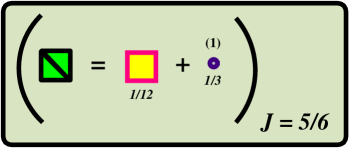
Figure 12: Single-box multiplet. This multiplet appears in the spectrum of one-oscillator states around the $(2,2,\dots,2)$ vacuum.

One-oscillator states

To get a feel for the situation, let us first discuss the one-oscillator states. First we consider states for which the one oscillator comes from Table 4. Their quantum numbers are as follows:

${\bullet}$ $\mathop{\rm Tr}\nolimits\beta_{1,-1}|0\rangle\$ is an $\mathop{\rm SU}\nolimits(4|1)$ singlet with $J=\frac{1}{2}$.

${\bullet}$ $\mathop{\rm Tr}\nolimits x_{00}|0\rangle\$ is the highest weight state of a $\mathop{\rm SU}\nolimits(4|1)$ two-box representation, shown in Figure 11, with $J=\frac{1}{6}$.

${\bullet}$ $\lambda^{r}_{k}\eta^{[kl]}_{\frac{1}{2},-\frac{1}{2}}\lambda^{s}_{l}|0\rangle$ and $\lambda^{r}_{k}\beta^{[kl]}_{1,0}\lambda^{s}_{l}|0\rangle$, both in ${\bf 135\oplus 1}$ of $\mathop{\rm SO}\nolimits(16)$, form a single box representation of $\mathop{\rm SU}\nolimits(4|1)$ with $J=\frac{5}{6}$, shown in figure 12.

${\bullet}$ $\lambda^{r}_{k}\beta^{\{kl\}}_{1,-1}\lambda^{s}_{l}|0\rangle$ is in the ${\bf 120}$ of $\mathop{\rm SO}\nolimits(16)$, $\mathop{\rm SU}\nolimits(4|1)$ singlet, with $J=1$.

${\bullet}$ $\lambda^{r}_{k}x^{\{kl\}}_{0,0}\lambda^{s}_{l}|0\rangle$ is in the ${\bf 120}$ of $\mathop{\rm SO}\nolimits(16)$ and is the highest weight state of a $\mathop{\rm SU}\nolimits(4|1)$ doublet, like that pictured in Figure 11 except that it has $J=\frac{2}{3}$.

Next consider the states for which the one oscillator comes from Table 5. These are summarized in Figures 13, 14.

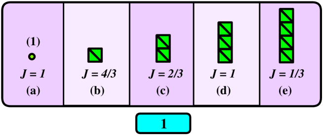
Figure 13: Multiplets built from a single oscillator of Table 5 which are $\mathop{\rm SO}\nolimits(16)$ singlets. The highest weight states of these multiplets are: (a) $\mathop{\rm Tr}\nolimits\beta_{2,-2}|0\rangle$; (b) $\lambda^{r}\eta_{\frac{3}{2},-\frac{3}{2}}\lambda^{r}|0\rangle$; (c) $\mathop{\rm Tr}\nolimits x_{1,-1}|0\rangle$; (d) $\lambda^{r}\chi_{\frac{1}{2},-\frac{1}{2}}\lambda^{r}|0\rangle$; (e) $\mathop{\rm Tr}\nolimits\alpha_{0,0}|0\rangle$. Note that except (e) all the multiplets are atypical.

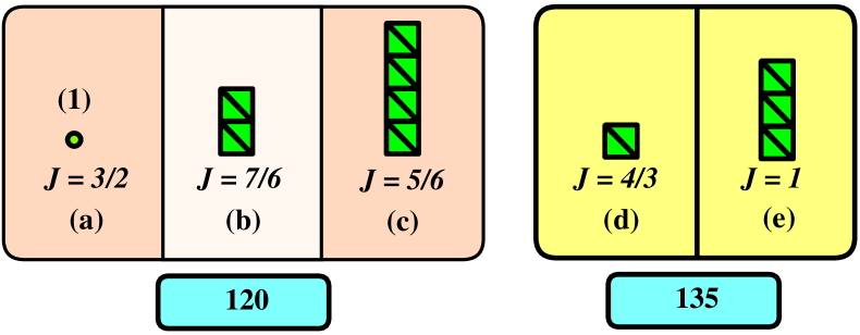
Figure 14: Multiplets built from a single oscillator of Table 5 which are in ${\bf 120}$ of $\mathop{\rm SO}\nolimits(16)$ (a, b, c) or ${\bf 135}$ of $\mathop{\rm SO}\nolimits(16)$ (d, e). The highest weight states of these multiplets are: (a) $\lambda^{r}\beta_{2,-2}\lambda^{s}|0\rangle$; (b) $\lambda^{r}x_{1,-1}\lambda^{s}|0\rangle$; (c) $\lambda^{r}\alpha_{0,0}\lambda^{s}|0\rangle$. (d) $\lambda^{r}\eta_{\frac{3}{2},-\frac{3}{2}}\lambda^{s}-\frac{1}{16}\delta^{rs}\lambda^{p}\eta_{\frac{3}{2},-\frac{3}{2}}\lambda^{p}|0\rangle$; (e) $\lambda^{r}\chi_{\frac{1}{2},-\frac{1}{2}}\lambda^{s}-\frac{1}{16}\delta^{rs}\lambda^{r}\chi_{\frac{1}{2},-\frac{1}{2}}\lambda^{r}|0\rangle$.

Having listed all the one-oscillator states we learn two lessons. One is that in contrast to the irreducible vacuum, the $(2,2,\dots,2)$ vacuum can support excitations corresponding to superdiagrams of $\mathop{\rm SU}\nolimits(4|1)$ with an odd number of boxes. As a result it is possible for diagrams to combine and the second lesson is that indeed this happens: for example, in Figure 13 the multiplets labeled (a) and (d) can combine to form a typical representation.

One can make a similar analysis for two-oscillator states, for which the representation content is obtained by symmetrized tensor products of the multiplets listed above. This analysis is described in Appendix A.

Protected states: geometric fluctuations of the fivebrane

In general we have seen that it is difficult to argue that an atypical multiplet is protected even perturbatively, nonetheless as we will argue some particular ones are. Consider the two-row atypical multiplet shown in Figure 15.

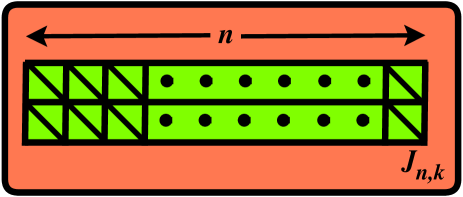
Figure 15: An atypical multiplet which occurs in the spectrum around the $(2,2,\dots,2)$ vacuum.

This multiplet occurs many times in the spectrum, with lowest $\mathcal{H}$ states

$$S_{a_{1}\cdots a_{n}}\mathop{\rm Tr}\nolimits\left(x_{00}^{a_{1}}\cdots x_{00}^{a_{n}}(\beta_{1,-1})^{k}\right)|0\rangle$$ (109)

where $S_{a_{1}\cdots a_{n}}$ is a totally symmetric traceless tensor of $\mathop{\rm SO}\nolimits(6)$. The state (109) is an $\mathop{\rm SO}\nolimits(16)$ singlet and has

$$J_{n,k}=\frac{n}{6}+\frac{k}{2}.$$ (110)

This is an atypical multiplet, but is it really protected? In fact, there is another multiplet in the spectrum which is a candidate to combine with it, namely the one with lowest $\mathcal{H}$ states

$$S_{a_{1}\cdots a_{n}}\lambda^{r}\left(\chi_{\frac{1}{2},-\frac{1}{2}}x_{00}^{a_{1}}\cdots x_{00}^{a_{n}}(\beta_{1,-1})^{l}\right)\lambda^{r}|0\rangle$$ (111)

This is again an $\mathop{\rm SO}\nolimits(16)$ singlet, has $\mathop{\rm SU}\nolimits(4|1)$ content given in Figure 16, and

$$J_{n,l}=\frac{n}{6}+\frac{l}{2}+1.$$ (112)

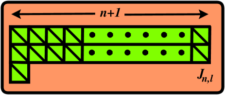
Figure 16: An atypical multiplet which could combine with the multiplet in Figure 15.

So for the two multiplets with highest weights (109), (111) to combine, we must have $k=l+2$. Hence the states (109) with $k\geq 2$ are not protected, but the ones with $k=0,1$ still could be protected. In fact they have no partners in the $\mu=\infty$ spectrum and hence their energies cannot receive any corrections in perturbation theory.

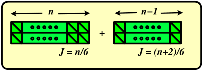
Figure 17: Two atypical representations which are exactly protected. The one with $2\times n$ boxes has ${\cal K}=0$ and the other one ${\cal K}=1$. These correspond to geometric fluctuations of the fivebrane.

Note that there are multiplets with the same $\mathop{\rm SU}\nolimits(4|1)$ representation content as shown in Figure 15, but with a different highest weight state, e.g.

$$S_{a_{1}\cdots a_{n}}\mathop{\rm Tr}\nolimits\left(x_{00}^{a_{1}}\cdots x_{00}^{a_{n-2}}x_{1,-1}^{a_{n-1}}x_{1,-1}^{a_{n}}\right)|0\rangle.$$ (113)

However, all such multiplets would have $J>\frac{n+2}{6}$ and hence, as we argued above, they have potential partners in the spectrum with which they can combine to form typical multiplets; therefore they are not protected.

So we have shown that the atypicals of the form shown in Figure 17 are perturbatively protected, i.e. one cannot find any multiplets with which they could combine in the spectrum of the matrix model about the $(2,2,\cdots,2)$ vacuum.

In fact, they are protected even nonperturbatively. To see this one has to check two things: first, that the partners of these states do not appear about any vacuum of the matrix model at $\mu=\infty$; second, that no typical multiplet appears which could split at finite $\mu$ into one of the partners of these states. Both of these can be checked directly by looking at the oscillator content of the theory. For this purpose it is convenient to exploit the label ${\cal K}$ defined in Section 5.4, which we recall:

$${\cal K}={\cal H}+2J-\frac{\mu}{2}M^{45}.$$ (114)

This ${\cal K}\geq 0$ for all oscillators in the theory, and the multiplets depicted in Figure 15 have

$${\cal K}=\frac{\mu n}{6}+2\mu\left(\frac{n}{6}+\frac{k}{2}\right)-\frac{\mu}{2}n=\mu k.$$ (115)

So $k=0,1$ are relatively hard to make; for these values there are not many states carrying ${\cal K}=k\mu$ and one can check directly that they do not form the dangerous multiplets which could give corrections to the ones in which we are interested. (This argument does not directly use the supersymmetric index of Section 5.4.)

Now let us focus on the state content of our protected multiplets, shown in Figure 17, and compare it with the spectrum of geometric fluctuations of a fivebrane (discussed in Section 8.2.) The expansion of a $2\!\times\!n$-box superdiagram has been shown in Figure 21. The highest-$\mathcal{H}$ sector of the $2\!\times\!n$-box and the lowest-$\mathcal{H}$ sector of the $2\!\times\!(n-1)$-box diagram correspond to the fluctuations of a fivebrane along the $x^{-}$ and radial directions, whereas the highest weight state of the $2\!\times\!(n-1)$-box diagram and the lowest weight state of the $2\!\times\!n$-box diagram correspond to fluctuations along $x^{1}$ and $x^{2}$. The remaining fermions match with the fermionic fluctuations of the fivebrane. We note that all these states are singlets of $\mathop{\rm SO}\nolimits(16)$.

Although we have not identified the complete spectrum of protected operators on either side, the matching of a natural class of protected operators constitutes some evidence that the $(2,2,\dots,2)$ vacuum describes the transverse fivebrane embedded in the domain wall, similar to the evidence presented in [22] in the case of the BMN matrix model. We can also make a conjecture about the multi-fivebrane vacua; following [22] it would be natural to consider the vacuum $(2,2,\dots,2;4,4,\dots,4;\dots;2k,2k,\dots,2k)$ as a $k$-fivebrane state. One could find evidence for this conjecture by looking for $k$ copies of the spectrum in Figure 17 in this vacuum.

8.5 The $(1,0)$ superconformal field theory

In 11-dimensional flat space with a Hořava-Witten domain wall, the low energy dynamics of a single fivebrane embedded in the domain wall are described by a $(1,0)$ superconformal field theory in six dimensions. We have found a vacuum of our matrix model which is a candidate to describe a large fivebrane embedded in the domain wall with topology $S^{5}$. We could try to identify the states around this vacuum with states of the SCFT defined on $S^{5}\times{\mathbb{R}}$; by the state-operator correspondence, this should give the operator spectrum of that theory, with dimensions $\Delta$ given by the rule

$$H\leftrightarrow\frac{\mu}{6}\Delta.$$ (116)

This rule can be justified by the usual logic of the state-operator correspondence: namely, when we put the conformal theory on an $S^{5}$ of radius $R_{5}$, we should identify $R_{5}\frac{\partial}{\partial t}$ with $\Delta$, where $t$ denotes the proper time. At large $\mu$ the proper time is dominated by the contribution from $(dx^{+})^{2}$ in the plane wave metric (1), giving $dt=\frac{\mu}{6}R_{5}dx^{+}$, so that

$$H=\frac{\partial}{\partial x^{+}}=\frac{\mu}{6}R_{5}\frac{\partial}{\partial t}=\frac{\mu}{6}\Delta,$$ (117)

as desired.

This identification could also have been made in the case of the BMN matrix model and the $(2,0)$ theory. Encouragingly, it seems to be reasonable there. Namely, in the $(2,0)$ theory one builds operators from the scalar fields $X^{i}$ representing transverse fluctuations, of mass dimension $2$, and the derivative operators $\partial^{a}$ which have mass dimension $1$; this corresponds to the fact that in the fivebrane vacuum of the BMN matrix model one has $\beta_{1m}$ with $H=\frac{\mu}{3}$ and $x^{a}_{00}$ with $H=\frac{\mu}{6}$.

So it would be interesting to see whether we can reproduce the operator spectrum of the $(1,0)$ theory using the fivebrane vacuum of our matrix model. The $(1,0)$ spectrum has been studied using AdS/CFT in [28] where the operators in short multiplets were classified by their $\mathop{\rm SO}\nolimits(4)\times E_{8}$ quantum numbers. We can make a few preliminary remarks about this problem. Indeed, essentially by repeating the procedure from Section 7.2 we can find states which, when completed to $\mathop{\rm SO}\nolimits(4)$ multiplets (this is necessary because the $\mathop{\rm SO}\nolimits(4)$ is not manifest after the pp-wave limit) would be candidates to match operators found in [28] transforming in the $(\textbf{3},\textbf{1},\textbf{248})$ of $\mathop{\rm SU}\nolimits(2)_{R}\times\mathop{\rm SU}\nolimits(2)_{L}\times E_{8}$. These are particularly interesting operators because they are likely responsible for the transition from the Coulomb branch to the Higgs branch [36, 37], where the fivebrane dissolves into a finite size $E_{8}$ instanton, producing $30$ hypermultiplets which parameterize the moduli space of $E_{8}$ instantons.

However, if indeed our matrix model can describe the $(1,0)$ theory the full story must be subtle, because we also find a puzzle: it seems to be impossible to find the $E_{8}$ symmetry in the full large $\mu$ spectrum of the matrix model. In particular, in the matrix model we can construct the state $\lambda^{r}_{-\frac{1}{2}}\eta_{\frac{1}{2},-\frac{1}{2}}\lambda^{s}_{-\frac{1}{2}}|0\rangle$ which has $H={7\mu}/{12}$ and transforms in the $\bf{135\oplus 1}$ of $\mathop{\rm SO}\nolimits(16)$; but we have not found a way to complete the 135 to a multiplet of $E_{8}$. The smallest candidate is 3875 but this would require us to find the $\bf{1820\oplus 1920}$ of $\mathop{\rm SO}\nolimits(16)$ elsewhere in the spectrum at $H={7\mu}/{12}$, and we have not found a way to construct these states. They might arise in a rather complicated way — already in the membrane vacuum we had to use both even and odd $N$ sectors to fill out the $E_{8}$ multiplets, so in the fivebrane case we might have to combine various vacua which are close to $(2,2,\dots,2)$ in some appropriate sense.

In sum, further study will be required to see in what sense there is an $E_{8}$ symmetry in the fivebrane vacuum of our matrix model and whether our matrix model can describe the $(1,0)$ theory.

9 Conclusions and outlook

In this paper we showed that the plane-wave matrix models may be a powerful tool to answer many questions in M-theory. A simple system of harmonic oscillators allowed us to understand, the $E_{8}$ symmetry arising from membrane boundaries, the origin of giant gluons and anomaly cancellation in the membrane worldvolume; furthermore it seems to capture at least some of the degrees of freedom of the fivebrane embedded in the domain wall, and we may hope that indeed it will capture all of them. Clearly, we have not resolved all outstanding questions about heterotic M-theory. In particular, we have failed to clarify the following issues in the plane-wave matrix models, which in our opinion deserve further investigation:

• Understanding the $\mu\to 0$ limit. The $\mu\to 0$ limit is a highly nonperturbative regime from the viewpoint of the perturbative expansion of the plane-wave matrix model. Some states that are guaranteed to exist for finite $\mu$ become non-normalizable at $\mu=0$. It is desirable to find some machinery that allows us to prove that the “right” states survive and the others don’t. A full argument could use the supersymmetric indices combined with the $\mathop{\rm SO}\nolimits(8)$ rotational symmetry that gets restored for $\mu=0$ (or $\mathop{\rm SO}\nolimits(9)$ in the case of the BMN model).

• The spectrum of operators in the $(1,0)$ theory. As we discussed in Section 8.5, using the state-operator correspondence it might be possible to identify explicitly the operator spectrum of the $(1,0)$ theory by a careful study of the spectrum of our matrix model around the fivebrane vacuum. Because the plane-wave background breaks some of the symmetries, not all components of the R-symmetry multiplets survive to $\mu=\infty$. In our case, the $\mathop{\rm SO}\nolimits(4)$ R-symmetry was broken to $\mathop{\rm{}U}\nolimits(1)$ generated by $M^{12}$. Similarly, the $\mathop{\rm SO}\nolimits(5)$ R-symmetry of the $(2,0)$ theory was broken to $\mathop{\rm SO}\nolimits(3)$ in the BMN case. It might be possible to find a way to identify the rest of the operator spectrum or at least a well-defined rule that would determine which operators are visible in the matrix model and how many “invisible” (i.e. unprotected) operators there are. One might also try to understand whether there is some relation between our matrix model, in which the fivebrane arises dynamically, and the matrix models describing longitudinal flat fivebranes [38, 39]. Finally, it might be possible to exhibit explicitly the $E_{8}$ symmetry which should be there in the $(1,0)$ theory, although as discussed in Section 8.5 this will apparently require some new idea.

• A more complete proof of the $E_{8}$ symmetry for membranes at large $N$. We were able to show that the membrane spectrum at $\mu=\infty$ forms full representations of $E_{8}$. A more complete proof for finite $\mu$, including the interactions of membranes, might still result from an application of the techniques of two-dimensional CFT’s, in agreement with the dimension of the boundaries.

• More general backgrounds. There might be other backgrounds of M-theory that admit a matrix model description. For example, it might be interesting to study various supersymmetric orbifolds of the BMN plane wave, i.e. the massive deformations of the ALE spaces, as well as the matrix models for stringy pp-wave backgrounds.

Although the ultimate reach of these matrix models will most likely be limited to highly symmetric backgrounds similar to ours, we are hopeful that some general insights resulting from these models might have a broader range of validity.

Appendix A Two-oscillator states around the fivebrane vacuum

The one-oscillator states around the $(2,2,\dots,2)$ vacuum were discussed in the main text, in Section 8.4. We may similarly analyze the two-oscillator states, obtained by symmetric tensor multiplication of two single-oscillator superdiagrams. As an example we show the symmetric product of two such diagrams:

where

The first multiplet in the two-oscillator state decomposition is typical, while the other three are atypical.

Equipped with superdiagram multiplications, one can easily work out the two-oscillator states. The two oscillators may be chosen from Tables 4 or 5. All the two-oscillator states in which both oscillators come from Table 4 are shown in Figure 18.

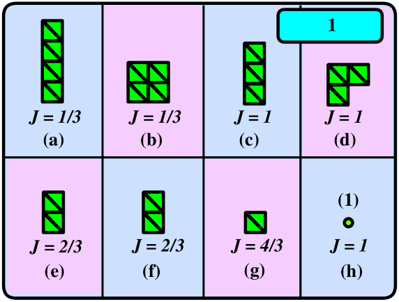
Figure 18: Two oscillator states of the $\mathop{\rm{}U}\nolimits(1)\subset\mathop{\rm{}U}\nolimits(2)$ sector of the ${\mathrm{O}}(2N)$ theory which are $\mathop{\rm SO}\nolimits(16)$ singlets. The highest weight state of these multiplets are: (a) $\mathop{\rm Tr}\nolimits(x^{a}_{00}x^{a}_{00})|0\rangle$; (b) $\mathop{\rm Tr}\nolimits(x^{a}_{00}x^{b}_{00}-\frac{1}{6}\delta_{ab}x^{c}_{00}x^{c}_{00})|0\rangle$; (c,d) $\lambda^{r}\eta_{\frac{1}{2},-\frac{1}{2}}x^{a}_{00}\lambda^{r}|0\rangle$; (e) $\mathop{\rm Tr}\nolimits(\eta_{\frac{1}{2},-\frac{1}{2}}\eta_{\frac{1}{2},-\frac{1}{2}})|0\rangle$; (f) $\mathop{\rm Tr}\nolimits(x^{a}_{00}\beta_{1,-1})|0\rangle$; (g) $\lambda^{r}\eta_{\frac{1}{2},-\frac{1}{2}}\beta_{1,-1}\lambda^{r}|0\rangle$; (h) $\mathop{\rm Tr}\nolimits(\beta_{1,-1}\beta_{1,-1})|0\rangle$. Note that except (a) all the multiplets are atypical.

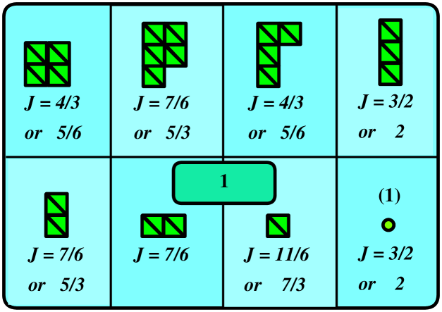
Figure 19: Two oscillator atypical multiplets of the ${\mathrm{O}}(2N)$ theory which are $\mathop{\rm SO}\nolimits(16)$ singlets.

One may similarly construct states involving one oscillator of Table 4 and one oscillator of Table 5 or two oscillators of Table 5. These states may be in ${\bf 1,120}$ or ${\bf 135}$ of $\mathop{\rm SO}\nolimits(16)$. In Figure 19 we have gathered the atypical multiplets from the rest of the two-oscillator states about the $(2,2,\cdots,2)$ vacuum which are $\mathop{\rm SO}\nolimits(16)$ singlets (several more two-oscillator atypicals have already been depicted in Figure 18).

As we see from Figures 18 and 19, many of these atypical representations can find partners to combine with and receive energy shifts. The $2\times 2$-box diagram with $J={4}/{3}$ can also find its partner (which is the $(0,2,1|0)$ multiplet) among the three oscillator states and hence it is also not protected.

The above discussion generalizes in an obvious way to $m$-oscillator states; we find typical multiplets as well as atypical ones; for example, some of the $n+k$-oscillator states which are relevant for the fivebrane interpretation have been shown in Figure 15.

Figure 20: Some examples of the simplest $\mathop{\rm SU}\nolimits(4|1)$ superdiagrams and their decomposition under $\mathop{\rm SU}\nolimits(4)$. The slashed boxes represent superindices while the ordinary boxes are $\mathop{\rm SU}\nolimits(4)$ indices. Bosonic representations are shaded in grey and fermionic representations are shaded yellow.

References

- [1] E. Witten, “String theory dynamics in various dimensions,” Nucl. Phys. B 443 (1995) 85 [hep-th/9503124].
- [2] T. Banks, W. Fischler, S. H. Shenker and L. Susskind, “M theory as a matrix model: A conjecture,” Phys. Rev. D 55 (1997) 5112 [hep-th/9610043].
- [3] B. de Wit, J. Hoppe and H. Nicolai, “On The Quantum Mechanics Of Supermembranes,” Nucl. Phys. B 305 (1988) 545.
- [4] L. Susskind, “Another conjecture about M(atrix) theory,” arXiv:hep-th/9704080.
- [5] S. Sethi and M. Stern, “D-brane bound states redux,” Commun. Math. Phys. 194 (1998) 675 [hep-th/9705046].
- [6] M. Porrati and A. Rozenberg, “Bound states at threshold in supersymmetric quantum mechanics,” Nucl. Phys. B 515 (1998) 184 [hep-th/9708119].
- [7] L. Motl, “Proposals on nonperturbative superstring interactions,” [hep-th/9701025].
- [8] T. Banks and N. Seiberg, “Strings from matrices,” Nucl. Phys. B 497 (1997) 41 [hep-th/9702187].
- [9] R. Dijkgraaf, E. Verlinde and H. Verlinde, “Matrix string theory,” Nucl. Phys. B 500 (1997) 43 [hep-th/9703030].
- [10] U. H. Danielsson and G. Ferretti, “The heterotic life of the D-particle,” Int. J. Mod. Phys. A 12, 4581 (1997) [hep-th/9610082].
- [11] L. Motl, “Quaternions and M(atrix) theory in spaces with boundaries,” [hep-th/9612198].
- [12] N. Kim and S. J. Rey, “M(atrix) theory on an orbifold and twisted membrane,” Nucl. Phys. B 504 (1997) 189 [hep-th/9701139].
- [13] T. Banks, N. Seiberg and E. Silverstein, “Zero and one-dimensional probes with supersymmetry,” Phys. Lett. B 401 (1997) 30 [hep-th/9703052].
- [14] T. Banks and L. Motl, “Heterotic strings from matrices,” J. High Energy Phys. 9712 (1997) 004 [hep-th/9703218].
- [15] D. A. Lowe, “Heterotic matrix string theory,” Phys. Lett. B 403 (1997) 243 [hep-th/9704041].
- [16] S. J. Rey, “Heterotic M(atrix) strings and their interactions,” Nucl. Phys. B 502 (1997) 170 [hep-th/9704158].
- [17] P. Hořava, “Matrix theory and heterotic strings on tori,” Nucl. Phys. B 505 (1997) 84 [hep-th/9705055].
- [18] P. Hořava and E. Witten, “Heterotic and type I string dynamics from eleven dimensions,” Nucl. Phys. B 460 (1996) 506 [hep-th/9510209].
- [19] P. Hořava and E. Witten, “Eleven-Dimensional Supergravity on a Manifold with Boundary,” Nucl. Phys. B 475 (1996) 94 [hep-th/9603142].
- [20] D. Berenstein, J.M. Maldacena and H. Nastase, “Strings in flat space and PP waves from super Yang-Mills,” J. High Energy Phys. 04 (2002) 013 [hep-th/0202021].
- [21] J. McGreevy, L. Susskind and N. Toumbas, “Invasion of the giant gravitons from anti-de Sitter space,” J. High Energy Phys. 0006 (2000) 008 [hep-th/0003075].
- [22] J. Maldacena, M. M. Sheikh-Jabbari and M. Van Raamsdonk, “Transverse fivebranes in matrix theory,” J. High Energy Phys. 0301 (2003) 038 [hep-th/0211139].
- [23] T. Banks, N. Seiberg and S. H. Shenker, “Branes from matrices,” Nucl. Phys. B 490 (1997) 91 [hep-th/9612157].
- [24] M. Blau, J. Figueroa-O’Farrill, C. Hull and G. Papadopoulos, “Penrose limits and maximal supersymmetry,” Class. and Quant. Grav. 19 (2002) L87 [hep-th/0201081].
- [25] K. Dasgupta, M. M. Sheikh-Jabbari and M. Van Raamsdonk, “Matrix perturbation theory for M-theory on a PP-wave,” J. High Energy Phys. 0205 (2002) 056 [hep-th/0205185].
- [26] K. Dasgupta, M. M. Sheikh-Jabbari and M. Van Raamsdonk, “Protected multiplets of M-theory on a plane wave,” J. High Energy Phys. 0209 (021) 2002 [hep-th/0207050].
- [27] N. Kim and J. Plefka, “On the spectrum of pp-wave matrix theory,” Nucl. Phys. B 643, 31 (2002) [arXiv:hep-th/0207034].
- [28] E. G. Gimon and C. Popescu, “The operator spectrum of the six-dimensional (1,0) theory,” J. High Energy Phys. 04 (1999) 018 [hep-th/9901048].
- [29] N. Kim and J. H. Park, “Superalgebra for M-theory on a pp-wave,” Phys. Rev. D 66, 106007 (2002) [arXiv:hep-th/0207061].
- [30] V. G. Kac, Representations Of Classical Lie Superalgebras, in Bonn 1977, proceedings of differential geometrical methods in mathematical physics 2, Berlin 1977, pp. 597-626; Lie Superalgebras, Adv. Math. 26 (1977) 8.
- [31] I. Bars, Supergroups And Their Representations, Lectures Appl. Math. 21, 17 (1983). A. Baha Balantekin and I. Bars, Branching Rules For The Supergroup SU(N/M) From Those Of SU(N+M), J. Math. Phys. 23, 1239 (1982).
- [32] I. Bars, B. Morel and H. Ruegg, Kac-Dynkin Diagrams And Supertableaux, J. Math. Phys. 24, 2253 (1983).
- [33] E. Witten, “Constraints On Supersymmetry Breaking,” Nucl. Phys. B 202 (1982) 253.
- [34] S. Kachru and E. Silverstein, “On gauge bosons in the matrix model approach to M theory,” Phys. Lett. B 396 (70) 1997 [hep-th/9612162].
- [35] L. Motl and L. Susskind, “Finite N heterotic matrix models and discrete light cone quantization,” [hep-th/9708083].
- [36] O. J. Ganor and A. Hanany, “Small Instantons and Tensionless Non-critical Strings,” Nucl. Phys. B 474 (1996) 122 [hep-th/9602120].
- [37] N. Seiberg and E. Witten, “Comments on String Dynamics in Six Dimensions,” Nucl. Phys. B 471 (1996) 121 [hep-th/9603003].
- [38] O. Aharony, M. Berkooz, S. Kachru, N. Seiberg and E. Silverstein, “Matrix description of interacting theories in six dimensions,” Adv. Theor. Math. Phys. 1 (1998) 148 [hep-th/9707079].
- [39] O. Aharony, M. Berkooz, S. Kachru and E. Silverstein, “Matrix description of (1,0) theories in six dimensions,” Phys. Lett. B 420, 55 (1998) [hep-th/9709118].