Constructing dark energy models with late time de Sitter attractor

Abstract

ABSTRACT: In this paper, we describe a way to construct a class of dark energy models that admit late time de Sitter attractor solution. In the canonical scalar and Born-Infeld scalar dark energy models, we show mathematically that a simple sufficient condition for the existence of a late time de Sitter like attractor solution is that the potentials of the scalar field have non-vanishing minimum while this condition becomes that the potentials have non-vanishing maximum for the phantom models. These attractor solutions correspond to an equation of state $w=-1$ and a cosmic density parameter $\Omega_{\phi}=1$, which are important features for a dark energy model that can meet the current observations.

I. Introduction

Current observations converge on that roughly two thirds of the energy density in our universe is resulted from a kind of dark energy that has negative pressure and can drive the accelerating expansion of the universeriess ; perlmutter ; bennett ; Netterfield ; Halverson . Many candidates for dark energy have been proposed so far to fit the current observations. Among these models, the most typical ones are cosmological constant and a time varying scalar field with positive or negative kinetic energy evolving in a specific potential, referred to as ”quintessence”ratra ; Coble ; Steinhardt ; Peebles or ”phantom”caldwell ; Carroll ; Frampton ; hao1 ; li1 ; Gibbons ; Feinstein ; Sami . Successful dark energy models also share some common features: (i) they should have an effective equation of state $w<-1/3$ so as to accelerate the expansion of the universe at recent epoch. (ii) they should be negligible compared with radiation and matter in the early epoch of the universe so as not to affect the primordial nucleosynthesis while dominate over the matter in a very recent epoch. (iii) they should not be very sensitive to the initial conditions so as to alleviate the fine tuning problems. Most emphasis in the literatures is on the question of determining the evolution of equation of state $w$. The purpose of this paper is to clarify that the minimum (maximum for the phantom models) of the potential corresponding to a cosmological de Sitter phase is a dynamical attractor, to which a wide range of initial values will converge.

The dynamical system of the scalar field with canonical Lagrangian have been widely studiedattractor , among which the global structure of the phase plane has been investigated and various critical points and their physical significances have been identified and manifested. However, in this paper, we focus on the late time de Sitter attractor solution and give a very simple sufficient condition for its existence. There are two major motivations to study the dark energy models that have late time de Sitter attractor. Firstly, a model will become very interesting if its dynamical system admits a late time attractor solution that leads to an equation of state $w=-1$ and a cosmic density parameter $\Omega_{\phi}=1$, which meet all the above 3 points. In this paper, we will show that if the potential of a model with positive kinetic energy (quintessence) has non-vanishing minimum, or the potential of a model with negative kinetic energy (phantom) has non-vanishing maximum, the dynamical system of the model will admit late time attractor solutions corresponding to $w=-1$ and $\Omega_{\phi}=1$. The subsequent numerical study on some specific models confirm the above conclusion. Secondly, recent observations do not exclude, but actually suggest an equation of state $-1.38<w<-0.82$Melchiorri . A striking consequence of dark energy with $w<-1$ is that the Universe will undergo a catastrophic ”big rip” in a finite timebigrip ; McInnes . If dark energy is characterized by an equation of state $w<-1$ (referred to as phantom in literatures) then the phantom energy density is still positive though it will first increase from a finite value up to infinite in a finite cosmic time, thereafter steadily decreases down to zero as cosmic time goes to infinity. To a fundamental observer in our galaxy, this state coincides with the above-mentioned big rip. However, in the case that there is a de Sitter attractor at late time, one can expect that the evolution of the scale factor recovers a rather conventional pattern, without big rip phase. de Sitter attractor will prevent the phantom energy density from increasing up to infinite in a finite cosmic time. Therefore, the presence of phantom energy does not lead to such a cosmic doomsday in a theory with de Sitter attractor at late time.

The paper is organized as follows: In sections II and III, a sufficient condition for dark energy with late time de Sitter attractor for the canonical scalar field models without and with internal O(N) symmetry was given. In section IV, the scalar field model in Born-Infeld type Lagrangian is discussed. In section V, the counterparts of the models in Section II, III and IV in the phantom scheme (with negative kinetic energy) have been investigated and the attractor behavior is manifested. In section VI, we numerically investigate some specific models and confirm the conclusion obtained in previous sections. Finally, in section VII, we present a discussion.

2. The scalar field model in canonical Lagrangian

In this section, we will study the case that the dark energy is mimicked by a scalar field expressed by canonical Lagrangian. We will work in the flat Robertson-Walker metric

$$ds^{2}=-dt^{2}+a^{2}(t)(dx^{2}+dy^{2}+dz^{2})$$ (1)

The equation of motion for the scalar field with canonical Lagrangian is

$$\ddot{\phi}+3H\dot{\phi}+\frac{\partial V(\phi)}{\partial\phi}=0$$ (2)

To gain more insights into the dynamical system, we introduce the new dimensionless variables

$$x =\frac{\phi}{\phi_{0}}$$

$$y =\frac{\dot{\phi}}{\phi_{0}^{2}}$$

$$N =\ln a$$ (3)

Then the above equations could be rewritten as

$$\frac{dx}{dN} =\frac{\phi_{0}y}{H}$$

$$\frac{dy}{dN} =-3y-\frac{V^{\prime}(x)}{\phi_{0}^{3}H}$$ (4)

where the prime denotes the derivative with respect to $x$ and $H$ is Hubble parameter that could be rewritten as

$$H^{2}=H_{i}^{2}E^{2}(N)$$ (5)

where $H_{i}$ denote the Hubble parameter at an initial time. $\Omega_{M,i}$ and $\Omega_{r,i}$ are the cosmic density parameters for matter and radiation at the initial time. We also choose the initial scale factor $a_{i}=1$. $E(N)$ is defined as

$$E(N)=\left[\frac{\kappa}{3H_{i}^{2}}\left(\frac{\phi_{0}^{4}y^{2}}{2}+V(x)\right)+\Omega_{M,i}e^{-3N}+\Omega_{r,i}e^{-4N}\right]^{1/2}$$ (6)

At late time, $N$ goes to be very large and the contribution from matter and radiation in Eq.(5) become negligible compared with the scalar field. To see this more clearly, we take the example that when the equation of state of the dark energy is constant and $w_{\phi}$ must be less than $-1/3$ so as to accelerate the expansion of the universe. Thus the dark energy component will evolve with $N$ as $\Omega_{\phi}e^{-3(1+w_{\phi})N}$, which dissipates slower than matter and radiation. So, at late time, we will have

$$\frac{dx}{dN} =\sqrt{\frac{3}{\kappa}}\frac{\phi_{0}y}{\sqrt{\phi_{0}^{4}y^{2}/2+V(x)}}$$

$$\frac{dy}{dN} =-3y-\sqrt{\frac{3}{\kappa}}\frac{V^{\prime}(x)}{\phi_{0}^{3}\sqrt{\phi_{0}^{4}y^{2}/2+V(x)}}$$ (7)

The critical point of the above autonomous system is $(x_{c},0)$, where $x_{c}$ is defined by $V^{\prime}(x_{c})=0$. Linearize the Eqs.(Constructing dark energy models with late time de Sitter attractor) about the critical point, we will have

$$\frac{dx}{dN} =\sqrt{\frac{3}{\kappa V(x_{c})}}\phi_{0}y$$

$$\frac{dy}{dN} =-\sqrt{\frac{3}{\kappa V(x_{c})}}\frac{V^{\prime\prime}(x_{c})x}{\phi_{0}^{3}}-3y$$ (8)

The eigenvalues of the system are

$$\lambda_{1,2}=\frac{-\alpha\pm\sqrt{\alpha^{2}-4\beta}}{2}$$ (9)

where $\alpha=3$ and $\beta=\frac{3V^{\prime\prime}(x_{c})}{\kappa V(x_{c})\phi_{0}^{2}}$. Now, we can conclude that for a positive potential $V(x)$, the critical point $(x_{c},0)$ is stable if $V^{\prime\prime}(x_{c})>0$. This is to say that the dynamical system has a stable critical point at the minimum of the potential and this critical point corresponds to a late time attractor solution. Especially, from Eq.(9), we can read that if $\beta<\alpha$ the critical point will be a stable node and it will be a stable spiral if $\beta>\alpha$. Although the relation between $\alpha$ and $\beta$ will not alter the stability property of the critical point, it will surely affect the way the field approaching the attractor. If the critical point is a stable spiral, the oscillation of the field will increase while for a stable node, the field will approach the attractor rather smoothly. These subtle properties have been further confirmed by the numerical analysis in section VI. Next, let’s read out the physical implications when the system is at the attractor regime. The cosmic density parameter for the dark energy is

$$\Omega_{\phi}=\frac{\kappa[\phi_{0}^{4}y^{2}/2+V(x)]}{3H_{i}^{2}E^{2}(N)}$$ (10)

and the equation of state of the scalar field is

$$w_{\phi}=\frac{\phi_{0}^{4}y^{2}-2V(x)}{\phi_{0}^{4}y^{2}+2V(x)}$$ (11)

Clearly, from Eq.(10) and Eq.(11), one can find that $w_{\phi}=-1$ and $\Omega_{\phi}=1$ at the late time attractor. Note that the energy density of the scalar field at the critical point is $V(x_{c})$ and should not vanish, thus the sufficient condition for the existence of a viable cosmological model with a late time de Sitter attractor solution should be that: the potential of the field has non-vanishing minimum.

III. The scalar field with internal O(N) symmetry in canonical Lagrangian

In this section, we devote ourselves to the scalar models in which the fields possess an internal symmetry. The complex scalar (with U(1) internal symmetry) field models were proposed by Gu and Huang and Boyle et. al.gu ; Boyle , and were generalized to the general case with an O(N) internal symmetry by Li, Hao and Liuli . The equation of motion for the O(N) scalar field is

$$\ddot{\phi}+3H\dot{\phi}-\frac{\Sigma^{2}}{a^{6}\phi^{3}}+V^{\prime}(\phi)=0$$ (12)

where the term $-\frac{\Sigma^{2}}{a^{6}\phi^{3}}$ is resulted from the internal symmetry and $\Sigma$ is an integration constantli . By using the dimensionless variables defined by Eq.(Constructing dark energy models with late time de Sitter attractor), we can write the equation of motion as

$$\frac{dx}{dN} =\frac{\phi_{0}y}{H}$$

$$\frac{dy}{dN} =-3y-\frac{V^{\prime}(x)}{\phi_{0}^{3}H}+\frac{\Sigma^{2}e^{-6N}}{\phi_{0}^{5}x^{3}H}$$ (13)

where $H$ is given by Eq.(5) but with a different

$$E(N)= \bigg{[}\frac{\kappa}{3H_{i}^{2}}\bigg{(}\frac{\phi_{0}^{4}y^{2}}{2}+\frac{\Sigma^{2}e^{-6N}}{2\phi_{0}^{2}x^{2}}$$ (14)

$$+V(x)\bigg{)}+\Omega_{M,i}e^{-3N}+\Omega_{r,i}e^{-4N}\bigg{]}^{1/2}$$

One can easily identify that the term $\frac{\Sigma^{2}e^{-6N}}{2\phi_{0}^{2}x^{2}}$ from the contribution of internal symmetry will decrease to be negligible at late time as well as the terms from matter and radiation. Thus, the autonomous system for the O(N) scalar fields Eqs.(Constructing dark energy models with late time de Sitter attractor) will reduce to Eqs.(Constructing dark energy models with late time de Sitter attractor) and the discussion in previous section concerning the single scalar field still hold true here. We will only write down the conclusion here: the O(N) scalar field models admit a late time attractor solution when the potential has non-vanishing minimum corresponding to $x_{c}\neq 0$. This is because the equation of motion Eqs.(12) will become singular at $x=0$ and therefore $x_{c}\neq 0$ is a constraint imposed by the O(N) symmetry. At the attractor regime, on can find that the cosmic energy parameter for the O(N) scalar fields is $\Omega_{\phi}=1$ and the equation of state is $w_{\phi}=-1$, which are the same as the single scalar field models except the process it approach the late time attractor.

IV. The scalar field model in Born-Infeld type Lagrangian

Recent work by Sen showed that the tachyon of string theory could be described by Born-Infeld type Lagrangian and its roles in inflation and dark energy have been studiedsen ; quint . So, it is also very interesting to consider the dark energy models with Born-Infeld type Lagrangian. The equation of motion for a scalar field with Born-Infeld type Lagrangian is

$$\ddot{T}+3H\dot{T}(1-\dot{T}^{2})+\frac{V^{\prime}(T)}{V(T)}(1-\dot{T}^{2})=0$$ (15)

By introducing the new dimensionless variables (Note that the field in Born-Infeld Lagrangian has different dimension from that in canonical Lagrangian)

$$x =\frac{T}{T_{0}}$$

$$y =\dot{T}$$ (16)

The equation of motion could be reduced to

$$\frac{dx}{dN} =\frac{y}{T_{0}H}$$

$$\frac{dy}{dN} =-3y(1-y^{2})-\frac{1-y^{2}}{T_{0}H}\frac{V^{\prime}(x)}{V(x)}$$ (17)

where $H$ is the same as that defined by Eq.(5) but with a different

$$E(N)=\bigg{[}\frac{\kappa V(x)}{3H_{i}^{2}\sqrt{1-y^{2}}}+\Omega_{M,i}e^{-3N}+\Omega_{r,i}e^{-4N}\bigg{]}^{1/2}$$ (18)

In a similar fashion as in previous section, we conclude that the contribution from matter and radiation to Hubble parameter become negligible at late time. Thus Eqs.(Constructing dark energy models with late time de Sitter attractor) becomes

$$\frac{dx}{dN} =\sqrt{\frac{3}{\kappa}}\frac{y}{T_{0}}\left[\frac{\sqrt{1-y^{2}}}{V(x)}\right]^{1/2}$$

$$\frac{dy}{dN} =-3y(1-y^{2})-\sqrt{\frac{3}{\kappa}}\frac{V^{\prime}(x)}{V(x)T_{0}}\left[\frac{\sqrt{1-y^{2}}}{V(x)}\right]^{1/2}(1-y^{2})$$ (19)

The critical point is $(x_{c},0)$ and $V^{\prime}(x_{c})=0$. Linearize the autonomous system about the critical point, we will have

$$\frac{dx}{dN} =\sqrt{\frac{3}{\kappa V(x_{c})}}\frac{y}{T_{0}}$$

$$\frac{dy}{dN} =-\sqrt{\frac{3}{\kappa V(x_{c})}}\frac{V^{\prime\prime}(x_{c})}{V(x_{c})T_{0}}x-3y$$ (20)

One can observe that the linearized autonomous system for the canonical scalar field are quite similar with that of the Born-Infeld type scalar field except a factor of $1/V(x_{c})$. Thus, we can conclude that for positive potentials, the Born-Infeld type scalar model has a stable critical point if and only if it has non-vanishing minimum, which correspond to the de Sitter attractor solution of the system. If the minimum of the potential is zero, then the equation of motion of the field Eqs.(15) will contain divergent term at the attractor. So, for the scalar with Born-Infeld type Lagrangian, we have the same sufficient condition for the existence of a viable cosmological model for dark energy as well as for the scalar with canonical Lagrangian.

V. The models with negative kinetic energy—-phantom

A. Phantom model with canonical Lagrangian

The phantom model with canonical Lagrangian has been widely studied in literaturescaldwell . The equation of motion is

$$\ddot{\phi}+3H\dot{\phi}-\frac{\partial V(\phi)}{\partial\phi}=0$$ (21)

Similar to the discussion in section II, we can express the equation systems of the phantom field in terms of the dimensionless variables defined in Eq.(Constructing dark energy models with late time de Sitter attractor) as

$$\frac{dx}{dN} =\frac{\phi_{0}y}{H}$$

$$\frac{dy}{dN} =-3y+\frac{V^{\prime}(x)}{\phi_{0}^{3}H}$$ (22)

where the prime denotes the derivative with respect to $x$ and H is hubble parameter that could be rewritten as

$$H^{2}=H_{i}^{2}E_{phan}^{2}(N)$$ (23)

where $E_{phan}(N)$ is defined as

$$E_{phan}(N)= \bigg{[}\frac{\kappa}{3H_{i}^{2}}\bigg{(}-\frac{\phi_{0}^{4}y^{2}}{2}+V(x)\bigg{)}$$ (24)

$$+\Omega_{M,i}e^{-3N}+\Omega_{r,i}e^{-4N}\bigg{]}^{1/2}$$

In a similar fashion as in section II, we can linearize Eq.(Constructing dark energy models with late time de Sitter attractor) about its critical point when the phantom becomes dominant at late time.

$$\frac{dx}{dN} =\sqrt{\frac{3}{\kappa V(x_{c})}}\phi_{0}y$$

$$\frac{dy}{dN} =\sqrt{\frac{3}{\kappa V(x_{c})}}\frac{V^{\prime\prime}(x_{c})x}{\phi_{0}^{3}}-3y$$ (25)

By comparing Eqs.(Constructing dark energy models with late time de Sitter attractor) and Eqs.(Constructing dark energy models with late time de Sitter attractor), one can easily obtain that for a positive potential, the system admits stable critical points $(x_{c},0)$ when $V^{\prime\prime}(x_{c})<0$. Therefore, the sufficient condition for a viable cosmological phantom model in canonical Lagrangian should be that the potential has non-vanishing maximum. It is not difficult to observe that the equation of state $w_{phan}=-1$ and the cosmic density parameter $\Omega_{phan}=1$ at the critical point.

B. O(N) Phantom model with canonical Lagrangian

In this subsection, we apply the above discussion to the O(N) scalar field with negative kinetic energy (O(N) phantom). The equation of motion for the O(N) phantom is

$$\ddot{\phi}+3H\dot{\phi}-\frac{\Sigma^{2}}{a^{6}\phi^{3}}-V^{\prime}(\phi)=0$$ (26)

By introducing the dimensionless variables as Eq.(Constructing dark energy models with late time de Sitter attractor), we can write Eq.(26) as

$$\frac{dx}{dN} =\frac{\phi_{0}y}{H}$$

$$\frac{dy}{dN} =-3y+\frac{V^{\prime}(x)}{\phi_{0}^{3}H}+\frac{\Sigma^{2}e^{-6N}}{\phi_{0}^{5}x^{3}H}$$ (27)

where $H$ is given by Eq.(23) but with a different

$$E_{phan}(N)= \bigg{[}\frac{\kappa}{3H_{i}^{2}}\bigg{(}-\frac{\phi_{0}^{4}y^{2}}{2}-\frac{\Sigma^{2}e^{-6N}}{2\phi_{0}^{2}x^{2}}+V(x)\bigg{)}$$ (28)

$$+\Omega_{M,i}e^{-3N}+\Omega_{r,i}e^{-4N}\bigg{]}^{1/2}$$

It is obvious that one can apply the same discussion as in the subsection V. A to the O(N) phantom and obtain the same sufficient condition for the existence of a viable O(N) phantom cosmological model.

C. Phantom model with Born-Infeld type Lagrangian

In this subsection, we study the phantom model with Born-Infeld type Lagrangian, which has been recently proposed in Ref.hao2 . The equation of motion for the model is

$$\ddot{T}+3H\dot{T}(1+\dot{T}^{2})-\frac{V^{\prime}(T)}{V(T)}(1+\dot{T}^{2})=0$$ (29)

By introducing the dimensionless variables as Eq.(Constructing dark energy models with late time de Sitter attractor), the equation of motion could be reduced to

$$\frac{dx}{dN} =\frac{y}{T_{0}H}$$

$$\frac{dy}{dN} =-3y(1+y^{2})+\frac{1+y^{2}}{T_{0}H}\frac{V^{\prime}(x)}{V(x)}$$ (30)

where $H$ is defined by Eq.(23) but with a different

$$E_{phan}(N)=\left[\frac{\kappa V(x)}{3H_{i}^{2}\sqrt{1+y^{2}}}+\Omega_{M,i}e^{-3N}+\Omega_{r,i}e^{-4N}\right]^{1/2}$$ (31)

In a similar fashion as in section IV, we conclude that the contribution from matter and radiation to Hubble parameter become negligible at late time. Thus Eqs.(Constructing dark energy models with late time de Sitter attractor) becomes

$$\frac{dx}{dN} =\sqrt{\frac{3}{\kappa}}\frac{y}{T_{0}}\left[\frac{\sqrt{1+y^{2}}}{V(x)}\right]^{1/2}$$

$$\frac{dy}{dN} =-3y(1+y^{2})+\sqrt{\frac{3}{\kappa}}\frac{V^{\prime}(x)}{V(x)T_{0}}\left[\frac{\sqrt{1+y^{2}}}{V(x)}\right]^{1/2}(1+y^{2})$$ (32)

The critical point is $(x_{c},0)$ and $V^{\prime}(x_{c})=0$. Linearize the autonomous system about the critical point, we will have

$$\frac{dx}{dN} =\sqrt{\frac{3}{\kappa V(x_{c})}}\frac{y}{T_{0}}$$

$$\frac{dy}{dN} =\sqrt{\frac{3}{\kappa V(x_{c})}}\frac{V^{\prime\prime}(x_{c})}{V(x_{c})T_{0}}x-3y$$ (33)

By comparing Eqs.(Constructing dark energy models with late time de Sitter attractor) and Eqs.(Constructing dark energy models with late time de Sitter attractor), we can conclude that the sufficient condition for the existence of a viable cosmological model with late time de Sitter attractor for the phantom model with Born-Infeld type Lagrangian is same as that for the phantom with canonical Lagrangian and is that the potentials should have non-vanishing maximum.

VI. Some specific examples

In this section we will numerically investigate the models with specific potentials and confirm the previous conclusions. Firstly, as examples, we study the scalar field, O(N) scalar field and phantom field with canonical Lagrangian in the so called Mexico hat potential

$$V(\phi)=\frac{\lambda}{4}(\phi^{2}-\sigma_{0}^{2})^{2}+V_{0}$$ (34)

One can easily identify that the potential has maximum at $\phi=0$ and minimum at $\phi=\sigma_{0}$. Therefore, according to our previous conclusion, we can construct a phantom dark energy model if the field moves toward its maximum while we can make a conventional dark energy model if the field evolves toward the minimum. Whether the field evolves to its maximum or minimum depends on the attraction domain of the initial value of field. One could not completely solve the fine-tuning problem by such a way, but can alleviate it. That is, a rather wide range of initial values will evolve to the same attractor. In Fig.1–Fig.9, we plot the numerical results that confirm our previous conclusions. In order to compare them, we choose the same dimensionless parameters as $\frac{\kappa\phi_{0}^{4}}{3H_{i}^{2}}=0.3333$, $\frac{\sigma_{0}^{2}}{H_{i}\phi_{0}}=1.0000$ and $\frac{\Sigma^{2}}{H_{i}\phi_{0}^{5}}=1.0000$. The plots begins with the equipartition epoch $\Omega_{M}=\Omega_{r}$. It must be pointed out that this numerical analysis is merely used as confirmation of the previous analytical conclusion. It is not specially designed to meet the current observation. It would be straightforward to make the models meet the observation by tuning the parameters carefully, which is not the purpose of this current work.

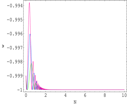
Figure 1: The evolution of the equation of state of a real scalar field in potential Eq.(34). The green, blue and pink curve correspond to the choice of the dimensionless parameter $\frac{\lambda\phi_{0}\sigma_{0}^{2}}{H_{0}}=2.0000,4.0000,6.0000$

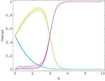
Figure 2: The evolution of cosmic density parameter of matter $\Omega_{M}$(green, yellow and orange curves), radiation $\Omega_{r}$ (blue curve) and dark energy $\Omega_{\phi}$ (pink, red and indigo curve) in potential Eq.(34). Since the parameters in the potential will not affect the shape of the plot significantly, we here plot for different initial $x$ and $y$, which affect the plot as shown in the figure.

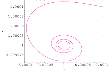
Figure 3: The attractor property of the system in the phase plane for the real scalar field model in potential Eq.(34)

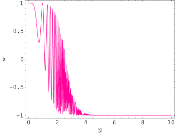
Figure 4: The evolution of the equation of state of scalar fields with O(N) internal symmetry in potential Eq.(34). The increase of oscillation is resulted from the introduction of the internal symmetry.

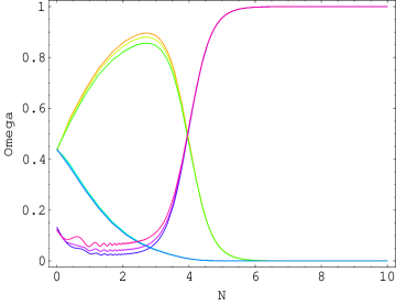
Figure 5: The evolution of cosmic density parameter of matter $\Omega_{M}$(green, yellow and orange curves), radiation $\Omega_{r}$ (blue curve) and O(N) scalar $\Omega_{\phi}$ (pink, red and indigo curve) in potential Eq.(34). Note that the term $\frac{\Sigma^{2}}{a^{6}\phi^{3}}$ resulted from the internal symmetry make the evolution quite different from that without internal symmetry at early epoch (the tilt of the yellow curve at the initial state). Similar as in Fig.2, we here plot for different initial $x$ and $y$, which affect the plot as shown in the figure.

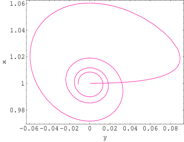
Figure 6: The attractor property of the system in the phase plane for the O(N) scalar field model in potential Eq.(34)

Figure 7: The evolution of the equation of state of phantom field in potential Eq.(34)

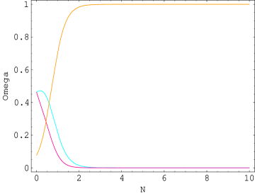
Figure 8: The evolution of cosmic density parameter of matter $\Omega_{M}$(blue curve), radiation $\Omega_{r}$ (red curve) and phantom $\Omega_{\phi}$ (yellow curve) in potential Eq.(34)

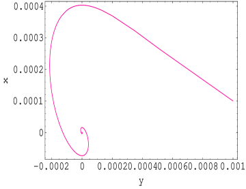
Figure 9: The attractor property of the dynamical system in the phase plane for the phantom model in potential Eq.(34)

One can also consider some other widely investigated potentials such as the exponential potential $V(\phi)=V_{0}\exp(-\lambda\kappa\phi)$ and inverse power potential $V(\phi)=V_{0}(\phi_{0}/\phi)^{q}$. It easily observes that these potentials admit vanishing minimum at $\phi\longrightarrow\infty$. The field will evolve towards the minimum of the potentials while can not reach them at finite time because the minimum corresponds to the infinite $\phi$, and therefore the existence of late time attractor solution for these types of potential need only the existence of minimum and the ”non-vanishing” condition is not necessarily held.

VII. Discussions

In this paper, we propose a way to construct viable dark energy models featured by a late time de Sitter attractor. We show that the dark energy model will admit a late time attractor solution if the potential of the scalar field with both canonical and Born-Infeld type Lagrangian has non-vanishing minimum. This condition becomes that the potential has non-vanishing maximum for the phantom models. When the field starts from the neighborhood of the maximum (minimum for the phantom models), it will be attracted to evolve towards the maximum/minimum, at which it will stay. This stable attractor regime corresponds to the equation of state $w_{\phi}=-1$ and cosmic density parameter $\Omega_{\phi}=1$, which do not contradict with current observations. The current observation data indicate that the cosmic density parameter of the dark energy is about $\Omega_{\phi}=2/3$ and the equation of state is less than $-0.82$Melchiorri , therefore, in the models analyzed in this paper, current universe is not at the attractor, instead, it is just on the way to the attractor. It is necessary to point out that the condition given in this paper for a viable dark energy model is only a sufficient condition and thus strictly speaking, it could not be used to rule out the possibility of the existence of late time attractor solution for a given potential. But it can tell us how to construct one.

ACKNOWLEDGEMENT: This work was partially supported by National Nature Science Foundation of China under Grant No. 19875016 and Foundation of Shanghai Development for Science and Technology under Grant No.01JC14035.

References

- (1) A. G. Riess et al. Astron. J. 116, 1009(1998)
- (2) S. Perlmutter et al. Astrophys. J. 517, 565(1999 )
- (3) J. L. Tonry et al., arXiv: astro-ph/0305008
- (4) C. L. Bennett et al., arXiv: astro-ph/0302207
- (5) C. B. Netterfield et al., astrophysics. J. 517, 604 (2002)
- (6) N. W. Halverson et al., Astrophysics. J. 568, 38 (2002)
- (7) B. Ratra and P. J. Peebles, Phys. Rev. D37 3406(1988)
- (8) K. Coble, S. Dodelson, J. Frieman, Phys. Rev. D55, 1851(1997)
- (9) R. R. Caldwell, R. Dave and P. J. Steinhardt, Phys. Rev. Lett. 80, 1582(1998)
- (10) P. J. E. Peebles, Bharat Ratra, Rev.Mod.Phys. 75, 599(2003); T. Padmanabhan, Phys. Rept. 380 235 (2003)
- (11) R.R. Caldwell, Phys.Lett. B545, 23(2002).
- (12) S. M. Carroll, M. Hoffman, M. Trodden, arXiv: astro-ph/0301273
- (13) P. H. Frampton, arXiv: hep-th/0302007
- (14) J. G. Hao and X. Z. Li, Phys. Rev. D67, 107303 (2003)
- (15) X. Z. Li and J. G. Hao, arXiv: hep-th/0303093
- (16) G. W. Gibbons, arXiv: hep-th/0302199
- (17) A. Feinstein and S. Jhingan, arXiv: hep-th/0304069; L. P. Chimento and A. Feinstein, arXiv: astro-ph/0305007
- (18) P. Singh, M.Sami and N. Dadhich, arXiv: hep-th/0305110
- (19) P. J. Steinhardt, L. Wang, I. Zlatev, Phys.Rev. D59, 123504 (1999); E. J. Copeland, A. R. Liddle and D. Wands,Phys.Rev. D57, 4686 (1998); S. C. C. Ng, N. J. Nunes, F. Rosati,Phys.Rev. D64, 083510(2001)
- (20) A. Melchiorri, L. Mersini, C. J. Odman and M. Trodden, arXiv: astro-ph/0211522
- (21) R. R Caldwell, M. Kamionkowski and N. N. Weinberg, astro-ph/0302506
- (22) B. McInnes, JHEP 0208 029 (2002)
- (23) J. A. Gu and W. Y. Huang, Phys.Lett. B517 1 (2001)
- (24) L. A. Boyle, R. R. Caldwell and M. Kamionkowski, Phys.Lett. B545 17 (2002).
- (25) X. Z. Li, J. G. Hao and D. J. Liu, Class.Quant.Grav. 19 6049 (2002)
- (26) A. Sen, JHEP 0204, 048 (2002); A. Sen, JHEP 0207, 065(2002);
- (27) G.W.Gibbons, Phys. Lett. B537, 1 (2002); M. Fairbairn and M. H. G. Tytgat, Phys.Lett.B546, 1 (2002); T. Padmanabhan, Phys. Rev. D66 021301 (2002); A. Feinstein, Phys. Rev. D66 063511 (2002); X. Z. Li and X. H. Zhai, Phys. Rev.D67, 067501(2003); M. Sami and T. Padmanabhan, Phys. Rev. D67, 083509(2003); L. Kofman and A. Linde, JHEP 0207 004 (2002); X. Z. Li, D. J. Liu and J. G. Hao, arXiv: hep-th/0207146; M. Sami, P. Chingangbam and T. Qureshi, Phys.Rev. D66 043530(2002);
- (28) J. G. Hao and X. Z. Li, Phys. Rev. D66, 087301(2002); X. Z. Li, J. G. Hao and D. J. Liu, Chin.Phys.Lett.19 1584 (2002); J. S. Bagla, H. K. Jassal and T. Padmanabhan, Phys.Rev. D67, 063504 (2003);
- (29) J. G. Hao and X. Z. Li, arXiv: hep-th/0305207, to be published in Phys. Rev. D