Signatures in the Planck Regime

Abstract

String theory suggests the existence of a minimum length scale. An exciting quantum mechanical implication of this feature is a modification of the uncertainty principle. In contrast to the conventional approach, this generalised uncertainty principle does not allow to resolve space time distances below the Planck length. In models with extra dimensions, which are also motivated by string theory, the Planck scale can be lowered to values accessible by ultra high energetic cosmic rays (UHECRs) and by future colliders, i.e. $M_{f}\approx$ 1 TeV. It is demonstrated that in this novel scenario, short distance physics below $1/M_{f}$ is completely cloaked by the uncertainty principle. Therefore, Planckian effects could be the final physics discovery at future colliders and in UHECRs. As an application, we predict the modifications to the $e^{+}e^{-}\to f^{+}f^{-}$ cross-sections.

I Introduction

Even if a full description of quantum gravity is not yet available, there are some general features that seem to go hand in hand with all promising candidates for such a theory. One of them is the need for a higher dimensional space-time, one other the existence of a minimal length scale. The scale at which the running couplings unify and quantum gravity is likely to occur is called the Planck scale. At this scale the quantum effects of gravitation get as important as those of the electroweak and strong interactions.

In this paper we will implement both of these extensions in the standard model without the aim to derive them from a fully consistent theory. Instead, we will to analyse some of the main features that may arise by the assumptions of extra dimensions and a minimal length scale.

In perturbative string theory [1, 2], the feature of a fundamental minimal length scale arises from the fact that strings can not probe distances smaller than the string scale. If the energy of a string reaches the Planck mass $m_{\rm p}$, excitations of the string can occur and cause a non-zero extension [3]. Due to this, uncertainty in position measurement can never become smaller than $l_{\rm p}=\hbar/m_{\rm p}$. For a review, see [4, 5].

Naturally, this minimum length uncertainty is related to a modification of the standard commutation relations between position and momentum [6, 7]. Application of this is of high interest for quantum fluctuations in the early universe and for inflation [8, 9, 10, 11, 12, 13, 14, 15, 16].

The incorporation of the modified commutation relations into quantum theory is not fully consistent in all approaches, therefore we will define physical variables step by step.

The existence of a minimal length scale becomes important even for collider physics with the further incorporation of the central idea of Large eXtra Dimensions (LXDs). The model of LXDs, which was recently proposed in [17, 18, 19, 20, 21], might allow to study interactions at Planckian energies in the next generation collider experiments. Here, the hierarchy-problem is solved or at least reformulated in a geometric language by the existence of $d$ compactified LXDs in which only the gravitons can propagate. The standard model particles are bound to our 4-dimensional sub-manifold, often called our 3-brane. This results in a lowering of the Planck scale to a new fundamental scale, $M_{f}$, and gives rise to the exciting possibility of TeV scale GUTs [22].

The strength of a force at a distance $r$ generated by a charge depends on the number of space-like dimensions. For distances smaller than the compactification radius $R$, the gravitational interaction drops faster compared to the other interactions. For distances much bigger than $R$, gravity is described by the well known potential law $\propto 1/r$. However, for $r\leq R$ the force lines are diluted into the extra dimensions. Assuming a smooth transition to Newton’s law, this results in a smaller effective coupling constant for gravity.

This leads to the following relation between the four-dimensional Planck mass $m_{\rm p}$ and the higher dimensional Planck mass $M_{f}$, which is the new fundamental scale of the theory:

$$m_{\rm p}^{2}=R^{d}M_{f}^{d+2}\quad.$$ (1)

The lowered fundamental scale would lead to a vast number of observable phenomena for quantum gravity at energies in the range $M_{f}$. In fact, the non-observation of these predicted features gives first constraints on the parameters of the model, the number of extra dimensions $d$ and the fundamental scale $M_{f}$ [23, 24, 25]. On the one hand, this scenario has major consequences for cosmology and astrophysics such as the modification of inflation in the early universe and enhanced supernova-cooling due to graviton emission [19, 26, 27, 28, 29]. On the other hand, additional processes are expected in high-energy collisions [30]: production of real and virtual gravitons [31, 32, 33, 34, 35] and the creation of black holes at energies that can be achieved at colliders in the near future [36, 37, 38, 39, 40, 41, 42] and in ultra high energetic cosmic rays [43, 44].

This paper is organised as follows. We will begin with a sketch of the basics of quantum mechanics (section II), and in the third section modify these familiar relations by introducing generalised uncertainty. This will be done in $1+1$ dimensions first, then we care for the full $3+1$ dimensional description (this is understood to be the analysis on our brane). To examine the phenomenological implications on a basic level, we first analyse the modified Schrödinger Equation, the Dirac Equation and the Klein-Gordon Equation in sections IV-VI. In section VII we investigate the influence of the minimal length scale on QED cross-sections at tree-level and compare with $e^{+}e^{-}$ data. Section VIII provides an estimation of the effect on graviton production. We end with a conclusion of our results in section IX.

In the following, we use the convention $\hbar=L_{f}M_{f}$, $c=1$. Greek indices $\alpha,\mu,...$ run from 0 to 3. Latin indices $i,j,...$ run from 1 to 3, latin indices $a,b,...$ run from 4 to $4+d$. In order to distinguish the ordinary quantities (e.g. $E$) from the modified ones, we label the latter with a tilde ($\tilde{E}$).

II The Uncertainty Relation

In standard quantum mechanics translations in space and time are generated by momentum $p_{i}$ and energy $E$, respectively. However, from purely dimensional reasons, the generators of the translations in space and time are the wave vector $k_{i}$ and the frequency $\omega$. The relation between $(k_{i},\omega)$ and $(p_{i},E)$ is usually given, of course, by the constant $\hbar$ (often chosen to be equal one):

$$p_{i} = \hbar k_{i}\quad,$$ (2)

$$E = \hbar\omega\quad.$$ (3)

In the present context it is of utmost importance to re-investigate this relation carefully.

Using the well known commutation relations

$$[\hat{x}_{i},\hat{k}_{j}]={\mathrm{i}}\delta_{ij}\quad,$$ (4)

quantisation in position representation $\hat{x}_{i}=x_{i}$ leads to:

$$\hat{k}_{i}=-{\mathrm{i}}\partial_{i}\quad \quad\hat{p}_{i}=\hbar\hat{k}_{i}=-{\mathrm{i}}\hbar\partial_{i}\quad,$$ , (5)

$$\hat{\omega}=+{\mathrm{i}}\partial_{t}\quad \quad\hat{E}=\hbar\hat{\omega}\;=+{\mathrm{i}}\hbar\partial_{t}\quad.$$ , (6)

In the momentum representation, $\hat{p}_{i}=p_{i}$, the commutation relation is fulfilled by

$$\hat{x}_{i}={\mathrm{i}}\hbar\frac{\partial}{\partial p_{i}}={\mathrm{i}}\frac{\partial p_{i}}{\partial k_{i}}\frac{\partial}{\partial p_{i}}={\mathrm{i}}\frac{\partial}{\partial k_{i}}\quad.$$ (7)

The general relation for the root mean square deviations for the expectation values of two operators $\hat{A}$ and $\hat{B}$,

$$\Delta A\Delta B\geq\frac{1}{2}\left|\langle[\hat{A},\hat{B}]\rangle\right|\quad,$$ (8)

then leads to the uncertainty relation

$$\Delta p_{i}\Delta x_{i}\geq\frac{1}{2}\hbar\quad.$$ (9)

The equation of motion (no explicit time dependence) for the wave function is generated by the evolution operator $\hat{U}$:

$$|\psi(t)\rangle = \hat{U}(t-t_{o})|\psi(t_{o})\rangle\quad,$$ (10)

$$\hat{U}(t-t_{o}) = \exp\left(-\frac{{\rm i}}{\hbar}\hat{E}(t-t_{o})\right)\quad,$$ (11)

$$\Rightarrow\quad+{\rm i}\hbar\partial_{t}|\psi\rangle = \hat{E}|\psi\rangle\quad.$$ (12)

The time dependence of an operator $\hat{A}$ (no explicit time dependence) is (in the Heisenberg picture) then given by

$$\frac{{\rm d}}{{\rm d}t}\hat{A}=[\hat{A},\hat{E}]\quad.$$ (13)

III Generalised Uncertainty

In order to implement the notion of a minimal length $L_{f}$, let us now suppose that one can increase $p$ arbitrarily, but that $k$ has an upper bound. This effect will show up when $p$ approaches a certain scale $M_{f}$. The physical interpretation of this is that particles could not possess arbitrarily small Compton wavelengths $\lambda=2\pi/k$ and that arbitrarily small scales could not be resolved anymore.

To incorporate this behaviour, we assume a relation $k=k(p)$ between $p$ and $k$ which is an uneven function (because of parity) and which asymptotically approaches $1/L_{f}$. Furthermore, we demand the functional relation between the energy $E$ and the frequency $\omega$ to be the same as that between the wave vector $k$ and the momentum $p$.

In contrast to [8], there is no modified dispersion relation in our approach, since $\partial\omega/\partial k=\partial E/\partial p$. This means that the functional behaviour of $k(p)$ is the same as that of $\omega(E)$ up to a constant. A possible choice for these relations is

$$L_{f}k(p) = \tanh^{1/\gamma}\left[\left(\frac{p}{M_{f}}\right)^{\gamma}\right]\quad,$$ (14)

$$L_{f}\omega(E) = \tanh^{1/\gamma}\left[\left(\frac{E}{M_{f}}\right)^{\gamma}\right]\quad,$$ (15)

with a real, positive constant $\gamma$. For simplicity, we will use $\gamma=1$.

In the following we will study two approximations, from here on referred to as cases (a) and (b):

• The regime of first effects including order $(p/M_{f})^{3}$ contributions and

• The high energy limit $p\gg M_{f}$.

Expanding $\tanh(x)$ for small arguments gives for case (a)

$$L_{f}k(p) \approx \frac{p}{M_{f}}-\frac{1}{3}\left(\frac{p}{M_{f}}\right)^{3}$$ (16)

$$L_{f}\omega(E) \approx \frac{E}{M_{f}}-\frac{1}{3}\left(\frac{E}{M_{f}}\right)^{3}$$ (17)

$$\frac{1}{M_{f}}p(k) \approx kL_{f}+\frac{1}{3}\left(kL_{f}\right)^{3}$$ (18)

$$\frac{1}{M_{f}}E(\omega) \approx \omega L_{f}+\frac{1}{3}\left(\omega L_{f}\right)^{3}\quad.$$ (19)

This yields to 3^rd order

$$\hbar\frac{\partial k}{\partial p} \approx 1-\left(\frac{p}{M_{f}}\right)^{2}$$ (20)

$$\approx 1-\left(kL_{f}\right)^{2}$$ (21)

$$\frac{1}{\hbar}\frac{\partial p}{\partial k} \approx 1+\left(kL_{f}\right)^{2}$$ (22)

$$\approx 1+\left(\frac{p}{M_{f}}\right)^{2}\quad.$$ (23)

In case (b) we have $\tanh(x)\approx\pm 1\mp 2\exp(\mp 2x)$ for $|x|\gg 1$, with the upper signs for positive values of $x$. Skipping one factor $2$ in the exponent, which can be absorbed by a redefinition of $M_{f}$, one obtains:

$$L_{f}k(p) \approx \pm 1\mp 2\exp\left(\mp\frac{p}{M_{f}}\right)$$ (24)

$$L_{f}\omega(E) \approx \pm 1\mp 2\exp\left(\mp\frac{E}{M_{f}}\right)$$ (25)

$$\frac{1}{M_{f}}p(k) \approx \mp\ln\left(\frac{1\mp kL_{f}}{2}\right)$$ (26)

$$\frac{1}{M_{f}}E(\omega) \approx \mp\ln\left(\frac{1\mp\omega L_{f}}{2}\right)\quad.$$ (27)

The derivatives are

$$\hbar\frac{\partial k}{\partial p} \approx 2\exp\left(-\frac{|p|}{M_{f}}\right)$$ (28)

$$\frac{1}{\hbar}\frac{\partial p}{\partial k} \approx \frac{1}{2}\frac{1}{1\mp kL_{f}}\;.$$ (29)

The quantisation of these relations is straight forward. The commutators between $\hat{k}$ and $\hat{x}$ remain in the standard form given by Eq. (4). Inserting the functional relation between the wave vector and the momentum then yields the modified commutator for the momentum. With the commutator relation

$$[\,\hat{x},\hat{A}(k)]=+{\rm i}\frac{\partial A}{\partial k}\quad,$$ (30)

the modified commutator algebra now reads

$$[\,\hat{x},\hat{p}] = +{\rm i}\frac{\partial p}{\partial k}\quad.$$ (31)

This results in the generalised uncertainty relation

$$\Delta p\Delta x\geq\frac{1}{2}\Bigg{|}\left\langle\frac{\partial p}{\partial k}\right\rangle\Bigg{|}\quad.$$ (32)

In case (a), with the approximations (16)-(19), the results of Ref. [8] are reproduced:

$$[\hat{x},\hat{p}] \approx {\rm i}\hbar\left(1+\frac{\hat{p}^{2}}{M_{f}^{2}}\right)$$ (33)

giving the generalised uncertainty relation

$$\Delta p\Delta x\geq\frac{1}{2}\hbar\left(1+\frac{\langle\hat{p}^{2}\rangle}{M_{f}^{2}}\right)\quad.$$ (34)

In the asymptotic case (b) this yields

$$[\,\hat{x},\hat{p}] \approx {\rm i}\frac{\hbar}{2}\,\exp\left(+\frac{|\hat{p}|}{M_{f}}\right)\quad,$$ (35)

$$\Delta p\Delta x \geq \frac{1}{4}\hbar\,\left\langle\exp\left(+\frac{|\hat{p}|}{M_{f}}\right)\right\rangle\quad.$$ (36)

Quantisation proceeds in the usual way from the commutation relations. For scattering theory it is convenient to work in the momentum representation, $\hat{p}=p,\hat{k}=k(p)$. From Eq. 7,

$$\hat{x} = {\rm i}\partial_{k}={\rm i}\frac{\partial p}{\partial k}\partial_{p}$$ (37)

we obtain in case (a) (first derived in Ref. [6]):

$$\hat{x} \approx {\rm i}\hbar\left(1+\frac{p^{2}}{M_{f}^{2}}\right)\partial_{p}\quad,$$ (38)

and in case (b):

$$\hat{x} \approx {\rm i}\frac{\hbar}{2}\,\exp\left(\frac{|p|}{M_{f}}\right)\partial_{p}$$ (39)

As a first application of this approach to quantum mechanics, we will study the Schrödinger Equation in section IV. Focusing on conservative potentials in non relativistic quantum mechanics we give the operators in the position representation which is suited best for this purpose:

$$\hat{x} = x\quad,\quad\hat{k}=-{\rm i}\partial_{x}$$ (40)

$$\hat{p} = \hat{p}(\hat{k})\quad,$$ (41)

yielding in case (a)

$$\hat{p} \approx -{\rm i}\hbar\left(1-\frac{L_{f}^{2}}{3}\partial_{x}^{2}\right)\partial_{x}\quad.$$ (42)

The new momentum operator now includes higher derivatives.

Since $k=k(p)$ we have $\hat{p}(\hat{k})|k\rangle=p(k)|k\rangle$ and so $|k\rangle\propto|p(k)\rangle$. We could now add that both sets of eigenvectors have to be a complete orthonormal system and therefore $\langle k^{\prime}|k\rangle=\delta(k-k^{\prime})$, $\langle p^{\prime}|p\rangle=\delta(p-p^{\prime})$. This seems to be a reasonable choice at first sight, since $|k\rangle$ is known from the cis-Planckian regime. Unfortunately, now the normalisation of the states is different because $k$ is restricted to the Brillouin zone $-1/L_{f}$ to $1/L_{f}$.

To avoid the need to recalculate normalisation factors, we choose the $|p(k)\rangle$ to be identical to the $|k\rangle$. Following the proposal of [6] this yields

$$\langle p^{\prime}|p\rangle = \langle k(p)|k(p^{\prime})\rangle=\delta\left(k(p)-k(p^{\prime})\right)$$ (43)

$$= \frac{\partial p}{\partial k}\delta\left(p-p^{\prime}\right)$$ (44)

and avoids a new normalisation of the eigen functions by a redefinition of the measure in momentum space

$${\mathrm{d}}p\rightarrow\frac{{\mathrm{d}}p}{\hbar}\frac{\partial k}{\partial p}\quad.$$ (45)

This redefinition has a physical interpretation because we expect the momentum space to be squeezed at high momentum values and weighted less.

For the different cases under discussion, one gets:
Case (a):

$$\frac{{\mathrm{d}}p}{\hbar}\rightarrow\frac{{\mathrm{d}}p}{\hbar}\frac{1}{1+(p/M_{f})^{2}}\quad.$$ (46)

Case (b):

$$\frac{{\mathrm{d}}p}{\hbar}\rightarrow\frac{{\mathrm{d}}p}{\hbar}\,2\exp\left(-\frac{|p|}{M_{f}}\right)\quad.$$ (47)

The operator of time translation is no longer identical to the energy operator times $\hbar$ in this context. In ordinary quantum mechanics, both of them are $\propto\hat{H}$. To avoid confusion, let $\hat{\omega}$ be that operator defined by the generator of the Lorentz-Algebra which belongs to the time translation and $\hat{E}=\hat{E}(\hat{\omega})$ the energy-operator for the free particle. $\hat{E}_{{\rm tot}}=\hat{E}(\hat{\omega})+V(\hat{x})$ is then the operator of the total energy, including a time-independent potential $V(x)$. The equation of motion for the wave function is then given by

$$\hat{U}(t-t_{o}) = \exp\left(-{\rm i}\hat{\omega}(\hat{E}_{{\rm tot}})(t-t_{o})\right)\quad,$$ (48)

$$\Rightarrow\quad{\rm i}\partial_{t}|\psi\rangle = \hat{\omega}(\hat{E}_{{\rm tot}})|\psi\rangle\quad,$$ (49)

which has in case (a) the explicit form

$${\rm i}\hbar\partial_{t}|\psi\rangle \approx +\left(\hat{E}_{{\rm tot}}-\hat{E}_{{\rm tot}}^{3}/3M_{f}^{2}\right)|\psi\rangle\quad.$$ (50)

A Lorentz Invariance and Conservation Laws in Four Dimensions

We will use the following short notations:

$$k = |\vec{k}|\quad,\quad\vec{k}=(k_{x},k_{y},k_{z})\quad,\quad{\underline{\bf k}}=(\vec{k},\omega)\quad,$$ (51)

$$p = |\vec{p}|\quad,\quad\vec{p}=(p_{x},p_{y},p_{z})\quad,\quad{\underline{\bf p}}=(\vec{p},E)\quad.$$ (52)

As discussed above, we leave the dispersion relation unmodified. However, as $E=\sqrt{p^{2}+m^{2}}$ expresses the relativistic energy-momentum relation we meet a serious problem at this point. The mass-shell relation is a consequence of ${\underline{\bf p}}$ being a Lorentz vector rather than ${\underline{\bf k}}$. Thus, we have to reconsider Lorentz covariance in the trans Planckian regime. For energy scales below $M_{f}$, an observer boosted to high velocities would observe arbitrarily large energies. We have to assure then, that the Lorentz-transformed ${\underline{\bf k}}$ always stays below the new limit, which means its transformation properties are not identical to those of the momentum ${\underline{\bf p}}$. To put this in other words, a Lorentz boosted observer is not allowed to see the minimal length further contracted. Several proposals have been made to solve this problem. Most of them suggest a modification of the Lorentz transformation [45, 46, 47, 48], but the treatment is still under debate.

However, the appearance of this problem might not be as astonishing as it seems at first sight. Because the modifications we examine do occur at energies at which quantum gravity will get important, curvature corrections to the space time must not be neglected anymore. Therefore, the quantities should be general relativistic covariant rather than flat space Lorentz covariant. These effects will then exhibit themselves in strong background fields, but here also the particle’s curvature itself makes an essential contribution. The exact – but unknown – transformation should assure that no coordinate transformation can push ${\underline{\bf k}}$ beyond the Planck scale. For practical use of the modified quantum theory considered here, we treat the momentum ${\underline{\bf p}}$ as the Lorentz covariant partner of the wave vector ${\underline{\bf k}}$. We will assume that the momentum is Lorentz covariant and that the functional relation between the two quantities, although unknown, is of the desired behaviour. Inserting one of the approximations at the end of the computation then breaks Lorentz covariance.

In fact, in the present scenario ${\underline{\bf k}}$ is also not a conserved quantity in interactions, because the relation between ${\underline{\bf p}}$ and ${\underline{\bf k}}$ is not linear anymore. In single particle dynamics we have ,in generalisation of Eq. (13), the time evolution of the operator $\hat{A}$

$$\frac{{\rm d}}{{\rm d}t}\hat{A}=[\hat{A},\hat{\omega}]$$ (53)

Since $[\hat{A},\hat{B}]=0$ is equivalent to $[\hat{A},f(\hat{B})]=0$ for any well defined functions $f$ of $\hat{B}$, quantities conserved in ordinary quantum mechanics are also conserved in the approach considered here. In particular, the single particle momentum $\hat{p}$ and energy $\hat{E}$ are conserved if no interactions occur.

The canonical commutation relations are given by

$$[\,x^{\nu},p_{\mu}] = +{\rm i}\frac{\partial p_{\mu}}{\partial k_{\nu}}\quad,$$ (54)

and

$$[p_{\nu},p_{\mu}]=0\quad,$$ (55)

with ${\underline{\bf p}}={\underline{\bf p}}({\underline{\bf k}})$ being a Lorentz vector and fulfilling all requirements mentioned above.

The invariant volume element is then modified to be

$${\mathrm{d}}^{4}p \rightarrow \frac{{\mathrm{d}}^{4}p}{\hbar^{4}}\;{\rm det}\left(\frac{\partial k_{\mu}}{\partial p_{\nu}}\right)$$ (56)

$$= \frac{{\mathrm{d}}^{4}p}{\hbar^{4}}\prod_{\nu}\frac{\partial k_{\nu}}{\partial p_{\nu}}\quad.$$ (57)

In the last step we used the rotational invariance of the relations $p_{\mu}=p_{\mu}(k_{\mu})$. Due to this the Jacobi matrix is diagonal.

B The Non-Relativistic Case: Three Dimensions

This generalises our $1+1$-dimensional treatment from the first section. Note that this approach is no longer Lorentz invariant and therefore suited for non-relativistic scenarios only.

$$[\,\hat{x}_{i},\hat{p}_{j}] = {\rm i}\hbar\delta_{ij}\frac{\partial p_{i}}{\partial k_{j}}\quad,$$ (58)

$${}[\hat{p}_{i},\hat{p}_{j}] = 0\quad.$$ (59)

Rotational invariance implies for case (a)

$$[\hat{x}_{i},\hat{p}_{j}] = {\rm i}\hbar\delta_{ij}\left(1+\frac{\hat{p}^{\;2}}{M_{f}^{2}}\right)\quad,$$ (60)

$${}[\hat{p}^{i},\hat{p}_{j}] = 0\quad.$$ (61)

In the position representation $\vec{\nabla}=(\partial_{x},\partial_{y},\partial_{z})$ the momentum operator then reads

$$\hat{\vec{p}}=-{\rm i}\hbar\vec{\nabla}\left(1-\frac{L_{f}^{2}}{3}\vec{\nabla}^{\;2}\right)$$ (62)

IV Schrödinger Equation

First we will have a look at the free scalar particle in the low energy limit. We will define physical variables step by step since different approaches to incorporate the minimal length into quantum theory have been given in the literature.

Let us consider the modified Schrödinger equation. For usual one gets it by quantising the low energy expansion, $p/m\ll 1$, of the relativistic expression

$$E=m\sqrt{1+\frac{p^{2}}{m^{2}}}=m\left(1+\frac{p^{2}}{2m^{2}}+{\cal{O}}((p/m)^{3})\right)$$ (63)

and dropping the constant term $m$ because an additive constant in the Hamiltonian does not change the dynamics. By multiplying a phase $\exp(-{\rm i}mt)$ to $|\psi\rangle$ we could get rid of it. But now this prescription is not applicable anymore because an additive constant in $E$ does not yield an additive constant in $\omega$ and therefore is has to be kept.

With

$$E^{3}=m^{3}\left(1+\frac{3p^{2}}{2m^{2}}+{\cal{O}}((p/m)^{3})\right)$$ (64)

the modified Schrödinger Equation, see (49), is then given by

$${\rm i}\hbar\;\partial_{t}|\psi\rangle = \left[m\left(1-\frac{m^{2}}{3M_{f}^{2}}\right)+\frac{\hat{p}^{2}}{2m}\left(1-\frac{m^{2}}{M_{f}^{2}}\right)\right]|\psi\rangle\quad.$$ (65)

The first term can be dropped again, since it contributes only an overall phase factor. This means, that up to order $p^{2}/M_{f}^{2}$ and $p^{2}/m^{2}$ no change in the dynamics occurs. However, the kept term $m$ will yield extra terms in higher order approximations. Equation (65) will modify the frequency spectrum of very heavy ($m\approx M_{f}$) non relativistic particles and has therefore little applications.

Fortunately, we are mainly interested in general in the energy spectrum and do not need to calculate $\hat{\omega}$ at all. Let us proceed now with the Schrödinger equation for a particle in a potential $V(\hat{x})$ with the two most prominent cases: the harmonic oscillator and the hydrogen atom. We want to calculate the modified energy levels $\tilde{E}_{n}$ as solutions of the time-independent Schrödinger equation. In the following we add $m\ll M_{f}$. The time dependence is split off by a separation of the variables and has the form $\exp(-{\rm i}\omega_{n}t)$ with $\omega_{n}=\omega(\tilde{E}_{n})$.

$$\tilde{E}_{n}|\psi\rangle = \left(\frac{\hat{p}^{2}}{2m}+V(\hat{x})\right)|\psi\rangle\quad.$$ (66)

For the harmonic oscillator with $V(x)=m\Omega^{2}x^{2}/2$ in the momentum representation, we find using Eq. (38)

$$\tilde{E}_{n}|\psi\rangle = \left(\frac{p^{2}}{2m}-\frac{m\hbar^{2}\Omega^{2}}{2}\left((1+p^{2}/M_{f}^{2})\partial_{p}\right)^{2}\right)|\psi\rangle\quad.$$ (67)

An analytic solution of this differential equation has been given in [6] and, for a more general setting, in [49].

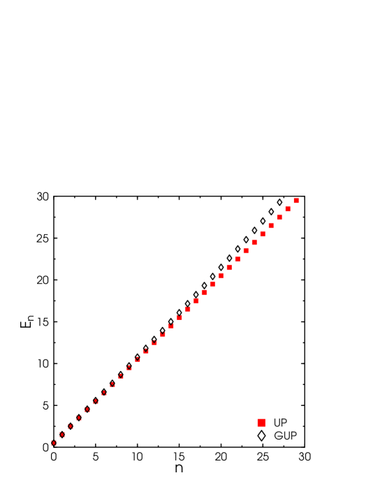
FIG. 1.: The energy levels of the harmonic oscillator with usual uncertainty (UP) in comparison to the case with generalised uncertainty (GUP). Here, $\Omega=m=1,M_{f}=0.1$.

The momentum space equation (67) is well suited for a numerical treatment. We have solved this eigenvalue problem numerically and it fits the analytically obtained values of [6] to very high precision. This is plotted in Fig. 1 for $\Omega=m=1$ and $M_{f}=0.1$. It can be seen qualitatively that the levels get shifted to higher energies with increasing $n$ in comparison to the usual $E_{n}\propto 1/2+n$. If one tries to solve the eigenvalue equation in the position representation,

$$\tilde{E}_{n}|\psi\rangle = -\frac{\hbar^{2}}{2m}\left[\left(1-\frac{L_{f}^{2}}{3}\partial^{2}_{x}\right)\,\partial_{x}\right]^{2}+\frac{m\omega^{2}}{2}x^{2}|\psi\rangle\quad,$$ (68)

one has to cope with the higher derivatives, and adequate numerical methods to treat this stiff problem properly are quite involved. However, for practical purposes, one can consider the higher order terms as perturbations to the standard quantum mechanics problem and resort to perturbation theory, as was done analytically for the three dimensional harmonic oscillator in [50]. Our perturbative calculations have shown numerically, that first order perturbation theory reaches 5 percent of the exact eigenvalues of the harmonic oscillator in the GUP regime.

The hydrogen atom is treated best in position representation to avoid the problem of substituting $\hat{x}={\rm i}\partial_{k}$ in the $1/r$ potential. To derive the equation for the Coulomb potential $V(r)=e^{2}/r$ we will as usual first transform into spherical coordinates $r,\theta,\phi$ with $r=|\vec{r}|$. We look only at the case of vanishing angular dependence, $l=0$. (For a treatment of the full angular dependence see [51], who uses the perturbation theory method to calculate the shift in the energy spectrum). We have then in position representation

$$\hat{p}_{r}={\rm i}\hbar\frac{1}{r}\partial_{r}\left(1-\frac{L_{f}^{2}}{3}\partial^{2}_{r}\right)r\quad,$$ (69)

and for the energy operator we find

$$\hat{E} = -\frac{\hbar^{2}}{2mr}\left(\partial_{r}-\frac{L_{f}^{2}}{3}\partial^{3}_{r}\right)^{2}r+\frac{e^{2}}{r}\quad.$$ (70)

For the calculation of the eigenvalues $\tilde{E}_{n}$ of $\hat{E}$ we can substitute as usual $|\phi\rangle=r|\psi\rangle$ and then deal with the equation

$$\tilde{E}_{n}|\phi\rangle = \left(-\frac{\hbar^{2}}{2m}\left(\partial_{r}-\frac{L_{f}^{2}}{3}\partial^{3}_{r}\right)^{2}+\frac{e^{2}}{r}\right)|\phi\rangle\quad.$$ (71)

As in the case of the harmonic oscillator, the higher derivatives can be treated as perturbations, and the corresponding shifts of the energy levels can be calculated.

There is, however, a second way to calculate the energy levels, which applies the semi classical calculation of Bohr to the generalised uncertainty principle.

The Coulomb potential is a central potential, hence the virial theorem states that for a particle moving in this potential, $E_{\rm kin}=-\frac{1}{2}E_{{\rm pot}}$. For an electron of mass $m_{\rm e}$ in the $n$-th level, the total energy $E_{n}$ is

$$E_{n}=E^{{\rm kin}}_{n}+E^{{\rm pot}}_{n}=\frac{1}{2}E^{{\rm pot}}_{n}=-E^{{\rm kin}}_{n}\quad.$$ (72)

Adding the Bohr quantisation condition, the wavelength of the electron fits the circumference of the orbit, one finds for the $n$th level $\lambda=2\pi nR_{n}$, hence $k(p)=n/R_{n}$. Now $E_{n}=\frac{1}{2}e^{2}/R_{n}$, so the modified $n$-th energy level $\tilde{E}_{n}$ of the hydrogen atom fulfils

$$\tilde{E}_{n}^{2} = \frac{e^{4}}{4}\frac{1}{R_{n}^{2}}=\frac{e^{4}}{4}\frac{k(p)^{2}}{n^{2}}$$ (73)

Inserting now the approximation from eq. (16) for $k(p)$, we obtain

$$\tilde{E}_{n}^{2} = \frac{e^{4}}{4n^{2}\hbar^{2}}\,p^{2}\left(1-\frac{1}{3}\frac{p^{2}}{M_{f}^{2}}\right)^{2}\quad.$$ (74)

Since $\tilde{E}_{n}=-\tilde{E}^{{\rm kin}}_{n}=-p^{2}/2m_{\rm e}$, we can express $p^{2}$ by $\tilde{E}_{n}$, which results in the equation

$$\tilde{E}_{n}^{2} = -\frac{E_{0}}{n^{2}}\tilde{E}_{n}\left(1+\frac{4}{3}\frac{m_{\rm e}\tilde{E}_{n}}{M_{f}^{2}}+\frac{4}{9}\frac{m_{\rm e}^{2}\tilde{E}_{n}^{2}}{M_{f}^{4}}\right)\quad,$$ (75)

where

$$E_{0}=\frac{1}{2}\frac{e^{4}m_{\rm e}}{\hbar^{2}}\approx 13.6\,{\rm eV}$$ (76)

is the Rydberg constant. Introducing the abbreviations

$$\epsilon_{n}=\frac{E_{0}}{n^{2}}\,,\quad\quad\beta=\frac{m_{\rm e}}{3M_{f}^{2}}\quad,$$ (77)

the cubic equation for $\tilde{E}_{n}$ reads

$$\tilde{E}_{n}^{2}=-\epsilon_{n}\tilde{E}_{n}-4\epsilon_{n}\beta\tilde{E}_{n}^{2}-4\epsilon_{n}\beta^{2}\tilde{E}_{n}^{3}$$ (78)

which is solved by

$$\tilde{E}_{n} = \frac{1}{8}\frac{1}{\epsilon_{n}\beta^{2}}\left(\sqrt{1+8\epsilon_{n}\beta}-1-4\epsilon_{n}\beta\right)\quad$$ (79)

$$= \frac{9}{8}\frac{n^{2}M_{f}^{4}}{E_{0}m_{\rm e}^{2}}\left(\sqrt{1+\frac{8}{3}\frac{E_{0}m_{\rm e}}{n^{2}M_{f}^{2}}}-1-\frac{4}{3}\frac{E_{0}m_{\rm e}}{n^{2}M_{f}^{2}}\right)\quad.$$ (80)

Neglecting terms of order $O(1/M_{f}^{4})=O(\beta^{2})$, an expansion of the square root yields for the energy levels the expression

$$\tilde{E}_{n}\approx\,-\,\frac{E_{0}}{n^{2}}\left(1-\frac{4}{3}\frac{m}{M_{f}^{2}}\frac{E_{0}}{n^{2}}\right)\quad.$$ (81)

This results fits quite well at higher $n$ to numerical calculations from a perturbative treatment of the Hamiltonian we have done. Results are shown in Fig. 2.

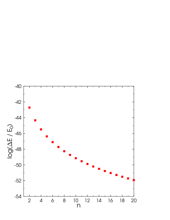
FIG. 2.: The difference of energy levels $\Delta E=\tilde{E}_{n}-E_{n}$ with $l=0$ in the Coulomb potential with usual uncertainty $\tilde{E}_{n}$ to the energy with generalised uncertainty $E_{n}$. Here, $M_{f}=1$TeV, $E_{0}=13.6$eV is the Rydberg constant.

We can now compare our result with that obtained in [51] from perturbation theory. In that paper it was found that with the modified uncertainty principle, the angular momentum degeneracy of the energy levels of the hydrogen atom is lifted. We expect the best match with our semi classical result for the energy levels of highest angular momentum for a given main quantum number $n$. In fact, for $l=n-1$, the results of [51] exhibit the same dependence of the shift on $E_{0}/n^{2}$ in the order $O(1/M_{f}^{2})$ for large $n$, differing by a factor $1/3$ from our values. We note that the shift found in [52] is similar in size, but has a different sign. All three results, however, are consistent enough in the absolute value of the shift in the energy levels to make comparisons to experimental data. As one might have expected, the deviation caused by the modified uncertainty principle is of order $E_{0}m_{e}/M_{f}^{2}$, and the $n$ dependence of the shift is the same in all three results.

To get a connection to experiment, we note that the transition frequency of the hydrogen atom from S1 to S2 level has been measured up to an accuracy of $1.8\times 10^{-14}$ [53]. In the frequency range of interest, we can certainly neglect transforming the energy into a frequency with the new formula. Inserting the values and the current accuracy yields $M_{f}\approx>50$ GeV, as was obtained by [52]. The dependence of relative energy level shift on the fundamental scale $M_{f}$ is shown in Fig. 3, together with the current experimental bound. An increase of the experimental precision by four orders of magnitude would allow constraints on $M_{f}$ as tight as the bounds from cosmological and high energy physics. An obvious idea would thus be to closely examine constraints arising from high accuracy QED predictions, such as $g-2$ of the muon and the Lamb shift of the hydrogen atom.

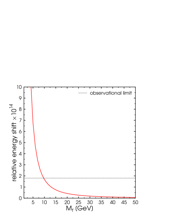
FIG. 3.: The relative energy shift of the S1-S2 hydrogen level from usual uncertainty to generalised uncertainty as a function of the new scale $M_{f}$. The horizontal line represents the accuracy of todays experiment. Values of energy shift above the observation limit and therefore values of $M_{f}<\approx$ 10 GeV are ruled out.

V The Dirac Equation

In ordinary relativistic quantum mechanics the Hamiltonian of the Dirac particle is

$$\hat{H}={\rm i}\hbar\partial_{0}=\gamma_{0}\left({\rm i}\hbar\gamma^{i}\partial_{i}+m\right).$$ (82)

This leads to the Dirac Equation

$$(p/-m)\psi = 0,$$ (83)

with the following standard abbreviation $\gamma^{\nu}A_{\nu}:=A/$ and $p_{\nu}={\rm i}\hbar\partial_{\nu}$. To include the modifications due to the generalised uncertainty principle, we start with the relation

$$\hat{E}=\gamma_{0}\left(\gamma^{i}\hat{p}_{i}(k)+m\right)$$ (84)

as the first step to quantisation. Including the alternated momentum wave vector relation $\hat{p}(k)$, this yields again Eq. (83) with the modified momentum operator

$$(p/(k)-m)\psi = 0\quad.$$ (85)

This equation is Lorentz invariant by construction (see our general discussion in section III A). Since it contains – in position representation – 3rd order derivatives in space coordinates, it contains 3rd order time-derivatives too. In case (a) we can solve the equation for a first order time derivative by using the energy mass shell condition $E^{2}=p^{2}+m^{2}$. This leads effectively to a replacement of time derivatives by space derivatives:

$$\hbar\hat{\omega}\approx\hat{E}-\hat{E}^{3}/M_{f}^{2}=\hat{E}\left(1-\frac{\hat{p}^{i}\hat{p}_{i}+m^{2}}{M_{f}^{2}}\right)\quad.$$ (86)

Therefore we obtain the following expression of the Dirac Equation in case (a):

$${\rm i}\hbar\partial_{0}|\psi\rangle \approx \gamma_{0}\left({\rm i}\hbar\gamma^{i}\partial_{i}+m\right)\left(1+L_{f}^{2}\partial^{i}\partial_{i}-\frac{m^{2}}{M_{f}^{2}}\right)|\psi\rangle.$$ (87)

However, the equation (85) could be considered to be in the more aesthetic form, especially – except in cases we ask for the time evolution – we will surely prefer its obvious Lorentz invariant appearance.

VI The Klein Gordon Equation

Analogously to the derivation of the Dirac Equation in the framework of a generalised uncertainty principle, we can obtain the modification of the Klein Gordon Equation. Again, starting with the energy momentum relation:

$$E^{2}-p^{2}=m^{2},$$ (88)

we obtain

$$\eta^{\mu\nu}\hat{p}_{\nu}\hat{p}_{\mu}\psi=m^{2}\psi.$$ (89)

Including the changed momentum wave vector relation $\hat{p}(k)$, this yields the former Klein Gordon equation up to the modified momentum operators. Note that the square of the generalised Dirac Equation (85) still fulfils the generalised Klein Gordon Equation (89). In case (a), one obtains the following explicit expression in terms of derivative operators:

$$-\hbar^{2}\eta^{\mu\nu}\left(\partial_{\nu}-\frac{L_{f}^{2}}{3}\partial^{3}_{\nu}\right)\left(\partial_{\mu}-\frac{L_{f}^{2}}{3}\partial^{3}_{\mu}\right)\psi=m^{2}\psi.$$ (90)

VII QED

A The Fermion Field

The creation and annihilation operators for anti-particles ${}^{-}{\hat{a}}^{{\dagger}}_{r}(p),{}^{-}\hat{a_{r}}(p)$ and for particles ${}^{+}{\hat{a}}^{{\dagger}}_{r}(p),{}^{+}\hat{a}_{r}(p)$, respectively, obey the following anti commutation relations:

$$\left[{}^{+}\hat{a}^{{\dagger}}_{r}(p),{}^{+}\hat{a}_{s}(p^{\prime})\right]_{+} = \delta_{rs}\delta(\vec{p}-\vec{p}^{\prime})\prod_{\nu}\frac{\partial p_{\nu}}{\partial k_{\nu}}\quad,$$ (91)

$$\left[{}^{-}\hat{a}^{{\dagger}}_{r}(p),{}^{-}\hat{a}_{s}(p^{\prime})\right]_{+} = \delta_{rs}\delta(\vec{p}-\vec{p}^{\prime})\prod_{\nu}\frac{\partial p_{\nu}}{\partial k_{\nu}}\quad.$$ (92)

and the remaining anti commutators are identically zero. The field operator $\psi_{p,r}({\underline{\bf x}})$ can be expanded in terms of these creation and annihilation operators in the following way:

$$\psi_{p,r}({\underline{\bf x}}) = \sum_{r}\int\frac{{\rm d}^{3}p}{(2\pi)^{3/2}}\sqrt{\frac{m}{\hbar\omega}}\;{\rm det}\left(\frac{\partial k_{\nu}}{\partial p_{\mu}}\right)\;\times$$ (93)

$$\bigg{(} {}^{+}\hat{a}_{r}(p)u(p,r){\rm e}^{{\rm i}k^{\nu}x_{\nu}}+{}^{-}\hat{a}^{{\dagger}}_{r}(p)v(p,r){\rm e}^{-{\rm i}k^{\nu}x_{\nu}}\bigg{)}.$$ (94)

In this expression we used the following conventions for the spinors:

$$u(p,r) = \frac{p/+m}{\sqrt{2m(E+m)}}u(0,r)\quad,$$ (95)

$$v(p,r) = \frac{-p/+m}{\sqrt{2m(E+m)}}v(0,r)\quad,$$ (96)

where $v(0,r),u(0,r)$ are the unit spinors in the rest frame, $\vec{p}=0$. These spinors obey the relations

$$\sum_{r}u(p,r)\bar{v}(p,r) = \frac{p/+m}{2m}\quad,$$ (97)

$$\sum_{r}v(p,r)\bar{v}(p,r) = \frac{p/-m}{2m}\quad.$$ (98)

The Lagrangian density which yields the Dirac equation for the free fermion field is

$${\cal L}(\bar{\psi},\psi)={\rm i}\bar{\psi}(p/(k)-m)\psi\quad.$$ (99)

So we can read off [54, 55] the free Feynman propagator for the fermions ${}^{\rm f}\Delta_{\mu\nu}$ in momentum representation is

$${}^{\rm f}\Delta_{\mu\nu}=\frac{1}{p/(k)-m+{\rm i}\epsilon}\quad.$$ (100)

Alternatively, one could have derived this by evaluating time ordered products of the field operators using the relations (91) - (98). Evaluating the Feynman propagator by considering these time ordered products yields again (100) due to the cancellations of the momentum measures by the respective inverse terms.

To obtain the Hamiltonian density ${\cal H}$ in the position representation ${\cal H}(x)$, one has to treat the Lagrangian density as a function of all appearing higher derivative terms ${\cal L}(\psi,\partial_{\nu}\psi,\partial^{2}_{\mu\nu}\psi,\partial^{3}_{\mu\nu\kappa}\psi)$ (see 99). Therefore we have to introduce to canonically conjugated momenta:

$$\pi_{1}(x) = \frac{\partial{\cal L}_{{\rm f}}}{\partial(\partial_{t}\psi(x))}={\rm i}\psi^{{\dagger}}(x)\quad,$$ (101)

$$\pi_{2}(x) = \frac{\partial{\cal L}_{{\rm f}}}{\partial(\partial^{3}_{t}\psi(x))}=-{\rm i}\frac{L_{f}^{2}}{3}\psi^{{\dagger}}(x)\quad.$$ (102)

The Hamiltonian density can now be derived using this generalised scheme:

$${\cal H}(x) = \pi_{1}\partial_{t}\psi(x)+\pi_{2}\partial^{3}_{t}\psi(x)-{\cal L}$$ (103)

$$= {\rm i}\psi^{{\dagger}}(x)\partial_{t}\left(1-\frac{L_{f}^{2}}{3}\partial^{2}_{t}\right)\psi(x)\quad.$$ (104)

B The Photon Field

Starting from the expression of the energy density of the photon field in the framework of a generalised uncertainty principle:

$$E = \frac{1}{4}\tilde{F}^{\mu\nu}\tilde{F}_{\mu\nu}\quad,$$ (105)

with the modified field strength tensor, in case (a) explicitly given by

$$\tilde{F}_{\mu\nu} = \partial_{\mu}\left(1-\frac{L_{f}^{2}}{3}\partial^{2}_{\mu}\right)A_{\nu}-\partial_{\nu}\left(1-\frac{L_{f}^{2}}{3}\partial^{2}_{\nu}\right)A_{\mu}\quad,$$ (106)

we derive the corresponding Lagrangian density:

$${\cal L}=-\frac{1}{4}\tilde{F}^{\mu\nu}\tilde{F}_{\mu\nu}\quad.$$ (107)

This can also be expressed as

$${\cal L} = -\frac{1}{4}A^{\mu}{\cal{D}}_{\mu\nu}A^{\nu}$$ (108)

with

$${\cal{D}}_{\mu\nu} = \left(\stackrel{{\scriptstyle\leftarrow}}{{\partial_{\mu}}}-\frac{L_{f}^{2}}{3}\stackrel{{\scriptstyle\leftarrow}}{{\partial_{\mu}^{3}}}\right)\left(\stackrel{{\scriptstyle\rightarrow}}{{\partial_{\nu}}}-\frac{L_{f}^{2}}{3}\stackrel{{\scriptstyle\rightarrow}}{{\partial_{\nu}^{3}}}\right)\quad.$$ (109)

Using this Lagrangian density the interaction-free Feynman photon propagator ${}^{\rm p}\Delta_{\mu\nu}$ (in Feynman gauge) can unambiguously determined to be

$${}^{\rm p}\Delta_{\mu\nu}=-\frac{1}{p^{2}(k)+{\rm i}\epsilon}\quad.$$ (110)

C Coupling

We introduce the electrodynamical gauge invariant coupling as usual via $\partial_{\nu}\to D_{\nu}:=\partial_{\nu}-{\rm i}eA_{\nu}$ in (99). We keep as the approximation in case (a) only terms up to first order in $e$ and terms up to quadratic order in $1/M_{f}$, admixtures of both are neglected. This actually yields the familiar interaction Lagrangian

$${\cal L}_{i}=-e\bar{\psi}\gamma_{\nu}\psi A^{\nu}\quad.$$ (111)

As before, we can derive ${\cal H}_{{\rm i}}$, and find as usual

$${\cal L}_{i}=-{\cal H}_{{\rm i}}\quad.$$ (112)

D Perturbation Theory

We see now that the only modification in computing a cross-section arises from the different normalisation of the particle states and the different volume factors due to a suppressed occupation of momentum space at high energies. Let us consider now as an important example the Compton scattering and ask for the QED prediction at tree level in perturbation theory. We are using the following notation:

$${\underline{\bf p}}_{{\rm i}1}=(\vec{p}_{{\rm i}1},E_{{\rm i}1}) : \mbox{initial electron}\quad,$$ (113)

$${\underline{\bf p}}_{{\rm i}2}=(\vec{p}_{{\rm i}2},E_{{\rm i}2}) : \mbox{initial photon}\quad,$$ (114)

$${\underline{\bf p}}_{{\rm f}1}=(\vec{p}_{{\rm f}1},E_{{\rm f}1}) : \mbox{final electron}\quad,$$ (115)

$${\underline{\bf p}}_{{\rm f}2}=(\vec{p}_{{\rm f}2},E_{{\rm f}2}) : \mbox{final photon}\quad,$$ (116)

and

$${\underline{\bf p}}_{{\rm i}} = {\underline{\bf p}}_{{\rm i}1}+{\underline{\bf p}}_{{\rm i}2}\quad,$$ (117)

$${\underline{\bf p}}_{{\rm f}} = {\underline{\bf p}}_{{\rm f}1}+{\underline{\bf p}}_{{\rm f}2}\quad,$$ (118)

$$E = E_{{\rm i}1}+E_{{\rm i}2}=E_{{\rm f}1}+E_{{\rm f}2}\quad.$$ (119)

The expression of the $S$-Matrix element in the realm of the generalised uncertainty principle is:

$$\tilde{S}_{{\rm fi}}=(2\pi)^{4}\tilde{M}_{{\rm fi}}\delta({\underline{\bf p}}_{{\rm i}}-{\underline{\bf p}}_{{\rm f}})\prod_{\nu}\frac{\partial p_{\nu}}{\partial k_{\nu}}\Bigg{|}_{{\underline{\bf p}}_{{\rm i}}={\underline{\bf p}}_{{\rm f}}}$$ (120)

The probability of the initial particles to wind up in a certain range of momentum space d$P($i$\to$ f$)$ can be obtained in the usual way by putting the system into a finite box with volume $V$. Since the measure of momentum space is modified this yields a Jacobian determinant for every final particle. For our example this reads

$${\rm d}P({\rm i}\to{\rm f})=\left(\frac{(2\pi)^{3}}{V}\right)^{2}|\tilde{S}_{{\rm fi}}|^{2}\hbar^{2}{\rm d}^{3}p_{\rm f1}{\rm d}^{3}p_{\rm f2}\left(\prod_{\nu}\frac{\partial k_{\nu}}{\partial p_{\nu}}\right)^{2}$$ (121)

and the differential cross-section for two particles in the final state is then

$${\mathrm{d}}\tilde{\sigma}\left({\rm i}\to{\rm f}\right)=\hbar^{2}(2\pi)^{4}\frac{1}{\Phi V}|\tilde{M}_{{\rm fi}}|^{2}\frac{E_{{\rm f}1}E_{{\rm f}2}|p_{{\rm f}2}|}{E}\prod_{\nu}\frac{\partial k_{\nu}}{\partial p_{\nu}}{\mathrm{d}}\Omega\quad.$$ (122)

Here $\Phi$ is the flux. In the laboratory system, we have $\vec{p}_{{\rm i}1}=0,E_{{\rm i}1}=m,E_{{\rm f}1}=m+E_{{\rm i}2}-E_{{\rm f}2}$, therefore $\Phi V=1$. This leads to the following expression in the laboratory system:

$${\mathrm{d}}\tilde{\sigma}\left({\rm i}\to{\rm f}\right)=\hbar^{2}(2\pi)^{4}|\tilde{M}_{{\rm fi}}|^{2}\frac{E_{{\rm f}1}E_{{\rm f}2}^{3}}{mE_{{\rm i}2}}\prod_{\nu}\frac{\partial k_{\nu}}{\partial p_{\nu}}{\mathrm{d}}\Omega\quad.$$ (123)

Explicitly, in case (a) and in the laboratory system, we have

$$\prod_{\nu}\frac{\partial p_{\nu}}{\partial k_{\nu}}=\hbar^{4}\left(1+\frac{E_{{\rm i}2}^{2}}{M_{f}^{2}}\right)\left(1+\frac{(m+E_{{\rm i}2})^{2}}{M_{f}^{2}}\right)$$ (124)

and the Jacobi determinant of the inverse function in Eq. (123) is just given by the inverse of this expression.

The amplitude summed over all possible initial and final polarisations, $e_{{\rm i}}$, $e_{{\rm f}}$, remains in the well known standard form [56]

$$\frac{1}{4}\sum_{{\sigma}_{{\rm i}}\sigma_{{\rm f}}e_{{\rm i}}e_{{\rm f}}}|\tilde{M}_{{\rm fi}}| = \frac{e^{4}}{64(2\pi)^{6}}\frac{1}{\omega_{{\rm f}2}\omega_{{\rm i}2}\omega_{{\rm f}1}\omega_{{\rm i}1}}\;\times$$ (126)

$$\left[\frac{E_{{\rm i}2}}{E_{{\rm f}2}}+\frac{E_{{\rm f}2}}{E_{{\rm i}2}}-1+\cos^{2}\theta\right]$$

with $\omega_{\rm index}=\omega(E_{\rm index})$. All this put together yields

$$\frac{1}{4}\sum_{\sigma_{{\rm i}}\sigma_{{\rm f}}e_{{\rm i}}e_{{\rm f}}}\frac{{\mathrm{d}}\tilde{\sigma}}{{\mathrm{d}}\Omega}\left({\rm i}\to{\rm f}\right) = \frac{\hbar^{2}e^{4}}{32\pi^{2}}\prod_{\nu}\frac{\partial k_{\nu}}{\partial p_{\nu}}\;\times$$ (127)

$$\frac{(m+E_{{\rm i}2}-E_{{\rm f}2})E_{{\rm f}2}^{3}}{\omega_{{\rm f}2}\omega_{{\rm i}2}\omega_{{\rm f}1}\omega_{{\rm i}1}mE_{{\rm i}2}} \left[\frac{E_{{\rm i}2}}{E_{{\rm f}2}}+\frac{E_{{\rm f}2}}{E_{{\rm i}2}}-1+\cos^{2}\theta\right]\quad.$$ (128)

This example illustrates how modified cross sections $\tilde{\sigma}$ in scattering processes with two initial and two final states can be obtained from the unmodified cross sections $\sigma$. This relation is given by the following formula:

$$\frac{{\mathrm{d}}\tilde{\sigma}}{{\mathrm{d}}\sigma}=\prod_{n}\frac{E_{n}}{\omega_{n}}\prod_{\nu}\frac{\partial k_{\nu}}{\partial p_{\nu}}\Bigg{|}_{{\underline{\bf p}}_{{\rm i}}={\underline{\bf p}}_{{\rm f}}}\quad.$$ (129)

From the steps of calculation it can be seen that this result holds in higher order perturbation theory, too. The modification enters through the energies of the in- and outgoing particles and their momenta spaces, only. However, when incorporating higher orders one has to bear in mind, that we approximated the interaction Hamiltonian by neglecting terms of order $\alpha/M_{f}^{2}$. These terms should reappear at higher energies leading to the necessity of a reordering of the corresponding perturbation series. To be precise, the full modified SM result contains more terms than one would have taken into account by just using Eq. (129).

Let us interpret this result physically before going any further. There are two factors occurring. The first shows that the physics at a certain energy $\tilde{E}$ of two particles is now rescaled. It is identical to the physics that happened before at a smaller energy $E$ with $E=\hbar\omega(\tilde{E})$. A higher energy is needed within our model to reach the same distance between the particles as in the standard model: To get the same resolution as with the standard uncertainty principle, one has to go to higher energies! Because the cross sections decrease with energy this means our modified cross section predictions are higher at the same energy than those of the standard model. The functional behaviour of the standard model result should be cut at $M_{f}$ and the range up to $M_{f}$ be stretched out to infinity. In particular, only from this factor the cross-section would asymptotically get constant at a value equal to the unmodified standard model result at $M_{f}$.

But there is another factor from the Jacobian, which takes into account that the phase space for the final states is reduced significantly from Planckian energies on. Since ${\bf{\underline{k}}}({\bf{\underline{p}}})$ approaches a constant value, its Jacobian and therefore the relation (129) drops to zero. Putting both effects together, the cross section of our model drops below the unmodified standard model result: As can be seen from the Jacobian in case (b), the cross section drops exponentially with the reaction energy.

The prediction of a dropping cross section in comparison to the unmodified standard model results is quite remarkable. In most models with the assumption of extra dimensions only, an increase of the cross section is predicted. This is due to the enhanced possible reactions when taking into account virtual gravitons (see next section).

It is obvious by construction that in our model no physics can be tested below the distance $L_{f}$. If the new scale is as low as $\approx$ TeV, as suggested by the proposal of Large Extra Dimensions, then an even further increase of the energy that can be delivered by even larger colliders than the next generation can deliver ($\approx$ 14 TeV at LHC) would not yield more insight than the statement that there is such a smallest scale in nature. As was formulated by Giddings this would be “the end of short distance physics” [57, 58]. However, this was mentioned in a different context. In our approach the production of tiny black holes is not yet possible at center of mass (c.o.m.) energies $\sqrt{s}\approx M_{f}$, because the distance needed for two partons of energy $\approx M_{f}$ to collapse and form a black hole is just $L_{f}$, but the particles can not get that close any longer. (This might happen then at higher energies, see [1].) Therefore, we are most interested in testing the present model in ultra high energetic cosmic ray experiments, like the extended air-shower measurements at KASCADE-Grande and at the Pierre Auger Observatory [59], which allows a hundredfold c.o.m.-energy increase over the LHC energies.

For energy $\sqrt{s}$ ($m_{\tau},m_{\mu}\ll\sqrt{s}$) , Eq. (129) yields the simple expression with the functions inserted in the c.o.m. system

$$\frac{{\mathrm{d}}\tilde{\sigma}}{{\mathrm{d}}\sigma} = \frac{s^{2}}{(2M_{f})^{4}}\left(\tanh\left(\frac{\sqrt{s}}{2M_{f}}\right)\right)^{-4}\times$$ (131)

$$\left(\cosh^{2}\left(\frac{\sqrt{s}}{M_{f}}\right)\right)^{-2}.$$

We have used this functional behaviour to get the connection to the measured data of the LEP2 collaboration, [60], $e^{+}e^{-}\to\mu^{+}\mu^{-}$ and $e^{+}e^{-}\to\tau^{+}\tau^{-}$ cross-sections. The derived factor is independent of the scattering angle. Hence, it holds for the total cross-section, as shown in Fig 4. In this context, note that possible limits on physics beyond the standard model in LEP2 fermion pair production data have already been discussed in [61] from the experimental view – this is one of the new trends in high-energy physics.

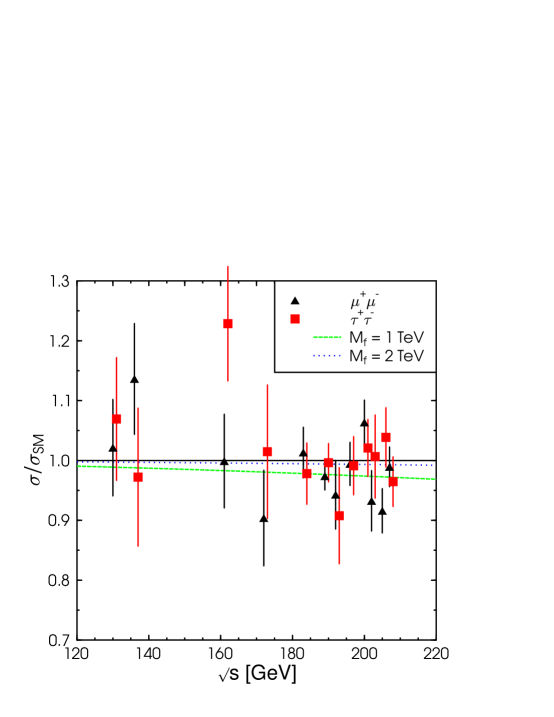
FIG. 4.: The ratio of $e^{+}e^{-}\to\mu^{+}\mu^{-},\tau^{+}\tau^{-}$ cross sections calculated with the generalised and the ordinary uncertainty principle. Data is taken from [60].

VIII Gravitons

Many prominently discussed collider signatures of LXDs are connected to the virtual and real graviton $G$ production processes. Extensive studies of this subject already exist in the literature (see e.g. [62, 63, 64]). In these scenarios Kaluza-Klein excitations are given in steps $n_{a}/R$. The maximum possible frequency $n_{a}=RM_{f}$ is in these scenarios the natural cutoff. (For simplicity we have set the compactification radii of all extra dimensions to be equal.)

We start with the real gravitons, which are important at energies $>M_{f}$ due to the significant increase of the corresponding phase space factor. In order to estimate the $e^{+}e^{-}\to\gamma G$ cross section in the context of the modified uncertainty principle, we start with the relation:

$$\sigma(e^{+}e^{-}\to\gamma G)\propto\frac{e^{2}}{m_{p}^{2}}N(\sqrt{s})\quad,$$ (132)

we have to calculate the number of possible final states with $E=\sqrt{s}/2$ in the c.o.m. system, which is called $N(\sqrt{s}/2)$. $N(\sqrt{s}/2)$ can be obtained using (with $\Delta m\rightarrow{\rm d}m$):

$$\frac{{\rm d}m}{{\rm d}n_{a}}=\frac{1}{R}\frac{\partial E}{\partial\omega}\quad,$$ (133)

where $m$ is the apparent mass of the excitation of the respective Kaluza-.Klein state:

$$m^{2}=p_{\perp}^{2}=\sum_{a=4}^{d+4}\left(E(\omega_{a})\right)^{2}\;,\hskip 8.5359pt{\rm with}\quad\omega_{a}=\frac{n_{a}}{R}\quad.$$ (134)

Using Eq. (1) and the above expressions one obtains for the number of final states:

$$N(\sqrt{s}) = \Omega_{(d-1)}R^{d}\int_{0}^{\sqrt{s}/2}{\rm d}m\;\omega(m)^{d-1}\frac{\partial\omega}{\partial E}$$ (135)

$$= V_{(d)}\frac{m_{p}^{2}}{M_{f}^{d+2}}\omega(\sqrt{s}/2)^{d}$$ (136)

with $\Omega_{(d-1)}$ being the surface of the $d$-dimensional unit-sphere and $V_{(d)}$ being its volume:

$$\Omega_{(d-1)} = \frac{2\pi^{d/2}}{\Gamma\left(d/2\right)}=dV_{(d)}\quad.$$ (137)

These considerations yield the following estimation of the real graviton production cross section:

$$\sigma(e^{+}e^{-}\to\gamma G)\propto\frac{e^{2}}{\omega(\sqrt{s}/2)^{2}}\left(\frac{\omega(\sqrt{s}/2)}{M_{f}}\right)^{d+2}.$$ (138)

The exact result for the fermion to real graviton plus $\gamma$ cross section in the framework of the generalised uncertainty principle depends on the amplitude of the process and on the spin-sums. However, for the following general considerations the estimate (138) is sufficient. This cross-section would be of the same importance with SM processes if $\omega$ equals $M_{f}$, which is here only possible asymptotically. Therefore, real gravitons are produced at a lower rate when a generalised uncertainty principle is employed than expected from LXD scenarios without the generalised uncertainty relation. As a consequence, constraints (e.g. by energy loss) from real graviton emission should be reanalysed carefully in the context of the minimal length proposal.

Now, let us turn to the virtual graviton production. The free graviton propagator from [62] for $G_{m}$ (Graviton of apparent mass $m$) is generalised to:

$${}^{\rm G}\Delta=\frac{P_{\mu\nu\alpha\beta}}{p(k)^{2}-m^{2}}\quad,$$ (139)

where $P_{\mu\nu\alpha\beta}$ is the graviton polarisation tensor (the exact form of the polarisation tensor can be found in [62]). To calculate the complete graviton exchange amplitudes, the amplitudes for different $m$ have to be summed up. The ultraviolet-divergence of this sum has to be fixed by introducing a cut-off parameter $\Lambda$ that is of order $M_{f}$. Such an ad hoc introduction of a cut-off parameter is from a theoretical point of view always somewhat dissatisfying. In the context of the generalised uncertainty relation such a cut-off parameter is naturally included from first principals via the minimal length scale $L_{f}$. Therefore, no ad hoc cut-off parameter is needed:

$$\sum_{n}\frac{1}{p^{2}-m^{2}}=\Omega_{(d-1)}\int_{0}^{\infty}{\rm d}m\frac{m^{d+1}}{p^{2}-m^{2}}\frac{\partial\omega}{\partial E}.$$ (140)

Using case (b), it is easy to see that the UV-end converges for all $d$ due to the exponential suppression of the momentum measure. To calculate this integral, it can be expanded in a power series in $\sqrt{s}/M_{f}$, as given in [62] using the cut-off parameter. In our approach the expansion coefficients could be calculated right away. We will not perform this analysis here. This result will not yield a more profound relation between the exact parameters and the expansion coefficients, since in our approach the arbitrariness lies in the exact form of the function $E(\omega)$ applied, or its expansion coefficients, respectively.

Even if the details of graviton production are not further examined in this paper, one can now conclude that within our model the cross-sections (e.g. the above calculated $\tilde{\sigma}(e^{+}e^{-}\to f^{+}f^{-})$) are modified in a different way than in the scenario with LXDs only. The virtual graviton exchange increases the cross-section, but the squeezing of the momentum space decreases it. So we have two effects of a similar magnitude which are working against each other. Therefore, measurable deviations may occur only at energies higher than $M_{f}$. If one is looking for signatures beyond the standard model, one should focus instead on observables that are not too sensitive to the generalised uncertainty, such as modifications in the spin distribution due to the exchange of a spin 2- particle or the appearance of processes that are forbidden by the standard-model. Furthermore, we want to mention that most of the constraints on the $M_{f}$ scale are weakened in our scenario.

IX Conclusions

We introduce modifications of quantum mechanics caused by the existence of a minimal length scale $L_{f}$. We show that our approach is consistent with other calculations on this topic. Assuming the recent proposition of Large Extra Dimensions, the new scale might be accessible in colliders. We use perturbation theory to derive the $e^{+}e^{-}\to f^{+}f^{-}$ cross sections with an approximated interaction Hamiltonian. We compare our results to recent data and find that the limits on the new scale are compatible to those from different experimental constraints: $1/L_{f}\approx>1$ TeV. Our model combines both Large Extra Dimensions and the minimal length scale and predicts dropping cross sections relative to the standard model cross sections. Further, we argue that the analysed Planckian effects hinder the emergence of other effects which are predicted above $\approx 1$ TeV, such as black hole and graviton production.

REFERENCES

- [1] D. J. Gross and P. F. Mende, Nucl. Phys. B 303 (1988) 407.
- [2] D. Amati, M. Ciafaloni and G. Veneziano, Phys. Lett. B 216 (1989) 41.
- [3] E. Witten, Phys. Today, 49 (1996) 24.
- [4] L. J. Garay, Int. J. Mod. Phys. A 10 (1995) 145 [arXiv:gr-qc/9403008] .
- [5] A. Kempf, [arXiv:hep-th/9810215] .
- [6] A. Kempf, G. Mangano and R. B. Mann, Phys. Rev. D 52 (1995) 1108 [arXiv:hep-th/9412167].
- [7] A. Kempf and G. Mangano, Phys. Rev. D 55 (1997) 7909 [arXiv:hep-th/9612084].
- [8] S. F. Hassan and M. S. Sloth, [arXiv:hep-th/0204110].
- [9] U. H. Danielsson, Phys. Rev. D 66 (2002) 023511 [arXiv:hep-th/0203198].
- [10] S. Shankaranarayanan, Class. Quant. Grav. 20 (2003) 75 [arXiv:gr-qc/0203060].
- [11] L. Mersini, M. Bastero-Gil and P. Kanti, Phys. Rev. D 64 (2001) 043508 [arXiv:hep-ph/0101210].
- [12] A. Kempf, Phys. Rev. D 63 (2001) 083514 [arXiv:astro-ph/0009209].
- [13] A. Kempf and J. C. Niemeyer, Phys. Rev. D 64 (2001) 103501 [arXiv:astro-ph/0103225].
- [14] J. Martin and R. H. Brandenberger, Phys. Rev. D 63 (2001) 123501 [arXiv:hep-th/0005209].
- [15] R. Easther, B. R. Greene, W. H. Kinney and G. Shiu, [arXiv:hep-th/0110226].
- [16] R. H. Brandenberger and J. Martin, Mod. Phys. Lett. A 16 (2001) 999 [arXiv:astro-ph/0005432].
- [17] N. Arkani-Hamed, S. Dimopoulos and G. Dvali, Phys. Lett. B 429, 263-272 (1998) [arXiv:hep-ph/9803315].
- [18] I. Antoniadis, N. Arkani-Hamed, S. Dimopoulos and G. Dvali, Phys. Lett. B 436, 257-263 (1998) [arXiv:hep-ph/9804398].
- [19] N. Arkani-Hamed, S. Dimopoulos and G. Dvali, Phys. Rev. D 59, 086004 (1999) [arXiv:hep-ph/9807344] .
- [20] L. Randall and R. Sundrum, Phys. Rev. Lett. 83 (1999) 4690 [arXiv:hep-th/9906064].
- [21] L. Randall and R. Sundrum, Phys. Rev. Lett. 83 (1999) 3370 [arXiv:hep-ph/9905221].
- [22] K. R. Dienes, E. Dudas and T. Gherghetta, published in Boston 1998, Particles, strings and cosmology, p. 613-620, arXiv:hep-ph/9807522.
- [23] Y. Uehara, [arXiv:hep-ph/0203244] .
- [24] K. Cheung, [arXiv:hep-ph/0003306] .
- [25] S. Cullen, M. Perelstein and M. E. Peskin, Phys. Rev. D 62 (2000) 055012 [arXiv:hep-ph/0001166].
- [26] S. Cullen and M. Perelstein, Phys. Rev. Lett. 83, 268 (1999) [arXiv:hep-ph/9903422] .
- [27] J. Hewett and M. Spiropulu, [arXiv:hep-ph/0205106].
- [28] V. Barger, T. Han, C. Kao and R.-J. Zhang, Phys. Lett. B 461, 34 (1999), [arXiv:hep-ph/9905474] .
- [29] C. Hanhart, J. A. Pons, D. R. Phillips and S. Reddy, Phys. Lett. B 509 1-9 (2001), [arXiv:astro-ph/0102063].
- [30] E. A. Mirabelli, M. Perelstein and M. E. Peskin, Phys. Rev. Lett. 82 2236-2239 (1999) [arXiv:hep-ph/9811337].
- [31] G. F. Giudice, R. Rattazzi and J. D. Wells, Nucl.Phys. B544 3-38 (1999) [arXiv:hep-ph/9811291] .
- [32] G. F. Giudice, R. Rattazzi and J. D. Wells, Nucl.Phys. B595 250-276 (2001) [arXiv:hep-ph/0002178].
- [33] J. L. Hewett, Phys.Rev.Lett. 82 4765-4768 (1999) [arXiv:hep-ph/9811356].
- [34] S. Nussinov and R. Shrock, Phys.Rev. D59 105002 (1999) [arXiv:hep-ph/9811323].
- [35] T. G. Rizzo, [arXiv:hep-ph/9910255] .
- [36] P.C. Argyres, S. Dimopoulos, and J. March-Russell, Phys. Lett. B441, 96 (1998) [arXiv:hep-th/9808138].
- [37] S. B. Giddings, [arXiv:hep-ph/0110127].
- [38] I. Mocioiu, Y. Nara and I. Sarcevic, Phys. Lett. B 557 (2003) 87 [arXiv:hep-ph/0301073].
- [39] A. V. Kotwal and C. Hays, Phys. Rev. D 66 (2002) 116005 [arXiv:hep-ph/0206055].
- [40] Y. Uehara, Prog. Theor. Phys. 107, 621 (2002) [arXiv:hep-ph/0110382].
- [41] R. Emparan, M. Masip and R. Rattazzi, Phys. Rev. D 65, 064023 (2002) [arXiv:hep-ph/0109287].
- [42] S. Hossenfelder, S. Hofmann, M. Bleicher and H. Stocker, Phys. Rev. D 66 (2002) 101502 [arXiv:hep-ph/0109085].
- [43] A. Ringwald and H. Tu, Phys. Lett. B 525 (2002) 135 [arXiv:hep-ph/0111042].
- [44] D. Kazanas and A. Nicolaidis, Gen. Rel. Grav. 35 (2003) 1117 [arXiv:hep-ph/0109247].
- [45] G. Amelino-Camelia, Nature 418 (2002) 34 [arXiv:gr-qc/0207049].
- [46] J. Magueijo and L. Smolin, Phys. Rev. Lett. 88 (2002) 190403 [arXiv:hep-th/0112090].
- [47] M. Toller, arXiv:hep-th/0301153.
- [48] C. Rovelli and S. Speziale, Phys. Rev. D 67 (2003) 064019 [arXiv:gr-qc/0205108].
- [49] I. Dadic, L. Jonke and S. Meljanac, Phys. Rev. D 67 (2003) 087701 [arXiv:hep-th/0210264].
- [50] A. Kempf, J. Phys. A 30 (1997) 2093 [arXiv:hep-th/9604045].
- [51] F. Brau, J. Phys. A 32 (1999) 7691 [arXiv:quant-ph/9905033].
- [52] R. Akhoury and Y. P. Yao, arXiv:hep-ph/0302108.
- [53] T. Udem, Phys. Rev. Lett., 79, 2646 (1997)
- [54] L. H. Ryder, “Quantum Field Theory”, 2nd edition, Cambridge University Press (2001).
- [55] W. Greiner, J. Reinhardt, “Field Quantization”, Springer Verlag, (May 1996).
- [56] S. Weinberg “The Quantum Theory of Fields”, Vol. I, Cambridge
- [57] T. Banks and W. Fischler, arXiv:hep-th/9906038.
- [58] S. B. Giddings and S. Thomas, Phys. Rev. D 65 (2002) 056010 [arXiv:hep-ph/0106219].
-
[59]
KASCADE-Grande: http://www-ik.fzk.de/KASCADE_home.html;
AUGER: http://www.auger.org - [60] LEPEWWG subgroup, D. Bourikov et al., LEP2ff/01-02 (2001).
- [61] G. Abbiendi, arXiv:hep-ex/0111014.
- [62] G. F. Giudice, R. Rattazzi and J. D. Wells, Nucl. Phys. B 544, 3 (1999) [arXiv:hep-ph/9811291].
- [63] J. Hewett and M. Spiropulu, Ann. Rev. Nucl. Part. Sci. 52 (2002) 397 [arXiv:hep-ph/0205106].
- [64] T. Han, J. D. Lykken and R. J. Zhang, Phys. Rev. D 59 (1999) 105006 [arXiv:hep-ph/9811350].