The Effects of Quantum Deformations
on the Spectrum of Cosmological Perturbations

Abstract

We consider a quantum deformation of the wave equation on a cosmological background as a toy-model for possible trans-Planckian effects. We compute the power spectrum of scalar and tensor fluctuations for power-law inflation, and find a noticeable deviation from the standard result. We consider de Sitter inflation as a special case, and find that the resulting power spectrum is scale invariant. For both inflationary scenarios the departure from the standard spectrum is sensitive to the size of the deformation parameter. A modulation in the power spectrum appears to be a generic feature of the model.

I Introduction

Recently a lot of attention has been devoted to the possibility that Planck scale physics might leave an imprint on the cosmic microwave background (CMB). The temperature anisotropies of the CMB in fact arise from quantum fluctuations generated in the early universe and stretched by inflation to observable scales. Thus, length scales which are now of cosmological size could have been below the Planck length at the beginning of inflation, and could therefore carry the imprint of trans-Planckian physics. Within the standard theory of cosmological perturbations, fluctuations are assumed to originate in the infinite past with an infinitely small size. However, near the Planck scale the structure of space-time is believed to be modified by quantum gravitational effects, with the Planck length playing the role of a physical cutoff. Such modifications could affect the evolution of cosmological perturbations, possibly even changing the predictions of standard inflation.

Several groups have considered models for physics above the Planck scale, and computed the resulting corrections to the standard spectrum of fluctuations. These approaches have included nonlinear dispersion relations Martin:2000xs ; Brandenberger:2000wr ; Amelino-Camelia:1999zc ; Niemeyer ; Mersini:2001su ; Starobinsky:2001kn ; BM1 ; Brandenberger:2002hs ; NP2 ; LLMU ; BJM , short-distance modifications to quantum-mechanical commutation relations Kempf ; CGS ; EGKS ; KempfN ; HS , models based on noncommutative geometry Lizzi:2002ib ; Brandenberger:2002nq ; Huang:2003zp , non-standard initial conditions Danielsson:2002kx ; Danielsson:2002qh ; Danielsson:2002mb ; Goldstein:2002fc ; Alberghi:2003am ; Armendariz-Picon:2003gd and effective field theory techniques Shenker . Also, more recent work has been based on ‘minimal’ models, where the specific nature of trans-Planckian physics is not assumed, but rather described by the boundary conditions imposed on the modes at the cutoff scale Danielsson:2002kx ; Easther:2002xe ; Niemeyer:2002kh ; Martin:2003kp . For a detailed review, see Martin:2003kp .

What emerges from these proposals is the possibility of obtaining substantial corrections to the standard CMB power spectrum, showing that inflation can indeed carry the signature of physics close to the string (Planck) scale. However, it is also apparent that the conclusions reached are extremely sensitive to the specific short-distance modifications employed and to the choices of initial conditions. Due to the lack of a fundamental theory of quantum gravity, many of the models that have been brought forth are based on ad hoc modifications to short-distance physics. Thus, it is not surprising that they yield different predictions. Still, until we have a more fundamental theory of gravity, a bottom-up approach to modeling very high energy physics is valuable per se, and so is the effort to construct viable cosmological scenarios that might be tested by looking at the CMB temperature anisotropies.

Although slightly different, most of the models considered above share the idea that the structure of space-time is endowed with a fundamental length, usually taken to be the Planck length $l_{P}=M_{P}^{-1}$, corresponding to a high-energy cutoff. It is the presence of such a fundamental scale that is responsible for curing the ultraviolet behavior of the underlying theory, causing processes with energy higher than the cutoff to be suppressed. Also, many quantum gravity models share the notion of a ‘fuzzy’ structure of space-time. For instance, noncommutative geometry provides a natural framework for the formulation of field theories that incorporate fundamental space-time uncertainties. Quantum ($Q$-)deformations, also an example of noncommutativity, provide an additional type of regularization scheme. They are well motivated not only because they are a powerful candidate for regulating divergences, but also because they preserve some of the symmetries of the underlying theory, in the form of quantum symmetries Majid:1990gq . For an example of quantum groups in the context of Planck scale physics and of an algebraic approach to quantum gravity see Majid:1996nt and references therein.

In this work we consider a nonlocal generalization of the wave equation describing cosmological perturbations, in the form of a quantum deformation. The deformation consists in replacing the standard wave operator by its $Q$-deformed counterpart. The new operator is nonlocal by an amount dictated by how much the deformation parameter deviates from its classical value. For similar work in the context of a two-dimensional black hole see Teschner:1999my .

This paper is structured as follows. We start in section I with a brief review of the standard theory of cosmological perturbations. In the next section we find the solution to the $Q$-deformed mode equation at scales higher than the cutoff $\Lambda$, and match it to the standard solution valid below the cutoff scale. We make a conservative choice for the initial conditions, taking a Bunch-Davies-like vacuum. Section III gives the correction to the standard power spectrum for both tensor and scalar fluctuations for the case of power-law inflation. Finally, in section IV we repeat the calculations for the case of de Sitter inflation. We conclude by discussing the implications of our results.

II Standard Inflation

In this section we review very briefly the main features of the theory of cosmological perturbations within the framework of standard inflation. Power-law inflation in a spatially flat FRW universe is described by the metric

$$ds^{2}=dt^{2}-a^{2}(t)d\vec{x}^{2}=a^{2}(\eta)\bigl{(}d\eta^{2}-d\vec{x}^{2}\bigr{)},$$ (1)

where the scale factor is $a(t)=a_{0}t^{n}$ or, in terms of conformal time, $a(\eta)=\alpha_{0}\eta^{\frac{n}{1-n}}$, with $-\infty<\eta<0$ and $\alpha_{0}\equiv\bigl{(}a_{0}(1-n)\bigr{)}^{\frac{n}{1-n}}$. Here $\alpha_{0}$ has dimensions of length. The $n\rightarrow\infty$ limit of power-law inflation yields the de Sitter background, where $a(t)=e^{Ht}$ or $a(\eta)=-\frac{1}{H\eta}$, and $H\equiv\frac{\dot{a}}{a}$ is a constant.

The two types of metric perturbations which are of interest in the early universe are scalar and tensor fluctuations (see Mukhanov:1990me for a review). We start by considering the case of power-law inflation. In Fourier space, the tensor perturbations $u_{k}$ obey the mode equation

$$u^{\prime\prime}_{k}+\bigl{(}k^{2}-\frac{a^{\prime\prime}}{a}\bigr{)}u_{k}=0,$$ (2)

where $k$ is the mode’s comoving momentum and primes indicate derivatives with respect to conformal time. Notice that this is the equation describing a parametric oscillator with a time-dependent frequency.

Scalar perturbations couple to matter, and are responsible for the large scale structure of the universe. The mode equation governing the evolution of scalar fluctuations $v_{k}$ has a similar structure,

$$v^{\prime\prime}_{k}+\bigl{(}k^{2}-\frac{z^{\prime\prime}}{z}\bigr{)}v_{k}=0,$$ (3)

with $a$ replaced by $z=a\frac{\phi_{0}^{\prime}}{{\cal{H}}}$. Here ${\cal{H}}\equiv\frac{a^{\prime}}{a}$ and $\phi_{0}$ denotes the background value of the scalar matter field. In the case of power-law inflation $\phi_{0}^{\prime}$ and ${\cal{H}}$ are both proportional to the same power of $\eta$, so that $\frac{z^{\prime\prime}}{z}=\frac{a^{\prime\prime}}{a}$. Thus, scalar and tensor fluctuations evolve in the same way, and the difference between them becomes manifest only in the final normalization of the power spectrum. For gravitational modes, the power spectrum is given by

$$P_{g}(k)=\frac{k^{3}}{2\pi^{2}}\frac{|u_{k}|^{2}}{a^{2}}$$ (4)

while for scalar perturbations it is given by

$$P_{s}(k)=\frac{k^{3}}{2\pi^{2}}\frac{|v_{k}|^{2}}{z^{2}}.$$ (5)

Using the Friedman equations it can be shown that $z=a\frac{\phi_{0}^{\prime}}{{\cal{H}}}\sim\frac{a}{\sqrt{n}}$ for power-law inflation. This gives

$$P_{s}(k)=\Bigl{(}\frac{{\cal{H}}}{\phi_{0}^{\prime}}\Bigr{)}^{2}P_{g}(k)\sim nP_{g}(k).$$ (6)

The case of de Sitter inflation is more subtle; while the derivation of (4) still holds, that of (5) breaks down, and the spectrum of scalar fluctuations is singular. Thus, we will only consider the spectrum of tensor fluctuations for the de Sitter background. For a recent discussion of this point, see Martin:2003kp .

III Q-deformations and cosmological perturbations

In this work we model the effects of quantum gravity on scales larger than some cutoff energy $\Lambda$ by performing a simple $Q$-deformation of the standard mode equation governing scalar and tensor perturbations. We replace the usual derivatives appearing in the mode equation by a finite difference operator,

$$\partial_{r}f(r)\longrightarrow D_{r}f(r),\ \ D_{r}f(r)\equiv\frac{f(Qr)-f(r)}{Qr-r},$$ (7)

where $Q\>\epsilon\>\mathbb{R}$ and $Q\neq 0,1$ is the parameter that controls the deformation. The finite difference operator reduces to the standard derivative when the deformation parameter is set equal to unity. Some of the properties of $D_{r}$ which will be used throughout this paper are

$$\displaystyle D_{r}\Bigl{(}f_{1}(r)f_{2}(r)\Bigr{)} = \Bigl{(}D_{r}f_{1}(r)\Bigr{)}f_{2}(Qr)+f_{1}(r)D_{r}f_{2}(r),$$ (8)

$$D_{r}r^{n} = [n]r^{n-1},\ \ \text{where}\ \ [n]\equiv\frac{Q^{n}-1}{Q-1},$$ (9)

$$D_{r}e_{Q}^{ar} = ae_{Q}^{ar}\ \ \text{with}\ \ e_{Q}^{ar}=\sum_{n=0}^{\infty}\frac{a^{n}}{[n]!}r^{n},\ \ [n]!\equiv[n][n-1]\dots[1].$$ (10)

Although one can in principle deform all coordinates, we choose a deformation which affects only conformal time, motivated by an analogy with the study of quantum deformations in Anti de Sitter (AdS) space. In fact, it has been suggested Jevicki:1998rr that $Q$-deformations should act only on the radial coordinate of AdS space, which corresponds to the time coordinate in de Sitter space. Thus, the deformed equation of motion valid above the cutoff energy scale $\Lambda$ is given by

$$D^{2}_{\tilde{\eta}}u^{I}_{k}+\Bigl{(}1-\frac{1}{a}D^{2}_{\tilde{\eta}}a\Bigr{)}u^{I}_{k}=0,\ \ \ \ \tilde{\eta}\equiv k\eta.$$ (11)

Notice that while we are explicitly considering tensor fluctuations, the same analysis holds for scalar perturbations. The difference between the two cases will become apparent in the final normalization of the power spectrum. Using $\frac{1}{a}D^{2}_{\tilde{\eta}}a=\bigl{[}\frac{n}{1-n}\bigr{]}\bigl{[}\frac{n}{1-n}-1\bigr{]}\frac{1}{\tilde{\eta}^{2}}$, eq. (11) simplifies to

$$D^{2}_{\tilde{\eta}}u^{I}_{k}+\Bigl{(}1-\frac{C}{\tilde{\eta}^{2}}\Bigr{)}u^{I}_{k}=0,\ \ \ \ C\equiv\Bigl{[}\frac{n}{1-n}\Bigr{]}\Bigl{[}\frac{n}{1-n}-1\Bigr{]}.$$ (12)

If we neglect the $\frac{C}{\tilde{\eta}^{2}}$ term, $f_{k}(-k\eta)\sim e_{Q}^{-ik\eta}$ is a solution of the resulting $Q$-deformed equation of motion. Since in the trans-Planckian region $|k\eta|\gg 1$, we can construct the solution to the full deformed mode equation by making the expansion

$$f_{k}(-k\eta)=e_{Q}^{-ik\eta}\sum_{j=0}^{\infty}b_{j}(-k\eta)^{-j}.$$ (13)

Plugging the ansatz (13) into (12) we find

$$f_{k}=e_{Q}^{-ik\eta}\Bigl{(}b_{0}+\frac{b_{2}}{(k\eta)^{2}}+{\cal O}\bigl{(}\frac{1}{(k\eta)^{3}}\bigr{)}\Bigr{)}\ \ \text{with}\ \ b_{2}=\frac{Cb_{0}}{1-Q^{-4}}.$$ (14)

The general solution $u_{k}^{I}$ in region I, which we define to be above the cutoff scale $\Lambda$, is a linear combination of positive and negative frequency modes,

$$u_{k}^{I}=A_{k}^{I}e_{Q}^{-ik\eta}\Bigl{(}1+\frac{1}{(k\eta)^{2}}\frac{C}{1-Q^{-4}}\Bigr{)}+B_{k}^{I}e_{Q}^{ik\eta}\Bigl{(}1+\frac{1}{(k\eta)^{2}}\frac{C}{1-Q^{-4}}\Bigr{)},$$ (15)

where we set $b_{0}=1$. $A_{k}^{I}$ and $B_{k}^{I}$ are determined by the choice of initial conditions; by comparison with the Bunch-Davies (or adiabatic) vacuum, we choose only the positive-frequency solution, and take $B_{k}^{I}=0$ and $A_{k}^{I}=1$. However, more general choices of the coefficients are also possible (Mottola:ar ; Allen:ux ).

In region II, below the cutoff $\Lambda$, the exact solution to the mode equation

$$\partial^{2}_{\eta}u^{II}_{k}+\Bigl{(}k^{2}-\frac{a^{\prime\prime}}{a}\Bigr{)}u^{II}_{k}=0$$ (16)

is given by

$$u^{II}_{k}=\sqrt{\eta}\Bigl{(}A_{k}^{II}H_{\nu}(-k\eta)+B_{k}^{II}H^{\ast}_{\nu}(-k\eta)\Bigr{)},$$ (17)

where $\nu=\frac{3}{2}+\frac{1}{(n-1)}$ for power-law inflation and $\nu=\frac{3}{2}$ for de Sitter inflation, and $H_{\nu}(-k\eta)$ is the Hankel function of the first kind. The constants $A_{k}^{II},B_{k}^{II}$ satisfy $|A_{k}|^{2}-|B_{k}|^{2}=1$. If we fix these coefficients by boundary conditions well inside the horizon, we can follow the evolution of the mode (17) to the long wavelength limit, where the power spectrum is defined, without having to match solutions at horizon crossing. For $|k\eta|\gg 1$ the Hankel function $H_{\nu}(-k\eta)$ has the expansion

$$H_{\nu}(-k\eta)=\sqrt{\frac{2}{\pi|k\eta|}}e^{-ik\eta-i(\frac{\pi\nu}{2}+\frac{\pi}{4})}\Bigl{[}1-\frac{i}{2k\eta}(\nu^{2}-\frac{1}{4})-\frac{(\nu^{2}-\frac{9}{4})(\nu^{2}-\frac{1}{4})}{8(k\eta)^{2}}+{\cal O}\bigl{(}\frac{1}{(k\eta)^{3}}\bigr{)}\Bigr{]}.$$ (18)

Henceforth we will only keep terms up to order $\frac{1}{(k\eta)^{2}}$.

For $|k\eta|\gg 1$, the solution in region II is

$$\displaystyle u^{II}_{k} \sim \sqrt{\frac{2}{\pi k}}\Biggl{\{}A_{k}^{II}e^{-ik\eta-i(\frac{\pi\nu}{2}+\frac{\pi}{4})}\Bigl{[}1-\frac{i(\nu^{2}-\frac{1}{4})}{2k\eta}-\frac{(\nu^{2}-\frac{9}{4})(\nu^{2}-\frac{1}{4})}{8k^{2}\eta^{2}}\Bigr{]}+$$ (19)

$$B_{k}^{II}e^{ik\eta+i(\frac{\pi\nu}{2}+\frac{\pi}{4})}\Bigl{[}1+\frac{i(\nu^{2}-\frac{1}{4})}{2k\eta}-\frac{(\nu^{2}-\frac{9}{4})(\nu^{2}-\frac{1}{4})}{8k^{2}\eta^{2}}\Bigr{]}\Biggr{\}}$$

$$\sim \sqrt{\frac{2}{\pi k}}\Biggl{\{}A_{k}^{II}e^{-ik\eta+i\phi}\Bigl{[}1-\frac{iC_{1}}{k\eta}-\frac{C_{2}}{k^{2}\eta^{2}}\Bigr{]}+B_{k}^{II}e^{ik\eta-i\phi}\Bigl{[}1+\frac{iC_{1}}{k\eta}-\frac{C_{2}}{k^{2}\eta^{2}}\Bigr{]}\Biggr{\}}$$

where $\phi\equiv-\frac{\pi\nu}{2}-\frac{\pi}{4}$, $C_{1}\equiv\frac{\nu^{2}-\frac{1}{4}}{2}$ and $C_{2}\equiv\frac{(\nu^{2}-\frac{9}{4})(\nu^{2}-\frac{1}{4})}{8}$. Notice that while the standard solution $u^{II}_{k}$ contains a term $\propto{k\eta}^{-1}$, $u^{I}_{k}$ does not. Thus, the Q-deformed solution does not reduce to the standard one in the limit $Q\rightarrow 1$.

The constants $A_{k}^{II}$, $B_{k}^{II}$ are found by matching $u_{k}^{I}$ to the standard mode $u_{k}^{II}$ at the cutoff scale. Taking $\Lambda=M_{P}$ and denoting by $\eta_{P}$ the conformal time at which the mode crosses the cutoff scale, the matching conditions are

$$\displaystyle u_{k}^{I}\Big{|}_{\eta_{P}} = u_{k}^{II}\Big{|}_{\eta_{P}},$$ (20)

$$D_{\eta}u_{k}^{I}\Big{|}_{\eta_{P}} = \partial_{\eta}u_{k}^{II}\Big{|}_{\eta_{P}}.$$ (21)

Solving the equations above we find

$$\displaystyle A_{k}^{II} = e^{ik\eta_{P}-i\phi}e_{Q}^{-ik\eta_{P}}\sqrt{\frac{\pi k}{2}}\Biggl{\{}1+\frac{iC_{1}}{k\eta_{P}}+\frac{1}{(k\eta_{P})^{2}}\Bigl{[}\frac{C}{2(1-Q^{-2})}-C_{1}^{2}+\frac{C_{1}}{2}+C_{2}\Bigr{]}\Biggr{\}},$$ (22)

$$B_{k}^{II} = e^{-ik\eta_{P}+i\phi}e_{Q}^{-ik\eta_{P}}\sqrt{\frac{\pi k}{2}}\Biggl{\{}\frac{1}{(k\eta_{P})^{2}}\Bigl{[}\frac{C_{1}}{2}-\frac{C}{2(1+Q^{-2})}\Bigr{]}\Biggr{\}}.$$ (23)

Finally, we fix the normalization $N$ of the $u^{II}_{k}$ modes by requiring that $|A_{k}|^{2}-|B_{k}|^{2}=1$,

$$\displaystyle|A_{k}^{II}|^{2}-|B_{k}^{II}|^{2} = |N|^{-2}|e_{Q}^{-ik\eta_{P}}|^{2}\frac{\pi k}{2}\Biggl{\{}1+\frac{1}{(k\eta)^{2}}\Bigl{[}\frac{C}{(1-Q^{-2})}-C_{1}^{2}+C_{1}+2C_{2}\Bigr{]}\Biggr{\}}=1$$

$$\Rightarrow|N|^{2} = |e_{Q}^{-ik\eta_{P}}|^{2}\frac{\pi k}{2}\Biggl{\{}1+\frac{1}{(k\eta)^{2}}\Bigl{[}\frac{C}{(1-Q^{-2})}-C_{1}^{2}+C_{1}+2C_{2}\Bigr{]}\Biggr{\}}.$$ (24)

IV Correction to the Standard Power Spectrum

The power spectrum is calculated at late times, when $-k\eta\ll 1$. In this limit one has

$$H_{\nu}(-k\eta)\sim\frac{-i\>\Gamma(\nu)\>2^{\nu}}{\pi}(-k\eta)^{-\nu}\ \ \Rightarrow\ \ |u^{II}_{k}|=\sqrt{\eta}\ \frac{\Gamma(\nu)\>2^{\nu}}{\pi}(-k\eta)^{-\nu}|A_{k}-B_{k}|.$$ (25)

Since, for both scalar and tensor fluctuations, $P(k)\sim\frac{k^{3}}{a^{2}}|u^{II}_{k}|^{2}$, one can express the power spectrum on super-horizon scales in the following simple way,

$$P_{s,g}^{new}(k)=P_{s,g}^{st}(k)\ |A_{k}-B_{k}|^{2},$$ (26)

where $A_{k}$ and $B_{k}$ are now understood to be properly normalized. Thus, the effects of trans-Planckian physics are entirely contained in the coefficients $A_{k}$ and $B_{k}$; the standard power spectrum corresponds to having $B_{k}=0$ and $|A_{k}|^{2}=1$.

Using (26) we find that the lowest-order effect on the spectrum of fluctuations due to the $Q$-deformation is given by

$$P_{s,g}^{new}(k)=P_{s,g}^{st}(k)\>\Bigl{\{}1-\frac{1}{(k\eta_{P})^{2}}\bigl{[}C_{1}-\frac{C}{(1+Q^{-2})}\bigr{]}\cos(2k\eta_{P}-2\phi)\Bigr{\}},$$ (27)

where $P_{s,g}^{st}(k)\sim k^{\frac{2}{1-n}}$. Recall that $\eta_{P}$ corresponds to the time when the physical momentum $p$ of the mode equals the cutoff scale $M_{P}$,

$$p=\frac{k}{a(\eta_{P})}=M_{P}\Rightarrow\eta_{P}=\bigl{(}\frac{k}{\alpha_{0}M_{P}}\bigr{)}^{\frac{1-n}{n}}=\frac{1}{a_{0}(1-n)}{\Bigl{(}\frac{k}{M_{P}}\Bigr{)}}^{\frac{1-n}{n}}.$$ (28)

Using this condition, the power spectrum can be rewritten as

$$P_{s,g}^{new}(k)=P_{s,g}^{st}(k)\>\Biggl{\{}1-\Bigl{(}\frac{1}{\alpha_{0}M_{P}}\Bigr{)}^{2}\Bigl{(}\frac{k}{\alpha_{0}M_{P}}\Bigr{)}^{-\frac{2}{n}}\Bigl{(}C_{1}-\frac{C}{1+Q^{-2}}\Bigr{)}cos\Bigl{(}\alpha_{0}M_{P}\bigl{(}\frac{k}{\alpha_{0}M_{P}}\bigr{)}^{\frac{1}{n}}-2\phi\Bigr{)}\Biggr{\}}.$$ (29)

Notice that when $Q=1$ one obtains the standard result, $P_{g}^{new}(k)\rightarrow P_{g}^{st}(k)$.

In Fig. (1) we plot the deviation from the standard power spectrum in the form of the ratio

$$R(k)=\frac{P_{s,g}^{new}(k)-P_{s,g}^{st}(k)}{P_{s,g}^{st}(k)}$$ (30)

for several values of $n$ and $Q$. It is clear from the graphs that the oscillations around $P_{s,g}^{st}(k)$ are substantial when $k$ is small, and become progressively damped as $k$ grows larger, showing that the effects of the deformation are more prominent for modes with small comoving momentum. Moreover, the farther $Q$ is from the classical limit $Q=1$, the larger the size of the correction. Thus, a small enough $Q$ would increase the amplitude of the deviation from the standard spectrum considerably.

We can compare the result (29) to the analysis of Martin:2003kp , where the modes are assumed to be created at time $\eta_{k}$ when their wavelength equals the cutoff scale $M_{C}^{-1}$. The authors of Martin:2003kp introduced the quantity

$$\sigma_{k}=\frac{\frac{n}{1-n}}{k\eta_{k}}\equiv\frac{H(\eta_{k})}{M_{C}}.$$ (31)

This can be written as

$$\sigma_{k}=\sigma_{0}\bigl{(}\frac{\eta_{k}}{\eta_{0}}\bigr{)}^{-\frac{1}{1-n}}\propto\sigma_{0}\bigl{(}\frac{k}{\alpha_{0}M_{C}}\bigr{)}^{-\frac{1}{n}},$$ (32)

where $\sigma_{0}\equiv\frac{H_{0}}{M_{C}}$ and $H_{0}=H(\eta_{0})$ is the characteristic Hubble expansion rate during inflation. In our model $M_{C}=M_{P}$ and $\eta_{k}=\eta_{P}$, thus in the notation of Martin:2003kp the correction to the power spectrum has an amplitude $\propto\sigma_{0}^{2}\Bigl{(}\frac{k}{\alpha_{0}M_{P}}\Bigr{)}^{-\frac{2}{n}}\bigl{(}C_{1}-\frac{C}{1+Q^{-2}}\bigr{)}$. Although the effect is suppressed by $\sigma_{0}^{2}$, it is very sensitive to the value of the deformation parameter. Thus, one can significantly enhance the magnitude of the correction by taking $Q$ to be arbitrarily close to $0$.

V A Special Case: de Sitter Inflation

As a special case of power-law inflation, we now consider the de Sitter background. In terms of conformal time, the scale factor is given by $a(\eta)=-\frac{1}{H\eta}$, where $H\equiv\frac{\dot{a}}{a}$ is constant. In region I the wavefunction for $|k\eta|$ large is

$$u_{k}^{I}=e_{Q}^{-ik\eta}\Bigl{(}1+\frac{1}{(k\eta)^{2}}\frac{[-1][-2]}{1-Q^{-4}}+\ldots\Bigr{)},$$ (33)

where we are imposing initial conditions so that the mode has only positive-frequency components.

In region II, the full mode

$$u^{II}_{k}=\sqrt{\eta}\Bigl{(}A_{k}^{II}H_{\nu}(-k\eta)+B_{k}^{II}H^{\ast}_{\nu}(-k\eta)\Bigr{)},$$ (34)

with $\nu=\frac{3}{2}$ for de Sitter space, reduces to, in the large $|k\eta|$ limit,

$$u^{II}_{k}=-\sqrt{\frac{2}{\pi|k\eta|}}\Biggl{\{}A_{k}e^{-ik\eta}\Bigl{(}1-\frac{i}{k\eta}\Bigr{)}+B_{k}e^{ik\eta}\Bigl{(}1+\frac{i}{k\eta}\Bigr{)}+{\cal O}\Bigl{(}\frac{1}{(k\eta)^{3}}\Bigr{)}\Biggr{\}}.$$ (35)

Thus, we see that the de Sitter calculations match the power-law inflation case provided $C_{1}=1$, $C_{2}=0$, $\phi=-\pi$ and $b_{2}=\frac{[-1][-2]}{1-Q^{-4}}$. The gravitational power spectrum for de Sitter inflation is, then,

$$P_{g}^{new}(k)=P_{g}^{st}(k)\>\Biggl{\{}1-\frac{1}{(k\eta_{P})^{2}}\Bigl{(}1-\frac{[-1][-2]}{1+Q^{-2}}\Bigr{)}cos(2k\eta_{P})\Biggr{\}}.$$ (36)

From $p=\frac{k}{a}=M_{P}$ and $a(\eta_{P})=-\frac{1}{H\eta_{P}}$, one finds $k\eta_{P}=-\frac{M_{P}}{H}$. Rewriting the spectrum, we find

$$P_{g}^{new}(k)=P_{g}^{st}(k)\>\Biggl{\{}1-\Bigl{(}\frac{H}{M_{P}}\Bigr{)}^{2}\Bigl{(}1-\frac{[-1][-2]}{1+Q^{-2}}\Bigr{)}cos\Bigl{(}\frac{2M_{P}}{H}\Bigr{)}\Biggr{\}}.$$ (37)

The correction is scale invariant, as expected, and of order $\bigl{(}\frac{H}{M_{P}}\bigr{)}^{2}$. However, as in the case of power-law inflation, the deviation from the standard spectrum is sensitive to the value of $Q$. By taking $Q$ to be small one can substantially increase the size of the correction. When $Q=1$ we recover the usual result, $P_{g}^{new}(k)\rightarrow P_{g}^{st}(k)$.

VI Conclusions

In this work we have analyzed the dependence of the spectrum of cosmological perturbations on a quantum deformation of the wave equation assumed to hold above some cutoff scale $\Lambda$, which we take to be $M_{P}$. After finding the form of the $Q$-deformed mode, we have imposed that, at the time of its creation, it contains only positive-frequency components. This corresponds to choosing a Bunch-Davies-like vacuum. We have expressed the standard mode solution, valid below $\Lambda$, in terms of the $Q$-deformed solution by imposing appropriate matching conditions at the cutoff. This has allowed us to calculate the spectrum of tensor and scalar fluctuations for the case of power-law inflation. The de Sitter background has been considered as a special case of the latter. The power spectrum in this case is defined only for tensor perturbations.

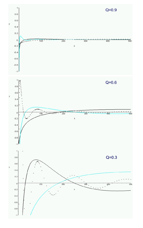
Figure 1: Above we show the deviation from the standard spectrum for different values of $Q$ and $n$. In each plot the dark line corresponds to $n=2$, the light one to $n=3$ and the dotted line to $n=4$. We have set $\alpha_{0}=M_{P}=1$. The effect of the $Q$-deformation is more pronounced in the small $k$ region. Also, the size of the deviation increases significantly as $Q$ approaches $0$.

For power-law inflation the new spectrum has nonstandard dependence on comoving momentum, while the de Sitter spectrum is scale invariant as expected. In both inflationary scenarios the correction to the standard result is characterized by an oscillatory pattern; this modulation has been argued to be a general feature of the ‘minimal’ models described in the introduction. As shown in Fig.(1), the amplitude of the oscillatory pattern is strongly dependent on the deformation parameter. Although only a few values of $Q$ were considered, it is apparent from the plots that the size of the correction increases as $Q$ gets farther away from the classical $Q=1$ limit.

Some of the minimal models Danielsson:2002kx ; Easther:2002xe yield $\frac{H_{0}}{M_{P}}$ corrections, with $H_{0}$ the characteristic Hubble parameter during inflation. When the deformation parameter is very close to its classical value, $Q\sim 1$, the effect of the quantum deformation is of order $\bigl{(}\frac{H_{0}}{M_{P}}\bigr{)}^{2}$, significantly small. However, values of $Q$ close to zero yield a considerable increase in the size of the correction. If in fact $Q$ were small enough to overcome the $\bigl{(}\frac{H_{0}}{M_{P}}\bigr{)}^{2}$ suppression, the effect of the quantum deformation could be measurable in the near future. On the other hand, $Q$ near unity would yield a $\bigl{(}\frac{H_{0}}{M_{P}}\bigr{)}^{2}$ correction to the standard spectrum, most likely impossible to detect.

Since they predict a departure from the standard spectrum of fluctuations, $Q$-deformations can in principle provide us with a window on trans-Planckian physics. Whether the effect can be measured or not, however, depends on the magnitude of the deformation. Regardless, we have shown that $Q$-deformations offer an additional scenario for physics above the Planck scale.

- (1) J. Martin and R. H. Brandenberger, Phys. Rev. D 63, 123501 (2001) [arXiv:hep-th/0005209].
- (2) R. H. Brandenberger and J. Martin, Mod. Phys. Lett. A 16, 999 (2001) [arXiv:astro-ph/0005432].
- (3) G. Amelino-Camelia, Lect. Notes Phys. 541, 1 (2000) [arXiv:gr-qc/9910089].
- (4) J. C. Niemeyer, Phys. Rev. D63, 123502 (2001), [arXiv:astro-ph/0005533]; J. C. Niemeyer, [arXiv:astro-ph/0201511].
- (5) L. Mersini, M. Bastero-Gil and P. Kanti, Phys. Rev. D 64, 043508 (2001) [arXiv:hep-ph/0101210].
- (6) A. A. Starobinsky, Pisma Zh. Eksp. Teor. Fiz. 73, 415 (2001) [JETP Lett. 73, 371 (2001)] [arXiv:astro-ph/0104043].
- (7) R. H. Brandenberger and J. Martin, Int. J. Mod. Phys. A 17, 3663 (2002) [arXiv:hep-th/0202142].
- (8) J. Martin and R. H. Brandenberger, Proceedings of the Ninth Marcel Grossmann Meeting on General Relativity, edited by R. T. Jantzen, V. Gurzadyan and R. Ruffini, World Scientific, Singapore, 2002, [arXiv:astro-ph/0012031].
- (9) J. C. Niemeyer and R. Parentani, Phys. Rev. D64, 101301 (2001), [arXiv:astro-ph/0101451].
- (10) M. Lemoine, M. Lubo, J. Martin and J. P. Uzan, Phys. Rev. D65, 023510 (2002), [arXiv:hep-th/0109128].
- (11) R. H. Brandenberger, S. E. Joras and J. Martin, Phys. Rev. D 66, 083514 (2002), [arXiv:hep-th/0112122].
- (12) A. Kempf, Phys. Rev. D63 (2001) 083514, [arXiv:astro-ph/0009209].
- (13) C. S. Chu, B. R. Greene and G. Shiu, Mod. Phys. Lett. A16, 2231 (2001), [arXiv:hep-th/0011241].
- (14) R. Easther, B. R. Greene, W. H. Kinney and G. Shiu, Phys. Rev. D64, 103502 (2001), [arXiv:hep-th/0104102]; R. Easther, B. R. Greene, W. H. Kinney and G. Shiu, [arXiv:hep-th/0110226].
- (15) A. Kempf and J. C. Niemeyer, Phys. Rev. D64, 103501 (2001), [arXiv:astro-ph/0103225].
- (16) S. F. Hassan and M. S. Sloth, [arXiv:hep-th/0204110].
- (17) F. Lizzi, G. Mangano, G. Miele and M. Peloso, JHEP 0206, 049 (2002), [arXiv:hep-th/0203099].
- (18) R. Brandenberger and P. M. Ho, Phys. Rev. D 66, 023517 (2002), [AAPPS Bull. 12N1, 10 (2002)], [arXiv:hep-th/0203119].
- (19) Q. G. Huang and M. Li, [arXiv:hep-th/0304203].
- (20) U. H. Danielsson, Phys. Rev. D 66, 023511 (2002), [arXiv:hep-th/0203198].
- (21) U. H. Danielsson, JHEP 0207, 040 (2002), [arXiv:hep-th/0205227].
- (22) U. H. Danielsson, JHEP 0212, 025 (2002) [arXiv:hep-th/0210058].
- (23) K. Goldstein and D. A. Lowe, Phys. Rev. D 67, 063502 (2003), [arXiv:hep-th/0208167].
- (24) G. L. Alberghi, R. Casadio and A. Tronconi, [arXiv:gr-qc/0303035].
- (25) C. Armendariz-Picon and E. A. Lim, arXiv:hep-th/0303103.
- (26) N. Kaloper, M. Kleban, A. Lawrence, S. Shenker, [arXiv:/hep-th/0201158].
- (27) R. Easther, B. R. Greene, W. H. Kinney and G. Shiu, Phys. Rev. D 66, 023518 (2002) [arXiv:hep-th/0204129].
- (28) J. C. Niemeyer, R. Parentani and D. Campo, Phys. Rev. D 66, 083510 (2002) [arXiv:hep-th/0206149].
- (29) J. Martin and R. H. Brandenberger, arXiv:hep-th/0305161.
- (30) S. Majid, Int. J. Mod. Phys. A 5, 4689 (1990).
- (31) S. Majid, arXiv:q-alg/9701001.
- (32) J. Teschner, Phys. Lett. B 458, 257 (1999) [arXiv:hep-th/9902189].
- (33) V. F. Mukhanov, H. A. Feldman and R. H. Brandenberger, Phys. Rept. 215, 203 (1992).
- (34) A. Jevicki and S. Ramgoolam, JHEP 9904, 032 (1999) [arXiv:hep-th/9902059].
- (35) E. Mottola, Phys. Rev. D 31, 754 (1985).
- (36) B. Allen, Phys. Rev. D 32, 3136 (1985).