Abstract

The behavior of solitons in integrable theories is strongly constrained by the integrability of the theory, that is by the existence of an infinite number of conserved quantities that these theories are known to possess. As a result the soliton scattering of such theories are expected to be trivial (with no change of direction, velocity or shape). In this paper we present an extended review on soliton scattering of two spatial dimensional integrable systems which have been derived as dimensional reductions of the self-dual Yang-Mills-Higgs equations and whose scattering properties are highly non-trivial.

1 Introduction

Solitons which scatter in a non-trivial way and which occur as solutions of planar integrable systems are going to be presented. Initially solitons were introduced by mathematicians to describe lumps of energy stable to perturbations which do not change either their velocity or their shape when colliding with each other. They have been observed experimentally both as waves on shallow water and in laser pulses in fibre-optic cables, among other places. Solitons also play an important role in various models of subatomic particles (quantum field theories). In recent literature all sorts of localized energy configurations have been called solitons which travel without assuming stability of the shape or velocity or a simple behavior in collision.

In one space dimension integrable systems occur when dispersion effects are exactly balance by nonlinearities. However, in more than one dimensions the definition of an integrable model is related with the existence of infinite number of conserved quantities; of Painlevé property; of two linear equations (so-called the Lax pair) which compatibility condition give the non-linear soliton equation; of inverse-scattering transform; even of multi-soliton solutions (see, for example, [1]).

An interesting problem is the investigation of the scattering properties of two or more solitons colliding. In some known models with non-trivial topology the collision of two solitons is inelastic (some radiation is emitted) and non-trivial, ie a head-on collision results in $90^{0}$ scattering (see, for example, [2] and references therein). On the other hand, the solitons of integrable models interact trivially in the sense that they pass through each other with no lasting change in velocity, shape or direction. Some examples in 2+1 dimensions are the Kadomtsev-Petviashvili [3], the Konopelchenko-Rogers [4], the Davey-Stewrtson [5] and the integrable chiral equation [6]. Until recently, non-trivial scattering of solitons occurs mostly in non-integrable models which is far from simple. The issue discussed here is whether such type of scattering can occur in integrable models too. There are some limited examples of integrable models where soliton dynamics is non-trivial. In 1+1 dimensions there are many models that non-trivial soliton-like solutions (cf. Ref. [7]) exists like the boomeron solutions [8] which are solitons with time-dependent velocities. In 2+1 dimensions there are the dromion solutions [9] of the Davey-Stewartson equation which decay exponentially in both spatial coordinates and interact in a non-trivial matter [10] and the soliton solutions of the Kadomtsev-Petciashvilli equations whose scattering properties are highly non-trivial [11].

Recently in [12]-[14] families of soliton solutions have been constructed for planar integrable systems (using analytical methods) with different types of scattering behavior. This happens since the solitons of the systems have internal degrees of freedom that although they determine their space orientation, they do not change the energy density and they are important in understanding the system evolution. Therefore, solitons can interact either trivially or non-trivially depending on the orientation of these internal parameters and on the values of the impact parameters defined as the distance of closest of approach between their centers in the absence of interaction.

In what follows we will review the approach based on the Riemann-Hiblert problem with zeros, first presented in [12]-[14], in order to construct soliton solutions with non-trivial scattering for two spatial dimensional integrable models defined in anti-de Sitter and Minkowski space, respectively. Both models are equivalent to the self-dual Yang-Mills-Higgs equations reduced from 2+2 to 2+1 dimensions while the soliton solutions are related to hyperbolic and Euclidean Bogomolny-Prasad-Sommerfield (BPS) monopoles.

2 Self-dual Yang-Mills-Higgs Equations

Static BPS monopoles are solutions of non-linear elliptic partial differential equations on some three-dimensional Riemannian manifold. Most work on monopoles has dealt with the case when this manifold is the Euclidean space $\hbox{\upright\hbox to0.0pt{I\hss}\kern 1.7ptR}^{3}$ since then the equations are integrable and sophisticated geometrical techniques like twistor theory can be applied. Note that the introduction of time-dependence destroys the integrability. In addition, the monopole equations on hyperbolic space $\mbox{\hbox{\upright\hbox to0.0pt{I\hss}\kern 1.7ptH}}^{3}$ are also integrable [15] and often hyperbolic monopoles turn out to be easier to study than the Euclidean ones as first studied by Atiyah and explicitly shown in [16]. In fact as it has been rigorously established in [17], in the limit as the curvature of hyperbolic space tends to zero the Euclidean monopoles are recovered.

Let us first consider an integrable system [18] which is related to hyperbolic monopoles and which is obtained from replacing the positive definite hyperbolic space $\mbox{\hbox{\upright\hbox to0.0pt{I\hss}\kern 1.7ptH}}^{3}$ by a Lorentzian version, the so-called anti-de Sitter space. Thus, the self-dual Yang-Mills-Higgs equations are of the form

$$D_{i}\Phi=\frac{1}{2\sqrt{|g|}}g_{ij}\,\varepsilon^{jkl}F_{kl}$$ (1)

where the Yang-Mills-Higgs fields take values on a three-dimensional Riemannian manifold (${\cal M}$) with gauge group $SU(2)$. In particular, $A_{k}$ (for $k=0,1,2$) is the $su(2)$-valued gauge potential, $F_{ij}=\partial_{i}A_{j}-\partial_{j}A_{i}+[A_{i},A_{j}]$ is the field strength and $\Phi=\Phi(x^{\mu})$ is the $su(2)$-valued Higgs field; while $x^{\mu}=(x^{0},x^{1},x^{2})$ represent the local coordinates on ${\cal M}$. The action of the covariant derivative $D_{i}=\partial_{i}+A_{i}$ on $\Phi$ is: $D_{i}\Phi=\partial_{i}\Phi+[A_{i},\Phi]$. Equation (1) for constant curvature is integrable in the sense that a Lax pair exists.

Note that the solutions of (1) which can be described in terms of holomorphic vector bundles or in terms of rational functions correspond to Euclidean or hyperbolic BPS monopoles when $({\cal M},g)$ is the Euclidean $\hbox{\upright\hbox to0.0pt{I\hss}\kern 1.7ptR}^{3}$ or the hyperbolic $\mbox{\hbox{\upright\hbox to0.0pt{I\hss}\kern 1.7ptH}}^{3}$ space, respectively. Also, both of the models presented here can be obtained from (1) as dimensional reductions of the four-dimensional self-dual Yang-Mills-Higgs equations for appropriate gauge choices [1].

3 The Anti-de Sitter Model

Currently a great deal of attention has been focused on anti-de Sitter spaces since they arise naturally in black holes and $p$-branes. For the case of Yang-Mills theory with ${\cal N}=4$ supersymmetries and a large number of colors it has been conjectured that gauge strings are the same as the fundamental strings but moving in a particular curved space: the product of five-dimensional anti-de Sitter space and a five sphere [19]. Then, using Poincaré coordinates the anti-de Sitter solutions play the role of classical sources for the boundary field correlators, as shown in [20]; while extensions of the corresponding statements can be applied to gravity theories, like black holes which arise in anti-de Sitter backgrounds.

By definition the (2+1)-dimensional anti-de Sitter space is the universal covering space of the hyperboloid ${\cal H}$ defined by the equation

$$U^{2}+V^{2}-X^{2}-Y^{2}=1$$ (2)

with metric

$$ds^{2}=-dU^{2}-dV^{2}+dX^{2}+dY^{2}.$$ (3)

By parametrizing the hyperboloid ${\cal H}$ by

$$U = \sec\rho\cos\theta$$

$$V = \sec\rho\sin\theta$$

$$X = \tan\rho\cos\phi$$

$$Y = \tan\rho\sin\phi$$ (4)

for $\rho\in[0,\pi/2)$, the corresponding metric simplifies to

$$ds^{2}=\sec^{2}\rho\left(-d\theta^{2}+d\rho^{2}+\sin^{2}\rho\,d\phi^{2}\right).$$ (5)

The spacetime contains closed timelike curves due to the periodicity of $\theta$ [21]. In fact $(\rho,\phi)$ correspond to polar coordinates and $\theta\in R$ being the time; while anti-de Sitter space (as a manifold) is the product of an open spatial disc with $\theta$ and curvature equal to minus six. Null spacelike infinity ${\cal I}$ consists of the timelike cylinder $\rho=\pi/2$ and this surface is never reached by timelike geodesics.

If the Poincaré coordinates $(r,x,t)$ for $r>0$ are defined as

$$r = \frac{1}{U+X}$$

$$x = \frac{Y}{U+X}$$

$$t = \frac{-V}{U+X}$$ (6)

the metric simplifies to the following form

$$ds^{2}=r^{-2}(-dt^{2}+dr^{2}+dx^{2}).$$ (7)

Note that the Poincaré coordinates cover a small part of anti-de Sitter space which correspond to half of the hyperboloid ${\cal H}$ for $U+X>0$ as shown in Figure 1. The surface $r=0$ is part of infinity ${\cal I}$.

Figure 1: The Penrose diagram of anti-de Sitter space. The boundary of anti-de Sitter is the boundary of the cylinder.

Consider the set of linear equations

$$\left[rD_{r}-2(\lambda-u)D_{u}-\Phi\right]\Psi = 0$$

$$\left[2D_{v}+\frac{\lambda-u}{r}D_{r}-\frac{\lambda-u}{r^{2}}\Phi\right]\Psi = 0.$$ (8)

Here $\lambda\in{\hbox to0.0pt{\hbox to0.0pt{C\hss}\kern 3.8pt\vrule height=8.0pt,width=0.4pt,depth=-0.1pt\hss}\phantom{C}}$ and $(r,u,v)$ are the Poincaré coordinates (where $u=x+t$ and $v=x-t$) while the gauge fields $(\Phi,A_{r},A_{u},A_{v})$ are $2\times 2$ trace-free matrices depending only on $(r,u,v)$ and $\Psi(\lambda,r,u,t)$ is a unimodular $2\times 2$ matrix function satisfying the reality condition $\Psi(\lambda)\Psi(\bar{\lambda})^{\dagger}=I$ (where $\dagger$ denotes the complex conjugate transpose). The system (8) is overdetermined and in order for a solution $\Psi$ to exist the following integrability conditions need to be satisfied

$$D_{u}\Phi = rF_{ur}$$

$$D_{v}\Phi = -rF_{vr}$$

$$D_{r}\Phi = -2rF_{uv}$$ (9)

which correspond to the self-dual Yang-Mills-Higgs equations (1) defined in the 2+1 anti-de Sitter space. The gauge and Higgs fields in terms of the function $\Psi$ can be obtained from the Lax pair (8) due to the boundary conditions. Note that, as $\lambda\rightarrow\infty$ the function $\Psi$ goes to the identity matrix and the system (8) implies that

$$A_{u}=0,\hskip 14.22636pt\hskip 14.22636ptA_{r}=\frac{1}{r}\,\Phi.$$ (10)

On the other hand, for $\lambda=0$ and using (10) the rest of the gauge fields are defined as

$$\Phi = -\frac{r}{2}\,J_{r}J^{-1}-u\,J_{u}J^{-1}$$

$$A_{v} = \frac{u}{2r}\,J_{r}J^{-1}-J_{v}J^{-1}$$ (11)

where $J(r,u,v)\doteq\Psi(\lambda=0,r,u,v)$. As a result the first equation of the system (9) is automatically satisfied (due to the specific gauge choice).

Recently, Ward [18] has shown that holomorphic vector bundles $V$ over $Q$ determine multi-soliton solutions of (9) in anti-de Sitter space via the usual Penrose transform. This way a five-parameter family of soliton solutions can be obtained, in a similar way as for flat spacetime [22]. Later, more solutions of equations (9) were obtained by Zhou [23, 24] using Darboux transformations with constant and variable spectral parameter. In what follows, we use the Riemann problem with zeros to construct families of soliton solutions and observe the occurrence of different types of scattering behavior. More precisely, we present families of multi-soliton solutions with trivial and non-trivial scattering.

3.1 Baby Monopoles

In this section, we illustrate the construction of time-dependent solutions related to hyperbolic monopoles. In particular, families of soliton solutions of the self-dual Yang-Mills-Higgs equations defined in the (2+1)-dimensional anti-de Sitter space are constructed and their dynamics is studied in some detail.

The integrable nature of (1) means that there is a variety of methods for constructing solutions. Here, we indicate a general method for constructing soliton solutions of (9) which is a variant of that presented in Ref. [22]. Using the standard method of Riemann problem with zeros, in order to construct the multi-soliton solutions, we assume that the function $\Psi$ of the system (8) has the simple form in $\lambda$

$$\Psi=I+\sum_{k=1}^{n}\frac{M_{k}}{\lambda-\mu_{k}}$$ (12)

where $M_{k}$ are $2\times 2$ matrices independent of $\lambda$ and $n$ corresponds to the soliton number. The components of the matrix $M_{k}$ are given in terms of a rational function $f_{k}(\omega_{k})=a_{k}\,\omega_{k}+c_{k}$ of the complex variable: $\omega_{k}=v-r^{2}\,(\mu_{k}-u)^{-1}$. Here $a_{k}$, $c_{k}$ and $\mu_{k}$ are complex constants which determine the size, position and velocity of the $k$-th solitons. Remark: The rational dependence of the solutions $\Psi$ follows (directly) when the inverse spectral theory is considered. In fact in [25] (for flat spacetime), it was shown from the Cauchy problem that the spectral data is a function of a parameter similar to $\omega_{k}$.

By considering the unitarity condition of the eigenfunction $\Psi$ and keeping in mind that the gauge fields are independent of the spectral parameter $\lambda$ it can be shown that the matrix $M_{k}$ has the form

$$M_{k}=\sum_{l=1}^{n}(\Gamma^{-1})^{kl}\bar{m}_{a}^{l}m_{b}^{k}$$ (13)

with $\Gamma^{-1}$ the inverse of

$$\Gamma^{kl}=\sum_{a=1}^{2}(\bar{\mu}_{k}-\mu_{l})^{-1}\bar{m}_{a}^{k}m_{a}^{l}$$ (14)

and $m^{k}_{a}$ holomorphic functions of $\omega_{k}$ of the form $m^{k}_{a}=(m_{1}^{k},m_{2}^{k})=(1,f_{k})$. The Yang-Mills-Higgs fields $(\Phi,A_{r},A_{v},A_{u})$ can then be read off from (10-11) and they automatically satisfy (9) while the corresponding solitons are spatially localized since $\Phi\rightarrow 0$ at spatial infinity.

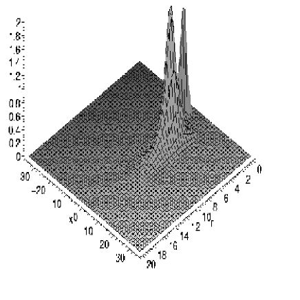
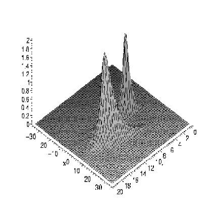
Figure 2: A two-soliton configuration with trivial scattering at different times.

By way of example, let us look at the special case where $\mu_{1}=1+i$, $\mu_{2}=2i$, $a_{1}=2$, $a_{2}=1$, $c_{1}=5$ and $c_{2}=-10$. Figure 2 represents snapshots of the positive definite gauge quantity ($-\mbox{tr}\Phi^{2}$) at different times. The corresponding solution consists of two solitons which travel towards infinity ($r=0$) and bounce back while their sizes change as they move.

Note that the Riemann problem with zeros method was first introduced by Zakharov and his collaborators [26] in his pioneer work of applying spectral theory to generate soliton solutions of integrable equations. Later this approach has been applied to obtain the monopole solutions of the four-dimensional self-dual Yang-Mills-Higgs equations [27]. However, as it can been observed from (12), the Riemann problem with zeros method assumes that the parameters $\mu_{k}$ are distinct and also $\bar{\mu}_{k}\neq\mu_{l}$ for all $(k,l)$. In what follows examples are given of two generalizations of these constructions: one involving higher-order poles in $\mu_{k}$ and the other where $\bar{\mu}_{k}=\mu_{l}$.

$\diamondsuit$  High-order poles in $\mu_{k}$

Firstly, let us look at an example in which the function $\Psi$ has a double pole in $\lambda$ and no others. In this case, $\Psi$ has the form

$$\Psi=I+\sum_{k=1}^{2}\frac{R_{k}}{(\lambda-\mu)^{k}}$$ (15)

where $R_{k}$ are $2\times 2$ matrices independent of $\lambda$. Then $\Psi$ corresponds to a solution of (8) if and only if it factorizes as [14]

$$\Psi(\lambda)\!=\!\left(1-\frac{\bar{\mu}-\mu}{(\lambda-\mu)}\frac{q^{\dagger}\otimes q}{|q|^{2}}\right)\!\left(1\!-\!\frac{\bar{\mu}-\mu}{(\lambda-\mu)}\frac{p^{\dagger}\otimes p}{|p|^{2}}\right)$$ (16)

for some two vectors $q$ and $p$. One way to derive the structure of these vectors is to take the formula (12) for $n=2$, set $\mu_{1}=\mu+\varepsilon$, $\mu_{2}=\mu-\varepsilon$ and $f_{1}(\omega_{1})=f(\omega_{1})+\varepsilon h(\omega_{1})$, $f_{2}(\omega_{2})=f(\omega_{2})-\varepsilon h(\omega_{2})$, with $f$ and $h$ being rational function of one variable. In the limit $\varepsilon\rightarrow 0$ the two vectors $q$ and $p$ can be obtained and are of the form:

$$q = (1+|f|^{2})(1,f)+(\bar{\mu}-\mu)\!\left(\frac{r^{2}\,f^{\prime}}{(\mu-u)^{2}}+h\!\right)(\bar{f},-1),$$

$$p = (1,f)$$ (17)

where $f$ and $h$ are rational functions of $\omega=v-r^{2}(\mu-u)^{-1}$ while $f^{\prime}$ denotes the derivative of $f$ with respect to its argument. In this case, the solution depends on the parameter $\mu$ and on the two arbitrary functions $f$ and $h$. Note that the constraint $f_{2}(\omega_{2})-f_{1}(\omega_{1})\rightarrow 0$ as $\varepsilon\rightarrow 0$ has to be imposed in order for the resulting solution $\Psi$ to be smooth for all $(r,u,v)$ which is the case here.

In order to illustrate the above family of solutions two simple cases are going to be examined by giving specific values to the parameters $\mu$, $f(\omega)$ and $h(\omega)$.

• Let us study the simple case where $\mu=i$, $f(\omega)=\omega$ and $h(\omega)=0$. Then, the quantity $-\mbox{tr}\Phi^{2}$ simplifies to

  $$-\mbox{tr}\Phi^{2}=32r^{2}\frac{\left((r^{2}+x^{2}\!-\!t^{2}\!+\!1)^{2}+4t^{2}\right)\left((r^{2}+x^{2}\!-\!t^{2}\!-\!1)^{2}+4x^{2}\right)}{\left[\left((r^{2}+x^{2}-t^{2})^{2}+1+2t^{2}+2x^{2}\right)^{2}+4r^{4}\right]^{2}}$$ (18)

  which is time reversible. The corresponding time-dependent solution is a travelling ring-like soliton configuration which for negative $t$, goes towards spatial infinity $(r=0)$; approaches it at $t=0$ and then bounces back at positive $t$ while the soliton size deforms, as shown in Figure 3. Ring structures occur in the soliton scattering of many non-integrable planar systems and are approximations of multi-solitons [28].

  

  

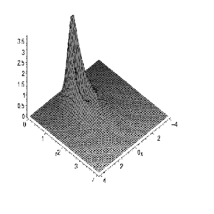
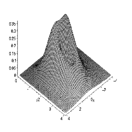
  Figure 3: A stationary soliton configuration at different times.

  

  

  

  

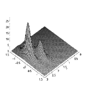
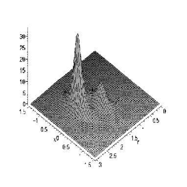
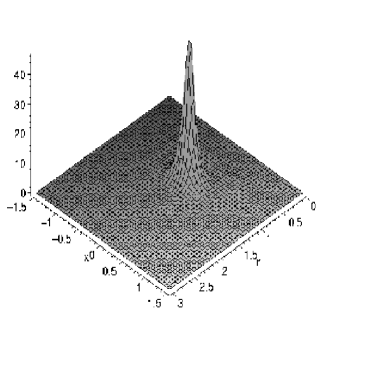
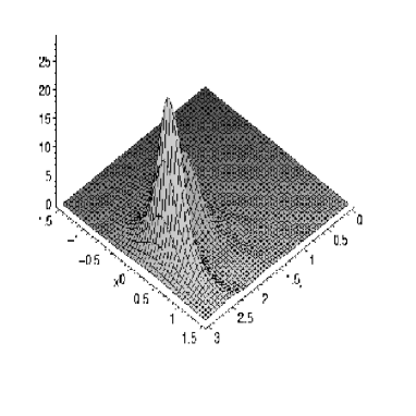
  Figure 4: A non-trivial dynamics of two solitons in anti-de Sitter space.

• Next, we investigate the solution which corresponds to a non-trivial soliton scattering as presented in Figure 4. The solution has been obtained by (16-17) for the following values of the parameters: $\mu=i$, $f(\omega)=\omega$ and $h(\omega)=\omega^{4}$ while the picture consists of two different-sized solitons. For large (negative) $t$, the gauge quantity $-\mbox{tr}\Phi^{2}$ is peaked at two points, forms a lump at $t=0$ and then two solitons emerge, for large (positive) $t$, with the small one been shifted to the left.

These solutions can also been obtained using Uhlenbeck’s construction [29]. In this approach the function $\Psi$ is assumed to be a product of factors which when substituted in the Lax pair (8) the problem simplifies to finding solutions of simple first-order partial differential equations [30]. Both methods can be extended to derive solutions where the function $\Psi$ has higher order pole in $\lambda$ (and no others). Then, $\Psi$ can be written as a product of three (or more) factors with three (or more) arbitrary vectors (for more details, see [13]).

$\diamondsuit$  Case where $\bar{\mu}_{k}=\mu_{l}$

Secondly, let us construct a large family of solutions which correspond to the case where $\bar{\mu}_{k}=\mu_{l}$. One way of proceeding is to take the solution $(\ref{Psi})$ with $n=2$, put $\mu_{1}=\mu+\varepsilon$, $\mu_{2}=\bar{\mu}-\varepsilon$ and take the limit $\varepsilon\rightarrow 0$. In order for the resulting $\Psi$ to be smooth it is necessary to take $f_{1}(\omega_{1})=f(\omega_{1})$, $f_{2}(\omega_{2})=-1/f(\omega_{2})-\varepsilon h(\omega_{2})$ where $f$ and $h$ are rational functions of one variable. On taking the limit we obtain a solution $\Psi$ of the form

$$\Psi=I+\frac{n^{1}\otimes m^{1}}{\lambda-\mu}+\frac{n^{2}\otimes m^{2}}{\lambda-\bar{\mu}}$$ (19)

where $n^{k}$, $m^{k}$ for $k=1,2$ are complex valued two vector functions of the form

$$\hskip-34.14322ptm^{1}=(1,f),\hskip 14.22636ptm^{2}=(-\bar{f},1)$$

$$\hskip 0.0pt\pmatrix{\!n^{1}\cr n^{2}\!}\!\! = \!\!\frac{2(\mu-\bar{\mu})}{4(1\!+\!|f|^{2})^{2}\!-\!(\mu\!-\!\bar{\mu})^{2}|w|^{2}}\!\!\pmatrix{\!2(1\!+\!|f|^{2})\!&\!-(\mu\!-\!\bar{\mu})\bar{w}\cr\!\!(\mu\!-\!\bar{\mu})w\!&\!-2(1\!+\!|f|^{2})\!}\pmatrix{\!m^{1\dagger}\cr m^{2\dagger}\!}$$ (20)

with

$$w\equiv\frac{2r^{2}}{(\mu-u)^{2}}f^{\prime}+\bar{h}f^{2}.$$ (21)

So we generate a solution which depends on the parameter $\mu$ and the two arbitrary rational functions $f=f(\omega)$ and $h=h(\bar{\omega})$.

In Figure 5 we represent snapshots of the solution (19) for $\mu=i$, $f=\omega$ and $h=\bar{\omega}$. The configuration consists of two solitons with non-trivial scattering behavior. Again, the quantity $-\mbox{tr}\Phi^{2}$ is peaked at two points, for (negative) $t$, which are still distinct at $t=0$ and then two shifted (compared to the initial ones at $t=-2.5$) solitons emerge, for (positive) $t$. Throughout the time-evolution their sizes change. Note that, the scattering solutions belong to a large family since $f$ and $h$ can be taken to be any rational functions of $\omega$.

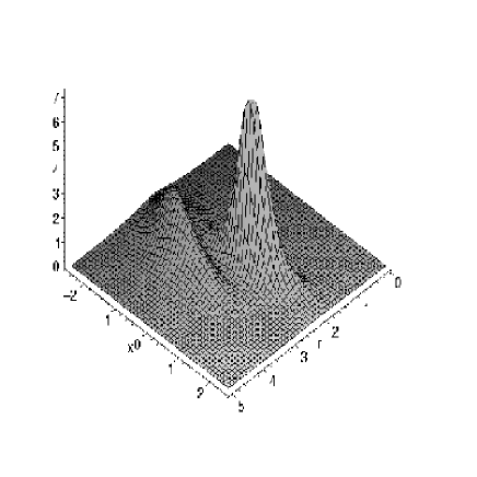
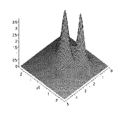
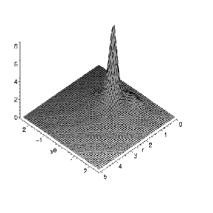
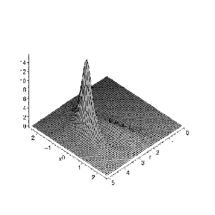
Figure 5: A non-trivial dynamics of two solitons in anti-de Sitter space.

Remark: The extension of the obtained classical solutions in the whole anti-de Sitter space, ie using the coordinates $(\rho,\theta,\phi)$, is unambiguous. For example, the simplest solution which corresponds to the one soliton (first derived in [18]) given by (12) for $n=1$, $\mu_{1}=i$ and $f_{1}=\omega_{1}$ implies that

$$-\mbox{tr}\,\Phi^{2} = \frac{8r^{4}}{[(r^{2}+x^{2}-t^{2})^{2}+2x^{2}+2t^{2}+1]^{2}}$$ (22)

$$= \frac{2\cos^{4}\rho}{(\cos^{2}\rho-2)^{2}}$$

which means that the positive definite quantity $-\mbox{tr}\,\Phi^{2}$ is independent of the variables $(\theta,\phi)$.

4 The Minkowski Model

The integrable $SU(2)$ chiral model introduced by Ward [6] is described by the field equation

$$\partial_{v}\left(J^{-1}\partial_{u}J\right)-\partial_{x}\left(J^{-1}\partial_{x}J\right)=0$$ (23)

where the chiral field takes values in: $J\in SU(2)$ while $u=\frac{1}{2}(t+y)$ and $v=\frac{1}{2}(t-y)$. Note that the integrable chiral equation is related to the Jarvis equation studied in [16]. Once more the equation can be obtained from the self-dual Yang-Mills-Higgs equation given by (1) for specific gauge choice (further details in [31]). Then for specific boundary conditions spherical symmetric monopole solutions could be derived using the harmonic map ansatz as studied in [16].

Here the choice of the boundary conditions follows from the chiral-equation form rather than the gauge-theory form, ie

$$J=J_{0}+\frac{1}{r}J_{1}(\theta)+O\left(\frac{1}{r^{2}}\right),\hskip 14.22636ptr\rightarrow\infty$$ (24)

for $x+iy=re^{i\theta}$. Here $J_{0}$ is a constant matrix and $J_{1}$ depends only on $\theta$ (no time dependence).

The model possess a conserved energy density given by [6]

$${\cal E}=-\frac{1}{2}\mbox{tr}\left(\left(J^{-1}\partial_{t}J\right)^{2}+\left(J^{-1}\partial_{x}J\right)^{2}+\left(J^{-1}\partial_{y}J\right)^{2}\right)$$ (25)

which is a positive-defined functional of the chiral field.

The integrable equation (23) can be written as the compatibility condition of the system

$$\left(\lambda\partial_{x}-\partial_{u}\right)\psi = A\psi$$

$$\left(\lambda\partial_{v}-\partial_{x}\right)\psi = B\psi$$ (26)

where $\lambda\in{\hbox to0.0pt{\hbox to0.0pt{C\hss}\kern 3.8pt\vrule height=8.0pt,width=0.4pt,depth=-0.1pt\hss}\phantom{C}}$, $A,B$ are $2\times 2$ anti-Hermitian trace-free matrices depending only on $(u,v,x)$ and $\psi(\lambda,u,v,x)$ is an unimodular $2\times 2$ matrix satisfying the reality condition: $\psi(\lambda)\psi(\bar{\lambda})^{\dagger}=I$. The gauge choice of the matrices $A,B$ can be obtained by setting for $\lambda=0$: $\psi(\lambda=0)=J(u,v,x)^{-1}$. Then the system (26) implies that

$$A=J^{-1}\partial_{u}J,\hskip 14.22636pt\hskip 14.22636pt\hskip 14.22636pt\hskip 14.22636ptB=J^{-1}\partial_{x}J.$$ (27)

Using the standard method of Riemann-Hilbert problem with zeros, Ward [6] was able to construct the multi-soliton solutions of (23) by assuming that $\psi$ has a simple poles in $\lambda$ and no others, ie:

$$\psi=I+\sum_{k=1}^{n}\frac{M_{k}}{\lambda-\mu_{k}}$$ (28)

where $M_{k}$ are $2\times 2$ matrices independent of the spectral parameter $\lambda$ given by (13-14), $n$ is the soliton number and the complex parameter $\mu_{k}$ defines the velocity of the $k$-th soliton. Note that the construction is similar to the construction of baby monopoles presented in section 3.1. Again, here the components of $M_{k}$ are given in terms of a rational function $f_{k}$ of the complex variable $\omega_{k}=x+\mu_{k}u+\mu_{k}^{-1}v$. In particular $m_{\alpha}^{k}$ are holomorphic function of $\omega_{k}$ defined as: $m_{\alpha}^{k}=(m_{1}^{k},m_{2}^{k})=(1,f_{k})$. By letting $f_{k}$ to be exponential functions of $\omega_{k}$ the solutions correspond to extended waves which suffer a phase shift upon scattering studied in [32]. In general though, by letting $f_{k}$ to be any rational function of $\omega_{k}$ the corresponding soliton dynamics is trivial with no change of direction or phase shift.

Remark: In [25] it was shown that when the spectral theory was applied for (23) the eigenfunction satisfies a local Riemann-Hilbert problem given by:

$$\psi^{-}=\psi^{+}\left(I-S(x+\lambda u+\lambda^{-1}v)\right).$$ (29)

and the pure soliton solutions can be obtained by letting $\lambda=\bar{\mu}_{l}$ in (28) while the components of the $M_{k}$ matrix can be obtained by solving simple algebraic matrix equations.

4.1 Non-trivial Soliton Scattering

Here we present the way to obtain solitons with non-trivial scattering properties, similar to the anti-de Sitter ones. Note that since the space is flat the non-trivial scattering can be observed and studied in a more clear way. Once more, we concentrate in cases where the formula (28) is not well-defined: ie when $\mu_{k}$ are not distinct or when $\bar{\mu}_{k}=\mu_{l}$ for any $(k,l)$.

$\diamondsuit$ $\pi/N$ Scattering

Assume that $\psi$ has a double pole in $\lambda$ and no others:

$$\psi=I+\sum^{2}_{k=1}\frac{R_{k}}{(\lambda-\mu)^{k}}$$ (30)

where $R_{k}$ are $2\times 2$ matrices independent of $\lambda$. This hypothesis can be generalized by taking $\psi$ to have a pole of order $n$ in $\lambda$ (for more details see [13]). Then $\psi$ satisfies the reality condition if and only if is factorized as [12]

$$\psi(\lambda)=\left(I-\frac{(\bar{\mu}-\mu)}{(\lambda-\mu)}\frac{q_{1}^{\dagger}\otimes q_{1}}{|q|^{2}}\right)\left(I-\frac{(\bar{\mu}-\mu)}{(\lambda-\mu)}\frac{q_{2}^{\dagger}\otimes q_{2}}{|q|^{2}}\right)$$ (31)

where $q_{i}$ for $i=1,2$ are two-dimensional vectors of the form:

$$q_{1} = \left(1+|f|^{2}\right)\left(1,f\right)+{\cal\theta}\left(\bar{\mu}-\mu\right)\left(\bar{f},-1\right)$$

$$q_{2} = \left(1,f\right).$$ (32)

Here $f$ is a rational function of $\omega=x+\mu u+\mu^{-1}v$ and ${\cal\theta}=\left(u-\mu^{-2}v\right)f^{\prime}(\omega)+h(\omega)$. So the solution corresponds to a large family since one may take $f$ and $h$ to be any rational meromorphic functions of $\omega$. Then the chiral field defined as: $J=\psi(\lambda=0)^{-1}$ which takes the product form

$$J=\left(I+\frac{(\bar{\mu}-\mu)}{\mu}\frac{q_{2}^{\dagger}\otimes q_{2}}{|q|^{2}}\right)\left(I+\frac{(\bar{\mu}-\mu)}{\mu}\frac{q_{1}^{\dagger}\otimes q_{1}}{|q|^{2}}\right)$$ (33)

is smooth on $\hbox{\upright\hbox to0.0pt{I\hss}\kern 1.7ptR}^{2+1}$ (since the vectors $q_{i}$ are nowhere zero) and satisfies the boundary condition irrespectively of the choice of $f$ and $h$.

The solution (31) has been obtained as a limit of the simple-pole case (30) with $n=2$. The idea is to take the limit $\mu_{k}\rightarrow\mu$ by setting $\mu_{1}=\mu+\varepsilon$, $\mu_{2}=\mu-\varepsilon$ which implies that the corresponding functions take the form $f_{1}(\omega_{1})=f(\omega_{1})+\varepsilon h(\omega_{1})$ and $f_{2}(\omega_{2})=f(\omega_{2})-\varepsilon h(\omega_{2})$. Note that in the limit $\varepsilon\rightarrow 0$ then $f_{2}(\omega_{2})-f_{1}(\omega_{1})\rightarrow 0$ which results the smoothness of $\psi$. The corresponding solitons are located when the chiral field $J$ departs from its asymptotic value $J_{0}$ which occurs when $\theta\rightarrow 0$.

In principal, it is possible to visualize the emerging soliton structures when the functions $f$ and $h$ are rational functions of degree $p,q\in\hbox{\upright\hbox to0.0pt{I\hss}\kern 1.7ptN}$ of the form: $f(\omega)=\omega^{p}$ and $h(\omega)=\omega^{q}$. In fact, for $q>p$ the configuration consists of $p-1$ static solitons located at the center-of-mass of the system forming a ring-like structure if more than one; accompanied by $N=q-p+1$ solitons which (initially) accelerate towards the one in the middle, scatter at an angle of $\pi/N$ and (finally) decelerate as they separate. This follows from the following analytic argument: the field $J$ departs from its asymptotic value $J_{0}$ when $\theta=\omega^{p-1}\left(p\left(u-\mu^{-2}v\right)+\omega^{N}\right)\rightarrow 0$ which holds when either $\omega^{p-1}=0$ or $\omega^{N}+p\left(u-\mu^{-2}v\right)=0$. These are approximately the locations of the solitons in the $xy$-plane.

Let us illustrate the above family of soliton solutions by examining two simple cases by giving specific values to the arbitrary parameters $\mu,f(\omega)$ and $h(\omega)$.

• Let us investigate the simple case where $\mu=i$, $f(\omega)=\omega$ and $h(\omega)=0$. Then the corresponding energy density takes the simple form

  $${\cal E}=16\frac{r^{4}+2r^{2}+4t^{2}(2r^{2}+1)+1}{\left(r^{4}+2r^{2}+4t^{2}+1\right)^{2}}$$ (34)

  where $r$ is the polar coordinate: $r=\sqrt{x^{2}+y^{2}}$ while the energy density is time reversible. Figure 6 presents snapshots of the stationary soliton configuration which forms a single peak at $t=0$ and expands to a ring as $t$ increases. For large positive $t$, the height of the ring (ie maximum of ${\cal E}$) is proportional to $t^{-1}$ while its radius is proportional to $\sqrt{t}$.

  

  

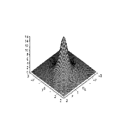
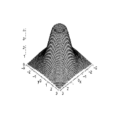
  Figure 6: A stationary soliton configuration at different times in flat spacetime.

  

  

  

  

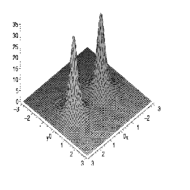
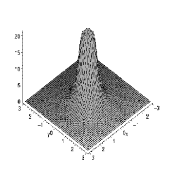
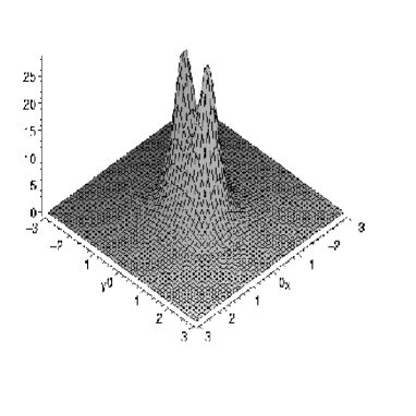
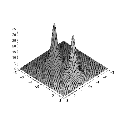
  Figure 7: A $90^{0}$ scattering of two soliton in flat spacetime.

• Next let us take $\mu=i$, $f(\omega)=\omega$ and $h(\omega)=\omega$. The energy density is given by

  $${\cal E}=16\frac{5r^{4}+10r^{2}+4t^{2}(1+2r^{2})-8t(x^{2}-y^{2})+1}{\left(5r^{4}+2r^{2}+4t^{2}+8t(x^{2}-y^{2})+1\right)^{2}}$$ (35)

  and is symmetric under the interchange $t\rightarrow-t,x\rightarrow y,y\rightarrow x$. Figure 7 presents the collision of two solitons near $t=0$: the solitons accelerate towards each other, scatter at right angles and decelerate as they separate. In particular, the collision is time symmetric and elastic (no emitted radiation).

  Note that for negative $t$, the two solitons (following the asymptotic argument of $J$) are located on the $x$-axis at $x\approx\pm\sqrt{t}$ while for positive $t$, they are located in the $y$-axis at $y\approx\pm\sqrt{-t}$. Once more the corresponding solitons are not of constant size: their height is proportional to $t^{-1}$ while their radii are proportional to $\sqrt{t}$. In fact the solitons spread out as they move apart.

Although it seems strange that by taking the limit of soliton solutions with trivial scattering soliton solutions with non-trivial scattering have been obtained there is an explanation as shown in [13]. By studying the effect of the variation of $\varepsilon$ to a two soliton configuration it has been observed that at the limit $\varepsilon\rightarrow 0$ the solitons disperse, shift and interact with each other since their internal degrees of freedom and their impact parameter change. As a result the two initial well-separated solitons form a ring at the limit $\varepsilon\rightarrow 0$.

In general in a head-on collision of $N$ indistinguishable solitons the scattering angle of the emerging structures relative to the incoming ones can be $\pi/N$. In particular when the $N$ solitons are very close together they merge and form a ring-like structure and finally they emerge from the ring in a direction that bisects the angle formed by the incoming ones.

$\diamondsuit$ Elastic soliton-antisoliton non-trivial scattering

Next we construct a large family of solutions which represent soliton-antisoliton field configurations [13]. The corresponding solution has the form

$$\psi(\lambda)=I+\frac{n^{1}\otimes m^{1}}{\lambda-i}+\frac{n^{2}\otimes m^{2}}{\lambda+i}$$ (36)

where $n^{k},m^{k}$ (for $k=1,2$) are complex-valued two-dimensional vectors independent of $\lambda$ of the form:

$$m^{1} = (1,f),\hskip 14.22636pt\hskip 14.22636ptm^{2}=(-\bar{f},1)$$

$$\pmatrix{n^{1}\cr n^{2}}\!\! = \!\!\frac{1}{\left(1+|f|^{2}\right)^{2}+|w|^{2}}\pmatrix{2i\left(1+|f|^{2}\right)&2\bar{w}\cr-2w&-2i\left(1+|f|^{2}\right)}\pmatrix{m^{1\dagger}\cr m^{2\dagger}}$$ (37)

with

$$w=\bar{h}f^{2}+2tf^{\prime}.$$ (38)

So we generate a solution $J=\psi(\lambda=0)$ which depends on the two arbitrary rational functions $f=f(z)$ and $h=h(\bar{z})$ where $z=x+iy$. In the general case where $f=z^{p},h=\bar{z}^{q}$ for $p,q>0$ the energy of the configuration is equal to: $E=(2p+q)\,8\pi$ and the corresponding solutions consists of $2p+q$ lumps at the $xy$-plane which scatter non-trivially and are combinations of solitons and antisolitons. To prove that the corresponding configuration consists of solitons and antisolitons a topological charge was introduced for the integrable chiral model by exploiting its connections with the $O(3)$ sigma model.

A topological charge may be defined for the chiral model (although it is not a topological model) by exploiting its connection with the O(4) sigma model [32, 33]; ie by letting

$$J=I\phi_{0}+i\,\mbox{\boldmath$\sigma$}\,\mbox{\boldmath$\phi$}$$ (39)

where $\sigma$ are the usual Pauli matrices and $(\phi_{0},\mbox{\boldmath$\phi$})=(\phi_{0},\phi_{1},\phi_{2},\phi_{3})$ is a four vector of real fields that are constrained to lie on $S^{3}$ with the constraint $\phi_{0}^{2}+\mbox{\boldmath$\phi$}\,\mbox{\boldmath$\phi$}=1$. The only static finite energy solutions of the O(4) sigma model correspond to the embedding of the O(3) sigma model [34]. Therefore the only static finite energy solutions of (23) are the O(3) embeddings that we shall describe. This is because for the one-soliton solution (static or Lorentz boosted in the $y$-axis) the system behaves like the O(4) model for which the O(3) embedding is totally geodesic. However for time-dependent configurations the evolution of the field will not general lie in an O(3) subspace of O(4).

In studying soliton-like solutions we require that the field configuration has finite energy. This implies that the field must take the same value at all points of spatial infinity so that the space is compactified from $\hbox{\upright\hbox to0.0pt{I\hss}\kern 1.7ptR}^{2}$ to $S^{2}$. At fixed time the field is a map from $S^{2}$ into the target space. Now for the O(3) model the field is a map $\phi:S^{2}\rightarrow S^{2}$ and due to the homotopy relation

$$\pi_{2}(S^{2})=Z$$ (40)

such maps are classified by an integer winding number ${\cal N}$ which is a conserved topological charge. An expression for this charge is given by

$${\cal N}=\frac{1}{8\pi}\int\epsilon_{ij}\,\mbox{\boldmath$\phi$}\left(\partial_{i}\mbox{\boldmath$\phi$}\wedge\partial_{j}\mbox{\boldmath$\phi$}\right)d^{2}x$$ (41)

where $i=1,2$ while $x^{i}=(x,y)$.

On the contrary, for the O(4) sigma model the field at fixed time is a map $(\phi_{0},\mbox{\boldmath$\phi$}):S^{2}\rightarrow S^{3}$ which implies that

$$\pi_{2}(S^{3})=0$$ (42)

and therefore there is no winding number. However, for soliton solutions that correspond to some initial embedding of O(3) space into O(4) there is a useful quantity presented below.

Consider the O(4) configuration which at some time corresponds to an O(3) embedding which we choose to be $\phi_{0}=0$ for definiteness. At this time the field is restricted to an $S^{2}$ equator of the possible $S^{3}$ target space. Suppose that the field never maps to the antipodal points $(1,-1)$ so the target space is $S^{3}_{0}\simeq S^{2}\times\hbox{\upright\hbox to0.0pt{I\hss}\kern 1.7ptR}$ and thus we have the homotopy relation

$$\pi_{2}(S_{0}^{3})=\pi_{2}(S^{2}\times\hbox{\upright\hbox to0.0pt{I\hss}\kern 1.7ptR})=\pi_{2}(S^{2})\oplus\pi_{2}(\hbox{\upright\hbox to0.0pt{I\hss}\kern 1.7ptR})=Z$$ (43)

and therefore a topological winding number exists. An expression for this winding number is easy to give since it is the winding number of the map after projection onto the chosen $S^{2}$ equator ie

$${\cal N^{\prime}}=\frac{1}{8\pi}\int\epsilon_{ij}\,\mbox{\boldmath$\phi$}^{\prime}\left(\partial_{i}\mbox{\boldmath$\phi$}^{\prime}\wedge\partial_{j}\mbox{\boldmath$\phi$}^{\prime}\right)d^{2}x$$ (44)

where $\mbox{\boldmath$\phi$}^{\prime}=\mbox{\boldmath$\phi$}/|\mbox{\boldmath$\phi$}|$. If the field does map to the antipodal points at some time the winding number is ill defined at this time and if considered as a function of time ${\cal N^{\prime}}$ will be integer valued but may suffer discontinuous jumps as the field moves through the antipodal points. In the following examples before comparing the solution $J$ with the O(3) embedding it is convenient to perform the transformation $J\rightarrow MJ$ with

$$M=\frac{1}{\sqrt{2}}\pmatrix{\,\,\,1&1\cr-1&1}$$ (45)

so that the evolution of the field remains close to the O(3) embedding.

One particular example is given below:

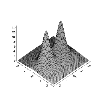
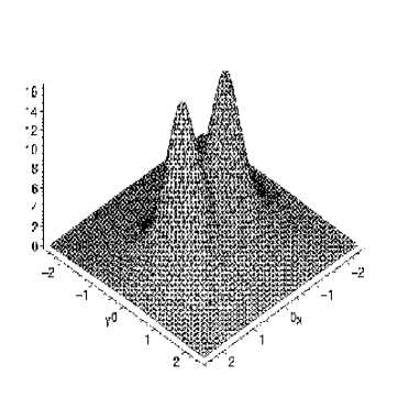
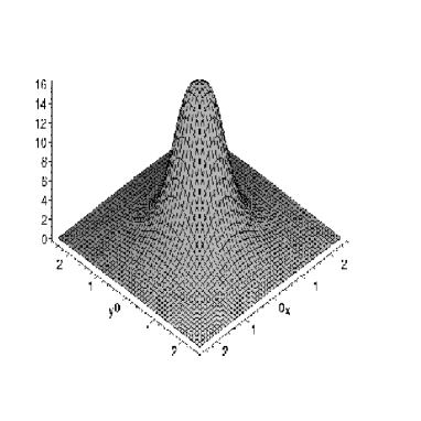
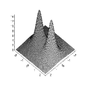
Figure 8: An elastic non-trivial scattering of a soliton-antisoliton configuration in flat spacetime.

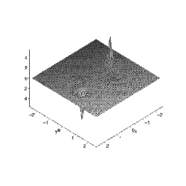
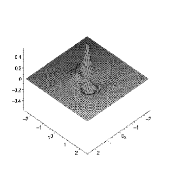
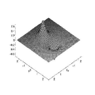
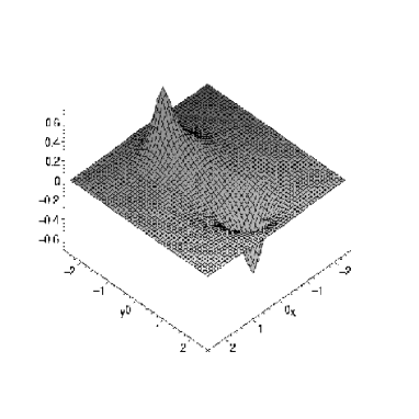
Figure 9: Topological charge density at increasing times for soliton-antisoliton elastic scattering.

• Lets take the simplest case where $f(z)=z$ and $h(\bar{z})=1$. Roughly speaking the chiral field $J$ departs from its asymptotic value $J_{0}$ when $w\rightarrow 0$ which implies that $z\rightarrow\pm\sqrt{-2t}$. More precisely, the two structures, for $t$ negative, are located approximately at $x\approx\pm\sqrt{-2t}$ while, for $t$ positive, they are on the $y$-axis at $y\approx\pm\sqrt{2t}$. Figure 8 illustrates the scattering behavior of our configuration near $t=0$.

  The picture is consistent with the properties of the energy density of the solution which is given by

  $${\cal E}=16\frac{2r^{4}+4r^{2}+4t^{2}(1+2r^{2})-4t(x^{2}-y^{2})+1}{\left(2r^{4}+2r^{2}+4t(x^{2}-y^{2})+4t^{2}+1\right)^{2}}$$ (46)

  and is symmetric under the interchange $t\rightarrow-t,x\rightarrow y,y\rightarrow x$. The time symmetry of the energy density confirms the lack of radiation. However, the corresponding localized structures are not constant of size; in fact, their height is proportional to $t^{-1}$ and their radius is proportional to $\sqrt{t}$.

  The projected topological charge ${\cal N^{\prime}}$ is zero throughout the scattering process while the topological density has an almost identical distribution (up to a scale) to that of the energy density as shown in Figure 9. Therefore, the configuration represents a soliton and an antisoliton that are clearly visible as distinct structures having respectively one and minus one units of topological charge concentrated in a single lump.

In the general case where $h=z^{p}$ and $h=\bar{z}^{q}$, the chiral field $J$ departs from its asymptotic value $J_{0}$ when $w=z^{(p-1)}(2tp+z^{N})\rightarrow 0$ with $N=p+q+1$ which is true when either $z^{(p-1)}=0$ or $2tp+z^{N}=0$ and this is approximately where the lumps are located. So $J$ represent a family of soliton-antisoliton solution which consists of $(p-1)$ static soliton-like objects at the origin with $N$ others accelerating toward them, scattering at an angle of $\pi/N$ and then decelerating as they separate.

Note that in the non-integrable models (usually) there is an attractive force between solitons of opposite topological charge which implies that the initially well separated solitons and antisolitons attract each other and eventually annihilate into a wave of pure radiation which spreads with the velocity of light in a direction perpendicular to the motion of the initial structures as shown in [28]. However, it is known that the interaction forces between solitons and antisolitons do depend on their relative orientation in the internal space which implies that the cross section for the soliton-antisoliton elastic scattering is different than zero. In fact the proton-antiproton elastic scattering is seen in a reasonable fraction of cases. Therefore the analytic construction of families of soliton-antisoliton configurations with elastic scattering properties obtained are of immense importance since not only provide a major link between integrable and non-integrable models but can actually have physical applications in the laboratories.

5 Conclusions

The infinite number of conservation laws associated with a given system place severe constraints upon possible soliton dynamics. The construction of exact analytic multi-solitons with trivial scattering properties is a result of such integrability properties. In this paper soliton and soliton-antisoliton structures have been presented for two planar integrable equations related with the three-spatial dimensional self-dual Yang-Mills-Higgs equations. These structures travel with non-constant velocity, their size is non-constant and they interact non-trivially. As we have already mentioned this non-trivial scattering is not usual in an integrable theory but is exceptional. Such results are useful for investigating the connection between integrable and non-integrable systems which possess multi-soliton solutions. In addition, they indicate the likely occurrence of new phenomena in higher-dimensional soliton theory which are not present in one-dimensional systems.

The multi-pole ansatz have been extended to other planar integrable systems in order to obtain soliton solutions with non-trivial dynamics. In particular, a large class of solutions of the Davey-Stewartson II equation has been constructed in [35] which have an arbitrary rational localization in the plane and describe typical interactions consisting of head-on collisions with a $\pi/2$ scattering angle. Similarly, in [36] the discrete spectrum of the non-stationary Schrodinger equation and localized solutions of the Kadomtsev-Petviashvili I equation are studied via the inverse scattering transform. It was shown that there exist infinitely many real and rationally decaying potentials which correspond to a discrete spectrum whose related eigenfunctions have multiple poles in the spectral parameter; while the resulting localized solutions of the Kadomtsev-Petviashvili I behave as a collection of individual humps with nonuniform dynamics.

It would be interesting to understand the role of higher poles in algebraic-geometry approach like twistor theory (for example, the function $\Psi$ given by (16) correspond to $n=2$ bundles), and also to investigate the construction of the corresponding solutions and their dynamics in de Sitter space. Finally, it would be interesting to extend our construction in higher dimensional gauged theories and investigate the scattering behavior of the corresponding classical solutions and, also, consider and study its noncommutative version (see, for example, Ref. [37]).

References

- [1] M.J. Ablowitz and P.A. Clarkson, Solitons, Nonlinear Evolution Equations and Inverse Scattering, Cambridge University Press (1991)
- [2] W.J. Zakrzewski, Low Dimensional Sigma Models IOP (1989)
- [3] S. Novikov, S.V. Manakov, L.P. Pitaevskii and V.E. Zakhariv, Theory of Solitons, Consults Bureau, NY, (1984)
- [4] B. Konopelchenko and C. Rogers, Phys. Lett. A 158 (1991) 391
- [5] A. Davey and K. Stewartson, Proc. Roy. Soc. Lond. A 360 (1974) 101
- [6] R.S. Ward, J. Math. Phys. 29 (1988) 386
- [7] Y. Matsuno, Int. J. Mod. Phys. B 9 (1995) 1985
- [8] F. Calogero and A. Degasperis, Solitons, Springel-Verlag (1980)
- [9] M. Boiti, J.J.P. Leon, L. Martina and F. Pempinelli, Phys. Lett. 132 (1988) 432
- [10] P.M. Santini, Physica D 41 (1990) 26
- [11] K.A. Gorshkov, D.E. Pelinosky and Y.A. Stepanyants, JETP 77 (1993) 237
- [12] R.S. Ward, Phys. Lett. A 208 (1995) 203
- [13] T. Ioannidou, J. Math. Phys. 37 (1996) 3422
- [14] T. Ioannidou, Nonlinearity 15 (2002) 1498
- [15] M.F. Atiyah, Commun. Math. Phys. 93 (1984) 437
- [16] T. Ioannidou and P.M. Sutcliffe, J. Math. Phys. 40 (1999) 5440
- [17] S. Jarvis and P. Norbury, Bull. London Math. Soc. 29 (1997) 737
- [18] R.S. Ward, Asian J. Math. 3 (1999) 325
- [19] J. Maldacena, Adv. Theor. Math. Phys. 2 (1998) 505
- [20] E. Witten, Adv. Theor. Math. Phys. 2 (1998) 253
- [21] S.W. Hawking and G.F.R. Ellis, The Large-Scale Structure of Space-Time, CUP (1973)
- [22] R.S. Ward, J. Math. Phys. 29 (1988) 386
- [23] Z. Zhou, J. Math. Phys. 42 (2001) 1085
- [24] Z. Zhou, J. Math. Phys. 42 (2001) 4938
- [25] A.S. Fokas and T. Ioannidou, Comm. Appl. Anal. 5 (2001) 235
- [26] A.A. Belavin and V.E. Zakzarov, Phys. Lett. B 73 (1978) 53; V.E. Zakzarov and A.B. Shabat, Funct. Anal. Appl. 13 (1980) 166
- [27] P. Forgacs, Z. Horvath and L. Palla, Nucl. Phys. B 229 (1983) 77
- [28] W. Zakrzewski, Nonlinearity 4 (1991) 429
- [29] K. Uhlenbeck, J. Diff. Geom. 30 (1989) 1
- [30] T. Ioannidou and W.J. Zakrzewski, J. Math. Phys. 39 (1998) 2693
- [31] S. Jarvis, A rational map for Euclidean monopoles via radial scattering, Oxford preprint (1996)
- [32] R.A. Leese, J. Math. Phys. 30 (1989) 2072
- [33] P.M. Sutcliffe, J. Math. Phys. 33 (1992) 2269
- [34] M.J. Borchers and W.D. Garber, Commun. Math. Phys. 72 (1980) 77
- [35] M. Manas and P.M. Santini, Phys. Lett. A 227 (1997) 325
- [36] J. Villarroel and M.J. Ablowitz, Commun. Math. Phys. 207 (1999) 1
- [37] O. Lechtenfeld and A.D. Popov, Phys. Lett. B 523 (2001) 178