New Global Defect Structures
Abstract
We investigate the presence of defects in systems described by real scalar field in (D,1) spacetime dimensions. We show that when the potential assumes specific form, there are models which support stable global defects for D arbitrary. We also show how to find first-order differential equations that solve the equations of motion, and how to solve models in D dimensions via soluble problems in D=1. We illustrate the procedure examining specific models and finding explicit solutions.
pacs:
11.10.Lm, 11.27.+d, 98.80.CqThe search for defect structures of topological nature is of direct interest to high energy physics, in particular to gravity in warped spacetimes involving spatial extra dimensions. Very recently, a great deal of attention has been given to scalar fields coupled to gravity in dimensions rs ; gw ; gt ; grs ; df . Our interest here is related to Ref. campos , which deals with critical behavior of thick branes induced at high temperature, and to Refs. G ; GS ; RS , which study the coupling of scalar and other fields to gravity in warped spacetimes involving two or more extra dimensions.
These specific investigations have motivated us to study defect solutions in models involving scalar field in spacetime dimensions. To do this, however, we have to circumvent a theorem H ; D ; J , which states that models described by a single real scalar field cannot support topological defects, unless we work in space-time dimensions. To evade this problem, in the present letter we consider models described by the Lagrange density where the potential is , and is a real scalar field. The metric is , with in space-time dimensions. has the form , where is a smooth function of , and . We suppose that is a critical point of , such that . This generalization is different from the extensions one usually considers to evade the aforementined problem, which include for instance constraints in the scalar fields and/or the presence of fields with nonzero spin – see, e.g., Ref. vs , and other specific works on the subject ddi ; afz . Potentials of the above form appear for instance in the Gross-Pitaevski equation, which finds applications in several branches of physics – see, e.g., Ref. GP . Other recent examples in dimensions include Ref. SV , which deals with the dynamics of embedded kinks, and Refs. OG , which describe scalar field in distinct backgrounds.
In higher dimensions, the factor that we introduce in Eq. (1) gives rise to an effective model, which comes from a more fundamental theory. To make this point clear, we consider the model which is a simplified Abelian version of the color dielectric model fl in the absence of fermions – see, e.g., Ref. wil . This model describes coupling between the real scalar field and the gauge field , through the dielectric function Here is the gauge field strenght. This model shows that for spherically symmetric static configurations in the electric sector, the equation of motion for the matter field is where is the electric field. The use of the equation of motion for the electric field provides an effective description of the matter field in which the equation of motion exactly reproduces bmm the equation of motion that we will be investigating below, under the choice As one knows, color dielectric models may provide effective descriptions for non-perturbative QCD – see, e.g., Ref. ws for a very recent investigation and for related works.
We now focus attention on the effective model. We investigate the presence of static solutions considering the specific potential
| (1) |
where . We write to obtain the equation of motion The energy density of the field configuration has the form We suppose that solves the equation of motion. It has total energy , which splits into gradient and potential portions. We make the change to get to the conditions
| (2) |
and to make the field configuration stable. Since and , these conditions impose restrictions on both and .
An important case is , and here the value makes , that is, the energy is equally shared between gradient and potential portions. This is the standard result: from H ; D ; J we see that for the special case , there exist stable solutions only in . However, the form of the potential (1) is peculiar, and it allows obtaining several other cases which support defect solutions. In two spatial dimensions, for one gets , but this gives no further relation between the gradient and potential portions of the energy. For we get that to make .
We investigate the possibility of obtaining a Bogomol’nyi bound bog ; ps for the energy of static configurations in the present investigation. The case is standard, so we deal with . We suppose that the static solutions engender spherical symmetry, that is, we consider , with . The energy can be written as , where and is the D-dependent angular factor. This result is obtained if and only if , and the energy is minimized to for static and radial field configurations which solve the first order equations
| (3) |
This is the Bogomol’nyi bound, now generalized to models for scalar field that live in spatial dimensions. The value leads to defect solutions of the BPS type, which obey first order equations and have energy evenly split into gradient and potential portions. For one gets , and in this case the model engenders scale invariance. We can show that solutions of the above first order equations solve the equation of motion (4) for potentials given by Eq. (1). Also, we follow Ref. bms and introduce the ratio . For field configuration that obey and one can show that solutions of the equation of motion also solve the first order equations (3). This extends the result of Ref. bms to the present investigation: it shows that the equation of motion (4) completely factorizes into the two first order equations (3).
The equation of motion for is
| (4) |
The first order equation is given by (3), and their solutions solve the equation of motion and are stable against radial, time-dependent fluctuations. To see this we consider . For small fluctuations we get , where the Hamiltonian can be written as
| (5) |
It is non-negative, and the lowest bound state is the zero mode, which obeys This gives where is the normalization constant, which usually exists only for one of the two sign possibilities. We can also write , which is another way to write the zero mode.
We investigate the presence of defect structures turning attention to specific models in and . We first consider the case We choose . The equation of motion is . We are searching for solutions that obey the boundary conditions and , where is a critical point of the potential, obeying . In this case one can write see bms . In one usually introduces the conserved current . We see that and so gives the energy density of the field configuration bb . Thus, we introduce as the topological charge, which is exactly the total energy of the solution.
We exemplify the case with the family of models
| (6) |
The parameter is real, and it is related to the way the field self-interacts. These models are well-defined for odd, For we get to the standard theory. For we have new models, presenting potentials which support minima at and . For odd the classical bosonic masses at the asymmetric minima are given by . For another minimum appear at . However, the classical mass at this symmetric minimum diverges, signalling that does not define a true perturbative ground state for the system.
We consider odd. The first-order equations are which have solutions We consider the center of the defect at , for simplicity. Their energies are given by , and we plot some of them in Fig. [1].
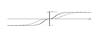
We see that solutions for connect the minima , passing through the symmetric minimum at with vanishing derivative. They are new structures, which solve first-order equations, and we call them 2-kink defects since they seem to be composed of two standard kinks, symmetrically separated by a distance which is proportional to , the parameter that specifies the potential. To see this, we notice that the zero modes are given by where – we use to represent the zero modes. These zero modes concentrate around two symmetric points, which identify each one of the two standard kinks. Defect structures similar to the above 2-kink defects have been studied in the recent past, for instance in Ref. chw , for solutions of the equations of motion in a -symmetric model, and also in Ref. svo , in a supersymmetric theory, for solutions which solve first-order equations. We have studied the model coupled to gravity in warped spacetimes, in dimensions bfg . The results show that it also induces critical behavior similar to Ref. campos , but now the driving parameter is , which indicates the way the scalar field self-interacts, and not the temperature anymore.
The cases with even are different. The case is special: it gives the potential , which supports the nontopological or lumplike solution The lumplike solution is unstable, as we can see from the zero mode, which is proportional to : the zero mode has a node, so there must be a lower (negative energy) eigenvalue. In the present case, the tachyonic eigenvalue can be calculated exactly since the quantum-mechanical potential associated with stability of the lumplike configuration has the form . This potential supports three bound states, the first being a tachyonic eigenfunction with eigenvalue , the second the zero mode, and the third a positive energy bound state with . As one knows, tachyons appear in String Theory W ; KS and this has brought renewed interest on the subject – see, e.g., Refs. S ; Z ; MZ .
The other cases for even are These cases require that in Eq. (6), but we can also change in Eq. (6) and consider . We investigate the case ; reflection symmetry leads to the other case. We notice that the origin is also a minimum, with null derivative. These models also support topological defects, in the form , with energies for These solutions solve the first order equation ; the other equation is solved by .
We now consider , and . The equation of motion is . We search for solution , which only depends on the radial coordinate, obeying and . In this case we get
| (7) |
We write to get This result maps the model into the model.
We see that which shows that the full line is mapped to . We notice that since the center of the defect is arbitrary, so is the point in ; thus the solution introduces no fundamental scale, in accordance with the scale symmetry that the model engenders. If one uses the model (6) with odd to define the potential in this case, we get the solutions
| (8) |
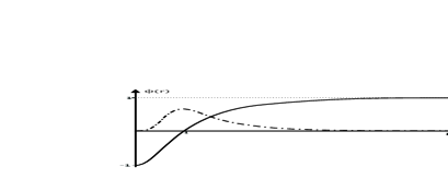
Their energies are . In Fig. [2] we depict the defect solution for . The corresponding zero mode is given by This zero mode binds around the circle where the defect solution vanishes, as we show in Fig. [2], where we also plot .
The last case is , with . The equation of motion for is
| (9) |
We write to get and again, we map the model into a one-dimensional problem. We solve to get . This shows that is now in or , and so we have to use the upper sign for , or the lower sign for . We can use the model of Eq. (6) for to solve the D-dimensional problem with . In this case the solutions are
| (10) |
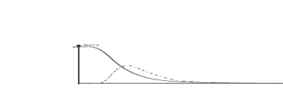
for Their energies are given by , and in Fig. [3] we depict the solution for .
In the case of and the zero mode is given by we could not find the normalization factor explicitly in this case. We plot in Fig. [3] to show that the zero mode binds at the skin of the defect solution, concentrating around the radius of the defect, which is given by .
The solutions that we have found have a central core, and a skin which depends on the parameters that specify the potential of the model. They are stable, well distinct of other known defects such as the bubbles formed from unstable domain walls – see for instance Refs. b1 ; b2 ; b3 ; b4 . Also, they are neutral structures, and may contribute to curve spacetime, and to affect cosmic evolution. They may become charged if charged bosons and/or fermions bind to them. For instance, if one couples Dirac fermions with the Yukawa coupling , the fermionic zero modes are similar to the bosonic zero modes that we have just presented. In Ref. bmm we investigate these and other issues in detail.
We end this letter recalling that we have solved the equation of motion using . Although this identification works very naturally for the first order equations, we used the equation of motion to present a more general investigation, which may be extended to tachyons in spatial dimensions. For instance, from the lumplike solution for and we can obtain another lumplike solution which is valid for . Another issue concerns the identification of the topological behavior of the above defect structures. We do this introducing the (generalized current-like) tensor It obeys for which means that the quantities constitute a family of distinct conserved (generalized charge) densities. We introduce the scalar quantity which generalizes the standard result, obtained with – see the reasoning above Eq. (6). Thus, we define the topological charge as , which exposes the topological behavior of the new global defect structures that we have just found.
We would like to thank R. Jackiw for drawing our attention to Ref. H . We also thank CAPES, CNPq, PROCAD and PRONEX for partial support.
References
- (1) L. Randall and R. Sundrum, Phys. Rev. Lett. 83, 3370 (1999) and 83, 4690 (1999).
- (2) W.D. Goldberger and M.B. Wise, Phys. Rev. Lett. 83, 4922 (1999).
- (3) J. Garriga and T. Tanaka, Phys. Rev. Lett. 84, 2778 (2000).
- (4) R. Gregory, V.A. Rubakov, and S.M. Sibiryakov, Phys. Rev. Lett. 84, 5928 (2000).
- (5) O. DeWolfe, D.Z. Freedman, S.S. Gubser, and A. Karch, Phys. Rev. D 62, 046008 (2000).
- (6) A. Campos, Phys. Rev. Lett. 88, 141602 (2002).
- (7) R. Gregory, Phys. Rev. Lett. 84, 2564 (2000).
- (8) T. Gherghetta and M. Shaposhnikov, Phys. Rev. Lett. 85, 240 (2000).
- (9) E. Roessl and M. Shaposhnikov, Phys. Rev. D 66, 084008 (2002).
- (10) R. Hobart, Proc. Phys. Soc. Lond. 82, 201 (1963).
- (11) G.H. Derrick, J. Math. Phys. 5, 1252 (1964).
- (12) R. Jackiw, Rev. Mod. Phys. 49, 681 (1977).
- (13) A. Vilenkin and E.P.S. Shellard, Cosmic Strings and other Topological Defects (Cambridge UP, Cambridge/UK, 1994).
- (14) S. Deser, M.J. Duff, and C.J. Isham, Nucl. Phys. B 114, 29 (1976).
- (15) H. Aratyn, L.A. Ferreira, and A.H. Zimerman, Phys. Rev. Lett. 83, 1723 (1999).
- (16) F. Dalfovo, S. Giorgini, L.P. Pitaevski, and S. Stringari, Rev. Mod. Phys. 71, 463 (1999).
- (17) M. Salem and T. Vachaspati, Phys. Rev. D 66, 025003 (2002).
- (18) K.D. Olum and N. Graham, Phys. Lett. B 554, 175 (2003); N. Graham and K.D. Olum, Phys. Rev. D 67, 085014 (2003).
- (19) R. Friedberg and T.D. Lee, Phys. Rev. D 15, 1694 (1977); 16, 1096 (1977); 18, 2623 (1978).
- (20) L. Wilets, Nontopological Solitons (World Scientific, Singapore, 1989).
- (21) D. Bazeia, J. Menezes, and R. Menezes, work in progress.
- (22) A. Wereszczyński and M. Ślusarczyk, Eur. Phys. J C, in print, hep-ph/0307213.
- (23) E.B. Bogomol’nyi, Sov. J. Nucl. Phys. 24, 449 (1976).
- (24) M.K. Prasad and C.M. Sommerfield, Phys. Rev. Lett. 35, 760 (1975).
- (25) D. Bazeia, J. Menezes, and M.M. Santos, Phys. Lett. B 521, 418 (2001); Nucl. Phys. B 636, 132 (2002).
- (26) D. Bazeia and F.A. Brito, Phys. Rev. Lett. 84, 1094 (2000).
- (27) A. Campos, K. Holland, and U.-J. Wiese, Phys. Rev. Lett. 81, 2420 (1998).
- (28) M.A. Shifman and M.B. Voloshin, Phys. Rev. D 57, 2590 (1998).
- (29) D. Bazeia, C. Furtado, and A.R. Gomes, hep-th/0308084.
- (30) E. Witten. Nucl. Phys. B 268, 253 (1986).
- (31) V.A. Kostelecký and S. Samuel, Phys. Lett. B. 207, 169 (1988); Nucl. Phys. 336, 263 (1990).
- (32) A. Sen, Int. J. Mod. Phys. A 14, 4061 (1999); J. High Energy Phys. 12, 027 (1999).
- (33) B. Zwiebach, J. High Energy Phys. 09 028 (2000).
- (34) J.A. Minahan and B. Zwiebach, J. High Energy Phys. 09, 029 (2000).
- (35) J.A. Frieman, G.B. Gelmini, M. Gleiser, and E.W. Kolb, Phys. Rev. Lett. 60, 2101 (1988).
- (36) A.L. MacPherson and B.A. Campbell, Phys. Lett. B 347, 205 (1995).
- (37) D. Coulson, Z. Lalak, and B. Ovrut, Phys. Rev. D 53, 4237 (1996).
- (38) J.R. Morris and D. Bazeia, Phys. Rev. D 54, 5217 (1996).