OCU-200

AP-GR-10

Compact Einstein Spaces based on Quaternionic Kähler Manifolds
Mitsuo Hiragane, Yukinori Yasui and Hideki Ishihara Department of Physics, Osaka City University
Sumiyoshi-ku, Osaka, 558-8585, Japan

We investigate the Einstein equation with a positive cosmological constant for $4n+4$-dimensional metrics on bundles over Quaternionic Kähler base manifolds whose fibers are 4-dimensional Bianchi IX manifolds. The Einstein equations are reduced to a set of non-linear ordinary differential equations. We numerically find inhomogeneous compact Einstein spaces with orbifold singularity.

1 Introduction

Compact Einstein spaces with positive-definite metrics have been studied extensively: first, the spaces are considered as candidates of compact internal spaces which are admitted in higher-dimensional gravitational theories[1]; and secondly, the spaces are expected that they may dominate the path integrals of quantum gravity[2].

There are many examples of homogeneous Einstein metrics to be found in a lot of literature, but they are very exceptional among general Einstein spaces. In contrast, the inhomogeneous Einstein metrics would cover wide range, but our knowledge for them seems to be largely limited. The first example of inhomogeneous compact Einstein space which is a solution to the Einstein equation with a positive cosmological constant,

$$\hat{R}_{ab}=\Lambda\hat{g}_{ab},$$ (1.1)

was constructed by Page[3] by taking a limit of the Euclidean Kerr-de Sitter solution, and it was generalized by Bérard-Bergery[4].

In the absence of any general understanding of the solution to the Einstein equation (1.1), one of the standard strategies for constructing inhomogeneous examples is to study the space with cohomogeneity one metric: the space admits a Lie group action by isometries whose orbits span the space with codimension one. It is considered that the space which foliates into a sequence of homogeneous subspaces of codimension one. The Einstein equation for such metric reduces to a set of non-linear second order ordinary differential equations[5].

It is possible to replace the homogeneous subspaces by spaces with bundle structure. This idea originates from the Kaluza-Klein construction. The Einstein equation translates into a coupled system of equations involving the Ricci curvatures of the fibers and base space, as well as the curvature of the connection. When we have a suitable choice for the bundle space and connection, the Einstein equation also reduces to a set of the ordinary differential equations.

In this paper, we construct compact inhomogeneous examples of the Einstein metric with a positive cosmological constant in 4n+4 dimensions on the spaces with bundle structure. More precisely we consider the union of principal $SO(3)$-bundles $P$ over Quaternionic Kähler manifolds, so our spaces may be identified locally with $I\times P$ for some interval $I$ of the real line. This geometrical setting was studied in [6] and they constructed a family of inhomogeneous compact Einstein spaces. Our construction is a generalization of their system[6, 7, 8].

In this framework, it is possible to take three types of boundary conditions at two endpoints of $I$ for completeness, i.e., two types of bolt singularities associated with the Quaternionic Kähler manifold and with its twistor space respectively, and the nut singularity describing $S^{4n+3}$-collapsing. We find new compact Einstein spaces which have the two types of bolts, numerically. The new solutions together with the known solutions give a unified description of compact Einstein spaces with a positive cosmological constant.

The paper is organized as follows: Section 2 contains our Kaluza-Klein metric ansatz and calculations of the Riemannian curvature. In section 3 we derive the Einstein equation after a short review of Quaternionic Kähler manifolds. We also prove the diagonalizability of the metric using the technique for the 4-dimensional Bianchi IX metric. In section 4, we discuss the boundary conditions and give asymptotic solutions near the boundaries. In section 5, known exact solutions are listed. In section 6 we present new solutions obtained by numerical integrations. Section 7 is devoted to summary and discussion.

2 Metric Ansatz and Curvature Calculation

In this section, we shall consider metrics on ($m+4$)-dimensional manifolds $\widehat{M}$. To make the analysis manageable, we assume the following geometrical condition for $\widehat{M}$. Let $\pi:P\longrightarrow M$ be a principal $SO(3)$-bundle over an $m$-dimensional Riemannian manifold ($M,g_{M}$) and $\phi$ be an $SO(3)$-connection on $P$. The connection $\phi$ locally takes the form

$$\phi=s^{-1}As+s^{-1}ds,\quad s\in SO(3).$$ (2.1)

Here, $A$ is an $so(3)$-valued local 1-form on $M$ and $s^{-1}ds$ is considered as the Maurer-Cartan form. Let $\phi^{i}$ be the components of $\phi$ for the standard basis {$E_{i}$} of $so(3)$ which satisfies the Lie bracket relations $[E_{i},E_{j}]=\sum_{k=1}^{3}\varepsilon_{ijk}E_{k}$. By using the left-invariant 1-forms $\sigma^{i}$ defined by $s^{-1}ds=\sum_{i=1}^{3}\sigma^{i}E_{i}$, the equation (2.1) can be also written as

$$\phi^{i}=\sum_{j=1}^{3}A^{j}{\mathcal{O}}_{ji}+\sigma^{i}$$ (2.2)

with the adjoint representation

$$s^{-1}E_{i}s=\sum_{j=1}^{3}{\mathcal{O}}_{ij}E_{j}~{}.$$ (2.3)

In this setting we consider metrics on $\widehat{M}$ which is locally the product space $I\times P$, where $I$ denotes some interval of R. Given a metric $b_{ij}$ on $SO(3)$, the Kaluza-Klein metric takes the form

$$\hat{g}=dt^{2}+\sum_{i,j=1}^{3}b_{ij}(t)\phi^{i}\phi^{j}+f(t)^{2}g_{M}\,.$$ (2.4)

We can show that the matrix $b_{ij}(t)$ is diagonalizable for all $t$ under a certain condition of the base space $M$  (see a proposition in section 3). Thus we write the metric as

$$\hat{g}=dt^{2}+a(t)^{2}(\phi^{1})^{2}+b(t)^{2}(\phi^{2})^{2}+c(t)^{2}(\phi^{3})^{2}+f(t)^{2}g_{M}.$$ (2.5)

If we impose the condition $a=b=c$, then the metric (2.5) has an isometry $SO(3)$. Otherwise it has no such symmetry because of the explicit dependence on the group element ${\mathcal{O}}_{ij}$.

Now, we choose an orthonormal basis $\hat{e}^{a}=\{\hat{e}^{0},\;\hat{e}^{i},\;\hat{e}^{\alpha}\;;\;i=1\sim 3,\;\alpha=1\sim m\}$ for (2.5),

$$\hat{e}^{0}=dt,\quad\hat{e}^{i}=a_{i}\phi^{i},\quad\hat{e}^{\alpha}=fe^{\alpha}~{},$$ (2.6)

where $(a_{i})=(a,~{}b,~{}c)$ and $e^{\alpha}$ is an orthonormal basis for $g_{M}$. Then, the spin connection $\hat{\omega}_{ab}$ defined by $d\hat{e}^{a}=-\hat{\omega}_{ab}\wedge\hat{e}^{b}$ is calculated as

$$\begin{array}[]{c}\hat{\omega}_{0i}=-\cfrac{\dot{a}_{i}}{a_{i}}\,\hat{e}^{i}\,,\quad\hat{\omega}_{0\alpha}=-\cfrac{\dot{f}}{f}\,\hat{e}^{\alpha}\,,\quad\hat{\omega}_{ij}=\cfrac{1}{2}\,{\displaystyle\sum_{k}}\varepsilon_{ijk}\cfrac{a_{k}^{2}-a_{i}^{2}-a_{j}^{2}}{a_{i}a_{j}a_{k}}\,\hat{e}^{k},\\[15.0pt] \hat{\omega}_{i\alpha}=\cfrac{a_{i}}{2f^{2}}~{}{\displaystyle\sum_{k,\beta}}{\mathcal{O}}_{ki}F^{k}_{\alpha\beta}\hat{e}^{\beta}\,,\quad\hat{\omega}_{\alpha\beta}=\omega_{\alpha\beta}-{\displaystyle\sum_{k,i}}\cfrac{a_{i}}{2f^{2}}~{}{\mathcal{O}}_{ki}F^{k}_{\alpha\beta}\hat{e}^{i}\,,\end{array}$$ (2.7)

where $F=\sum_{i}F^{i}E_{i}$ is the curvature 2-form of $A$ and $\omega_{\alpha\beta}$ is the spin connection on $M$. The curvature 2-form $\widehat{\Omega}_{ab}=d\hat{\omega}_{ab}+\sum_{c}\hat{\omega}_{ac}\wedge\hat{\omega}_{cb}$ is given by the following equations:

$$\widehat{\Omega}_{0i} = -\cfrac{\ddot{a}_{i}}{a_{i}}\hat{e}^{0}\wedge\hat{e}^{i}+\cfrac{1}{2}\,\displaystyle{\sum_{j,k}}\varepsilon_{ijk}\left[\cfrac{\dot{a}_{i}}{a_{j}a_{k}}+\cfrac{\dot{a}_{j}}{a_{j}}\,\cfrac{a_{k}^{2}-a_{i}^{2}-a_{j}^{2}}{a_{i}a_{j}a_{k}}\,\right]\hat{e}^{j}\wedge\hat{e}^{k}$$

$$-\cfrac{a_{i}}{2f^{2}}\left(\cfrac{\dot{a}_{i}}{a_{i}}-\cfrac{\dot{f}}{f}\right)\displaystyle{\sum_{k,\alpha,\beta}}{\mathcal{O}}_{ki}F^{k}_{\alpha\beta}\hat{e}^{\alpha}\wedge\hat{e}^{\beta},$$

$$\widehat{\Omega}_{0\alpha} = -\cfrac{\ddot{f}}{f}\hat{e}^{0}\wedge\hat{e}^{\alpha}-\cfrac{a_{i}}{2f^{2}}\left(\cfrac{\dot{a}_{i}}{a_{i}}-\cfrac{\dot{f}}{f}\right)\displaystyle{\sum_{k,i,\beta}}{\mathcal{O}}_{ki}F^{k}_{\alpha\beta}\hat{e}^{i}\wedge\hat{e}^{\beta},$$

$$\widehat{\Omega}_{i\alpha} = -\displaystyle{\sum_{j,\beta}}\left[\cfrac{\dot{a_{i}}\dot{f}}{a_{i}f}~{}\delta_{ij}\delta_{\alpha\beta}+\displaystyle{\sum_{k,l}}\cfrac{1}{4f^{2}}\varepsilon_{ijl}\cfrac{a^{2}_{i}+a^{2}_{j}-a^{2}_{l}}{a_{i}a_{j}}~{}{\mathcal{O}}_{kl}F^{k}_{\alpha\beta}-\displaystyle{\sum_{k,l,\gamma}}\cfrac{1}{4f^{4}}a_{i}a_{j}{\mathcal{O}}_{ki}F^{k}_{\beta\gamma}{\mathcal{O}}_{lj}F^{l}_{\alpha\gamma}\right]\hat{e}^{j}\wedge\hat{e}^{\beta}$$

$$+\cfrac{1}{2}\left(\cfrac{\dot{a_{i}}}{f^{2}}-a_{i}\cfrac{\dot{f}}{f}\right)\displaystyle{\sum_{k,\beta}}{\mathcal{O}}_{ki}F^{k}_{\alpha\beta}\hat{e}^{0}\wedge\hat{e}^{\beta}-\cfrac{a_{i}}{2f^{3}}\displaystyle{\sum_{k,\beta,\gamma}}{\mathcal{O}}_{ki}\left(D_{\gamma}F^{k}_{\alpha\beta}\right)\hat{e}^{\beta}\wedge\hat{e}^{\gamma}\,,$$

$$\widehat{\Omega}_{\alpha\beta} = \Omega_{\alpha\beta}-\cfrac{{\dot{f}}^{2}}{f^{2}}\hat{e}^{\alpha}\wedge\hat{e}^{\beta}-\displaystyle{\sum_{i,k,l}\sum_{\gamma,\delta}}\cfrac{a_{i}^{2}}{4f^{4}}\left({\mathcal{O}}_{ki}F^{k}_{\alpha\beta}{\mathcal{O}}_{li}F^{l}_{\gamma\delta}+{\mathcal{O}}_{ki}F^{k}_{\alpha\gamma}{\mathcal{O}}_{li}F^{l}_{\beta\delta}\right)\hat{e}^{\gamma}\wedge\hat{e}^{\delta}$$

$$+\displaystyle{\sum_{i,k}}\displaystyle{\sum_{\gamma}}\cfrac{a_{i}}{2f^{3}}{\mathcal{O}}_{ki}\left(D_{\gamma}F^{k}_{\alpha\beta}\right)\hat{e}^{i}\wedge\hat{e}^{\gamma}-\displaystyle{\sum_{i,k}}\left(\cfrac{\dot{a_{i}}}{f^{2}}-a_{i}\cfrac{\dot{f}}{f^{3}}\right){\mathcal{O}}_{ki}F^{k}_{\alpha\beta}\hat{e}^{0}\wedge\hat{e}^{i}$$

$$+\displaystyle{\sum_{i,j}}\displaystyle{\sum_{k,l}}\displaystyle{\sum_{\gamma}}\cfrac{a_{i}a_{j}}{4f^{4}}{\mathcal{O}}_{ki}F^{k}_{\alpha\gamma}{\mathcal{O}}_{lj}F^{l}_{\gamma\beta}\hat{e}^{i}\wedge\hat{e}^{j}$$

$$-\cfrac{1}{2f^{2}}\displaystyle{\sum_{k}}F^{k}_{\alpha\beta}\left[{\mathcal{O}}_{k1}\cfrac{a^{2}_{2}+a^{2}_{3}-a^{2}_{1}}{a_{2}a_{3}}\;\hat{e}^{2}\wedge\hat{e}^{3}+{\mathcal{O}}_{k2}\cfrac{a^{2}_{3}+a^{2}_{1}-a^{2}_{2}}{a_{3}a_{1}}\hat{e}^{3}\wedge\hat{e}^{1}\right.$$

$$\qquad\left.+{\mathcal{O}}_{k3}\cfrac{a^{2}_{1}+a^{2}_{2}-a^{2}_{3}}{a_{1}a_{2}}\hat{e}^{1}\wedge\hat{e}^{2}\right]\,,$$

where $\Omega_{\alpha\beta}$ is the curvature on $M$ and $D_{\gamma}F^{k}_{\alpha\beta}$ is the gauge covariant derivative of $F$,

$$D_{\gamma}F^{k}_{\alpha\beta}=\nabla_{\gamma}F^{k}_{\alpha\beta}+\sum_{i,j}\varepsilon_{kij}A^{i}F^{j}_{\alpha\beta}~{}.$$ (2.8)

The remaining components $\widehat{\Omega}_{ij}$ ($i,j=1\sim 3$) are

$$\widehat{\Omega}_{12}= \left[\cfrac{\dot{a}_{3}}{a_{1}a_{2}}-\cfrac{\dot{a}_{1}}{a_{1}}\;\cfrac{a^{2}_{3}+a^{2}_{1}-a^{2}_{2}}{2a_{1}a_{2}a_{3}}-\cfrac{\dot{a}_{2}}{a_{2}}\;\cfrac{a^{2}_{3}-a^{2}_{1}+a^{2}_{2}}{2a_{1}a_{2}a_{3}}\right]\hat{e}^{0}\wedge\hat{e}^{3}$$ (2.9)

$$-\left[\cfrac{\dot{a}_{1}\dot{a}_{2}}{a_{1}a_{2}}+\cfrac{a^{2}_{3}-a^{2}_{1}-a^{2}_{2}}{2a^{2}_{1}a^{2}_{2}}+\cfrac{a^{4}_{3}-(a^{2}_{1}-a^{2}_{2})^{2}}{4a^{2}_{1}a^{2}_{2}a^{2}_{3}}\right]\hat{e}^{1}\wedge\hat{e}^{2}$$

$$+\cfrac{1}{4f^{2}}{\sum_{k}}\sum_{\alpha,\beta}\left[\cfrac{a^{2}_{3}-a^{2}_{1}-a^{2}_{2}}{a_{1}a_{2}}~{}{\mathcal{O}}_{k3}F^{k}_{\alpha\beta}-\cfrac{a_{1}a_{2}}{f^{2}}~{}{\sum_{l,\gamma}}{\mathcal{O}}_{k1}F^{k}_{\alpha\gamma}{\mathcal{O}}_{l2}F^{l}_{\beta\gamma}\right]\hat{e}_{\alpha}\wedge\hat{e}_{\beta}~{},$$

and $\widehat{\Omega}_{23},\;\widehat{\Omega}_{31}$ are given by cyclic permutations $1\rightarrow 2\rightarrow 3\rightarrow 1$. The non-zero components of Ricci tensor $\widehat{R}_{ab}$ become

$$\widehat{R}_{00} =-{\sum_{i}}\frac{\ddot{a_{i}}}{a_{i}}-m\frac{\ddot{f}}{f}~{},$$ (2.10)

$$\widehat{R}_{ij} =\left[-\frac{d}{dt}\left(\frac{\dot{a_{i}}}{a_{i}}\right)-\frac{\dot{a_{i}}}{a_{i}}\left(\sum_{k}\frac{\dot{a_{k}}}{a_{k}}+m\frac{\dot{f}}{f}\right)\right]\delta_{ij}+R^{SO(3)}_{ij}+\frac{a_{i}a_{j}}{4f^{4}}~{}\sum_{k,l}\sum_{\alpha,\gamma}{\mathcal{O}}_{ki}F^{k}_{\alpha\gamma}{\mathcal{O}}_{lj}F^{l}_{\alpha\gamma}~{},$$

$$\widehat{R}_{\alpha\beta} =\left(-\frac{\ddot{f}}{f}-(m-1)\frac{\dot{f}^{2}}{f^{2}}-\sum_{i}\frac{\dot{a}_{i}\dot{f}}{a_{i}f}\right)\delta_{\alpha\beta}+\cfrac{1}{f^{2}}~{}R_{\alpha\beta}-\sum_{i,k,l}\sum_{\gamma}\frac{a^{2}_{i}}{2f^{4}}~{}{\mathcal{O}}_{ki}F^{k}_{\alpha\gamma}{\mathcal{O}}_{li}F^{l}_{\beta\gamma}~{},$$

$$\widehat{R}_{i\alpha} =\frac{a_{i}}{2f^{3}}~{}\sum_{k,\beta}{\mathcal{O}}_{ki}D_{\beta}F^{k}_{\alpha\beta}.$$

Here $R_{\alpha\beta}$ denotes the Ricci tensor on $M$ and $R^{SO(3)}_{ij}$ the Ricci tensor on $SO(3)$. Explicitly the non-zero components of $R^{SO(3)}_{ij}$ are given by

$$R^{SO(3)}_{11}=\cfrac{a^{4}_{1}-(a^{2}_{2}-a^{2}_{3})^{2}}{2a^{2}_{1}a^{2}_{2}a^{2}_{3}}\,,\;R^{SO(3)}_{22}=\cfrac{a^{4}_{2}-(a^{2}_{3}-a^{2}_{1})^{2}}{2a^{2}_{1}a^{2}_{2}a^{2}_{3}}\,,\;R^{SO(3)}_{33}=\cfrac{a^{4}_{3}-(a^{2}_{1}-a^{2}_{2})^{2}}{2a^{2}_{1}a^{2}_{2}a^{2}_{3}}\,.$$ (2.11)

3 Einstein equation based on Quaternionic Kähler Manifold

In order to solve the Einstein equation, we need a further assumption on the base space $M$ of the principal bundle $P$. Then we will obtain a generalization of the ordinary differential equations studied in [6, 7, 8].

Let ($M,g_{M}$) be a 4n-dimensional Quaternionic Kähler manifold (QK manifold). It has a set of three almost complex structures $J^{a}(a=1\sim 3)$ which satisfy the quaternion algebra

$$J^{a}J^{b}=-\delta_{ab}+\varepsilon_{abc}J^{c}\,,$$ (3.1)

and one can find local 1-forms $A^{i}$ such that

$$\nabla J^{a}=\varepsilon_{abc}A^{b}\otimes J^{c}\,,$$ (3.2)

where $\nabla$ denotes the Levi-Civita connection[9]. According to [10], we introduce an orthonormal basis with 2-indices {$e^{\mu i}$};

$$g_{M}=\sum_{\mu=0}^{3}\sum_{i=1}^{n}e^{\mu i}\otimes e^{\mu i}~{}.$$ (3.3)

Then the 2-forms $J^{a}$ are given by

$$J^{1}=\sum_{i=1}^{3}e^{0i}\wedge e^{1i}+e^{2i}\wedge e^{3i}~{},$$ (3.4)

$$J^{2}=\sum_{i=1}^{3}e^{0i}\wedge e^{2i}+e^{3i}\wedge e^{1i}~{},$$

$$J^{3}=\sum_{i=1}^{3}e^{0i}\wedge e^{3i}+e^{1i}\wedge e^{2i}~{}.$$

Furthermore, the $SO(3)$-connection $A=\sum_{i=1}^{3}A^{i}E_{i}$ is $c_{1}$-self-dual in the sense of [10], i.e., the Yang-Mills curvature $F=dA+A\wedge A$ satisfies the following self-dual equation

$$\ast F=c_{1}\;F\wedge\Omega^{n-1},\quad\Omega=\sum_{a=1}^{3}J^{a}\wedge J^{a}$$ (3.5)

with $c_{1}=6n/(2n+1)!$ . We note that the connection $A$ automatically satisfies the Yang-Mills equation like a 4-dimenional ordinary instanton. In fact

$$D\ast F=c_{1}D(F\wedge\Omega^{n-1})=0~{},$$ (3.6)

where we have used $d\Omega=0$ by (3.2) and the Bianchi identity $DF=0$. It is known that any QK manifold is Einstein and $F$ simply takes the form[9][11]

$$F^{a}=\cfrac{\lambda}{n+2}\;J^{a}~{},$$ (3.7)

where $\lambda$ is the Einstein constant for the metric $g_{M}$.

Now let us turn to the evaluation of the Ricci tensor (2.10). From QK geometry, we saw that the $SO(3)$-connection $A$ is $c_{1}$-self-dual and its curvature satisfies the quaternionic relations. Thus, when we take a 4n-dimensional QK manifold as the base space with self-dual connection, we have

$$R_{\alpha\beta}=(n+2)~{}\delta_{\alpha\beta}~{},\quad\sum_{\alpha}D_{\alpha}F^{i}_{\alpha\beta}=0$$ (3.8)

and

$$\sum_{\alpha,\beta}F^{i}_{\alpha\beta}F^{i}_{\alpha\beta}=4n\delta_{ij}~{},$$ (3.9)

$$\sum_{k,l}\sum_{\gamma}{\mathcal{O}}_{ki}F^{k}_{\alpha\gamma}{\mathcal{O}}_{li}F^{l}_{\beta\gamma}=\sum_{k,l}{\mathcal{O}}_{ki}{\mathcal{O}}_{li}~{}(\delta^{kl}\delta_{\alpha\beta}+\varepsilon_{klj}F^{j}_{\alpha\beta})=\delta_{ii}~{}\delta_{\alpha\beta}~{}.$$

These equations finally lead us to the (4n+4)-dimensional Einstein equation with a cosmological constant $\Lambda$:

$$\cfrac{\ddot{a}}{a} +\cfrac{\ddot{b}}{b}+\cfrac{\ddot{c}}{c}+4n\cfrac{\ddot{f}}{f}=-\Lambda~{}.$$ (3.10)

$$\cfrac{\ddot{a}}{a} =-\cfrac{\dot{a}}{a}\left(\cfrac{\dot{b}}{b}+\cfrac{\dot{c}}{c}+4n\cfrac{\dot{f}}{f}\right)+\cfrac{a^{4}-(b^{2}-c^{2})^{2}}{2a^{2}b^{2}c^{2}}+n\cfrac{a^{2}}{f^{4}}-\Lambda~{},$$

$$\cfrac{\ddot{b}}{b} =-\cfrac{\dot{b}}{b}\left(\cfrac{\dot{c}}{c}+\cfrac{\dot{a}}{a}+4n\cfrac{\dot{f}}{f}\right)+\cfrac{b^{4}-(c^{2}-a^{2})^{2}}{2a^{2}b^{2}c^{2}}+n\cfrac{b^{2}}{f^{4}}-\Lambda~{},$$

$$\cfrac{\ddot{c}}{c} =-\cfrac{\dot{c}}{c}\left(\cfrac{\dot{a}}{a}+\cfrac{\dot{b}}{b}+4n\cfrac{\dot{f}}{f}\right)+\cfrac{c^{4}-(a^{2}-b^{2})^{2}}{2a^{2}b^{2}c^{2}}+n\cfrac{c^{2}}{f^{4}}-\Lambda~{},$$

$$\cfrac{\ddot{f}}{f} =-\cfrac{\dot{f}}{f}\left(\cfrac{\dot{a}}{a}+\cfrac{\dot{b}}{b}+\cfrac{\dot{c}}{c}+(4n-1)\cfrac{\dot{f}}{f}\right)-\cfrac{a^{2}+b^{2}+c^{2}}{2f^{4}}+\cfrac{n+2}{f^{2}}-\Lambda~{}.$$

Here, if we impose the conditions $a=b=c\neq f$ and $a\neq b=c=f~{}$, then (3.10) yields the equation studied in [6] and [7], respectively (see section 5). Also the singular reduction $a\equiv 0~{}$ and $b=c$ gives the $(4n+3)$-dimensional Einstein equation discussed in [8]. In case of the trivial bundle $P=M\times SO(3)$, i.e., $A=0$, the Ricci tensor (2.10) directly yields the Einstein equation without the assumption of QK manifolds. This equation is simply given by dropping the $f^{-4}$ terms and replacing the dimension $4n$ by arbitrary one in (3.10).

It is worth noting that the $8$-dimensional Einstein equation with vanishing $\Lambda$ is special in the sense that the $Spin(7)$ holonomy condition leads to the following first-order equations[12, 13];

$$\cfrac{\dot{a}}{a} =\cfrac{a^{2}-(b-c)^{2}}{2abc}-\cfrac{a}{f^{2}},$$ (3.11)

$$\cfrac{\dot{b}}{b} =\cfrac{b^{2}-(c-a)^{2}}{2abc}-\cfrac{b}{f^{2}},$$

$$\cfrac{\dot{c}}{c} =\cfrac{c^{2}-(a-b)^{2}}{2abc}-\cfrac{c}{f^{2}},$$

$$\cfrac{\dot{f}}{f} =\cfrac{a+b+c}{2f^{2}}.$$

We can verify by substituting (3.11) into (3.10) with $n=1$ that the metric is indeed Ricci-flat, and the explicit solutions were constructed in [8, 13, 14, 15].

Finally we prove the following as mentioned in section 2 :

Proposition  Let $(M,~{}g_{M})$ be a 4n-dimensional QK manifold with $c_{1}$-self-dual connection. Then the Kaluza-Klein metric (2.4) for the Einstein space can be put in the diagonal form (2.5) for all $t$.

Proof.  We calculate the Ricci tensor for the metric (2.4), and the result is given in Appendix A. Note that the off-diagonal component $R_{0i}$ takes the same form as the 4-dimensional Bianchi IX type cosmological model. So this enables us in the usual way (see [16], for example) to diagonalize the metric for all $t$ . The argument is based on an important property of the Einstein equation, namely invariance under the right action of $SO(3)$. Indeed, using the corresponding transformation of the connection

$$\phi\longrightarrow\tilde{\phi}=s_{0}^{-1}\phi~{}s_{0}~{},\quad s_{0}\in SO(3)~{},$$ (3.12)

we can diagonalize the fiber metric $b_{ij}$ at an initial time $t=t_{0}$. Then the Einstein equation $R_{0i}=0$ leads to $\dot{b}_{ij}=0$ for $i\neq j$ at $t=t_{0}$, which implies the diagonality of the solution for all time.

4 Boundary Condition

In this section, we discuss boundary conditions for the Einstein equation (3.10). Let us assume the following compact conditions of $\widehat{M}\simeq I\times P$ :

1. $I$ is the closed interval $[t_{1},t_{2}]$ ,

2. QK manifolds have a positive scalar curvature, namely $\lambda>0$.

Furthermore we require that the singularities at the boundaries $t_{1}$ and $t_{2}$ are resolved by bolts or nuts; there are three types of resolutions, nut $\leftrightarrow$ nut,  bolt $\leftrightarrow$ nut and bolt $\leftrightarrow$ bolt (see Fig.1). This means that near the boundary $P$ is locally of the form

$$P\longrightarrow S^{k}\times B^{\ell}\quad(k+\ell=4n+3)~{},$$ (4.1)

where the radius of round $k$-sphere $S^{k}$ tends to zero at the boundary and the $\ell$-dimensional manifold $B^{\ell}$ remains non-vanishing. We find there are three choices of the manifold $B^{\ell}$ consistent with the Einstein equation: (B1) QK manifold $M$ ($\ell$=4n), (B2) twistor space $Z$ of the QK manifold ($\ell$=4n+2), (B3) empty. In the case of (B1) or (B2) the singularity can be resolved by bolt, we call these singularities QK-bolt and T-bolt, and the case (B3) by nut. We summarize these boundary conditions as follows :

1. QK-bolt

   $$\hat{g}\rightarrow dt^{2}+t^{2}((\phi^{1})^{2}+(\phi^{2})^{2}+(\phi^{3})^{2})/4+\alpha^{2}g_{M}~{},\quad t\rightarrow 0~{}.$$ (4.2)

   $g_{M}$ denotes a metric on a QK manifold $M$.

2. T-bolt

   $$\hat{g}\rightarrow dt^{2}+k^{2}t^{2}(\phi^{1})^{2}+\beta^{2}g_{Z}~{},\quad t\rightarrow 0~{}.$$ (4.3)

   $g_{Z}$ denotes a metric on a twistor space $Z$ ,

   $$g_{Z}=(\phi^{2})^{2}+(\phi^{3})^{2}+\alpha^{2}g_{M}~{},$$ (4.4)

   which shows $Z$ is an $S^{2}$-bundle over $M$, and the metric is Kähler-Einstein for $\alpha=1$.

3. nut

   $$\hat{g}\rightarrow dt^{2}+t^{2}((\phi^{1})^{2}+(\phi^{2})^{2}+(\phi^{3})^{2}+g_{M})/4,\quad t\rightarrow 0~{}.$$ (4.5)

Here we have translated the boundary $t=t_{1}$ or $t_{2}$ to the origin $t=0$, and $\alpha~{}$, $\beta$ and $k$ are free parameters. In the case (B3) the QK manifold is required to be H$P(n)$, otherwise it yields the curvature singularity at the boundary $t=0~{}$ since it does not describe the $S^{4n+3}$-collapsing (nut singularity). On the other hand, in the cases (B1) and (B2) the manifold $\widehat{M}$ would have an orbifold singularity at $t=0~{}$ though arbitrary QK manifolds are allowed. Indeed, $\sum_{i}(\phi^{i})^{2}/4$ represents the metric on $SO(3)\simeq S^{3}/Z_{2}~{}$ rather than $SU(2)\simeq S^{3}$ , and the range of the angle $\Theta=k\psi$ ($\phi^{1}=d\psi$ for the fixed twistor space coordinate) does not mean $0\leq\Theta<2\pi$ generally. For the case (B1), if we choose the QK manifold H$P(n)$ , then the orbifold singularity disappears by lifting to an $SU(2)$-bundle (see section 5) .

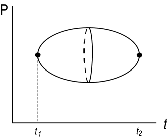
Figure 1: Compact manifolds $\widehat{M}\simeq I\times P$. $I$ is $[t_{1},t_{2}]$ and $P$ is a principal $SO(3)$-bundle over a Quaternionic Kähler manifold. Endpoints at $t_{1}$ and $t_{2}$ are boundaries which can take nut or bolts.

Using the Einstein equation we find the following asymptotic behavior of the metric near the boundary:

1. QK-bolt

   $$a =t/2+a_{3}/6~{}t^{3}+\cdots~{},$$ (4.6)

   $$b =t/2+b_{3}/6~{}t^{3}+\cdots~{},$$

   $$c =t/2+c_{3}/6~{}t^{3}+\cdots~{},$$

   $$f =f_{0}+f_{2}/2~{}t^{2}+\cdots~{}.$$

   Here three of $f_{0}~{},~{}a_{3}~{},~{}b_{3}$ and $c_{3}$ are free parameters which satisfy the relation

   $$a_{3}+b_{3} +c_{3}+\cfrac{n(2+n)}{2f_{0}^{2}}+\frac{1}{2}(1-n)\Lambda=0~{},$$ (4.7)

   and the remaining coefficients are determined by them.

2. T-bolt

   $$a =kt+a_{3}/6~{}t^{3}+\cdots~{},$$ (4.8)

   $$b =c=b_{0}+b_{2}/2~{}t^{2}+\cdots~{},$$

   $$f =f_{0}+f_{2}/2~{}t^{2}+\cdots~{},$$

   where $k\,,\,b_{0}\,,\,f_{0}$ are free parameters and the remaining coefficients are determined by them. The cases $k=2$ and $1/N$ for a positive integer $N$ are exceptional and the expansion above must be modified by the following equations :

   1.  $k=2$

   $$a =2~{}t+a_{3}/6~{}t^{3}+\cdots~{},$$ (4.9)

   $$b =b_{0}+b_{1}~{}t+b_{2}/2~{}t^{2}+\cdots~{},$$

   $$c =b_{0}-b_{1}~{}t+b_{2}/2~{}t^{2}+\cdots~{},$$

   $$f =f_{0}+f_{2}/2~{}t^{2}+\cdots~{},$$

   where $b_{0}\,,\,b_{1}\,,\,f_{0}$ are free parameters and remaining coefficients are determined by these.

   2.  $k=1/N$

   $$a =t/N+a_{3}/6~{}t^{3}+\cdots~{},$$ (4.10)

   $$b =b_{0}+b_{2}/2~{}t^{2}+\cdots~{},$$

   $$c =\sum_{j=0}^{N-1}\frac{b_{2j}}{(2j)!}~{}t^{2j}+\frac{c_{2N}}{(2N)!}~{}t^{2N}+\cdots~{},$$

   $$f =f_{0}+f_{2}/2~{}t^{2}+\cdots~{},$$

   where $b_{0}\,,\,f_{0}\,,\,\delta_{N}=b_{2N}-c_{2N}$ are free parameters and remaining coefficients are determined by these. Derivation of (4.10) is viewed in Appendix B.

3. nut

   $$a =t/2+a_{3}/6~{}t^{3}+\cdots~{},$$ (4.11)

   $$b =t/2+b_{3}/6~{}t^{3}+\cdots~{},$$

   $$c =t/2+c_{3}/6~{}t^{3}+\cdots~{},$$

   $$f =t/2+f_{3}/6~{}t^{3}+\cdots~{},$$

   where $a_{3},~{}b_{3},~{}c_{3}$ and $f_{3}$ are parameters satisfying $a_{3}+b_{3}+c_{3}+4nf_{3}+\Lambda/2=0~{}$.

5 Example

The quaternionic projective space H$P(n)$ is a typical example of QK manifolds. The Hopf fibration $S^{4n+3}\longrightarrow{\mathbf{H}}P(n)$ is a principal $SU(2)$-bundle over H$P(n)$. It has a natural connection such that its horizontal space is the orthogonal complement to the fiber with respect to the standard metric on $S^{4n+3}$. This connection is $c_{1}$-self-dual[17] and in case of $n=1$ the connection is the well-known BPS instanton.

We explicitly calculate the Kaluza-Klein metric based on ${\mathbf{H}}P(n)$ according to sections 2 and 3. For the base space $M$=H$P(n)$, the standard metric is written as

$$g_{M}=\frac{4d\bar{x}^{A}dx^{A}}{1+\bar{x}^{C}x^{C}}-\frac{4\bar{x}^{A}dx^{A}\bar{x}^{B}dx^{B}}{(1+\bar{x}^{C}x^{C})^{2}},$$ (5.1)

where $x^{A}=x_{0}^{A}+x_{1}^{A}i+x_{2}^{A}j+x_{3}^{A}k~{}~{}(A=1\sim n)$ are quaternionic coordinates and $\bar{x}^{A}$ are their conjugates. Then the $c_{1}$-self-dual connection takes the form

$$A^{1}i+A^{2}j+A^{3}k=\frac{\bar{x}^{A}dx^{A}-d\bar{x}^{A}x^{A}}{1+\bar{x}^{B}x^{B}}~{}.$$ (5.2)

Thus we have a Kaluza-Klein metric (2.5) on $I\times P$ explicitly, and the Einstein equation is given by (3.10).

By the construction $P$ is an $SO(3)$-bundle over H$P(n)$. In general, there is an obstruction to lifting an $SO(3)$-bundle over QK manifold to an $SU(2)$-bundle, i.e., the Marchiafava-Romani class $\varepsilon$. A result of [11] says that $\varepsilon=0$ if and only if the QK manifold is H$P(n)$, and so in this case the total space $P$ lifts to the covering space $\tilde{P}$ as an $SU(2)$-bundle. Actually $\tilde{P}$ is the total space of the Hopf fibration, $S^{4n+3}\simeq Sp(n+1)/Sp(n)$.

For completeness we present a summary of the known compact complete metrics based on the Hopf fibration. All these metrics are given as solutions to appropriate reductions of our equation.

1. reduction to one variable ; $a=b=c=f$
   

   $$a(t)=1/2~{}\cos t~{},\quad-\pi/2\leq t\leq\pi/2$$ (5.3)

   with $\Lambda=4n+3~{}$. This solution, which obeys the boundary condition (4.5) at $t=\pm\pi/2~{}$, represents the standard metric on $\widehat{M}=S^{4n+4}~{}$.

2. reduction to two variables ; $a=b=c$ and $f$
   An explicit solution is given by

   $$a(t)=1/2~{}\sin t\cos t~{},\quad f(t)=1/2~{}\cos t~{},\quad 0\leq t\leq\pi/2$$ (5.4)

   with $\Lambda=4n+12~{}$. This solution, which obeys (4.2), (4.5) at $t=0,~{}\pi/2$, respectively, gives the standard metric on ${\mathbf{H}}P(n+1)~{}$. Another solution satisfying (4.2) at the both endpoints was constructed numerically. It gives a metric on an $S^{4}$-bundle over ${\mathbf{H}}P(n)$, i.e., $\widehat{M}={\mathbf{H}}P(n+1)~{}\sharp~{}\overline{{\mathbf{H}}P(n+1)}$[6]. The case $n=1$ has been analytically established by B$\ddot{\mathrm{o}}$hm[18].

3. reduction to two variables ; $a$ and $b=c=f$
   The situation is very parallel to (R2), but the topology is different as we will see shortly. The Fubini-Study metric on C$P(2n+2)$ belongs to this class. Explicitly, the metric is written as

   $$a(t)=1/2~{}\sin t\cos t~{},\quad b(t)=1/2~{}\cos t~{},\quad 0\leq t\leq\pi/2$$ (5.5)

   with $\Lambda=4n+6~{}$. This solution obeys the boundary conditions (4.3), (4.5) at $t=0~{},\pi/2~{}$, respectively. In this case the general solution was constructed by Page-Pope[7] as

   $$\hat{g}=\frac{(1-r^{2})^{2n+1}}{P(r)}dr^{2}+\frac{4m_{1}^{2}P(r)}{(1-r^{2})^{2n+1}}(\phi^{1})^{2}+m_{1}(1-r^{2})g_{Z}~{},$$ (5.6)

   where

   $$P=m_{2}r+\frac{n+1}{m_{1}}Q_{2n+1}-\Lambda~{}Q_{2n+2}~{},\quad Q_{n}=\sum_{j=0}^{n}\binom{n}{j}\frac{(-r^{2})^{j}}{1-2j}$$ (5.7)

   with integration constants $m_{i}$ (i=1,2). Its special case satisfying (4.3) at the both endpoints gives a metric on an $S^{2}$-bundle over the twistor space $Z$, i.e., $\widehat{M}={\mathbf{C}}P(2n+2)~{}\sharp~{}\overline{{\mathbf{C}}P(2n+2)}$ .

6 New Solutions

The solutions listed in the previous section have two of three possible boundaries at the endpoints: (B1) QK-bolt, (B2) T-bolt and (B3) nut. Correspondence between the solutions and boundaries is schematically shown in Fig.2. No solution is found which connects QK-bolt and T-bolt though the existence is naturally expected from the Fig. 2. The solutions with QK-bolt are found in the ansatz (R2), and the solutions with T-bolt are in the other ansatz ($\widetilde{\mathrm{R2}}$), then we search new solutions which connect QK-bolt and T-bolt under a generalized ansatz in which the metric has three unknown variables.

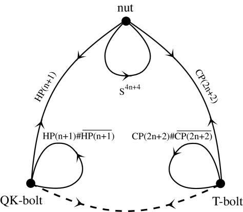
Figure 2: Relation between boundaries and solutions.

We assume $b=c$, hereafter, and treat $a,b,f$ as unknown metric functions of $t$. From (3.10) we obtain the evolution equations

$$\frac{\ddot{a}}{a}=-\frac{\dot{a}}{a}\left(2\frac{\dot{b}}{b}+4n\frac{\dot{f}}{f}\right)+\frac{{a}^{2}}{2\,{b}^{4}}+n\frac{{a}^{2}}{{f}^{4}}-\Lambda,$$ (6.1)

$$\frac{\ddot{b}}{b}=-\frac{\dot{b}}{b}\left(\frac{\dot{a}}{a}+\frac{\dot{b}}{b}+4n\frac{\dot{f}}{f}\right)-\frac{a^{2}-2b^{2}}{2\,{b}^{4}}+n\frac{{b}^{2}}{{f}^{4}}-\Lambda,$$

$$\frac{\ddot{f}}{f}=-\frac{\dot{f}}{f}\left(\frac{\dot{a}}{a}+2\frac{\dot{b}}{b}+(4n-1)\frac{\dot{f}}{f}\right)-\frac{a^{2}+2b^{2}}{2{f}^{4}}+\frac{n+2}{{f}^{2}}-\Lambda.$$

Taking a combination of (3.10) we also get the Hamiltonian constraint

$$2\frac{\dot{b}}{b}\left(2\frac{\dot{a}}{a}+\frac{\dot{b}}{b}\right)+4n\frac{\dot{f}}{f}\left(2\frac{\dot{a}}{a}+4\frac{\dot{b}}{b}+(4n-1)\frac{\dot{f}}{f}\right)$$ (6.2)

$$\hskip 28.45274pt+\frac{{a}^{2}-4{b}^{2}}{2{b}^{4}}+n\frac{a^{2}+2b^{2}}{f^{4}}-4n(n+2)\frac{1}{f^{2}}+(4n+2)\Lambda=0.$$ (6.3)

We should integrate the equations (6.1) from QK-bolt at $t=t_{1}=0$ as an ‘initial’ value problem in $t$. Since $a$ and $b$ are zero at $t=0$, the set of ordinary differential equations (6.1) is singular there. To deal with the singularity, we use the asymptotic form of the solutions (4.6) near the singularity, and start numerical integrations at an initial time $t=t_{i}=0+\epsilon$, where $\epsilon$ is a small amount of time duration.

Equation (4.6) gives the asymptotic behavior of $a,b$ and $f$ near QK-bolt:

$$a =t/2+a_{3}/6~{}t^{3}+\cdots~{},$$ (6.4)

$$b =t/2+b_{3}/6~{}t^{3}+\cdots~{},$$

$$f =f_{0}+f_{2}/2~{}t^{2}+\cdots~{},$$

where $f_{0},~{}a_{3}$ and $b_{3}$ satisfy

$$a_{3}+2b_{3}+\cfrac{n(2+n)}{2f_{0}^{2}}+\frac{1}{2}\left(1-n\right)\Lambda=0~{},$$ (6.5)

and $f_{2}$ is given by

$$f_{2}=\frac{1}{4}\left(\frac{n+2}{f_{0}}-\Lambda f_{0}\right).$$ (6.6)

Introducing a parameter $g_{0}$ by

$$g_{0}=\frac{1}{3}(b_{3}-a_{3}),$$ (6.7)

we can solve (6.5) as

$$a_{3}=\frac{1}{6}(n-1)\Lambda-\frac{n}{6}(n+2)\frac{1}{f_{0}^{2}}-2g_{0},$$ (6.8)

$$b_{3}=\frac{1}{6}(n-1)\Lambda-\frac{n}{6}(n+2)\frac{1}{f_{0}^{2}}+g_{0}.$$

Therefore, the initial condition at $t=t_{i}$ is given by (6.4) (6.6) and (6.8) with $t=\epsilon$. We have two free parameters $f_{0}$ and $g_{0}$ to specify the initial condition near QK-bolt.

We are interested in finding solutions for which $b$ and $f$ stay positive and finite, and $a$ returns to zero at some moment $t=t_{2}$. At this point the set of equations (6.1) becomes singular again. We assume that this singularity is resolved by T-bolt (4.3). If $k\neq 1$ the cone-type singularity appears at $t=t_{2}$ so we set $k=1$ for regularity. Then the condition (4.10) with $b=c$ ($\delta_{1}=0$) shows that the asymptotic behavior of $a,b$ and $f$ near $t=t_{2}$ should be

$$a = (t_{2}-t)+\bar{a}_{3}/6~{}(t_{2}-t)^{3}+\cdots~{},$$ (6.9)

$$b = \bar{b}_{0}+\bar{b}_{2}/2~{}(t_{2}-t)^{2}+\cdots~{},$$ (6.10)

$$f = \bar{f}_{0}+\bar{f}_{2}/2~{}(t_{2}-t)^{2}+\cdots,$$ (6.11)

where $\bar{b}_{0}$ and $\bar{f}_{0}$ are free constants and $\bar{a}_{3},\bar{b}_{2}$ and $\bar{f}_{2}$ are described by them as

$$\bar{a}_{3} =-\frac{1}{\bar{b}_{0}^{2}}+n\frac{\bar{b}_{0}^{2}}{\bar{f}_{0}^{4}}-\frac{2n(n+2)}{\bar{f}_{0}^{2}}+2n\Lambda~{},$$ (6.12)

$$\bar{b}_{2} =\frac{\bar{b}_{0}}{2}~{}\left(\frac{1}{\bar{b}_{0}^{2}}+n\frac{\bar{b}_{0}^{2}}{\bar{f}_{0}^{4}}-\Lambda\right)~{},$$

$$\bar{f}_{2} =\frac{\bar{f}_{0}}{2}~{}\left(-\frac{\bar{b}_{0}^{2}}{\bar{f}_{0}^{4}}+\frac{2+n}{\bar{f}_{0}^{2}}-\Lambda\right)~{}.$$

We stop numerical integrations at $t_{f}=t_{2}-\bar{\epsilon}$ ($\bar{\epsilon}$ is a small constant) and check whether the values of $a,b,f$ and $\dot{a},\dot{b},\dot{f}$ agree with (6.9)-(6.11).

Here, we define

$$V^{1}=\dot{a}(t_{f})-\dot{a}_{T},$$ (6.13)

$$V^{2}=\dot{b}(t_{f})-\dot{b}_{T},$$

where

$$\dot{a}_{T}=-1-\bar{a}_{3}/2~{}\bar{\epsilon}^{2},\quad\dot{b}_{T}=-\bar{b}_{2}~{}\bar{\epsilon}.$$ (6.14)

A solution for (6.1) defined on the region $[t_{i},t_{f}]$ gives a map $\{(f_{0},g_{0})\}\rightarrow\{(V^{1},V^{2})\}$. Then we can regard $V=(V^{1},V^{2})$ as a vector field on a 2-dimensional plane parameterized by $(f_{0},g_{0})$. If $V=0$, $a$ and $b$ have the forms of (6.9) and (6.10) near $t=t_{2}$, in addition, it is shown from (6.3) $f$ should have the form of (6.11) automatically. Then, vanishing of $V$ means the endpoint at $t=t_{2}$ is T-bolt.

Numerical integrations are done by using a fourth-order Runge-Kutta routine. We have verified that the constraint (6.3), which is preserved by the evolution equations (6.1), holds in high accuracy in our numerical integrations. We also reproduce known solutions listed in the previous section when we set $a=b$ or $b=f$.

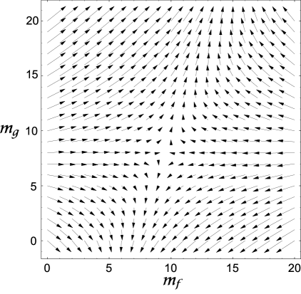
Figure 3: Vector field $V$ on $(f_{0},g_{0})$-plane for $n=1$ case. Parameters $m_{f}$ and $m_{g}$ give $f_{0}$ and $g_{0}$ as $f_{0}=1.75333405+1.0\times 10^{-8}\times m_{f}$ and $g_{0}=0.002532820+1.0\times 10^{-9}\times m_{g}$. Horizontal and vertical components of the arrows are $V^{1}$ and $V^{2}$, respectively. The vector field vanishes on a point $(f_{0}^{*},g_{0}^{*})\sim(1.75334014,0.002532828)$.

Fig.3 shows the vector field $V$ on $(f_{0},g_{0})$-plane for $n=1$ case. We normalize $\Lambda=1$. There is a critical point $(f_{0}^{*},g_{0}^{*})$ on which $V$ vanishes. The map $(f_{0}^{*},g_{0}^{*})\mapsto V=0$ corresponds to the solution for (6.1) which connects QK-bolt at $t=0$ and T-bolt at $t=t_{2}$. Evolution of $a,b$ and $f$ in $t$ is plotted in Fig.4.

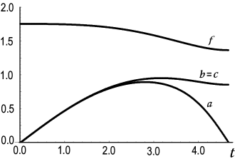
Figure 4: Evolution of $a,b$ and $f$ in $t$ for the critical point $(f_{0}^{*},g_{0}^{*})$ in $n=1$ case.

$n$	$\sqrt{n+2}$	$f_{0}^{*}$	$g_{0}^{*}$	$\bar{f}_{0}$	$\bar{b}_{0}$	$f_{0}^{*}-\bar{f}_{0}$	$t_{2}-t_{1}$
1	1.73205	1.75334	0.00253	1.36425	0.85289	0.38910	4.65747
2	2.00000	2.05472	0.00441	1.74912	0.97181	0.30559	4.49746
3	2.23607	2.30830	0.00633	2.03541	1.04715	0.27290	4.37347
4	2.44949	2.52917	0.00811	2.27774	1.10000	0.25143	4.28367
5	2.64575	2.72822	0.00968	2.49323	1.13927	0.23499	4.21713
6	2.82843	2.91144	0.01107	2.68983	1.16969	0.22161	4.16625
14	4.00000	4.07213	0.01767	3.91020	1.28394	0.16193	3.98370
23	5.00000	5.06126	0.02091	4.93003	1.32869	0.13122	3.91686
47	7.00000	7.04587	0.02420	6.95105	1.36954	0.09482	3.85836
98	10.00000	10.03288	0.02616	9.96609	1.39204	0.06679	3.82719
223	15.00000	15.02219	0.02726	14.97751	1.40431	0.04468	3.81052
898	30.00000	30.01117	0.02795	29.98879	1.41173	0.02238	3.80052
2498	50.00000	50.00671	0.02810	49.99328	1.41333	0.01344	3.79839
9998	100.00000	100.00336	0.02816	99.99664	1.41399	0.00672	3.79749
999998	1000.00000	1000.00034	0.02818	999.99966	1.41421	0.00067	3.79719

Table 1: Numerical parameters for $(4n+4)$-dimensional solutions. Parameters $f_{0}^{*},g_{0}^{*}$ for compact solutions, and parameters $\bar{f}_{0},\bar{b}_{0}$, the difference $f_{0}^{*}-\bar{f}_{0}$, and the interval $t_{2}-t_{1}$ are listed. The cosmological constant is normalized as unity.

The vectors $V$ in Fig.3 turn $2\pi$ in the direction along a circle around the critical point $(f_{0}^{*},g_{0}^{*})$. Since the right hand sides of (6.1) are regular in $t\in[t_{i},t_{f}]$, the components of $V$ are continuous functions with respect to $(f_{0},g_{0})$. Then there definitely exists a critical point on which $V=0$ inside the circle. Therefore this figure strongly suggests the existence of the solution with both QK-bolt and T-bolt.

As commented in section 5, the numerical metric with $k=1$ extends over the QK manifold $M$ with an orbifold singularity at $t=0$, and extends smoothly over the twistor space $Z$ at the other endpoint $t=t_{2}$. If we allow the cone-like singularity at T-bolt, $k$ can take an arbitrary value. The case is commented shortly in Appendix B.

In table 1 we list numerical values $f_{0}^{*}$ and $g_{0}^{*}$ for compact solutions of various dimensions $4n+4$ of the manifold. As $n$ is increased, $f(t)$ stays almost constant around $\sqrt{n+2}$ over the range of $t$, and the value of $\bar{b}_{0}$ at $t_{2}$ and the interval of the numerical solutions $t_{2}-t_{1}$ converges. Though the scale of the base space $f$ diverges in the order of $\sqrt{n}$ it seems that the 4-dimensional fiber metric converges. It should be noted that during the evolutions $\dot{f}/f$ is very small for large $n$ but the terms $4n\dot{f}/f$ in (6.1) contribute in the same order of $\dot{a}/a$ and $\dot{b}/b$.

7 Summary and Discussion

In the present work, we have made an investigation of higher dimensional compact Einstein manifolds. We can view such manifolds as the union of principal $SO(3)$-bundles over Quaternionic Kähler manifolds. Globally, our compact manifold $\widehat{M}$ is considered as a fiber bundle associated with a principal $G$-bundle $P$, i.e., $\widehat{M}=P\times_{G}F$  ($G=SO(3)$ or $SU(2)$) . The fiber $F$ is a 4-dimensional manifold (orbifold) with the Bianchi IX metric on which $G$ acts with cohomogeneity one, and the base space $M$ is the Quaternionic Kähler manifold.

Total space $\widehat{M}$ can be regarded as an evolution of $P$ over a finite ‘time’ segment $[t_{1},t_{2}]$. If we require the compactness, singularities at the boundaries $t_{1}$ and $t_{2}$ should be resolved by nut, Quaternionic Kähler(QK)-bolt or Twistor(T)-bolt. We found new solutions numerically which connect QK-bolt and T-bolt in the present paper, where T-bolt is characterized by a number $k$. To the extent of the three unknown variables $a,b=c,f$ for the metric form (2.5), we could complete Fig.2 by using the new solutions (broken line) and already known solutions (solid lines).

Since $\widehat{M}$ has the bundle structure with the fiber $F$ on the base space $M$ then the Euler number is factorized as

$$\chi(\widehat{M})=\chi(M)\chi(F)~{}.$$ (7.1)

By using the Gauss-Bonnet theorem, $\chi(F)$ is calculated as

$$\chi(F) =\frac{1}{32\pi^{2}}\int_{F}\varepsilon_{abcd}~{}\Omega_{ab}\wedge\Omega_{cd} =N_{G}(1/2+2k)~{},$$ (7.2)

where $N_{G}=1$ if $G=SO(3)$ and $N_{G}=2$ if $G=SU(2)$. The factors 1/2 and $2k$ in (7.2) represent the contribution from QK and T-bolts, respectively.

Let us consider the large $n$ limit. Though the scale of the base space $f$ diverges in the order of $\sqrt{n}$ the coefficients (6.8) of the local expansion near QK-bolt become

$$a_{3}=-2g_{0}^{*}-\Lambda/6~{},\quad b_{3}=g_{0}^{*}-\Lambda/6$$ (7.3)

and the ones (6.12) near T-bolt become

$$\bar{a}_{3}=-\frac{1}{\bar{b}_{0}^{2}},\quad b_{2}=\frac{1}{2\bar{b}_{0}}-\frac{\bar{b}_{0}}{2}\Lambda,$$ (7.4)

which might imply that the fiber metric converges to the 4-dimensional biaxial Bianchi IX metric

$$g_{\infty}=dt^{2}+\tilde{a}(t)^{2}\sigma_{1}^{2}+\tilde{b}(t)^{2}(\sigma_{2}^{2}+\sigma_{3}^{2})$$ (7.5)

in the limit $n\rightarrow\infty$.

When the total space connects QK-bolt and T-bolt, the fiber space with the metric (7.5) connects nut and bolt in 4-dimensions. It is known that the 4-dimensional biaxial Bianchi IX Einstein metrics connecting nut and bolt singularities is either the self-dual Taub-NUT-de Sitter metric or the self-dual Eguchi-Hanson-de Sitter metric, and their common boundary represents the Fubini-Study metric on ${\mathbf{C}}P(2)$[19]. A question is whether the fiber metric coincides with the Bianchi IX Einstein metric in the limit $n\rightarrow\infty$. Indeed the expansion (7.3) locally reproduces the behavior of the self-dual Eguchi-Hanson-de Sitter metric near the nut singularity, but the global metric is different since the value $k=1$ at the other endpoint (bolt singularity) for the fiber metric is not allowed for the 4-dimensional solution.

This situation can be compared with the metric on ${\mathbf{H}}P(n+1)~{}\sharp~{}\overline{{\mathbf{H}}P(n+1)}$ solved by Page and Pope[6] in the ansatz (R1) ; in the large $n$ limit, $f$ stays constant and the fiber metric gives the standard $S^{4}$ metric i.e., the full metric approaches the direct product Einstein metric. In contrast, the numerical metric presented here is not the direct product metric even in the large $n$ limit, where the existence of the gauge field $A^{i}$ is important.

Finally we discuss the relation to the $Spin(7)$ holonomy metrics. In the beautiful papers[20][21] Hitchin constructed a family of 4-dimensional self-dual Einstein metrics with positive Ricci curvature in a triaxial Bianchi IX form parameterized by an integer $N$. These solutions connect the two bolt singularities characterized by $k=2$ and by $1/N$. The metrics are explicitly given by the solution to the Painlevé VI equation[23] and approach the Atiyah-Hitchin hyperkähler metric[22] with $Sp(1)$ holonomy in the limit $N\rightarrow\infty$.

In 8-dimensional case, the asymptotically locally conical (ALC) $Spin(7)$ metrics would be counterparts of the Atiyah-Hitchin metric[13, 24, 25]. The local behavior (4.9) at T-bolt with $k=2$ reproduces the ALC $Spin(7)$ metric when one of the free parameters is adjusted suitably. Furthermore the expansion (4.10) of the fiber metric at the other T-bolt with $k=1/N$ has the same form as the Hitchin metrics. It is tempting to expect that there is a series of Einstein metrics with positive Ricci curvature in 8-dimensions which approach the ALC $Spin(7)$ metric in a suitable large $N$ limit. Therefore, it is interesting to consider solutions in the general metric form (2.5) which connect two T-bolt singularities, $k=2$ and $1/N$. We leave this issue for further research.

Acknowledgements

We would like to thank H.Kanno for helpful discussions. This work is supported in part by the Grant-in-Aid for Scientific Research No.14540275 and No. 14570073.

Appendix A

In this appendix we calculate the Ricci tensor of the off-diagonal metric (2.4) . When we use the basis $\phi^{i}\,(i=1\sim 3)$ for the fiber metric and the orthonormal basis $\hat{e}^{0}\,,\hat{e}^{\alpha}\,\,(\alpha=1\sim m)$ defined by (2.6) , the non-zero components are

$$\widehat{R}_{00} =-\sum_{i}\dot{K}^{i}_{i}-\sum_{i,j}K^{j}_{i}K^{i}_{j}-m\cfrac{\ddot{f}}{f}~{},$$ (A.1)

$$\widehat{R}_{ij} =-\sum_{k}\dot{K}^{k}_{i}b_{kj}-\left(\sum_{\ell}K^{\ell}_{\ell}+m\cfrac{\dot{f}}{f}\right)\sum_{k}K^{k}_{i}b_{kj}$$

$$+R^{SO(3)}_{ij}+\cfrac{1}{4f^{4}}\sum_{k,\ell,m,n}\sum_{\alpha,\gamma}b_{ik}b_{j\ell}{\mathcal{O}}_{mk}F^{m}_{\alpha\gamma}{\mathcal{O}}_{n\ell}F^{n}_{\alpha\gamma}~{},$$

$$\widehat{R}_{\alpha\beta} =-\left(\cfrac{\ddot{f}}{f}+(m-1)\cfrac{\dot{f}^{2}}{f^{2}}+\sum_{i}K^{i}_{i}\cfrac{\dot{f}}{f}\right)\delta_{\alpha\beta}$$

$$+\cfrac{1}{f^{2}}R_{\alpha\beta}-\cfrac{1}{2f^{4}}\sum_{ijk\ell}\sum_{\gamma}b_{ij}{\mathcal{O}}_{ki}F^{k}_{\alpha\gamma}{\mathcal{O}}_{\ell j}F^{\ell}_{\beta\gamma}~{},$$

$$\widehat{R}_{0i} =-\sum_{jk}\varepsilon_{ijk}K^{k}_{j}~{},$$

$$\widehat{R}_{i\alpha} =\cfrac{1}{2f^{3}}\sum_{jk}\sum_{\beta}b_{ij}{\mathcal{O}}_{kj}D_{\beta}F^{k}_{\alpha\beta}~{}.$$

Here $K^{j}_{i}=(1/2)\dot{b}_{ik}b^{kj}$ and $R^{SO(3)}_{ij}$ denotes the Ricci tensor on $SO(3)$ ;

$$R^{SO(3)}_{ij} =-\sum_{k\ell}\Gamma^{k}_{i\ell}\Gamma^{\ell}_{jk}~{},\quad\Gamma^{k}_{ij} =\cfrac{1}{2}\left(\varepsilon_{ijk}+\sum_{\ell m}\varepsilon_{i\ell m}b_{mj}b^{k\ell}+\sum_{\ell m}\varepsilon_{j\ell m}b_{mi}b^{k\ell}\right)~{}.$$ (A.2)

When we impose the assumption of 4n-dimensional QK manifolds (see section 3) , then $\widehat{R}_{i\alpha}=0$ and the explicit dependence of the group element ${\mathcal{O}}_{ij}$ disappears from the equations,

$$\sum_{k,\ell,m,n}\sum_{\alpha,\gamma}b_{ik}b_{j\ell}{\mathcal{O}}_{mk}F^{m}_{\alpha\gamma}{\mathcal{O}}_{n\ell}F^{n}_{\alpha\gamma} =4n\sum_{k}b_{ik}b_{kj}~{},$$ (A.3)

$$\sum_{ijk\ell}\sum_{\gamma}b_{ij}{\mathcal{O}}_{ki}F^{k}_{\alpha\gamma}{\mathcal{O}}_{\ell j}F^{\ell}_{\beta\gamma} =\sum_{i}b_{ii}\delta_{\alpha\beta}~{},$$

which yields the $SO(3)$ invariance of the Einstein equation.

Appendix B

Putting $y=b-c$, and then using the Einstein equation (3.10) we obtain

$$\ddot{y}=p\dot{y}+qy~{},$$ (B.1)

where the coefficients $p$ and $q$ are given by

$$p =-\frac{\dot{a}}{a}-4n\frac{\dot{f}}{f}~{},$$ (B.2)

$$q =-\frac{\dot{b}\dot{c}}{bc}-\frac{1}{2a^{2}b^{2}c^{2}}(a^{2}-b^{2}-c^{2})(a^{2}+b^{2}+2bc+c^{2})$$

$$+\frac{n}{f^{4}}(b^{2}+bc+c^{2})-\Lambda~{}.$$

Taking account of the expansion (LABEL:ex1), we approximate the equation (B.1) in the limit $t\rightarrow 0$,

$$\ddot{y}+\frac{1}{t}\dot{y}-\frac{4N^{2}}{t^{2}}y=0,$$ (B.3)

which has the regular solution $y=t^{2N}$ for a positive integer $N$. Thus we conclude that the expansion takes the form of (4.10).

Appendix C

Let us consider $k\neq 1$ case, where cone-like singularity appears at T-bolt. The angle around T-bolt is $2\pi k$ then the singularity is angular deficit for $k<1$ and angular excess for $k>1$. In this case, solutions make a family parameterized by $k$. A curve on the $(f_{0},g_{0})$-plane depicted in Fig. 5 shows a family of solutions.

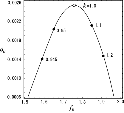
Figure 5: The curve on $(f_{0},g_{0})$-plane which denotes a family of solutions with a cone-like singularity in $n=1$ case. The open circle on the curve, critical point $(f_{0}^{*},g_{0}^{*})$, is the solution with $k=1$, which is regular at T-bolt. The left branch with respect to the critical point corresponds to the solutions with angular deficit and the right branch does angular excess.