KOBE-TH 03-03

TIT/HEP-496

OU-HET-444/2003

Phase Structures of $SU(N)$ Gauge-Higgs Models
on
Multiply Connected Spaces

Hisaki Hatanaka^(a), Katsuhiko Ohnishi^(b), , Makoto Sakamoto^(c), and

Kazunori Takenaga^(d),

^(a) Department of Physics, Tokyo Institute of Technology, Tokyo 152-8551, Japan

^(b)Graduate School of Science and Technology, Kobe University,
Rokkodai, Nada, Kobe 657-8501, Japan

^(c) Department of Physics, Kobe University, Rokkodai, Nada, Kobe 657-8501, Japan

^(d) Department of Physics, Osaka University, Toyonaka, Osaka 560-0043, Japan

We study an $SU(N)$ gauge-Higgs model with $N_{F}$ massless fundamental fermions on $M^{3}\otimes S^{1}$. The model has two kinds of order parameters for gauge symmetry breaking: the component gauge field for the $S^{1}$ direction (Hosotani mechanism) and the Higgs field (Higgs mechanism). We find that the model possesses three phases called Hosotani, Higgs and coexisting phases for $N=$ odd, while for $N=$ even, the model has only two phases, the Hosotani and coexisting phases. The phase structure depends on a parameter of the model and the size of the extra dimension. The critical radius and the order of the phase transition are determined. We also consider the case that the representation of matter fields under the gauge group is changed. We find some models, in which there is only one phase independent of parameters of the models as well as the size of the extra dimension.

1 Introduction

Recently, physics with extra dimensions has been studied extensively in connection with the long standing problems, namely, new mechanism and/or the origin of (gauge, super) symmetry breaking in elementary particle physics. It can provide us new insight and understanding for low-energy physics. In fact, it has been pointed out[1] that new mechanism of spontaneous supersymmetry breaking is possible in a certain class of models as a consequence of the breakdown of the translational invariance for the extra dimension $S^{1}$[2, 3]. Furthermore, one of our authors (M.S) and his collaborators have shown[4] that the rotational invariance of $S^{2}$ is spontaneously broken in a monopole background above some critical radius due to the appearance of vortex configuration as vacuum configuration.

When one considers gauge-Higgs models on space-time with some of the space directions being compactified on a multiply connected space, one should take account of gauge symmetry breaking through the Hosotani mechanism[6]. The mechanism essentially occurs due to quantum corrections in the extra dimension, reflecting the topology of the compactified space. It is possible for the component gauge field for the compactified direction to acquire nonvanishing vacuum expectation values (VEV). The Hosotani mechanism has been studied extensively in (supersymmetric) gauge models[7, 8, 9, 10, 12, 13, 11] and, in particular, paid much attention in the context of orbifold compactifications[14, 15]. On the other hand, the Higgs mechanism also breaks gauge symmetry by the nonvanishing VEV for the Higgs field even at the tree level. This suggests that if we consider the gauge-Higgs model on such the space-time, the gauge symmetry can be broken by both or either of the two mechanisms due to the existence of the two kinds of the order parameters for gauge symmetry breaking.

In a previous paper[16] we showed that phase structures of gauge-Higgs models on $M^{3}\otimes S^{1}$ are nontrivial, where $M^{3}(S^{1})$ is three-dimensional Minkowski space-time (a circle). In the paper we studied the phase structure of the simplest $SU(2)$ gauge-Higgs model and found three different phases called Hosotani, Higgs and coexisting phases. In each phase the VEVs for the two order parameters take the different forms and values. The structure depends on a parameter of the model and the size of $S^{1}$. The critical radius and the order of the phase transition were determined explicitly. We also pointed out that the phase structure could provide a new approach to the gauge hierarchy problem in grand unified theory (GUT).

This paper is a generalization of the previous work. In particular, we shall investigate the phase structure of an $SU(N)$ gauge-Higgs model with $N_{F}$ massless fermions on $M^{3}\otimes S^{1}$. In the next section we analyze the phase structure of the model, in which both the fermion and Higgs fields belong to the fundamental representation under $SU(N)$. We will find that the phase structure of the model is very different, depending on whether $N$ is even or odd. For the case $N=$ odd, there are the three phases, and the structure is similar to the one obtained in the previous paper. Only two phases, the Hosotani and the coexisting phases, appear for $N=$ even, and the Higgs phase does not exist for finite sizes of the extra dimension. We also determine the critical radius and the order of the phase transition. In the models, the Hosotani mechanism works as the restoration of the gauge symmetry. In Sec. $3$, we consider the case that the representation of matter fields under the gauge group is changed. We find some models whose phase structures do not depend on the parameters of the models and also the size of the extra dimension. The final section is devoted to conclusions and discussions. Details of calculations will be given in Appendix.

2 $SU(N)$ Gauge-Higgs Model

We study the vacuum structure of an $SU(N)$ gauge-Higgs model with $N_{F}$ massless fundamental fermions. The Higgs field also belongs to the fundamental representation under $SU(N)$. We take our space-time to be $M^{3}\otimes S^{1}$ in order to perform analytic calculations, where $M^{3}$ and $S^{1}$ stand for three-dimensional Minkowski space-time and a circle with radius $R$, respectively. Our action is

$$S=\int d^{3}x\int_{0}^{L}dy\left(-{1\over 2}{\rm tr}F_{\hat{\mu}\hat{\nu}}F^{\hat{\mu}\hat{\nu}}+\sum_{I=1}^{N_{F}}{\bar{\psi}}_{I}i\Gamma^{\hat{\mu}}D_{\hat{\mu}}\psi_{I}+(D^{\hat{\mu}}\Phi)^{\dagger}D_{\hat{\mu}}\Phi-V(\Phi^{\dagger},\Phi)\right),$$ (1)

where the Higgs potential is given by

$$V(\Phi^{\dagger},\Phi)=-m^{2}\Phi^{\dagger}\Phi+{\lambda\over 2}(\Phi^{\dagger}\Phi)^{2}.$$ (2)

We have used a notation such as $x^{\hat{\mu}}\equiv(x^{\mu},y)$ and the length of the circumference of $S^{1}$ by $L=2\pi R$.

As stated in the introduction, there are two kinds of the order parameters for gauge symmetry breaking. One is the component gauge field $A_{y}$ for the $S^{1}$ direction, which is related with the Hosotani mechanism, and the mechanism is essentially caused by quantum corrections in the extra dimension. The other one is the Higgs field, and the Higgs mechanism works even at the tree-level. Taking the order parameters into account, we study the effective potential for $\langle A_{y}\rangle$ and $\langle\Phi\rangle$ parametrized by

$$gL\langle A_{y}\rangle={\rm diag}(\theta_{1},\theta_{2},\cdots,\theta_{N}),~{}~{}\langle\Phi\rangle={1\over\sqrt{2}}(v,0,\cdots,0)^{T},$$ (3)

where $\sum_{i=1}^{N}\theta_{i}=0$ and $v$ is a real constant. Here, we have arranged $\theta_{i}$ in such a way that ${\left|{\hat{\theta}_{1}}\right|}\leq{\left|{\hat{\theta}_{2}}\right|}\leq\cdots\leq{\left|{\hat{\theta}_{N}}\right|}$, where $\hat{\theta}_{i}=\theta_{i}$ mod $2\pi$ with $\hat{\theta}_{i}\leq\pi$. This can be done without loss of generality. We showed in the appendix that the parametrization for the vacuum expectation value (VEV) of the Higgs field given in Eq.(3) is enough to study the vacuum structure of the model. We assume $N_{F}$ is so large that the leading order correction comes from the fermion one-loop correction to $\langle A_{y}\rangle$ alone. Then, the effective potential is given by

$$V = -{1\over 2}m^{2}v^{2}+{\lambda\over 8}v^{4}+{{\hat{\theta}_{1}^{2}v^{2}}\over{2L^{2}}}+{A\over{\pi^{2}L^{4}}}\sum_{n=1}^{\infty}\sum_{i=1}^{N}{1\over n^{4}}\cos(n\theta_{i})$$ (4)

$$= {1\over L^{4}}\left(-{1\over 2}\bar{m}^{2}\bar{v}^{2}+{\lambda\over 8}\bar{v}^{4}+{1\over 2}\hat{\theta}_{1}^{2}\bar{v}^{2}+{A\over{\pi^{2}}}\sum_{n=1}^{\infty}\sum_{i=1}^{N}{1\over n^{4}}\cos(n\theta_{i})\right)\equiv\bar{V}L^{-4},$$ (5)

where $A\equiv 2^{2}N_{F}$ and the number $2^{2}$ counts the physical degrees of freedom of a Dirac fermion. Here, we have introduced the dimensionless quantities, $\bar{m}\equiv mL,\bar{v}\equiv vL$. The first two terms in Eq. (4) are nothing but the classical Higgs potential, and the third term comes from the interaction between the gauge and Higgs fields in $D_{y}\Phi$, which, as we will see later, plays an important role to determine the phase structure of the model. The fourth term stands for the one-loop correction from the fermions. We have neglected other one-loop corrections arising from the gauge and Higgs fields under the assumption that the number of the fermions $N_{F}$ is sufficiently large and also that the couplings $g$ and $\lambda$ are sufficiently small. We make use of the assumption throughout the paper.

If we look at the dependence of the effective potential on the scale $L$ in Eq.(4), it suggests that the vacuum structure changes according to the size of the extra dimension. When $L$ is large enough, the quantum correction in the extra dimension is suppressed and the leading order contribution is given by the classical Higgs potential, so that the Higgs field acquires the nonvanishing VEV. The next leading order contribution, the third term in Eq.(4), yields vanishing $\hat{\theta}_{1}$ in order to minimize the potential in the large $L$ limit. On the other hand, if $L$ is small enough, the quantum correction in the extra dimension dominates the effective potential, and we would obtain nonzero values of $\theta_{i}$. Then, the next leading order term, the third term, would enforce to result in $v=0$. This simplified discussion implies that the vacuum structure depends on the size of the extra dimension. One, of course, needs to study the effective potential carefully in order to determine the vacuum structure of the model.

Let us now study the vacuum structure of the model. We follow the standard procedure to find the vacuum configuration. We first solve equations of the first derivative of the effective potential (5) with respect to the order parameters,

$${{\partial\bar{V}}\over{\partial\bar{v}}} = \bar{v}\left(-\bar{m}^{2}+{\lambda\over 2}\bar{v}^{2}+\hat{\theta}_{1}^{2}\right)=0,$$ (6)

$${{\partial\bar{V}}\over{\partial\theta_{1}}} = \hat{\theta}_{1}\bar{v}^{2}+{A\over\pi^{2}}\sum_{n=1}^{\infty}{{-1}\over n^{3}}\left(\sin(n\theta_{1})+\sin(n\sum_{i=1}^{N-1}\theta_{i})\right)=0,$$ (7)

$${{\partial\bar{V}}\over{\partial\theta_{k}}} = {A\over\pi^{2}}\sum_{n=1}^{\infty}{{-1}\over n^{3}}\left(\sin(n\theta_{k})+\sin(n\sum_{i=1}^{N-1}\theta_{i})\right)=0,\quad k=2,\cdots,N-1,$$ (8)

where we have used $\theta_{N}=-\sum_{i=1}^{N-1}\theta_{i}$. Solutions to the equations are candidates of the vacuum configuration. Then, we analyze the stability of the solutions against small fluctuations, and this constrains allowed regions of the solutions as the local minimum of the effective potential. Among various, if any, candidates of those configurations, the global minimum of the effective potential is given by the configuration which gives the lowest energy. Following these steps, one can obtain the vacuum structure of the model.

The equation (6) leads to

$$\bar{v}=0,$$ (10)

$${\rm or}$$

$$-\bar{m}^{2}+{\lambda\over 2}\bar{v}^{2}+\hat{\theta}_{1}^{2}=0.$$

For the first case (10), the equations (7) and (8) are unified into an equation,

$${A\over\pi^{2}}\sum_{n=1}^{\infty}{{-1}\over n^{3}}\left(\sin(n\theta_{k})+\sin(n\sum_{i=1}^{N-1}\theta_{i})\right)=0,\quad k=1,\cdots,N-1.$$ (11)

We call the solution to this equation type I, and the solution describes the Hosotani phase. On the other hand, for the second case (10) we solve the coupled equations,

$${2\over\lambda}(\bar{m}^{2}-\hat{\theta}_{1}^{2})\hat{\theta}_{1}+{A\over\pi^{2}}\sum_{n=1}^{\infty}{{-1}\over n^{3}}\left(\sin(n\theta_{1})+\sin(n\sum_{i=1}^{N-1}\theta_{i})\right) = 0,$$ (12)

$${A\over\pi^{2}}\sum_{n=1}^{\infty}{{-1}\over n^{3}}\left(\sin(n\theta_{k})+\sin(n\sum_{i=1}^{N-1}\theta_{i})\right) = 0,\quad k=2,\cdots,N-1.$$ (13)

A solution to the equation is called type II or type III, depending on whether the solution has the scale dependence on the extra dimension or not. The type II (III) corresponds to the Higgs (coexisting) phase, whose vacuum expectation values are independent of (dependent on) the scale of the extra dimension. In order to avoid unnecessary complexity, details of calculations to solve these equations will be given in the appendix. We find that it is convenient to discuss the vacuum structure separately, depending on whether $N$ is odd or even. Let us first study the case $N=$ odd.

2.1 $N=$ odd

There are three types of possible vacuum configurations, as shown in the appendix,

$${\rm type~{}~{}I} \cdots \left\{\begin{array}[]{l}gL\langle A_{y}\rangle={\rm diag}\left({{N-1}\over N}\pi,\cdots,{{N-1}\over N}\pi,-{{(N-1)^{2}}\over N}\pi\right),\\[8.5359pt] \langle\Phi\rangle={1\over\sqrt{2}}(0,\cdots,0)^{T},\end{array}\right.$$ (16)

$${\rm type~{}~{}II} \cdots \left\{\begin{array}[]{l}gL\langle A_{y}\rangle={\rm diag}\left(0,\pi,\pi,\cdots,-(N-2)\pi\right),\\[8.5359pt] \langle\Phi\rangle={1\over\sqrt{2}}(\sqrt{2\over\lambda}m,0,\cdots,0)^{T},\end{array}\right.$$ (19)

$${\rm type~{}~{}III} \cdots \left\{\begin{array}[]{l}gL\langle A_{y}\rangle={\rm diag}\left(\theta_{1}^{-},\pi-{\theta_{1}^{-}\over{N-1}},\cdots,\pi-{\theta_{1}^{-}\over{N-1}},-((N-2)\pi+{\theta_{1}^{-}\over{N-1}})\right),\\[8.5359pt] \langle\Phi\rangle={1\over\sqrt{2}}(v,\cdots,0)^{T}.\end{array}\right.$$ (22)

The type III solution depends on the scale $\bar{m}$, and accordingly, $\bar{v}=\sqrt{{2\over\lambda}(\bar{m}^{2}-(\theta_{1}^{-})^{2})}$ does as well. The explicit form of $\theta_{1}^{-}(\bar{m})$ is given by Eq.(93) in the appendix. As we stated before, we call the vacuum configuration corresponding to the type I, II and III solutions the Hosotani, Higgs and coexisting phases, respectively.

Given the vacuum configuration, the gauge symmetry in each phase is generated by the generators $T^{a}$ of $SU(N)$ which commute with the Wilson line,

$$W\equiv{\cal P}{\rm exp}\left(ig\oint_{S^{1}}dy\langle A_{y}\rangle\right)={\rm diag}\left({\rm e}^{i\theta_{1}},{\rm e}^{i\theta_{2}},\cdots,{\rm e}^{i\theta_{N}}\right)\quad{\rm and}\quad T^{a}\langle\Phi\rangle=0.$$ (23)

Let us note that the phase $\theta_{i}$ is defined modulo $2\pi$. It is easy to observe that the $SU(N)$ gauge symmetry is not broken in the Hosotani phase because the Wilson line for the configuration (16) is proportional to the identity matrix, $W={\rm exp}(i({{N-1}\over N}\pi)){\bf 1}_{N\times N}$. In the Higgs phase, the $SU(N)$ gauge symmetry is broken to $SU(N-1)\times U(1)$ by the Wilson line and the $U(1)$ symmetry is broken by the Higgs VEV, so that the residual gauge symmetry is $SU(N-1)$. Likewise, in the coexisting phase, the residual gauge symmetry is $SU(N-1)$.

It is important to note that each type of the vacuum configuration has the restricted region determined by the scale $\bar{m}$, in which the configuration is stable against small fluctuations. The region also depends on the parameter $t\equiv\lambda A=4\lambda N_{F}$. Let us quote relevant results from the appendix that are necessary to determine the phase structure of the model. The Hosotani phase (type I) is stable for

$$0<\bar{m}<{{N-1}\over N}\pi\equiv\bar{m}_{2},$$ (24)

and the Higgs phase (type II) is stable when $\bar{m}$ satisfies

$$\bar{m}>\left({{2N-3}\over{N-1}}{t\over{24}}\right)^{{1\over 2}}\equiv\bar{m}_{3}.$$ (25)

In the coexisting phase (type III), $\theta_{1}^{-}(\bar{m})$ must satisfy the reality condition $(\theta_{1}^{-}({\bar{m}}))^{*}=\theta_{1}^{-}(\bar{m})$ and

$$0\leq\theta_{1}^{-}({\bar{m}})\leq{{N-1}\over N}\pi.$$ (26)

These requirements on $\theta_{1}^{-}(\bar{m})$ restrict the allowed region of the coexisting phase in the parameter space of $(\bar{m},t)$. The analysis in the appendix shows that the coexisting phase lies in the region

$$\bar{m}_{2}\leq\bar{m}\leq\bar{m}_{3} \quad{\rm for}\quad t\geq 48\pi^{2}\frac{(N-1)^{3}}{N(N^{2}-3)},$$ (27)

$$\bar{m}_{1}\leq\bar{m}\leq\bar{m}_{3} \quad{\rm for}\quad t<48\pi^{2}\frac{(N-1)^{3}}{N(N^{2}-3)},$$ (28)

where $\bar{m}_{1}$ is the critical scale above which the realty condition is furnished and is given by Eq.(101) in the appendix.

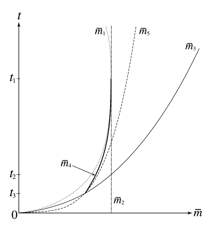
Figure 1: Various critical scales $\bar{m}_{i}$ $(i=1,\cdots,5)$ are drawn for the $SU(N)$ gauge-Higgs model with the fundamental fermion and Higgs fields for $N=$ odd, where $t_{1}=\frac{48\pi^{2}(N-1)^{3}}{N(N^{2}-3)}$, $t_{2}=\frac{24\pi^{2}(N-1)^{3}}{N^{2}(2N-3)}$ and $t_{3}=\frac{24\pi^{2}(N-1)^{3}(N^{2}-N-1)}{N^{3}(2N-3)^{2}}$.

Now, we are ready to determine the phase structure of the model. As shown in Fig.1, the lines $\bar{m}_{i}(i=1,2,3)$ divide the $\bar{m}$-$t$ plane into the several regions. Some region allows only one phase, which is nothing but the vacuum configuration. There are, however, overlapping regions in which two of the three phases remain as candidates of the vacuum configuration. In this case, one has to determine which phase gives the lowest energy among them. Fig.1 will help us understand the phase structure of the model.

Since $\bar{m}_{1}=\bar{m}_{2}$ at $t=t_{1}\equiv 48\pi^{2}\frac{(N-1)^{3}}{N(N^{2}-3)}$ and $\bar{m}_{2}=\bar{m}_{3}$ at $t=t_{2}\equiv 24\pi^{2}\frac{(N-1)^{3}}{N^{2}(2N-3)}$ (no other intersections of the curves $\bar{m}_{i}$ for $t>0$), it is convenient to consider separately the three parameter regions of $t$:

$$48\pi^{2}{{(N-1)^{3}}\over{N(N^{2}-3)}}< t, \hskip 110.96556pt(\bar{m}_{2}<\bar{m}_{3}),$$ (29)

$$24\pi^{2}{{(N-1)^{3}}\over{N^{2}(2N-3)}}< t \leq 48\pi^{2}{{(N-1)^{3}}\over{N(N^{2}-3)}},~{}~{}~{}(\bar{m}_{1}\leq\bar{m}_{2}<\bar{m}_{3}),$$ (30)

$$t \leq 24\pi^{2}{{(N-1)^{3}}\over{N^{2}(2N-3)}},~{}~{}(\bar{m}_{1}<\bar{m}_{3}\leq\bar{m}_{2}).$$ (31)

Here, the relative magnitude of $\bar{m}_{i}$ for each parameter region of $t$ is shown in the parenthesis.

(i)  $t>48\pi^{2}{{(N-1)^{3}}\over{N(N^{2}-3)}}$

We immediately observe that the scale $\bar{m}_{2}$ $(\bar{m}_{3})$ is the phase boundary between the Hosotani phase and the coexisting one (the coexisting phase and the Higgs one). There is no overlapping region of the phases for this parameter region of $t$. Thus, the vacuum configuration is given by

$$\mbox{vacuum configuration}=\left\{\begin{array}[]{lll}\mbox{Hosotani phase}&\mbox{for}&\bar{m}<\bar{m}_{2},\\ \mbox{coexisting phase}&\mbox{for}&\bar{m}_{2}<\bar{m}<\bar{m}_{3},\\ \mbox{Higgs phase}&\mbox{for}&\bar{m}_{3}<\bar{m}.\end{array}\right.$$ (32)

The order parameters in the Hosotani and coexisting phases (the coexisting and Higgs phases) are connected continuously at the phase boundary $\bar{m}_{2}$ $(\bar{m}_{3})$, so that the phase transition is the second order.

(ii)  $24\pi^{2}{{(N-1)^{3}}\over{N^{2}(2N-3)}}<t\leq 48\pi^{2}{{(N-1)^{3}}\over{N(N^{2}-3)}}$

For this parameter region of $t$, the Hosotani and coexisting phases overlap between $\bar{m}_{1}$ and $\bar{m}_{2}$. Let us consider the quantity $\Delta\bar{V}\equiv\bar{V}_{Hosotani}-\bar{V}_{coexisting}$, which is a monotonically increasing function with respect to $\bar{m}$,

$${{\partial\Delta\bar{V}}\over{\partial\bar{m}^{2}}}={1\over 2}\bar{v}^{2}(\bar{m})\geq 0,$$ (33)

as shown in the appendix. By denoting the scale giving $\bar{V}_{coexisting}=\bar{V}_{Hosotani}$ by $\bar{m}_{4}$, we can conclude that for $\bar{m}\leq\bar{m}_{4}$ $(\bar{m}_{4}<\bar{m}\leq\bar{m}_{3})$, the Hosotani (coexisting) phase is realized as the vacuum configuration. The Higgs phase can exist for $\bar{m}_{3}<\bar{m}$. Thus, we obtain that

$$\mbox{vacuum configuration}=\left\{\begin{array}[]{lll}\mbox{Hosotani phase}&\mbox{for}&\bar{m}<\bar{m}_{4},\\ \mbox{coexisting phase}&\mbox{for}&\bar{m}_{4}<\bar{m}<\bar{m}_{3},\\ \mbox{Higgs phase}&\mbox{for}&\bar{m}_{3}<\bar{m}.\end{array}\right.$$ (34)

The explicit form of the critical scale $\bar{m}_{4}$ is given by

$$\bar{m}_{4}=2\pi\sqrt{\frac{1}{2a}\left(b+\sqrt{b^{2}-4ac}\right)},$$ (35)

where

$$a = 48N^{4}(N^{2}-3N+3)^{2}\biggl{(}3(N-1)^{3}+2N(N^{2}-3N+3)\frac{t}{16\pi^{2}}\biggr{)},$$ (36)

$$b = 24N^{2}(N-1)^{2}\biggl{(}3(N-1)^{3}(N^{2}-N-1)(3N^{2}-5N+1)$$ (37)

$$\ \ +2N^{3}(2N-3)^{2}(N^{2}-3N+3)\frac{t}{16\pi^{2}}\biggr{)},$$

$$c = (N-1)^{3}\biggl{(}-9(N-1)^{4}(N^{2}-N-1)^{2}-6N(N-1)(N^{2}-N-1)$$ (38)

$$\ \ \times(11N^{4}-36N^{3}+33N^{2}-9)\frac{t}{16\pi^{2}}+4N^{2}(N^{2}-3)^{3}\biggl{(}\frac{t}{16\pi^{2}}\biggr{)}^{2}\biggr{)}.$$

The phase transition at $\bar{m}=\bar{m}_{3}$ is the second order, while that at $\bar{m}=\bar{m}_{4}$ is the first order because the order parameters are not connected continuously.

(iii)  $t\leq 24\pi^{2}{{(N-1)^{3}}\over{N^{2}(2N-3)}}$

Let us first compare the potential energy of the Hosotani phase with that of the Higgs phase. The scale $\bar{m}_{5}$ is the critical scale, at which $\bar{V}_{Hosotani}=\bar{V}_{Higgs}$ holds. Then, as shown in the appendix, we obtain that

$$\bar{V}_{Hosotani}<\bar{V}_{Higgs}\qquad{\rm for}\qquad\bar{m}<\bar{m}_{5},$$ (39)

$$\bar{V}_{Hosotani}>\bar{V}_{Higgs}\qquad{\rm for}\qquad\bar{m}>\bar{m}_{5},$$ (40)

where

$$\bar{m}_{5}\equiv\left({{(N-1)(N^{2}-N-1)}\over N^{3}}{\pi^{2}\over{24}}t\right)^{1\over 4}.$$ (41)

The parameter region of $t$ is further classified into two cases, depending on the relative magnitude between $\bar{m}_{5}$ and $\bar{m}_{3}$:

(iii-a)  $24\pi^{2}{{(N-1)^{3}(N^{2}-N-1)}\over{N^{3}(2N-3)^{2}}}<t\leq 24\pi^{2}{{(N-1)^{3}}\over{N^{2}(2N-3)}}$

In this case, the relative magnitude of $\bar{m}_{i}\ (i=1,\cdots,5)$ is given by $\bar{m}_{1}<\bar{m}_{4}\leq\bar{m}_{5}\leq\bar{m}_{3}<\bar{m}_{2}$ (see Fig.1). It immediately follows that the vacuum configuration is uniquely determined as

$$\mbox{vacuum configuration}=\left\{\begin{array}[]{lll}\mbox{Hosotani phase}&\mbox{for}&\bar{m}<\bar{m}_{4},\\ \mbox{coexisting phase}&\mbox{for}&\bar{m}_{4}<\bar{m}<\bar{m}_{3},\\ \mbox{Higgs phase}&\mbox{for}&\bar{m}_{3}<\bar{m}.\end{array}\right.$$ (42)

The vacuum structure is similar to the case (ii), and the phase transition at $\bar{m}=\bar{m}_{3}$ ($\bar{m}=\bar{m}_{4}$) is the second (first) order.

(iii-b)  $t\leq 24\pi^{2}{{(N-1)^{3}(N^{2}-N-1)}\over{N^{3}(2N-3)^{2}}}$

In this case, we have $\bar{m}_{1}\leq\bar{m}_{3}\leq\bar{m}_{5}<\bar{m}_{2}$ (see Fig.1). We observe that the Hosotani and coexisting phases overlap between $\bar{m}_{1}$ and $\bar{m}_{3}$. Let us recall that the difference of the potential energy between the Hosotani phase and the coexisting one, $\Delta\bar{V}$, is the monotonically increasing function with respect to $\bar{m}$, and we find that

$$\Delta\bar{V}(\bar{m}=\bar{m}_{3})={t\over{2\lambda}}\left({{2N-3}\over{24(N-1)}}\right)^{2}\left(t-24\pi^{2}{{(N-1)^{3}(N^{2}-N-1)}\over{N^{3}(2N-3)^{2}}}\right)\leq 0,$$ (43)

i.e. $\bar{V}_{Hosotani}\leq\bar{V}_{coexisting}$ for the parameter region of $t$ under consideration. This implies that there is no coexisting phase for this parameter region of $t$. Thus, taking Eq.(40) into account, we obtain that

$$\mbox{vacuum configuration}=\left\{\begin{array}[]{lll}\mbox{Hosotani phase}&\mbox{for}&\bar{m}<\bar{m}_{5},\\ \mbox{Higgs phase}&\mbox{for}&\bar{m}>\bar{m}_{5}.\end{array}\right.$$ (44)

The order parameters are not connected continuously at $\bar{m}_{5}$. The phase transition between the two phases is the first order and there is no coexisting phase for this parameter region of $t$.

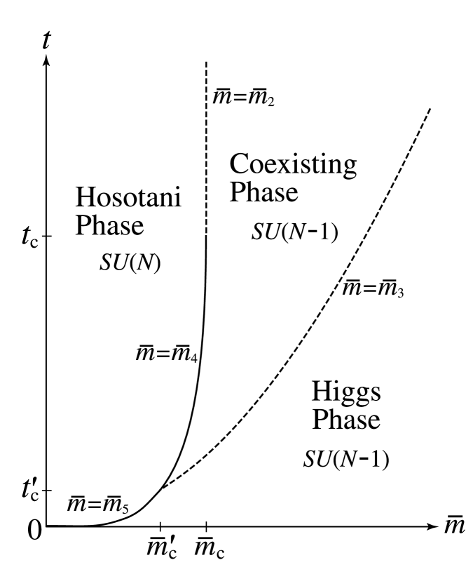
Figure 2: Phase diagram of the $SU(N)$ gauge-Higgs model with the fundamental fermion and Higgs fields for $N=$ odd, where $t_{c}=\frac{48\pi^{2}(N-1)^{3}}{N(N^{2}-3)}$, $t_{c}^{\prime}=\frac{24\pi^{2}(N-1)^{3}(N^{2}-N-1)}{N^{3}(2N-3)^{2}}$, $\bar{m}_{c}=\frac{\pi(N-1)}{N}$ and $\bar{m}_{c}^{\prime}=\frac{\pi(N-1)}{N}\sqrt{\frac{N^{2}-N-1}{N(2N-3)}}$. The solid and dashed curves denote the first- and second-order phase transitions, respectively. In each phase, the residual gauge symmetry is shown.

Collecting all the results obtained above, we depict the phase structure of the model in Fig.2. It should be noted that the Hosotani mechanism, which is usually known to break down gauge symmetry, provides a mechanism of the restoration of the gauge symmetry in the model.

2.2 $N=$ even $\geq 4$

Let us study the case $N=$ even $(\geq 4)$. The type I solution corresponding to the Hosotani phase is given by solving Eq.(11). We obtain, as shown in the appendix, that

$${\rm type~{}~{}I}~{}~{}\cdots~{}~{}\left\{\begin{array}[]{l}gL\langle A_{y}\rangle={\rm diag}\left(\pi,\pi,\cdots,\pi,-(N-1)\pi\right),\\[8.5359pt] \langle\Phi\rangle={1\over\sqrt{2}}(0,0,\cdots,0)^{T},\end{array}\right.$$ (45)

where the phase is stable for the region given by

$$0<\bar{m}<\pi.$$ (46)

The Wilson line for the configuration (45) is $-{\bf 1}_{N\times N}$ and commutes with all the generators of $SU(N)$, so that the $SU(N)$ symmetry is not broken in the phase.

In order to investigate other phases, one has to solve the third order equation with respect to $\theta_{1}$,

$$\left(1+{{t\alpha}\over{24\pi^{2}}}\right)\theta_{1}^{3}-\left({{t\alpha}\over{8\pi}}+6\pi\right)\theta_{1}^{2}+\left({{t\beta}\over{24}}-\bar{m}^{2}+12\pi^{2}\right)\theta_{1}+{{t\gamma}\over{24}}\pi+2\pi\bar{m}^{2}-8\pi^{3}=0,$$ (47)

where $\alpha,\beta$ and $\gamma$ are constants and any solution to Eq.(47) has to lie in the range

$$\pi\leq\theta_{1}\leq 2\pi,$$ (48)

as shown in the appendix. This equation has the very different structure from that for $N=$ odd (See Eq.(87) in the appendix). It does not have the solution of $\theta_{1}=2\pi$ for any values of $t$ and $\bar{m}$. This implies that the Higgs phase

$${\rm type~{}~{}II}~{}~{}\cdots~{}~{}\left\{\begin{array}[]{l}gL\langle A_{y}\rangle={\rm diag}\left(0,{{N-2}\over{N-1}}\pi,\cdots,{{N-2}\over{N-1}}\pi,-{{(N-2)^{2}}\over{N-1}}\pi\right),\\[8.5359pt] \langle\Phi\rangle={1\over\sqrt{2}}(\sqrt{2\over\lambda}m,0,\cdots,0)^{T},\end{array}\right.$$ (49)

does not exist unlike the case $N=$ odd. The Higgs phase can be realized only in the limit $L\rightarrow\infty$ (or $\bar{m}\rightarrow\infty$), as we will see later. The $SU(N)$ gauge symmetry is broken to $SU(N-1)\times U(1)$ by the Wilson line and the Higgs VEV breaks the $U(1)$, so that the residual gauge symmetry is $SU(N-1)$ for the configuration (49).

In order to see that the vacuum configuration is expected to approach the Higgs phase in the limit $\bar{m}\rightarrow\infty$, let us first note that the classical Higgs potential dominates the effective potential in the limit. Then, we obtain the nonvanishing Higgs VEV $v=\sqrt{2m/\lambda}$. It follows that the equation (6) results in $\hat{\theta}_{1}=0$ or $\theta_{1}=0$ mod $2\pi$. This result is also derived from Eq.(47) by taking the limit $\bar{m}\rightarrow\infty$. For these values of the order parameters, the equation we have to solve becomes the same equation as the one that produces the Hosotani phase for the case $N=$ odd, but in the present case, $N$ is replaced by $N-1$ ($=$ odd) with the nonvanishing $\bar{v}$. Hence, we finally arrive at the solution (49).

Our task is now to solve the equation (47) for finite sizes of $S^{1}$ and to confirm the phase structure for the case $N=$ even depicted in the Fig.3. The coexisting phase is given by

$${\rm type~{}~{}III}~{}~{}\cdots~{}~{}\left\{\begin{array}[]{l}gL\langle A_{y}\rangle={\rm diag}\left(\theta_{c},{N\over{N-1}}\pi-{\theta_{c}\over{N-1}},\cdots,{N\over{N-1}}\pi-{\theta_{c}\over{N-1}},{{-\theta_{c}}\over{N-1}}-{{N(N-2)}\over{N-1}}\pi\right),\\[8.5359pt] \langle\Phi\rangle={1\over\sqrt{2}}(\sqrt{2\over\lambda}v,0,\cdots,0)^{T},\end{array}\right.$$ (50)

where $\bar{v}=\sqrt{{2\over\lambda}(\bar{m}^{2}-(2\pi-\theta_{c})^{2})}$ and $\theta_{c}$ is the solution for the coexisting phase (see below). The $SU(N)$ gauge symmetry is broken to $SU(N-1)\times U(1)$ by the Wilson line and the Higgs VEV breaks the $U(1)$, so that the residual gauge symmetry is $SU(N-1)$ for the vacuum configuration (50).

In order to confirm that the phase structure is actually given by the Fig.3, it is convenient to consider intersections of two functions defined by

$$F(\theta_{1}) \equiv 2(\bar{m}^{2}-(2\pi-\theta_{1})^{2})(2\pi-\theta_{1}),$$ (51)

$$G(\theta_{1}) \equiv {{-t}\over{12\pi^{2}}}\left(\alpha\theta_{1}^{3}-3\pi\alpha\theta_{1}^{2}+\beta\pi^{2}\theta_{1}+\gamma\pi^{3}\right).$$ (52)

Let us note that $F(\theta_{1})=G(\theta_{1})$, in fact, reproduces Eq.(47) and $G(\theta_{1})$ is dependent of $\bar{m}$. Since the intersections of the functions $F(\theta_{1})$ and $G(\theta_{1})$ have different behavior for $t>48\pi^{2}(N-1)/N$ and $t<48\pi^{2}(N-1)/N$, as discussed in the appendix, it is convenient to investigate separately the phase structure for each region of $t$ (see Figs.4 and 5).

(i)  $t>48\pi^{2}{{N-1}\over N}$

In this parameterization of $t$, there is one solution denoted by $\theta_{c}$ for $\bar{m}>\pi$, as shown in Fig.4. The solution satisfies the condition (48) and is found to be stable, as discussed in the appendix. Since the Hosotani phase is unstable for $\bar{m}>\pi$, the coexisting phase must be the vacuum configuration for $\bar{m}>\pi$.

When the scale $\bar{m}$ approaches $\pi$, $\theta_{c}$ becomes closer to $\pi$ and is finally identical to $\pi$ at $\bar{m}=\pi$. This implies that the type III solution (coexisting phase) becomes identical to the type I solution (Hosotani phase). As the scale becomes smaller than $\pi$, the solution is outside of the required region (48). Hence, there is no coexisting phase for $\bar{m}<\pi$, so that the Hosotani phase must be the vacuum configuration for $\bar{m}<\pi$. Thus, we obtain that

$$\mbox{vacuum configuration}=\left\{\begin{array}[]{lll}\mbox{Hosotani phase}&\mbox{for}&\bar{m}<\pi,\\ \mbox{coexisting phase}&\mbox{for}&\bar{m}>\pi.\end{array}\right.$$ (53)

Since the order parameters are connected continuously at the phase boundary $\bar{m}=\pi$, the phase transition is the second order.

(ii)  $t<48\pi^{2}{{N-1}\over N}$

In this parameter region of $t$, we observe in Fig.5 that there is one solution denoted by $\theta_{c}$ for $\bar{m}>\pi$. The solution satisfies the condition (48) and is stable, so that the coexisting phase is the vacuum configuration for $\bar{m}>\pi$, as in the case (i).

Unlike the case (i), $\theta_{c}$ does not approach $\pi$ as $\bar{m}\rightarrow\pi$. When the scale $\bar{m}$ is equal to $\pi$, there appears a new solution denoted by $\theta_{c}^{\prime}=\pi$, while the $\theta_{c}$ still lies between $\pi$ and $2\pi$, as shown in Fig.5. If we go to smaller scales than $\pi$, there are two solutions $\theta_{c}^{\prime}$ and $\theta_{c}$ with $\pi<\theta_{c}^{\prime}\leq\theta_{c}<2\pi$ for $\bar{m}_{1}^{\prime}\leq\bar{m}<\pi$, where the two solutions coincide at $\bar{m}=\bar{m}_{1}^{\prime}$ (see Fig.5). Since there are no solutions in the required region of $\theta_{1}$ below the scale $\bar{m}_{1}^{\prime}$, the coexisting phase disappears and the Hosotani phase must be the vacuum configuration for $\bar{m}<\bar{m}_{1}^{\prime}$.

One has to take care about what is happening in the region of $\bar{m}_{1}^{\prime}\leq\bar{m}\leq\pi$. For this region, there are two solutions, $\theta_{c}$ and $\theta_{c}^{\prime}$, to Eq.(47) or the equation $F(\theta_{1})=G(\theta_{1})$. It turns out that the solution $\theta_{c}$ is stable but the other one is unstable, as shown in the appendix. Thus, there are two candidates for the vacuum configuration, i.e. the Hosotani phase and the coexisting phase given by $\theta_{c}$. Since $\theta_{c}^{\prime}=\theta_{c}$ ($\theta_{c}^{\prime}=\pi$) at $\bar{m}=\bar{m}_{1}^{\prime}$ ($\bar{m}=\pi$), we find that the unstable solution $\theta_{c}^{\prime}$ becomes identical to the coexisting phase given by $\theta_{c}$ (the Hosotani phase) at $\bar{m}=\bar{m}_{1}^{\prime}$ ($\bar{m}=\pi)$. This shows that the coexisting phase (the Hosotani phase) is not the vacuum configuration at the boundary $\bar{m}=\bar{m}_{1}^{\prime}$ $(\bar{m}=\pi)$. This observation implies that there exists a critical scale $\bar{m}_{4}^{\prime}$ such that

$$\bar{V}(\theta_{i},\bar{v},\bar{m}_{4}^{\prime})\bigg{|}_{\rm type~{}I}=\bar{V}(\theta_{i},\bar{v},\bar{m}_{4}^{\prime})\bigg{|}_{\rm type~{}III(\theta_{c})},$$ (54)

at which the first-order phase transition must occur. Since the above equation is satisfied only once for $\bar{m}_{1}^{\prime}\leq\bar{m}\leq\pi$, we obtain the phase structure for $t<48\pi^{2}\frac{N-1}{N}$ as

$$\mbox{vacuum configuration}=\left\{\begin{array}[]{lll}\mbox{Hosotani phase}&\mbox{for}&\bar{m}<\bar{m}_{4}^{\prime},\\ \mbox{coexisting phase}&\mbox{for}&\bar{m}>\bar{m}_{4}^{\prime}.\end{array}\right.$$ (55)

Collecting all the discussions we have made in this subsection, we confirm the phase structure depicted in Fig.3. We should emphasize again that the Hosotani mechanism works as the restoration of the gauge symmetry, as in the case $N=$ odd.

3 Other Models

In this section we study how phase structures change if we consider different representations of matter fields under the gauge group. Let us first introduce $N_{F}$ fermions in the adjoint representation under $SU(N)$ instead of those in the fundamental representation. Then, the last term in Eq.(4), which stands for the fermion one-loop correction, is replaced by

$${A\over{\pi^{2}L^{4}}}\sum_{n=1}^{\infty}\sum_{i,j=1}^{N}{1\over n^{4}}\cos(n(\theta_{i}-\theta_{j})).$$ (56)

It has been known that the function (56) is minimized by the configuration that breaks the $SU(N)$ gauge symmetry to $U(1)^{N-1}$ [19],

$$gL\langle A_{y}\rangle={\rm diag}\left({{N-1}\over N}\pi,{{N-3}\over N}\pi,\cdots,-{{N-3}\over N}\pi,-{{N-1}\over N}\pi\right).$$ (57)

Note that a zero eigenvalue located at the ${{N+1}\over 2}$th component appears for the case $N=$ odd, while all the components are nonzero for $N=$ even. This implies, again, that the phase structure is different, depending on whether $N=$ odd or even.

If $N=$ odd, it is possible for the Higgs VEV to take nonzero values, keeping the cross term vanishing and the Higgs potential minimizing, thanks to the zero in Eq.(57). Then, one of the $U(1)$’s is broken by the Higgs VEV, so that the residual gauge symmetry is $U(1)^{N-2}$. It is important to note that in the model there is only one phase whose structure does not depend on the size of the extra dimension. This is a new feature that has not been observed in the phase structures obtained in the previous section. If $N=$ even $(\geq 4)$, there appears no zero component in Eq.(57). One needs to study the effective potential carefully in order to determine the vacuum structure of the model. In case of the $SU(2)$ gauge group with $N_{F}$ massless adjoint fermions, we can perform fully analytic calculations, and the phase structure is found to be very similar to the one obtained in the previous paper, though the residual gauge symmetry in the Hosotani phase is given by $U(1)$ in this case.

Let us next consider the adjoint Higgs instead of the fundamental Higgs. Both $\langle A_{y}\rangle$ and $\langle\Phi\rangle$ belong to the adjoint representation under the $SU(N)$ gauge group. The cross term corresponding to the third term in the effective potential (4) is replaced by

$$g^{2}{\rm tr}\left([\langle A_{y}\rangle,~{}\langle\Phi\rangle]^{2}\right),$$ (58)

which is positive semidefinite. The diagonal form of $\langle\Phi\rangle$ makes the term vanish to minimize the effective potential. Then, the effective potential is divided into two parts written in terms of $\theta_{i}$ or $v$ alone. As a result, the minimization can be carried out separately with respect to the order parameters, so that the phase structure does not depend on the size of $S^{1}$. The residual gauge symmetry is determined by the generators of $SU(N)$ which commute with both $\langle A_{y}\rangle$ and $\langle\Phi\rangle$. Though we have already known that the gauge symmetry is (un)broken to $(SU(N))$ $U(1)^{N-1}$ through the Hosotani mechanism if the fermions belong to the (fundamental) adjoint representation under $SU(N)$, the actual residual gauge symmetry depends on the structure of the Higgs potential.

If we assume the same type of the Higgs potential as Eq.(2), for example, there are generally flat directions parametrized like $\bar{v}_{1}^{2}+\cdots+\bar{v}_{N-1}^{2}+(\bar{v}_{1}+\cdots+\bar{v}_{N-1})^{2}=\bar{m}^{2}/\lambda$ in the effective potential. The residual gauge symmetry is not uniquely determined in this case. For the fermions belonging to the fundamental representation under $SU(N)$, depending on the form of the Higgs VEV, the $SU(N)$ gauge symmetry is broken to its subgroup. On the other hand, for the fermions in the adjoint representation, the residual gauge symmetry is $U(1)^{N-1}$, irrespective of the flat directions.

4 Conclusions and Discussions

We have study the phase structure of the $SU(N)$ gauge-Higgs models with $N_{F}$ massless fermions on the space-time $M^{3}\otimes S^{1}$. There are two kinds of the order parameters for gauge symmetry breaking in the models. One is the vacuum expectation value of the Higgs field $\langle\Phi\rangle$ (the Higgs mechanism) and the other is the vacuum expectation value of the component gauge field for the $S^{1}$ direction $\langle A_{y}\rangle$ (the Hosotani mechanism). The former works at the tree level, while the latter is effective at the quantum level and sensitive to the size of $S^{1}$. There is also the interaction between $\langle A_{y}\rangle$ and $\langle\Phi\rangle$, which depends on the size as well. Thus, the dominant contribution to the effective potential comes from the different physical origins, depending on the size of the extra dimension. Therefore, the phase structure depends on the size (in addition to the parameters of the models) in general. This is expected to be a general feature in gauge-Higgs models on the space-time.

We have computed the effective potential for the two kinds of the order parameters in a one-loop approximation. In the calculation we have assumed that the number of the massless fermions is large enough, so that we have neglected the one-loop contributions from the gauge and Higgs fields to the effective potential. Then, we have obtained the effective potential given by Eq.(4). It turns out that the existence of the cross term in the potential, which comes from the interaction between $\langle A_{y}\rangle$ and $\langle\Phi\rangle$ in $D_{y}\Phi$, plays a crucial role to determine the phase structure of the model.

We have first considered the case that both the fermion and Higgs fields belong to the fundamental representation under $SU(N)$. The model possesses three phases called Hosotani, Higgs and coexisting phases for $N=$ odd, while for $N=$ even the model has only two phases, Hosotani and coexisting phases. The Higgs phase does not exist for finite sizes of $S^{1}$ and $N=$ even. The phase structure depends on both the size of the extra dimension and the parameter of the model. We have obtained the phase structure depicted in Fig. 2 (3) for $N=$ odd (even). It should be noted that, contrary to the usual case, the Hosotani mechanism can play a role of the restoration of gauge symmetry in the model.

We have next considered the case that the representation of the fermions is changed into the adjoint representation under $SU(N)$. The $SU(N)$ gauge symmetry is maximally broken to $U(1)^{N-1}$ through the Hosotani mechanism. If $N=$ odd, the Higgs field can acquire the nonvanishing vacuum expectation value, keeping the cross term vanishing. Then, one of the $U(1)$’s is further broken by the Higgs VEV, so that the residual gauge symmetry is $U(1)^{N-2}$. There is only one phase in the model, which does not depend on the size of the extra dimension. On the other hand, if $N=$ even $(\geq 4)$, due to the nonexistence of the zero component in the $\langle A_{y}\rangle$ unlike the case $N=$ odd, one has to study the effective potential carefully in order to investigate the phase structure of the model. The phase structure for $SU(2)$, however, can be fully studied analytically and is similar to the one obtained in the previous paper [16]. The residual gauge symmetry in the Hosotani phase is given by $U(1)$ in this case.

We have also considered the case that the Higgs field belongs to the adjoint representation under $SU(N)$. Both $\langle A_{y}\rangle$ and $\langle\Phi\rangle$ belong to the adjoint representation, and they cannot be diagonalized simultaneously, in general. The cross term, however, requires the diagonal form of $\langle\Phi\rangle$ in order for the effective potential to be minimized. Then, the effective potential is separated into two parts with respect to the order parameters in our approximation, and the minimization of the potential is carried out separately. This implies that the phase structure of the model does not depend on the size of the extra dimension and there is only one phase in the model. The residual gauge symmetry in the phase is generated by the generators of $SU(N)$ commuting with both $\langle A_{y}\rangle$ and $\langle\Phi\rangle$, and it depends on the detailed structure of the Higgs potential.

Our models have been studied on the space-time $M^{3}\otimes S^{1}$. One may wonder what will happen if we consider models on $M^{4}\otimes S^{1}$, or more generally, $M^{D-1}\otimes S^{1}$. Qualitative features such as the existence of the several phases and their structures with respect to the scale will not change even if we go to the higher dimensions. The phase structure comes from the fact that each term in the effective potential (4) has the different dependence on the size of the extra dimension. In other words, each term has its own physical origin, which is different each other and exists even in the higher dimensions. If we start with the space-time $M^{D-1}\otimes S^{1}$, the fermion one-loop correction is given by

$${{2^{[{D\over 2}]}N_{F}\Gamma(\frac{D}{2})}\over{\pi^{{D\over 2}}L^{D}}}\sum_{i=1}^{N}\sum_{n=1}^{\infty}{1\over n^{D}}\cos(n\theta_{i}).$$ (59)

The scale of the term is governed by the factor $1/L^{D}$ in place of $1/L^{4}$ in $D$ dimensions. The minimum of this function is given by the same configuration as Eqs.(16) or (45) in Sec. 2. This means that the global minimum for the correction does not depend on the total dimension. This is because the Hosotani mechanism is controlled by the infrared physics like the Casimir effect. In fact, the one-loop potential is governed only by the light modes in the Kaluza-Klein ones, so that they mainly contribute to determine the dynamics. On the contrary, the heavy modes suppresses the effective potential more as the dimension becomes higher. The cross term, which is crucial for the phase structure, also exists even in the higher dimensions as the same way. Therefore, we expect that the qualitative features found in this paper do not change even if we start with the higher dimensions.

In computing the effective potential, we have neglected the one-loop corrections to $\langle A_{y}\rangle$ from the gauge and Higgs fields. We have assumed that the number of massless fermions is large enough, so that these contributions are suppressed. One needs to take account of these contributions to the effective potential for small $N_{F}$ in order to understand the whole vacuum structure of the model. Namely, it is expected that the phase structure for small radius of $S^{1}$ is more involved because the ignored terms start to come into play in the effective potential.

We have also ignored the one-loop corrections to the Higgs potential from the gauge and Higgs fields, such as $c\frac{g^{2}}{L^{2}}\Phi^{\dagger}\Phi$ and $c^{\prime}\frac{\lambda}{L^{2}}\Phi^{\dagger}\Phi$, by assuming that the couplings $g$ and $\lambda$ are sufficiently small. Those mass corrections are irrelevant to the model considered in Sec.2, but they could cause gauge symmetry restoration at very small scales for models with nonvanishing Higgs VEV, like the models with one phase found in Sec.3. Mass corrections to Higgs potentials at finite temperatures or finite scales of extra dimensions have been investigated in many literature [3, 17, 18] and their effects on gauge symmetry breaking/restoration are well understood. Since the subject is not our main concerns, we will not discuss it any more.

There are several directions to extend our studies. It is interesting to investigate how gauge symmetry breaking patterns can be rich in the phase diagram by introducing matter fields belonging to various representations of gauge groups. This study has the relation with the new approach to the gauge hierarchy problem we proposed in the previous paper. We have considered the massless fermions through the analyses. In connection with the suppression of the effective potential by the large fermion number, a massive fermion also modifies the size of the fermion one-loop correction like ${\rm e}^{-mL}/L^{4}$ for $L>m^{-1}$. It is interesting to see how massive fermions affect the phase structure. We should finally stress that if the Standard Model were embedded in a higher dimensional theory with a multiply connected space, our studies would have physical importance because the theory is just in a class of the gauge-Higgs system on multiply connected spaces. It would be of importance to investigate the phase structure and clarify its physical consequences at low energies. Those will be reported elsewhere.

Acknowledgements

K.T would like to thank the Dublin Institute for Advanced Study for warm hospitality, where part of this work was done. This work was supported in part by a JSPS Research Fellowship for Young Scientists (H.H).

Appendix

(A)  Parametrization of the vacuum expectation value for the Higgs field

We shall show that the parameterization (3) of the vacuum expectation value for the Higgs field can minimize the effective potential (4).

The classical part of the effective potential for $\langle A_{y}\rangle$ and $\langle\Phi\rangle$ with every position being filled is given by

$$V_{cl} = -{1\over 2}m^{2}\sum_{i=1}^{N}|v_{i}|^{2}+{\lambda\over 8}\left(\sum_{i=1}^{N}|v_{i}|^{2}\right)^{2}+\frac{1}{2L^{2}}\sum_{i=1}^{N}\hat{\theta}_{i}^{2}|v_{i}|^{2},$$ (60)

where $\hat{\theta}_{i}=\theta_{i}$ mod $2\pi$ with $|\hat{\theta}_{i}|\leq\pi$ for $i=1,\cdots,N$. Without loss of generality, we can assume that ${\left|{\hat{\theta}_{1}}\right|}\leq{\left|{\hat{\theta}_{2}}\right|}\leq\cdots\leq{\left|{\hat{\theta}_{N}}\right|}$. Then, it is convenient to rewrite $V_{cl}$ into the form

$$V_{cl} = V_{1}+V_{2},$$ (61)

where

$$V_{1} = -\frac{1}{2L^{2}}(m^{2}L^{2}-\hat{\theta}_{1}^{2})\sum_{i=1}^{N}|v_{i}|^{2}+{\lambda\over 8}\left(\sum_{i=1}^{N}|v_{i}|^{2}\right)^{2},$$ (62)

$$V_{2} = \frac{1}{2L^{2}}\sum_{i=2}^{N}(\hat{\theta}_{i}^{2}-\hat{\theta}_{1}^{2})|v_{i}|^{2}.$$ (63)

Note that $V_{1}$ depends only on $\sum_{i=1}^{N}|v_{i}|^{2}$ (and $\hat{\theta}_{i}$) and $V_{2}$ is positive semidefinite.

Let us now consider a minimization problem of $V_{cl}$ for fixed $\theta_{i}$ ($i=1,\cdots,N$). Suppose that the minimum of $V_{1}$ for fixed $\theta_{i}$ is realized by $\sum_{i=1}^{N}|v_{i}|^{2}=v^{2}$ for a real constant $v$. Then, it is easy to see that the configuration $\langle\Phi\rangle=\frac{1}{\sqrt{2}}(v_{1},0,\cdots,0)^{T}$ with $|v_{1}|^{2}=v^{2}$ gives the minimum of $V_{cl}$ for fixed $\theta_{i}$, because the configuration realizes the minimum values of $V_{1}$ and $V_{2}$ simultaneously, so that it must be a configuration which minimizes $V_{cl}$. By using a $U(1)$ symmetry to make $v_{1}$ real, we arrive at the expression (3). Since the incorporation of quantum corrections to $\langle A_{y}\rangle$ does not alter the above discussion, we have proved the parameterization (3) in the text.

(B)  Expressions and results

We shall derive some expressions and results used in the text.

(B)-1  Hosotani phase and its stability

The Hosotani phase is obtained by solving the equation (11) and the Higgs VEV is given by Eq.(10) in the text. We work on the space-time $M^{3}\otimes S^{1}$, so that there is a formula,

$$\sum_{n=1}^{\infty}{1\over n^{4}}\cos(nx)={{-1}\over{48}}x^{2}(x-2\pi)^{2}+{{\pi^{4}}\over{90}}\qquad\mbox{for}\ 0\leq x\leq 2\pi$$ (64)

from which we have

$$\sum_{n=1}^{\infty}{1\over n^{3}}\sin(nx) = {1\over{12}}x(x-\pi)(x-2\pi),$$ (65)

$$\sum_{n=1}^{\infty}{1\over{n^{2}}}\cos(nx) = {1\over 4}x(x-2\pi)+{\pi^{2}\over 6}.$$ (66)

Note that the minimum of the function (64) is located at $x=\pi$.

To make our analysis simple, let us assume that $\theta_{i}(i=1,\cdots,N-1)$ lies in the range of $0\leq\theta_{i}<2\pi$. This can be done without loss of generality. Applying the formula (65) to Eq.(11), we obtain

$$\biggl{(}\theta_{k}+\sum_{i=1}^{N-1}\theta_{i}-2\pi q\biggr{)}\biggl{(}\theta_{k}^{2}+\Bigl{(}\sum_{i=1}^{N-1}\theta_{i}-2\pi(q-1)\Bigr{)}^{2}-\theta_{k}\Bigl{(}\sum_{i=1}^{N-1}\theta_{i}-2\pi(q-1)\Bigr{)}$$

$$\qquad-\pi\theta_{k}-\pi\Bigl{(}\sum_{i=1}^{N-1}\theta_{i}-2\pi(q-1)\Bigr{)}\biggr{)}=0\qquad\mbox{for}\ k=1,2,\cdots,N-1,$$ (67)

where the integer $q$ is defined by the requirement

$$0\leq\sum_{i=1}^{N-1}\theta_{i}-2\pi(q-1)<2\pi.$$ (68)

Let us first study the case given by

$$\theta_{k}+\sum_{i=1}^{N-1}\theta_{i}=2\pi q\qquad\mbox{for}\ k=1,2,\cdots,N-1.$$ (69)

The solution to the equation is obtained as

$$\theta\equiv\theta_{k}=\frac{2\pi q}{N}\ \ (k=1,\cdots,N-1),\quad q=0,1,\cdots,N-1.$$ (70)

Knowing that the effective potential is, now, recast in

$$\bar{V}={{AN}\over{\pi^{2}}}\sum_{n=1}^{\infty}{1\over n^{4}}\cos(n{{2\pi q}\over{N}}),$$ (71)

we find that the potential is minimized at $q=\frac{N-1}{2}$ for $N=$ odd and at $q=\frac{N}{2}$ for $N=$ even. Thus, we have

$$(\bar{v},\theta)=\left\{\begin{array}[]{ll}(0,~{}~{}{{N-1}\over N}\pi),&N={\rm odd},\\[11.38092pt] (0,~{}~{}\pi),&N={\rm even},\end{array}\right.$$ (72)

which give the solutions (16) and (45) corresponding to the Hosotani phase in the text.

Let us next discuss the stability of the above solution against small fluctuations. The stability is guaranteed if all the eigenvalues of the Hessian is positive definite. The Hessian is given by the second derivative of the effective potential with respect to the order parameters,

$$H\equiv\left(\begin{array}[]{cccc}{{\partial^{2}\bar{V}}\over{\partial\bar{v}^{2}}}&{{\partial^{2}\bar{V}}\over{\partial\bar{v}\partial\theta_{1}}}&\cdots&{{\partial^{2}\bar{V}}\over{\partial\bar{v}\partial\theta_{N-1}}}\\ {{\partial^{2}\bar{V}}\over{\partial\bar{v}\partial\theta_{1}}}&{{\partial^{2}\bar{V}}\over{\partial\theta_{1}^{2}}}&\cdots&{{\partial^{2}\bar{V}}\over{\partial\theta_{1}\partial\theta_{N-1}}}\\ \vdots&\vdots&\ddots&\vdots\\ {{\partial^{2}\bar{V}}\over{\partial\bar{v}\partial\theta_{N-1}}}&{{\partial^{2}\bar{V}}\over{\partial\theta_{1}\partial\theta_{N-1}}}&\cdots&{{\partial^{2}\bar{V}}\over{\partial\theta^{2}_{N-1}}}\end{array}\right).$$ (73)

The matrix $H$ evaluated at the solution becomes

$$H=\left(\begin{array}[]{ccccc}F&0&\cdots&\cdots&0\\ 0&2C&C&\cdots&C\\ \vdots&C&\ddots&&C\\ \vdots&\vdots&&\ddots&\vdots\\ 0&C&\cdots&\cdots&2C\\ \end{array}\right),$$ (74)

where we have defined

$$F\equiv-\bar{m}^{2}+\left({{2\pi q}\over{N}}\right)^{2},~{}~{}C\equiv{A\over\pi^{2}}\sum_{n=1}^{\infty}{{-1}\over n^{2}}\cos\left(n{{2\pi q}\over N}\right)$$ (75)

with $q={{N-1}\over 2}$ or ${N\over 2}$. The eigenvalues of the matrix $H$ are found to be $F$, $C$ ($(N-2)$ degeneracy) and $NC$, and hence all the eigenvalues of $H$ for the given values of $q$ is positive as long as $0<\bar{m}<{{2\pi q}\over N}$. This means that each solution in Eq.(72) is stable for the scale region given by

$$\begin{array}[]{lll}0<\bar{m}<{{N-1}\over N}\pi&{\rm for}&N={\rm odd},\\[8.5359pt] 0<\bar{m}<\pi&{\rm for}&N={\rm even}.\end{array}$$ (76)

We have obtained Eqs.(24) and (46) in the text.

Let us next consider the other solutions to Eq.(67),

$$\biggl{(}\theta_{k}^{2}+\Bigl{(}\sum_{i=1}^{N-1}\theta_{i}-2\pi(q-1)\Bigr{)}^{2}-\theta_{k}\Bigl{(}\sum_{i=1}^{N-1}\theta_{i}-2\pi(q-1)\Bigr{)}$$

$$\quad-\pi\theta_{k}-\pi\Bigl{(}\sum_{i=1}^{N-1}\theta_{i}-2\pi(q-1)\Bigr{)}\biggr{)}=0$$ (77)

for $k=1,\cdots,N-1$. Any solutions satisfying Eq.(77) give a negative diagonal component $\frac{\partial^{2}\bar{V}}{\partial\theta_{k}^{2}}$ in $H$. It is not difficult to show that

$${{\partial^{2}\bar{V}}\over{\partial\theta_{k}^{2}}} = {A\over\pi^{2}}\sum_{n=1}^{\infty}{{-1}\over{n^{2}}}\biggl{(}\cos(n\theta_{k})+\cos(n\sum_{i=1}^{N-1}\theta_{i})\biggr{)}$$ (78)

$$= -{{A}\over{12\pi^{2}}}\biggl{(}\theta_{k}+\sum_{i=1}^{N-1}\theta_{i}-2\pi q\biggr{)}^{2}<0,$$

where we have used the formula (66) and Eq.(77). This implies that any solutions satisfying Eq.(77) are not stable against small fluctuations, so that we exclude such solutions from our discussions hereafter.

(B)-2  Higgs and coexisting phases and their stabilities

Let us next consider the case given by Eq.(10),

$$-\bar{m}^{2}+{\lambda\over 2}\bar{v}^{2}+\hat{\theta}_{1}^{2}=0.$$ (79)

In this case, the equations we solve are given by Eqs.(12) and (13). Applying the formula (65) to Eq.(13), we obtain the same equation as Eq.(69), in which the case of $k=1$ is excluded in the present case. The equations obtained imply that

$$\theta_{2}=\theta_{3}=\cdots=\theta_{N-1}\equiv\bar{\theta}.$$ (80)

As the result, the equation (13) finally yields the relation,

$$\theta_{1}+(N-1)\bar{\theta}=2\pi l$$ (81)

for some integer $l$. Since it is enough to consider the region $0\leq\bar{\theta}\leq\pi$ and we have required the sequence ${\left|{\hat{\theta}_{1}}\right|}\leq{\left|{\hat{\theta}_{2}}\right|}\leq\cdots\leq{\left|{\hat{\theta}_{N}}\right|}$, our solutions also have to satisfy the constraint ${\left|{\hat{\theta}_{1}}\right|}\leq{\left|{\bar{\theta}}\right|}$ in addition to the relation (81). Among possible solutions satisfying those, one needs the solution that minimizes the effective potential, which is now recast in

$$\bar{V}=-{1\over 2}\bar{m}^{2}\bar{v}^{2}+{\lambda\over 8}\bar{v}^{4}+{1\over 2}\hat{\theta}_{1}^{2}\bar{v}^{2}+{A\over\pi^{2}}\sum_{n=1}^{\infty}{1\over n^{4}}\left(\cos(n\theta_{1})+(N-1)\cos(n\bar{\theta}))\right),$$ (82)

where we have used Eqs.(80) and (81). The integer $l$ must be determined in such a way that the potential energy is minimized. For general $l$, Eq.(81) and other constraints restrict allowed regions of $\theta_{1}$ and $\bar{\theta}$. It is not difficult to see that the minimum of the effective potential (82) can be realized when $l={{N-1}\over 2}$ for $N=$odd or $l={N\over 2}$ for $N=$ even and

$${{N-1}\over N}\pi\leq\bar{\theta}\leq\pi, \quad 0\leq\theta_{1}\leq{{N-1}\over N}\pi,\quad\mbox{for}\ N=\mbox{odd},$$ (83)

$${{N-2}\over{N-1}}\pi\leq\bar{\theta}\leq\pi, \quad\pi\leq\theta_{1}\leq 2\pi,\hskip 36.98866pt\mbox{for}\ N=\mbox{even}.$$ (84)

Thus, we have obtained Eqs.(26) and (48) in the text.

Now, the effective potential is rewritten, depending on whether $N$ is even or odd, in terms of $\bar{v}$ and $\theta_{1}$ alone, as

$$\bar{V}_{N=odd} = -{1\over 2}\bar{m}^{2}\bar{v}^{2}+{\lambda\over 8}\bar{v}^{4}+{1\over 2}\hat{\theta}_{1}^{2}\bar{v}^{2}$$ (85)

$$+ {A\over\pi^{2}}\sum_{n=1}^{\infty}{1\over n^{4}}\biggl{(}\cos(n\theta_{1})+(N-1)\cos\Bigl{(}n\bigl{(}\pi+{{\theta_{1}}\over{N-1}}\bigr{)}\Bigr{)}\biggr{)},$$

$$\bar{V}_{N=even} = -{1\over 2}\bar{m}^{2}\bar{v}^{2}+{\lambda\over 8}\bar{v}^{4}+{1\over 2}{\hat{\theta}}_{1}^{2}\bar{v}^{2}$$ (86)

$$+ {A\over\pi^{2}}\sum_{n=1}^{\infty}{1\over n^{4}}\biggl{(}\cos(n\theta_{1})+(N-1)\cos\Bigl{(}n\bigl{(}{{\theta_{1}}\over{N-1}}+{{N-2}\over{N-1}}\pi\bigr{)}\Bigr{)}\biggr{)}.$$

It follows from Eqs.(83) and (84) that the relation between $\hat{\theta}_{1}$ and $\theta_{1}$ is given by $\hat{\theta}_{1}=\theta_{1}$ for $N=$ odd and $\hat{\theta}_{1}=\theta_{1}-2\pi$ for $N=$ even. Our remaining task is to solve the equation (12) under the relation (81) with $q=\frac{N-1}{2}$ $(\frac{N}{2})$ for $N=$ odd (even) or, equivalently, to solve the equation from the first derivative of the potential (85) or (86) with respect to $\theta_{1}$ with Eq.(79).

(B)-3  $N=$odd

As explained above, the equation we solve becomes

$$\theta_{1}\left({2\over\lambda}(\bar{m}^{2}-\theta_{1}^{2})-{A\over{12\pi^{2}}}\Bigl{(}{{N(N^{2}-3N+3)}\over{(N-1)^{3}}}\theta_{1}^{2}-3\pi\theta_{1}+{{2N-3}\over{N-1}}\pi^{2}\Bigr{)}\right)=0,$$ (87)

which reads

$$\theta_{1}=0,$$ (89)

or

$$\left(1+{t\over{24\pi^{2}}}{{N(N^{2}-3N+3)}\over{(N-1)^{3}}}\right)\theta_{1}^{2}-{t\over{8\pi}}\theta_{1}-\bar{m}^{2}+{t\over{24}}{{2N-3}\over{N-1}}=0.$$

Here we have introduced $t\equiv\lambda A(=4\lambda N_{F})$.

Let us first study the case $\theta_{1}=0$. The relation (81) with $l={{N-1}\over 2}$ yields $\theta_{2}=\theta_{3}=\cdots=\theta_{N-1}=\pi$ and $\theta_{N}=-(N-2)\pi$. And $\bar{v}=\sqrt{2/\lambda}~{}\bar{m}$ from Eq.(79). Thus, we have obtained the type II solution corresponding to the Higgs phase (19) in the text. The stability of the type II solution is studied by the eigenvalues of the matrix $H$ evaluated at the solution. It is given by

$$H=\left(\begin{array}[]{ccccc}2\bar{m}^{2}&0&\cdots&\cdots&0\\ 0&G&B&\cdots&B\\ \vdots&B&2B&&B\\ \vdots&\vdots&&\ddots&\vdots\\ 0&B&\cdots&\cdots&2B\\ \end{array}\right),$$ (90)

where we have defined $B\equiv{A\over{12}}$ and $G\equiv{2\over\lambda}\bar{m}^{2}-B$. The eigenvalues of the matrix are found to be $2\bar{m}^{2}$, ${A\over{12}}$ ($(N-3)$ degeneracy) and $x_{\pm}$, where

$$x_{\pm}\equiv{1\over 2}\Biggl{(}G+(N-1)B\pm\sqrt{(G+(N-1)B)^{2}-4B((N-1)G-(N-2)B)}\Biggr{)}.$$ (91)

The condition that the eigenvalues $x_{\pm}$ are positive is given by

$$\bar{m}^{2}>{{2N-3}\over{N-1}}{{\lambda A}\over{24}}={{2N-3}\over{N-1}}{t\over{24}}\equiv\bar{m}_{3}^{2}.$$ (92)

Thus, we have obtained Eq.(25) in the text.

Let us next study the solutions given by Eq.(89), i.e.

$$\theta_{1}^{\pm}(\bar{m})={1\over{2(1+{{t}\over{24\pi^{2}}}C_{0})}}\left({{t\over{8\pi}}\pm{{N^{2}-3}\over{24(N-1)^{2}}}{t\over\pi}\sqrt{S(\bar{m})}}\right),$$ (93)

where

$$S(\bar{m})\equiv 1-C_{1}\left({\pi^{2}\over t}\right)+{1\over t^{2}}\left(C_{2}\pi^{2}+C_{3}t\right)\bar{m}^{2}$$ (94)

with $C_{i}(i=0,1,2,3)$ being defined by

$$C_{0} \equiv {{N(N^{2}-3N+3)}\over{(N-1)^{3}}},~{}~{}C_{1}\equiv{{96(2N-3)(N-1)^{3}}\over{(N^{2}-3)^{2}}},$$ (95)

$$C_{2} \equiv {{2304(N-1)^{4}}\over{(N^{2}-3)^{2}}},~{}~{}C_{3}\equiv{{96N(N-1)(N^{2}-3N+3)}\over{(N^{2}-3)^{2}}}.$$ (96)

Let us study the stability of the solutions. To this end, we note that the order parameters in this case are reduced to two, that is, $\bar{v}$ and $\theta_{1}$. Then, the matrix $H$ becomes the $2\times 2$ matrix,

$$H\equiv\left(\begin{array}[]{cc}{{\partial^{2}\bar{V}}\over{\partial\bar{v}^{2}}}&{{\partial^{2}\bar{V}}\over{\partial\bar{v}\partial\theta_{1}}}\\ {{\partial^{2}\bar{V}}\over{\partial\bar{v}\partial\theta_{1}}}&{{\partial^{2}\bar{V}}\over{\partial\theta_{1}^{2}}}\\ \end{array}\right),$$ (97)

where each component evaluated at the solutions is given by

$${{\partial^{2}\bar{V}}\over{\partial\bar{v}^{2}}} = \lambda\bar{v}^{2},\qquad{{\partial^{2}\bar{V}}\over{\partial\bar{v}\partial\theta_{1}}}=2\theta_{1}^{\pm}\bar{v}$$ (98)

$${{\partial^{2}\bar{V}}\over{\partial\theta_{1}^{2}}} = \bar{v}^{2}-{A\over{\pi^{2}}}\sum_{n=1}^{\infty}{1\over n^{2}}\left(\cos(n\theta_{1}^{\pm})+{1\over{N-1}}\cos(\pi+{\theta_{1}^{\pm}\over{N-1}})\right)$$ (99)

$$= {A\over{12\pi^{2}}}\left(-{{2N(N^{2}-3N+3)}\over{(N-1)^{3}}}(\theta_{1}^{\pm})^{2}+3\pi\theta_{1}^{\pm}\right),$$

where we have used the formula (66). Then, the determinant of $H$ is calculated as

$${\rm det}~{}H=\mp\bar{v}^{2}(\bar{m})\theta_{1}^{\pm}(\bar{m})\left({{t(N^{2}-3)}\over{12\pi(N-1)^{2}}}\sqrt{S(\bar{m})}\right).$$ (100)

Since $\theta_{1}$ is larger than zero, the solution $\theta_{1}^{+}$ gives a negative determinant of $H$, so that $\theta_{1}^{+}(\bar{m})$ is unstable and is excluded from our discussions. Hence, we have obtained the type III solution $\theta_{1}^{-}(\bar{m})$ with $\bar{v}=\sqrt{{2\over\lambda}(\bar{m}^{2}-(\theta_{1}^{-})^{2})}$ corresponding to the coexisting phase (22) in the text.

The solution $\theta_{1}^{-}(\bar{m})$ must satisfy the reality condition $(\theta_{1}^{-}(\bar{m}))^{*}=\theta_{1}^{-}(\bar{m})$ and $0\leq\theta_{1}^{-}(\bar{m})\leq{{N-1}\over N}\pi$, as shown in Eq.(83). The reality condition is furnished if $t\geq C_{1}\pi^{2}$ or if

$$\bar{m}\geq\left({{C_{1}\pi^{2}t-t^{2}}\over{C_{2}\pi^{2}+C_{3}t}}\right)^{{1\over 2}}\equiv\bar{m}_{1}\qquad\mbox{for}\ t<C_{1}\pi^{2}.$$ (101)

The condition $0\leq\theta_{1}^{-}(\bar{m})$ yields that

$$\bar{m}\leq\left({{2N-3}\over{N-1}}{t\over{24}}\right)^{{1\over 2}}\equiv\bar{m}_{3},$$ (102)

while the condition $\theta_{1}^{-}(\bar{m})\leq{{N-1}\over N}\pi$ requires that

$$\bar{m}\geq{{N-1}\over{N}}\pi\equiv\bar{m}_{2}\quad{\rm for}\quad t\geq 48\pi^{2}{{(N-1)^{3}}\over{N(N^{2}-3)}}.$$ (103)

The latter condition is always satisfied for $t<48\pi^{2}{{(N-1)^{3}}\over{N(N^{2}-3)}}$.

The relative magnitude in the scales $\bar{m}_{i}$ $(i=1,2,3)$ is important to understand the allowed region of the coexisting phase. It is easy to show that $\bar{m}_{1}<\bar{m}_{3}$ is always satisfied, irrespective of the values of $N$ and $t$, while the relative magnitude of $\bar{m}_{2}$ and $\bar{m}_{3}$ depends on the parameter $t$,

$$\bar{m}_{2}\leq(>)\bar{m}_{3}\quad{\rm for}\quad t\geq(<)24\pi^{2}{{(N-1)^{3}}\over{N^{2}(2N-3)}}.$$ (104)

The relation $\bar{m}_{1}\leq\bar{m}_{2}$ is always satisfied, where the equality holds for $t=48\pi^{2}{{(N-1)^{3}}\over{N(N^{2}-3)}}$. We have understood the scale relations given in the parentheses in Eqs.(29), (30) and (31). In Fig.1, the curves of the critical scales $\bar{m}_{i}$ are depicted in the $\bar{m}$-$t$ plane, and the relative magnitude of $\bar{m}_{i}$ will be understood clearly there. Noting that $C_{1}\pi^{2}>48\pi^{2}\frac{(N-1)^{3}}{N(N^{2}-3)}$ and collecting the results obtained above, we find that the allowed region of the coexisting phase is given by

$$\bar{m}_{2}\leq\bar{m}\leq\bar{m}_{3}\qquad \ t>48\pi^{2}\frac{(N-1)^{3}}{N(N^{2}-3)},$$ for (105)

$$\bar{m}_{1}\leq\bar{m}\leq\bar{m}_{3}\qquad \ t\leq 48\pi^{2}\frac{(N-1)^{3}}{N(N^{2}-3)}.$$ for (106)

It will be useful to evaluate the values of $\theta_{1}^{-}(\bar{m})$ at the boundaries in Eqs.(105) and (106). One can show that

$$\theta_{1}^{-}(\bar{m}_{2})=\frac{N-1}{N}\pi\ \ \mbox{and}\ \ \theta_{1}^{-}(\bar{m}_{3})=0\quad \ t\geq 48\pi^{2}\frac{(N-1)^{3}}{N(N^{2}-3)},$$ for (107)

$$\theta_{1}^{-}(\bar{m}_{1})=\frac{t}{16\pi\left(1+\frac{t}{24\pi^{2}}C_{0}\right)}\ \ \mbox{and}\ \ \theta_{1}^{-}(\bar{m}_{3})=0\quad \ t<48\pi^{2}\frac{(N-1)^{3}}{N(N^{2}-3)}.$$ for (108)

Let us study the behavior of the type III solution with respect to the scale $\bar{m}$. We first note that the solution $\theta_{1}^{-}(\bar{m})$ is a monotonically decreasing function of $\bar{m}$.

$${{\partial\theta_{1}^{-}(\bar{m})}\over{\partial\bar{m}^{2}}}=-{{24\pi(N-1)^{2}}\over{t(N^{2}-3)}}{1\over{\sqrt{S(\bar{m})}}}<0.$$ (109)

On the other hand, $\bar{v}^{2}(\bar{m})$ is a monotonically increasing function of $\bar{m}$

$${{\partial\bar{v}^{2}}\over{\partial\bar{m}^{2}}}={2\over\lambda}\left(1+\theta_{1}^{-}(\bar{m}){{48(N-1)^{2}}\over{(N^{2}-3)\sqrt{S(\bar{m})}}}{\pi\over t}\right)>0$$ (110)

for the region (83). Since $\bar{v}^{2}(\bar{m})$ can be written as

$$\bar{v}^{2}(\bar{m})=\frac{N(N^{2}-3N+3)t}{12\pi^{2}(N-1)^{3}\lambda}\biggl{(}\theta_{1}^{-}(\bar{m})-\frac{N-1}{N}\pi\biggr{)}\biggl{(}\theta_{1}^{-}(\bar{m})-\frac{(N-1)(2N-3)}{N^{2}-3N+3}\pi\biggr{)},$$ (111)

$\bar{v}^{2}(\bar{m})$ is positive semidefinite for $0\leq\theta_{1}^{-}(\bar{m})\leq\frac{N-1}{N}\pi$, as it should be. One can also show that

$$\bar{v}^{2}(\bar{m}_{2}) = 0\qquad\mbox{for}\ t\geq 48\pi^{2}\frac{(N-1)^{3}}{N(N^{2}-3)},$$ (112)

$$\bar{v}^{2}(\bar{m}_{3}) = \frac{2}{\lambda}\bar{m}_{3}^{2}.$$ (113)

It follows together with Eq.(107) and (108) that the coexisting phase is found to be continuously connected to the Hosotani phase (the Higgs phase) at the boundary $\bar{m}=\bar{m}_{2}$ ($\bar{m}=\bar{m}_{3}$) for $t\geq 48\pi^{2}\frac{(N-1)^{3}}{N(N^{2}-3)}$.

We have studied the allowed region of the coexisting phase with respect to the parameters $\bar{m}$ and $t$. We have obtained that (i) when $t>48\pi^{2}{{(N-1)^{3}}\over{N(N^{2}-3)}}$, the relative magnitude of the scales is given by $\bar{m}_{1}<\bar{m}_{2}<\bar{m}_{3}$, and the coexisting phase exists between $\bar{m}_{2}$ and $\bar{m}_{3}$, (ii) when $24\pi^{2}{{(N-1)^{3}}\over{N^{2}(2N-3)}}<t\leq 48\pi^{2}{{(N-1)^{3}}\over{N(N^{2}-3)}}$, the relative magnitude of the scales is given by $\bar{m}_{1}\leq\bar{m}_{2}<\bar{m}_{3}$, and the coexisting phase lies between $\bar{m}_{1}$ and $\bar{m}_{3}$, (iii) when $t\leq 24\pi^{2}{{(N-1)^{3}}\over{N^{2}(2N-3)}}$, we have $\bar{m}_{1}<\bar{m}_{3}\leq\bar{m}_{2}$, and the coexisting phase is between $\bar{m}_{1}$ and $\bar{m}_{3}$. We have arrived at the classification used in the text, Eqs.(29), (30) and (31). Fig.1 will help our understanding of the phase structure.

Let us finally calculate the potential energy for each phase.

$$\bar{V}_{Hosotani} = A\pi^{2}\left(-\frac{(N^{2}-1)^{2}}{48N^{3}}+{N\over{90}}\right),$$ (114)

$$\bar{V}_{Higgs} = -{\bar{m}^{4}\over{2\lambda}}+A\pi^{2}\left(-{{(N-1)}\over{48}}+{{N}\over{90}}\right),$$ (115)

$$\bar{V}_{coexisting} = -{{1}\over{2\lambda}}\left(\bar{m}^{2}-\theta_{1}^{-}(\bar{m})^{2}\right)^{2}+{A\over\pi^{2}}\Biggl{(}-{1\over{48}}{\theta_{1}^{-}(\bar{m})}^{2}\Bigl{(}\theta_{1}^{-}(\bar{m})-2\pi\Bigr{)}^{2}$$ (116)

$$\ \ -{{N-1}\over{48}}\Bigl{(}\pi+{{\theta_{1}^{-}(\bar{m})}\over{N-1}}\Bigr{)}^{2}\Bigl{(}{{\theta_{1}^{-}(\bar{m})}\over{N-1}}-\pi\Bigr{)}^{2}+{N\over{90}}\pi^{4}\Biggr{)},$$

where $\theta_{1}^{-}(\bar{m})$ is given by Eq.(93). It is not difficult to show that the energy difference $\Delta\bar{V}\equiv\bar{V}_{Hosotani}-\bar{V}_{coexisting}$ is a monotonically increasing function of $\bar{m}^{2}$,

$${{\partial}\over{\partial\bar{m}^{2}}}\Delta\bar{V}(\bar{m})={1\over 2}\bar{v}(\bar{m})^{2}\geq 0,$$ (117)

where we have used the equation (89). We also observe that

$$\bar{V}_{Hosotani}-\bar{V}_{Higgs} = {1\over{2\lambda}}\left(\bar{m}^{4}-{{(N-1)(N^{2}-N-1)}\over{N^{3}}}{{\pi^{2}}\over{24}}t\right)$$ (118)

$$\equiv {1\over{2\lambda}}\left(\bar{m}^{4}-(\bar{m}_{5})^{4}\right),$$

which gives the critical scale given by Eq. (41) in the text.

(B)-4  $N=$ even

Let us study the case $N=$ even. The equation we solve is given, from Eq.(86), by

$$- {2\over\lambda}\left(\bar{m}^{2}-(2\pi-\theta_{1})^{2}\right)(2\pi-\theta_{1})$$ (119)

$$+ {A\over\pi^{2}}\sum_{n=1}^{\infty}{{-1}\over n^{3}}\left(\sin(n\theta_{1})+\sin(n({\theta_{1}\over{N-1}}+{{N-2}\over{N-1}}\pi))\right)=0,$$

where we have eliminated $\bar{v}^{2}$ by $\bar{v}^{2}={2\over\lambda}(\bar{m}^{2}-(2\pi-\theta_{1})^{2})$. Using the formula (65), the above equation becomes

$$\left(1+{{t\alpha}\over{24\pi^{2}}}\right)\theta_{1}^{3}-\left({{t\alpha}\over{8\pi}}+6\pi\right)\theta_{1}^{2}+\left({{t\beta}\over{24}}-\bar{m}^{2}+12\pi^{2}\right)\theta_{1}+{{t\gamma}\over{24}}\pi+2\pi\bar{m}^{2}-8\pi^{3}=0,$$ (120)

where

$$\alpha\equiv{{N(N^{2}-3N+3)}\over{(N-1)^{3}}},~{}\beta\equiv{{N(2N^{2}-7N+8)}\over{(N-1)^{3}}},~{}\gamma\equiv{{N(N-2)}\over{(N-1)^{3}}}.$$ (121)

This is the equation (47) in the text. Instead of solving the equation (120) directly, it turns out to be convenient to study intersections of two functions $F(\theta_{1})$ and $G(\theta_{1})$ followed from Eq.(120). Here, $F(\theta_{1})$ and $G(\theta_{1})$ are

$$F(\theta_{1}) \equiv 2(\bar{m}^{2}-(2\pi-\theta_{1})^{2})(2\pi-\theta_{1}),$$ (122)

$$G(\theta_{1}) \equiv {{-t}\over{12\pi^{2}}}\left(\alpha\theta_{1}^{3}-3\pi\alpha\theta_{1}^{2}+\beta\pi^{2}\theta_{1}+\gamma\pi^{3}\right),$$ (123)

$$= {{-t\alpha}\over{12\pi^{2}}}(\theta_{1}-\pi)(\theta_{1}-\theta_{1}^{-})(\theta_{1}-\theta_{1}^{+}),$$ (124)

where

$$\theta_{1}^{\pm}=\pi\left(1\pm{{N-1}\over{\sqrt{N^{2}-3N+3}}}\right).$$ (125)

Let us note that $G(\theta_{1})$ is independent of $\bar{m}$ and that $F(\theta_{1})=G(\theta_{1})$, of course, reproduces the equation (120).

We study the behaviors of the intersections of $F(\theta_{1})=G(\theta_{1})$ with respect to the scale $\bar{m}$ and the parameter $t$. We first note that the number of the intersections of the functions $F(\theta_{1})$ and $G(\theta_{1})$ is either one or three. The Higgs VEV is also written, from Eq.(119) after using the formula (65), as

$$\bar{v}^{2}={1\over{2\pi-\theta_{1}}}\left({{-A\alpha}\over{12\pi^{2}}}\right)(\theta_{1}-\pi)(\theta_{1}-\theta_{1}^{-})(\theta_{1}-\theta_{1}^{+})\geq 0$$ (126)

for $\pi\leq\theta_{1}\leq 2\pi$.

It may be useful here to study the matrix $H$ in this case, which is given by a $2\times 2$ matrix, as in the previous case (97). We can show that the determinant of $H$ is evaluated as

$${\rm det}~{}H = 2\bar{v}^{2}(\bar{m})\left(-3(1+{{t\alpha}\over{24\pi^{2}}})\theta_{1}^{2}+12\pi(1+{{t\alpha}\over{48\pi^{2}}})\theta_{1}-{{t\beta}\over{24}}+\bar{m}^{2}-12\pi^{2}\right)$$ (127)

$$= 2\bar{v}^{2}(\bar{m})\left({{-1}\over 2}\right){\partial\over{\partial\theta_{1}}}\left(F(\theta_{1})-G(\theta_{1})\right).$$

We observe that the stability of the solutions to the equation $F(\theta_{1})=G(\theta_{1})$ is controlled by the sign of ${\partial\over{\partial\theta_{1}}}\left(F(\theta_{1})-G(\theta_{1})\right)$. It is also useful to know that $F(\theta_{1}=\pi)=G(\theta_{1}=\pi)$ $=$ $0$ at $\bar{m}=\pi$ and

$${\partial\over{\partial\theta_{1}}}\left(F(\theta_{1})-G(\theta_{1})\right)\bigg{|}_{\bar{m}=\pi,~{}~{}\theta_{1}=\pi}=\left\{\begin{array}[]{lll}\leq 0&\mbox{for}&t\geq 48\pi^{2}{{N-1}\over N},\\[8.5359pt] >0&\mbox{for}&t<48\pi^{2}{{N-1}\over N}.\end{array}\right.$$ (128)

This observation implies that the intersections of the functions $F(\theta_{1})$ and $G(\theta_{1})$ for $t\geq 48\pi^{2}\frac{N-1}{N}$ and $t<48\pi^{2}\frac{N-1}{N}$ have different behavior. We also obtain that

$$F\left(\theta_{1}=2\pi\pm{\bar{m}\over{\sqrt{3}}}\right)=\mp{4\over{3\sqrt{3}}}\bar{m}^{3},$$ (129)

where $\theta_{1}=2\pi\pm{\bar{m}\over{\sqrt{3}}}$ are the solutions to $\partial F(\theta_{1})/\partial\theta_{1}=0$. Since

$${{\partial F(\theta_{1})}\over{\partial\bar{m}}}=4~{}\bar{m}(2\pi-\theta_{1}),$$ (130)

the function $F(\theta_{1})$ increases (decreases) as $\bar{m}$ increases for fixed $\theta_{1}$ with $\theta_{1}<2\pi$ ($\theta_{1}>2\pi$). Note that $G(\theta_{1})$ is independent of $\bar{m}$.

One can, now, draw the graphs of $F(\theta_{1})$ and $G(\theta_{1})$ for various $\bar{m}$ and $t$ and understand the behavior of the intersections of $F(\theta_{1})$ and $G(\theta_{1})$. In Fig.4, we depict the case $t>48\pi^{2}{{N-1}\over N}$. In the figure, the solution corresponding to the coexisting phase is denoted by $\theta_{c}$. Likewise, in Fig.5, we depict the case $t<48\pi^{2}{{N-1}\over N}$, and the solution for the coexisting phase is denoted by $\theta_{c}$. The other solutions give negative determinants of $H$, so that they are unstable against small fluctuations. We observe from Eq.(127) that the solution $\theta_{c}$ in Figs.$4$ and $5$ gives a positive determinant of $H$ and hence the solution, if any, is stable. It is important to note that for any $t$, the intersections in the region of $\pi\leq\theta_{1}\leq 2\pi$ tend to disappear as the scale $\bar{m}$ becomes smaller and smaller.

Figure 3: Phase diagram of the $SU(N)$ gauge-Higgs model with the fundamental fermion and Higgs fields for $N=$ even, where $t_{c}=\frac{48\pi^{2}(N-1)}{N}$ and $\bar{m}_{c}=\pi$. The solid and dashed curves denote the first- and second-order phase transitions, respectively. In each phase, the residual gauge symmetry is shown.

Figure 4: Curves of the function $F(\theta_{1})$ and $G(\theta_{1})$ for $t>48\pi^{2}\frac{N-1}{N}$. The thick curve denotes $G(\theta_{1})$, and other thin curves denote $F(\theta_{1})$ for various typical values of $\bar{m}$. The intersection marked by “$\circ$”, which lies in the range of $\pi\leq\theta_{1}\leq 2\pi$ for $\bar{m}\geq\pi$, corresponds to the type III solution of $\theta_{1}=\theta_{c}$.

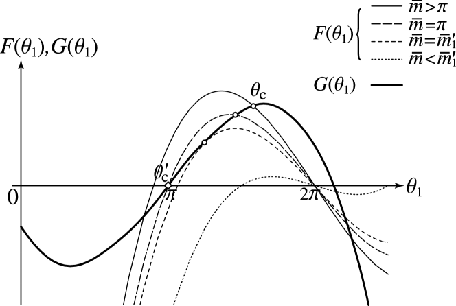
Figure 5: Curves of the function $F(\theta_{1})$ and $G(\theta_{1})$ for $t<48\pi^{2}\frac{N-1}{N}$. The thick curve denotes $G(\theta_{1})$, and other thin curves denote $F(\theta_{1})$ for various typical values of $\bar{m}$. The intersection marked by “$\circ$”, which lies in the range of $\pi\leq\theta_{1}\leq 2\pi$ for $\bar{m}\geq\bar{m}_{1}^{\prime}$, corresponds to the type III solution of $\theta_{1}=\theta_{c}$. The other intersection marked by “$\diamond$”, which appears in the range of $\pi\leq\theta_{1}\leq 2\pi$ for $\bar{m}_{1}^{\prime}\leq\bar{m}\leq\pi$, corresponds to the unstable solution of $\theta_{1}=\theta_{c}^{\prime}$.