General brane geometries from scalar potentials: gauged supergravities and accelerating universes

Abstract:

We find broad classes of solutions to the field equations for $d$-dimensional gravity coupled to an antisymmetric tensor of arbitrary rank and a scalar field with non-vanishing potential. For an exponential potential we find solutions corresponding to brane geometries, generalizing the black $p$-branes and S-branes known for the case of vanishing potential. These geometries are singular at the origin with up to two horizons. When the singularity has negative tension or the cosmological constant is positive we find time-dependent configurations describing accelerating universes. Special cases give explicit brane geometries for gauged supergravities in various dimensions, and we discuss their interrelation. Some examples lift to give new solutions to 10D supergravity. Limiting cases preserve a fraction of the supersymmetries of the vacuum. We also consider more general potentials, including sums of exponentials. Exact solutions are found for these with up to three horizons, with potentially interesting cosmological interpretation. Further examples are provided.

1 Introduction

There has been considerable study of the solutions to Einstein’s equations in the presence of the matter fields which arise within supergravity theories in four and higher dimensions. Such solutions have been invaluable to the development of our understanding of string theory, such as through the identification of the extremal limit of static black $q$-brane solutions of type-II supergravities with D-branes [1].

Although initial interest was restricted to static and/or supersymmetric solutions, late attention has turned towards constructing time-dependent solutions for the scalar-tensor-gravity system, which have been suggested to describe transitions between different vacua within string theory [2]. In particular, the decay process of unstable D-branes or D-brane–anti-D-brane pairs, such as described by the dynamics of open string tachyons, may be related at long wavelengths to time-dependent supergravity solutions called S-branes [3, 4, 5], which are extended, space-like, solitonic objects embedded within time-dependent backgrounds.

There are equally interesting potential applications to cosmology. For instance solutions exist describing time-dependent universes having contracting and expanding phases which are separated by horizons from static regions containing time-like singularities. Since observers in these universes can travel from the contracting to expanding regions without encountering the usual space-like singularities, they might ultimately lead to bouncing cosmologies. Alternatively, their expanding regions may describe accelerating cosmologies, a subject that recently has received much attention from the string community [6, 7] . These solutions appear to evade the usual singularity or no-go theorems because of the negative tension of the time-like singularities which appear [9]–[14].

The exact solutions which have been constructed to date use the field content motivated by the bosonic spectrum of low-energy string theory in ten dimensions — consisting of the metric tensor $g_{\mu\nu}$, a dilaton scalar, $\phi$, and the field strength, $F_{q+2}$, of an antisymmetric gauge form having rank $q+1$, which might arise from either the NSNS or the RR sector, and which is conformally coupled to the dilaton. For all these solutions the dilaton field is assumed to have no potential, such as is typically found for the simplest low-energy string configurations.

Our goal in the present paper is to extend these analyses to supergravity systems having nontrivial scalar potentials. We are motivated to do so because any real application of these solutions to low-energy applications (like cosmology) is likely to require a nontrivial potential for the dilaton, as well as for the other low-energy moduli. These potentials are expected to be generated in the full theory by a combination of non-perturbative effects and compactification. Indeed, several well-defined scalar potentials arise in gauged supergravities that are derived as compactified string theories with non-vanishing background fluxes. An alternative motivation is also the study of the evolution of tachyon fields, such as the open-string tachyon arising in brane-antibrane annihilation, which for a single tachyon can be written as a scalar having a nontrivial potential.

In particular, we present a systematic procedure for constructing solutions of the field equations including non-vanishing potentials. The procedure relies on introducing an ansatz which allows us to reduce the problem of solving the full field equations to the integration of a single nonlinear ordinary differential equation, whose form depends on the form of the scalar potential. This equation has solutions which permit simple analytic expressions for potentials of the generalized Liouville type

$$V\,=\,\sum_{i=1}^{L}\Lambda_{i}e^{-\lambda_{i}\phi}\,,$$ (1)

such as often arise in explicit supergravity compactifications. We therefore focus most of our attention to potentials of this type, and in particular to the simplest case where the sum is limited to only one term. (We return, however, to some more general examples in the last subsections of the paper.)

Since the paper is quite long, most readers won’t wish to read it straight through from front to back. We therefore provide here a broad road map of its layout, to facilitate better browsing. To this end we divide the remainder of our discussion into four parts. Counting the introduction you are now reading as section 1, the others are:

Section 2:

here we describe the simplest example which illustrates our mechanism of generating solutions to the Einstein/$(q+1)$-form potential/dilaton system in $q+n+2$ dimensional spacetime. We do so by the choosing an ansatz for the metric, for general $V(\phi)$, from which considerable information may be drawn about the resulting geometry. We then specialize to the Liouville potential given by (1) with a single term in the sum. This provides the simplest context within which to see how our construction works, and it already contains many supergravities of practical interest. For this potential we present broad new classes of geometries describing brane-like configurations, which for special choices of parameters reduce to those solutions which are already in the literature [15]–[21].

For these solutions we study the global properties of the geometry, and describe non-standard static brane backgrounds as well as new examples of time-dependent backgrounds having a rich global space-time structure. Many of their features follow from the study of their asymptotic behavior which, due to the non-standard form of the solution we find for the scalar field, depends both on the cosmological constant and on the conformal couplings of the dilaton to the various other fields. By studying various limits we find smooth connections with well-known asymptotically-flat geometries, including both static (Schwarzschild, Reissner-Nordström) and time-dependent (S-brane–like) configurations.

Among our static solutions we find geometries having the same global structure as have Schwarzschild, Reissner-Nordström, and AdS space-times. The time-dependent solutions include those which share the same global properties of the S-brane solutions described in [9, 2], as well as of de Sitter-like space-times (but with a time-like singularity at the origin), and of de Sitter-Schwarzschild space-times. Our solutions contain examples of time-dependent, asymptotically-flat geometries for any choice of $\Lambda$, and for a range of the conformal coupling, $\lambda$. The time-dependence of these solutions can be interpreted as being due to the presence of negative-tension time-like singularities, generalizing in this way the geometrical interpretation of [11].

We emphasize that the cosmological solutions we obtain are equally valid for either sign of the cosmological constant. It is also noteworthy that, similar to the geometries studied in [9], we find solutions which describe accelerating universes [9, 11, 22], for which the Ricci curvature vanishes at infinity due to the presence of the scalar field. This is reminiscent of some quintessence models, for which a slowly-rolling scalar field accelerates the expansion of the universe in a way which decreases to zero at asymptotically late times (in contrast with a pure cosmological constant). In this sense we furnish exact supergravity solutions which share key features of quintessence cosmologies, and which can provide a good starting point for more detailed cosmological model building.

Section 3:

in this subsection we specialize the general discussion of the Liouville potential in section 2 to the specific parameters with which this potential arises in gauged and massive supergravities in various dimensions. We do so in order of decreasing dimension, starting with the massive type-IIA supergravity in ten dimensions, including a positive cosmological constant such as has been interpreted in [1] as being due to the $vev$ of the $F_{10}$ field strength which is naturally present in the RR sector of type-IIA superstrings.

We continue to consider lower-dimensional gauged supergravities, for which the presence of a cosmological constant is a byproduct of the compactification procedure, being generated by dimensional reduction on compact (spherical or toroidal) or non-compact (hyperbolic) spaces. Our general methods applied to these specific examples give a variety of exact solutions. Some of these are already known in the literature, mainly in the form of domain walls which preserve section of the supersymmetries of the vacuum. The importance of these configurations for the study of suitable generalizations of the AdS-CFT correspondence has been noticed in [23], and is currently a field of intense study.

Our methods produce charged black brane (hole) solutions for many examples of gauged supergravities and, in general, supersymmetric domain-wall solutions are obtained from these by appropriately setting some of the parameters to zero. Interestingly, we also find cosmological configurations for some of the solutions by choosing the parameters differently. Moreover, we use general oxidation methods to lift the lower-dimensional geometries to exact solutions of a ten-dimensional theory which describes black branes wrapped about various manifolds in ten dimensions. This lifting procedure to 10 dimensions in some cases can provide connections amongst the various lower-dimensional solutions. Related black hole solutions within gauged supergravities have been studied in [24, 25].

Section 4:

this section of the paper presents the procedure which allows the generation of solutions for more general scalar potentials. Here we derive our results starting from metrics depending on two coordinates, following a treatment in five dimensions by Bowcock et al. [26] and subsequent workers [20]. This method allows us to identify the explicit functional dependence of the metric and dilaton for general potentials. Using this technique we reduce the problem of finding a brane solution to that of solving a single nonlinear ordinary differential equation for the scalar field.

This differential equation may be solved numerically given any potential, but may be solved analytically for specific kinds of potentials. We provide examples of this by deriving field configurations which solve the field equations when the scalar potential is the sum of up to three exponential terms. We also provide a few more complicated examples, such as for a flat, vanishing-charge geometry, with potential given by:

$$V(\phi)\ =\ e^{b\phi^{2}}(a-b\phi^{2})\,.$$ (2)

Finally, we end in section 5 with some general comments about our results and on possible generalizations.

2 The simplest case

We begin by describing the equations we shall solve, as well as presenting our solutions within their simplest context. Our main focus in this subsection is an exponential potential, but we first proceed as far as possible without specifying the potential explicitly. A more systematic way of generating solutions from a general potential is described in section 4, below.

2.1 The set-up

The action.

Consider the following action in $(q+n+2)$ dimensions, containing the metric, $g_{\mu\nu}$, a dilaton field, $\phi$, with a general scalar potential, $V(\phi)$, and a $(q+2)$-form field strength, $F_{q+2}={\rm d}A_{q+1}$, conformally coupled to the dilaton:

$$S=\int_{{\cal M}_{q+n+2}}d^{q+n+2}x\sqrt{|g|}\left[\alpha{\mathcal{R}}-\beta(\partial\phi)^{2}-\frac{\eta}{(q+2)!}{\rm e}^{-\sigma\phi}F^{2}_{q+2}-V(\phi)\right].$$ (3)

Here ${\mathcal{R}}$ is the Ricci scalar built from the metric, and we use MTW conventions as well as units for which $8\pi G_{d}=1$, where $G_{d}$ is the higher dimensional Newton constant.

Stability requires the constants $\alpha,\beta$, and $\eta$ to be positive and, if so, they may be removed by absorbing them into redefinitions of the fields. It is however useful to keep $\alpha$, $\beta$ and $\eta$ arbitrary since this allows us to examine the cases where each constant is taken to zero (to decouple the relevant fields). For specific values of the parameters this action can be seen as section of the low-energy string theory action, including a potential for the dilaton.

In this subsection our main application is to the Liouville potential, $V=\Lambda\,e^{-\lambda\phi}$, for which Wiltshire and collaborators [27] have shown that the equations of motion do not admit black hole solutions except for the case of a pure negative cosmological constant, $\lambda=0$ and $\Lambda<0$. Their arguments assume the fields do not blow up at infinity, and this is the condition we relax in order to find solutions. In particular we entertain scalar fields which are not asymptotically constant, but which can diverge at infinity at most logarithmically.

The equations of motion.

The field equations obtained for the action of eq. (3) are given by:

$$\left\{\begin{array}[]{l}\displaystyle\alpha G_{\mu\nu}=\beta T_{\mu\nu}[\phi]+\frac{\eta}{(q+2)!}{\rm e}^{-\sigma\phi}T_{\mu\nu}[F_{q+2}]-\frac{1}{2}V(\phi)g_{\mu\nu}\\[8.0pt] \displaystyle 2\,\beta\,\nabla^{2}\phi=-\sigma\frac{\eta}{(q+2)!}\,{\rm e}^{-\sigma\phi}F^{2}_{q+2}+\frac{d}{d\phi}V(\phi)\,,\\[8.0pt] \displaystyle\nabla_{\mu}\left({\rm e}^{-\sigma\phi}F^{\mu\cdots}\right)=0\,,\end{array}\right.$$ (4)

where

$$T_{\mu\nu}[\phi]=\nabla_{\mu}\phi\nabla_{\nu}\phi-\frac{1}{2}g_{\mu\nu}(\nabla\phi)^{2}\quad{\rm and}\quad T_{\mu\nu}[F_{q+2}]=(q+2)F_{\mu}{}^{\cdots}F_{\nu\cdots}-\frac{1}{2}g_{\mu\nu}F^{2}_{q+2}\,.$$

Since our interest is in the fields generated by extended objects charged under the $(q+1)$-form potential, we look for solutions having the symmetries of the well-known black $q$-branes. To this end we consider the following metric ansatz:

$$ds^{2}=-h(\tilde{r})dt^{2}+h(\tilde{r})^{-1}d{\tilde{r}}^{2}+\tilde{f}^{2}(\tilde{r})dx_{k,n}^{2}+\tilde{g}^{2}(\tilde{r})dy_{q}^{2}\,,$$ (5)

where $dx_{k,n}^{2}$ describes the metric of an $n$-dimensional maximally-symmetric space with constant curvature $k=-1,0,1$ and $dy_{q}^{2}$ describes the flat spatial $q$-brane directions. In addition we take the $q$-brane charge to generate a $(q+2)$-form field which depends only on $\tilde{r}$ and which is proportional to the volume form in the $(t,\tilde{r},y)$ directions, and we assume a $\tilde{r}$-dependent dilaton field.

With these choices the field equations for the antisymmetric tensor imply

$$F^{{\tilde{r}}ty_{1}\cdots y_{q}}=\frac{Qe^{\sigma\phi}}{\tilde{f}^{n}\tilde{g}^{q}}\,\epsilon^{{\tilde{r}}ty_{1}\cdots y_{q}}\,,$$ (6)

and the dilaton and Einstein equations reduce to the following system

$$2\beta\tilde{f}^{2n}\,\left[\tilde{f}^{n}\tilde{g}^{q}h\phi^{\prime}\right]^{\prime}=\tilde{f}^{n}\tilde{g}^{q}\left(\sigma\eta Q^{2}e^{\sigma\phi}+\tilde{f}^{2n}\frac{dV}{d\phi}\right),$$ (7)

and

$$n\,\frac{\tilde{f}^{\prime\prime}}{\tilde{f}}+q\,\frac{\tilde{g}^{\prime\prime}}{\tilde{g}} = -\frac{\beta}{\alpha}\left(\phi^{\prime}\right)^{2}$$

$$-\alpha\tilde{f}^{n}\,\left[h\tilde{g}^{q}\left(\tilde{f}^{n}\right)^{\prime}\right]^{\prime} = -n(n-1)\alpha k{\tilde{f}}^{2n-2}\tilde{g}^{q}+\frac{n}{d-2}V(\phi)\tilde{f}^{2n}\tilde{g}^{q}+\frac{\eta\,n(q+1)}{d-2}Q^{2}\tilde{g}^{q}e^{\sigma\phi}$$

$$\alpha(d-2)\tilde{f}^{n}\left[h\tilde{f}^{n}\left(\tilde{g}^{q}\right)^{\prime}\right]^{\prime} = \eta q(d-3-q)Q^{2}g^{q}e^{\sigma\phi}-q\tilde{f}^{2n}\tilde{g}^{q}\,V(\phi)\,.$$ (8)

We arrive at a system of four differential equations for the four functions $h,\tilde{f},\tilde{g},\phi$, whose solution requires a specification of the explicit form for the potential $V(\phi)$.

It is possible, however, to go a long way without needing to specify the potential if we make a simplifying ansatz for the components of the metric. To this end let us assume the metric component $g$ can be written in the form

$$\tilde{g}=r^{c}$$ (9)

for constant $c$, and with the new variable $r$ defined by the redefinition

$$r=\tilde{f}(\tilde{r})\,.$$ (10)

It is also convenient to think of the dilaton as being a logarithmic function of $r$, with

$$\phi(r)=\mathcal{M}\,S(\ln r)\,,$$ (11)

where $\mathcal{M}$ is a constant (whose value is given explicitly below).

The solutions.

Subject to these ansätze the solutions to the previous system of equations are given by

$$ds^{2} = -h(r)dt^{2}+\frac{dr^{2}}{g(r)}+r^{2}dx_{k,n}^{2}+r^{2c}dy_{q}^{2}\,,$$ (12)

$$F^{try_{1}\dots y_{q}} = {Q}\,e^{\sigma\mathcal{M}S(\ln r)-L(\ln r)}r^{-\mathcal{M}^{2}-(N-1)}\,\epsilon^{try_{1}\dots y_{q}}\,,$$ (13)

with

$$g(r)=h(r)\,r^{-2(N-1)}\,e^{-2L(\ln r)}\,,$$ (14)

and the function $L(\ln r)$ is given in terms of $S(\ln r)$ by

$${dL\over dx}(x)=\frac{\beta}{\alpha}\ \left({dS\over dx}(x)\right)^{2}.$$ (15)

Finally, the constants $\mathcal{M}$ and $N$ are related to the parameters $n$, $q$ and $c$ by

$$\mathcal{M}^{2}=n+cq\,,\qquad N=\frac{n+c^{2}q}{\mathcal{M}^{2}}\,.$$ (16)

So far we have not had to give the form for the scalar potential, but this cannot be avoided if the remaining unspecified functions $S(\ln r)$ and $h(r)$ are to be obtained explicitly. In principle, once $V(\phi)$ is given these remaining functions may be found by solving the remaining field equations. Before doing so it is instructive first to extract as much information as we can about the geometries which result in a potential-independent way.

Our ansätze allow the following general conclusions to be drawn:

1. The solutions describe a flat $q$-dimensional extended object or $q$-brane. In particular the metric of eq. (12) has the symmetry $\mathop{\rm SO}\nolimits(1,1)\times O_{k}(n)\times\mathop{\rm ISO}\nolimits(q)$, where $O_{k}(n)$ refers to $\mathop{\rm SO}\nolimits(1,n-1)$, $\mathop{\rm ISO}\nolimits(n)$ or $\mathop{\rm SO}\nolimits(n)$ for $k=-1,0,1$ respectively.

2. The coordinates used break down for those $r$ which satisfy $h(r)=0$. These surfaces correspond to regular horizons rather than to curvature singularities. Their number is given by the number of sign changes in $h(r)$, which is one or two for most of the cases we discuss below.

3. Typically the limit $r\to 0$ represents a real singularity, and often describes the position of the extended object which sources the geometry. The charge and tension of this source may be read off from the fields it generates, just as for Gauss’ Law in electromagnetism. For the $(q+1)$-form gauge potential this leads to charge $Q$.

4. The tension of the source may be determined using the Komar formalism, following the methods discussed in [11]. In general the result depends on the radius at which the fields are evaluated, since the gravitational and other fields can themselves carry energy. The tension calculated using the metric (12) at the space-like hypersurface at fixed $r$, turns out to be given by

   $$\mathcal{T}=\frac{C\alpha\,V_{n+q}}{2}\,r^{n+cq}\sqrt{\frac{g}{h}}\,h^{\prime}(r)\,,$$ (17)

   where $C$ is a normalization constant and $V_{n+q}$ is the volume of the $(n+q)$-dimensional constant-$r$ hypersurface over which the integration is performed.

   When the geometry is static for large $r$, the tension calculated in this way tends to the ADM mass as $r\to\infty$ provided one chooses $C=4$. For solutions for which the large-$r$ regime is time-dependent there are typically horizons behind which the geometry is static, and this formula can be used there to calculate the tension as a function of position.

5. Given the existence of horizons it is possible to formally associate a “temperature” with the static regions by identifying the periodicity of the euclidean subsection which is nonsingular at the horizon (see ref. [11]). For the metric of eq. (12) the result is

   $$T=\sqrt{\frac{g(r_{h})}{h(r_{h})}}\frac{h^{\prime}(r_{h})}{4\pi}\,,$$ (18)

   where $r_{h}$ corresponds to the horizon’s position. Notice that eq. (14) ensures that $g(r_{h})/h(r_{h})$ is nonsingular even though $h(r_{h})$ vanishes. An entropy associated with this temperature can also be computed in the same fashion as was done in [11] with a similar result.

6. The Ricci scalar is given by the comparatively simple expression

   $$\mathcal{R}=g(r)\frac{(\mathcal{M}\,S^{\prime}(\ln r))^{2}}{2\,r^{2}}+\frac{(n+q+2)V(\phi)}{n+q}+\frac{(q+2-n)\,\eta\,Q^{2}h(r)}{(n+q)\,g(r)}e^{\sigma\mathcal{M}S(\ln r)}r^{2(1-n-N)}\,.$$ (19)

   With this expression it is straightforward to check how the Ricci scalar behaves at infinity. In particular, we shall find that $\mathcal{R}$ vanishes asymptotically for many solutions, when we have a non-constant scalar field with a Liouville potential.

7. An arbitrary constant can always be added to the functional form of $\phi$, as this can always be absorbed into the other constants. When the potential has more than one term and it has an extremum, there will be an automatic solution corresponding to standard dS or AdS, depending on the sign of the potential at the critical point.

It is important to stress that all the above conclusions may be drawn independently of the choice of the potential.

To proceed further, however, we must choose a particular form for $V(\phi)$. In the next few subsections we specialize to the Liouville potential

$$V(\phi)\ =\ \Lambda e^{-\lambda\phi}\,,$$ (20)

which has the twin virtues of being simple enough to allow explicit solutions and of being of practical interest due to its frequent appearance in real supergravity lagrangians. We return in section 4 to more general choices for $V(\phi)$. As we shall see in the next subsection this simple potential is already rich enough to provide geometries having many interesting global properties.

For the Liouville potential the Einstein equations determine the dilaton function, $S(\ln r)$, to be:

$$S(\ln r)=\rho\ln r\,.$$ (21)

where the parameter $\rho$ is a proportionality constant to be determined. This form in turn implies $L(\ln r)\ =\frac{\beta}{\alpha}\rho^{2}\ln r$. Using these expressions in the remaining field equations in general implies the function $h(r)$ is over-determined inasmuch as it must satisfy two independent equations. The next subsection shows in detail how these equations admit solutions of the form:

$$h(r)=\sum_{j=1}^{4}\alpha_{j}r^{a_{j}}$$ (22)

where the coefficients $\alpha_{i}$ and $a_{i}$ are determined in terms of the parameters $k,Q^{2},\Lambda_{i}$ and an integration constant, $M$, to be defined below.

2.2 Explicit brane solutions for single Liouville potential

In this subsection, we present four classes of solutions for the Liouville potential (20), with $\Lambda\neq 0$.

Let us start by rewriting the general form of the solutions in this case, substituting in (12) and (14) the form of $S$ given by formula (21). We find in this way:

$$ds^{2} = -h(r)dt^{2}+\frac{dr^{2}}{g(r)}+r^{2}dx_{k,n}^{2}+r^{2c}dy_{q}^{2}\,,$$ (23)

$$\phi(r) = \rho\,\mathcal{M}\,\ln r\,,$$ (24)

$$F^{try_{1}\dots y_{q}} = Q\,r^{\sigma\rho\mathcal{M}-N-\mathcal{M}^{2}-\beta\rho^{2}/\alpha+1}\,\epsilon^{try_{1}\dots y_{q}}\,,$$ (25)

with

$$g(r)=h(r)\,r^{-2(N+\beta\rho^{2}/\alpha-1)}\,.$$ (26)

With these expressions the $(tt)$ and $(rr)$ components of Einstein’s equations imply the following condition for $h$:

$$\mathcal{M}^{2}\,h(r) = \left[\frac{n(n-1)\,k}{(\mathcal{M}^{2}-2+N+\beta\rho^{2}/\alpha)}\right]r^{2(\beta\rho^{2}/\alpha+N-1)}-2M\,\mathcal{M}^{2}r^{N+\beta\rho^{2}/\alpha-\mathcal{M}^{2}}-$$ (27)

$$-\left[\frac{\eta Q^{2}}{\alpha(\sigma\rho\mathcal{M}-2n+\mathcal{M}^{2}+N+\beta\rho^{2}/\alpha)}\right]{r^{\sigma\rho\mathcal{M}+2\beta\rho^{2}/\alpha}\over r^{2(n-N)}}-$$

$$-\left[\frac{\Lambda}{\alpha(\mathcal{M}^{2}+N+\beta\rho^{2}/\alpha-\lambda\rho\mathcal{M}])}\right]\frac{r^{2(N+\beta\rho^{2}/\alpha)}}{r^{\lambda\rho\mathcal{M}}}\,,$$

where $M$ is an integration constant. On the other hand the dilaton equation implies $h(r)$ must also satisfy:

$$\mathcal{M}\,h(r) = -2M\,\mathcal{M}\,r^{N+\beta\rho^{2}/\alpha-\mathcal{M}^{2}}{+}\left[\frac{\eta\,\sigma\,Q^{2}}{2\beta\rho(\sigma\rho\mathcal{M}-2n+\mathcal{M}^{2}+N+\beta\rho^{2}/\alpha)}\right]{r^{\sigma\rho\mathcal{M}+2\beta\rho^{2}/\alpha}\over r^{2(n-N)}}{-}$$ (28)

$$-\left[\frac{\lambda\Lambda}{2\beta\rho(\mathcal{M}^{2}+N+\beta\rho^{2}/\alpha-\lambda\rho\mathcal{M})}\right]\frac{r^{2(N+\beta\rho^{2}/\alpha)}}{r^{\lambda\rho\mathcal{M}}}\,.$$

The $(y_{q}y_{r})$ components of the Einstein equations impose the further conditions

$$q\cdot(c-1)\left[\frac{n(n-1)\,k}{\mathcal{M}^{2}}-\frac{\eta Q^{2}}{\alpha\mathcal{M}^{2}}r^{\sigma\rho\mathcal{M}-2(n-1)}-\frac{\Lambda}{\alpha\mathcal{M}^{2}}r^{-\lambda\rho\mathcal{M}+2}\right]=$$ (29)

$$= q\cdot\left[(n-1)\,k-\frac{\eta Q^{2}}{\alpha}r^{\sigma\rho\mathcal{M}-2(n-1)}\right].\qquad$$

We write explicit factors of $q$ on both sides of this last equation to emphasize that these equations only exist when $q\neq 0$.

In order to obtain solutions we must require that eqs. (27) and (28) imply consistent conditions for $h(r)$, and we must also impose eq. (29). We find these conditions can be satisfied by making appropriate choices for the parameters in the solutions. We identify four classes of possibilities which we now enumerate, giving interesting solutions for extended objects.

Class I.

Here we choose $k=0$ and match the coefficients of $\Lambda$ and $Q^{2}$ in formulas (27) and (28). For $q=0$, this class corresponds to the one considered in [17]. For $q\neq 0$, the condition (29) implies that $c=1$ and $Q=0$ in order to have brane-like solutions.

Class II.

In this case we take $k\neq 0$ and identify the exponents of $r$ in the terms proportional to $\Lambda$ and $k$ in (27), allowing these two terms to be merged together. Next, we identify the two remaining terms in (27) with the two terms of (28). For $q=0$ we need not impose (29) and the resulting solutions can have nonzero $Q$ [16, 17]. By contrast, for $q\neq 0$ eq. (29) implies $Q=0$ (but $c\neq 1$).

Class III.

Here we demand that the terms proportional to $Q^{2}$ and $k$ in (27) share the same power of $r$ and so combine together. If $q\neq 0$ then we also impose eq. (29), which implies $c=1$. For $q=0$ the solutions have the same form, but without the constraint coming from (29).

Class IV.

In this case we ask to fuse together the terms proportional to $k$, $\Lambda$, and $Q^{2}$ in (27) (and the same for the terms proportional to $\Lambda$ and $Q^{2}$ in (28)), by asking them to share the same power of $r$. We then identify the remaining term of (27) with the one of (28). When $q\neq 0$, we impose also (29).

Naturally, solutions belonging to different classes above can coincide for some choices of parameters. We now present these solutions in more detail. For brevity we display explicitly only the form of the metric coefficient $h(r)$ for the solutions, since the expressions for the function $g(r)$, the scalar $\phi$, and the antisymmetric forms are easily obtained using formulae (24), (25), (26).

Class I.

This class contains solutions only for $k=0$ (that is, for flat maximally-symmetric $n$-dimensional submanifolds). To obtain solutions we must also impose the following relations among the parameters:

$$\left\{\begin{array}[]{l}\alpha\sigma\mathcal{M}=-2\beta\rho\,,\\[3.0pt] \alpha\lambda\mathcal{M}=2\beta\rho\,,\\[3.0pt] c=1\quad{\rm and}\quad Q=0\quad{\rm if}\quad q\neq 0\,.\end{array}\right.$$ (30)

The first two of these imply the solution only exists of the lagrangian couplings satisfy $\sigma=-\lambda$. They also determine the parameter $\rho$ of the dilaton ansatz in terms of these couplings: $\rho=\alpha\lambda\mathcal{M}/(2\beta)$. Moreover, if $q\neq 0$, we must also require $c=1$ and $Q=0$ as specified by the last condition. For $q=0$, $Q$ need not vanish. For either choice of $q$ we have $N=1$.

With these choices the metric function $h$ becomes

$$h(r)=-2Mr^{1-\mathcal{M}^{2}+\beta\rho^{2}/\alpha}-\frac{\Lambda r^{2}}{\alpha\,\mathcal{M}^{2}\,[\mathcal{M}^{2}{-}\beta\rho^{2}/\alpha{+}1]}-\frac{\eta\,Q^{2}}{\alpha\,\mathcal{M}^{2}[\mathcal{M}^{2}{-}2n{-}\beta\rho^{2}/\alpha{+}1]\,r^{2(n-1)}}\,.$$ (31)

Class II.

This class contains geometries having any curvature $k=0,\pm 1$. The parameters of the ansatz must satisfy the constraints:

$$\left\{\begin{array}[]{l}\lambda\rho\mathcal{M}=2\,,\\[3.0pt] \alpha\sigma\mathcal{M}=-2\beta\rho\,,\\[3.0pt] \displaystyle\Lambda=\frac{\alpha\sigma\,n(n-1)\,k}{\sigma+\lambda}\,,\\[8.0pt] \displaystyle q\cdot c=\frac{-2n\lambda+n\sigma}{q(\sigma+\lambda)-\lambda\,n)}\cdot q\,,\\[8.0pt] q\cdot Q=0\,.\end{array}\right.$$ (32)

Consistency of the first two of these equations implies the condition $\alpha\sigma\lambda\mathcal{M}^{2}+4\beta=0$, and $\rho^{2}=-{\alpha\sigma}/{\beta\lambda}$. The function $h$ then becomes

$$h(r)=-2Mr^{N-\mathcal{M}^{2}+\beta\rho^{2}/\alpha}-\frac{\lambda\Lambda\,r^{2(\beta\rho^{2}/\alpha+N-1)}}{2\beta\rho\,\mathcal{M}[\mathcal{M}^{2}{-}2{+}\beta\rho^{2}/\alpha{+}N]}-\frac{\eta\,Q^{2}\,r^{2(N-n)}}{\alpha\mathcal{M}^{2}[\mathcal{M}^{2}{+}N{-}2n{-}\beta\rho^{2}/\alpha]}\,.$$ (33)

Class III.

This class of solutions is new — to our knowledge — and turns out to be among the most interesting in our later applications. It allows geometries for any $k$ and for any $q$, with the constraints

$$\left\{\begin{array}[]{l}\sigma\rho\mathcal{M}=2(n-1)\,,\\[3.0pt] \alpha\lambda\mathcal{M}=2\beta\rho\,,\\[3.0pt] \displaystyle Q^{2}=\frac{\alpha\lambda\,n(n-1)k}{\eta(\lambda+\sigma)}\,,\\[8.0pt] c=1\\[3.0pt] q\cdot\sigma=q\cdot\lambda(n-1)\,.\end{array}\right.$$ (34)

Consistency of the first two equations implies $\alpha\sigma\lambda\mathcal{M}^{2}=4(n-1)\beta$, which for $c=1$ implies the constraint $\alpha\sigma\lambda(n+q)=4(n-1)\beta$. (If $q\neq 0$ and $n\neq 1$ then $\sigma$ can be eliminated from this last condition using the final equation of (34), leading to the restriction: $\alpha\lambda^{2}(n+q)=4\beta$.)

The ansatz parameter $\rho$ then satisfies $\rho^{2}=\frac{\alpha\lambda(n-1)}{\sigma\beta}$ and $N=1$. When $Q\neq 0$ there are solutions only when $k$ is nonzero and shares the sign of $(n-1)\lambda/(\lambda+\sigma)$. For vanishing charge, $Q=0$, on the other hand, there are only solutions for $k=0$ (if $n(n-1)\lambda$ does not vanish).

The metric function $h$ of eq. (12) then becomes

$$h(r)=-2Mr^{1-\mathcal{M}^{2}+\beta\rho^{2}/\alpha}-\frac{\Lambda\,r^{2}}{\alpha\mathcal{M}^{2}[\mathcal{M}^{2}-\beta\rho^{2}/\alpha+1]}+\frac{\sigma\eta\,Q^{2}\,r^{2\beta\rho^{2}/\alpha}}{2\beta\rho\,\mathcal{M}\,[\mathcal{M}^{2}-1+\beta\rho^{2}/\alpha]}\,.$$ (35)

Class IV.

We subdivide this class into two cases, corresponding to $k=0$ and $k\neq 0$.

$\bullet$

The constraints in this case are

$$\left\{\begin{array}[]{l}\displaystyle\rho\mathcal{M}=\frac{2n}{(\sigma+\lambda)}\,,\\[3.0pt] \displaystyle\eta Q^{2}\left(\frac{\beta}{\alpha}+\frac{n}{\rho^{2}}-\frac{\lambda\mathcal{M}}{2\rho}\right)+\Lambda\left(\frac{\beta}{\alpha}-\frac{\lambda\mathcal{M}}{2\rho}\right)=0\,,\\[3.0pt] \displaystyle c=\frac{2\beta\rho\,(1+\alpha\mathcal{M}\,[1+n])+\sigma\alpha\mathcal{M}}{2\beta\rho\,(1+\alpha\mathcal{M}\,[1-q])+\sigma\alpha\mathcal{M}}\,.\end{array}\right.$$ (36)

The function $h(r)$ is then given by

$$h(r)=-2Mr^{N-\mathcal{M}^{2}+\beta\rho^{2}/\alpha}-\frac{\left[\eta\,Q^{2}+\Lambda\right]\,r^{2\beta\rho^{2}/\alpha+2N-\lambda\rho\mathcal{M}}}{\alpha\mathcal{M}^{2}[\mathcal{M}^{2}+N+\beta\rho^{2}/\alpha-2n+\sigma\rho\mathcal{M}]}\,.$$ (37)

$\bullet$

In this case, the constraints are more restrictive:

$$\left\{\begin{array}[]{l}\displaystyle\lambda\rho\mathcal{M}=2\,,\\[8.0pt] \displaystyle\sigma\rho\mathcal{M}=2(n-1)\,,\\[8.0pt] \displaystyle\eta Q^{2}\left(\frac{\beta}{\alpha}+\frac{n-1}{\rho^{2}}\right)+\Lambda\left(\frac{\beta}{\alpha}-\frac{1}{\rho^{2}}\right)=\frac{n(n-1)\beta}{2}k+\,,\\[8.0pt] \displaystyle q\cdot\left[\alpha\,(n-1)\,k\,[n\,(c-1)-\mathcal{M}^{2}]-\eta\,Q^{2}\,[c-1-\mathcal{M}^{2}]=\Lambda\,(c-1)\right]\,.\end{array}\right.$$ (38)

Consistency of the first two requires $\sigma=\lambda(n-1)$, and the parameter $\rho$ is given by $\rho=2/(\lambda\mathcal{M})$.

The function $h$ reduces to

$$h(r)=-2Mr^{N-\mathcal{M}^{2}+\beta\rho^{2}/\alpha}+\frac{\left[\alpha\,n(n-1)\,k-\eta\,Q^{2}-\Lambda\right]\,r^{2\beta\rho^{2}/\alpha+2N-2}}{\alpha\mathcal{M}^{2}[\mathcal{M}^{2}-2+\beta\rho^{2}/\alpha+N]}\,.$$ (39)

Properties of the solutions

In this subsection, we describe the global properties of the geometries we have obtained. In particular, since $r$ is the coordinate on which the metric depends, whether the metric is time-dependent or not hinges on whether or not $r$ is a time-like or space-like coordinate. This in turn depends on the overall sign of $h(r)$, and section of our purpose is to identify how this sign depends on position in the space, and on the parameters of the solution.

We shall find that the presence of the Liouville potential allows much more complicated structure for the charged dilatonic geometries than is obtained without a potential. In particular we wish to follow how the geometry is influenced by the sign of the cosmological constant $\Lambda$, by the size of the conformal couplings of the dilaton, $\sigma,\lambda$, and by the curvature parameter, $k$, of the $n$-dimensional submanifold.

The solutions to our equations with $V(\phi)=0$ are studied in ref. [11], who found that the geometries having $n$-dimensional $k=1$ submanifolds are the well known static $q$-brane configurations, with at most two horizons. By contrast, those configurations with $k=0$ or $-1$ subspaces describe time-dependent geometries separated from static regions by horizons. These have been argued to correspond to special cases of S-brane configurations.

Here we find that the addition of the Liouville potential modifies this earlier analysis in several interesting ways. In general, we find that if $\Lambda<0$ the background is usually static, regardless of the choice of the curvature $k$ of the subspace. There can be interesting exceptions to this statement, however, for sufficiently large conformal couplings to the dilaton. These exceptional solutions are quite appealing for cosmological applications, since they correspond to time-dependent backgrounds even in the presence of a Liouville potential with negative sign (that is the typical situation when one considers compact gauged supergravities).

If $\Lambda>0$, on the other hand, we have examples of new geometries which are de Sitter-like, although they are not asymptotically de Sitter, due to the presence of the dilaton. Instead the Ricci scalar asymptotically vanishes, although in most cases the Riemann tensor itself does not. These asymptotic geometries are intriguing because in them observers experience a particle horizon. This asymptotic joint evolution of the dilaton and metric resembles what happens in quintessence cosmologies, and in this sense our solutions may lead to connections between supergravity and quintessence models. Among these asymptotically time-dependent backgrounds, we find examples in which an event horizon hides a space-like singularities from external observers. (This is an important difference relative to the existing S-brane geometries, which have time-like singularities from which asymptotic observers can receive signals).

For the remainder of the discussion we analyze each of the first three classes in turn. In each case we start with an initial overview of the main global features and then specialize to the limit $\Lambda\to 0$, allowing us to see how the new geometries relate to those which were previously known. In some cases we find in this way generalizations of the earlier S-brane configurations. In other cases we instead find less well-known static geometries. We end each case by focusing on a four dimensional example in detail, since this exposes the geometries in their simplest and clearest forms. In the following, we also limit our discussion to the cases $q=0$ (i.e. to zero-branes) and $M\geq 0$, although the relaxation of these assumptions is straightforward to perform.

Class I.

As is clear from the expression for $h(r)$, the global properties of the geometry are therefore largely controlled by the value of the parameter $\rho$, which itself depends on the value of the conformal coupling, $\lambda$, of the dilaton in the scalar potential. We now consider the various possibilities. When $0<\beta\rho^{2}<\alpha\,(n+1)$ the options depend on the sign of $\Lambda$. If $\Lambda<0$, $r$ is a spatial coordinate and the geometry is static. By contrast, it is time dependent for positive $\Lambda$.

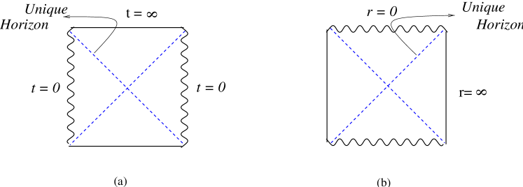
Figure 1: Penrose diagram for $(a)$ a de Sitter–S-brane-like geometry and $(b)$ a Schwarzschild–anti-de Sitter-like geometry. The scalar potential prevents the solutions from being asymptotically flat.

The number of horizons similarly depends on the sign of the scalar potential. For $\Lambda<0$, the static solutions can have (depending on the values of $M$ and $Q$) zero, one or two horizons, respectively corresponding to the causal structure of the AdS, Schwarzschild-AdS, or Reissner-Nordström-AdS geometries. For $\Lambda>0$, on the other hand, the time-dependent solutions can have at most one cosmological horizon, and always have a naked singularity at the origin (figure 1). Consequently, these time-dependent geometries violate the Penrose cosmic censorship hypothesis, which might give one pause regarding their stability against gravitational perturbations.

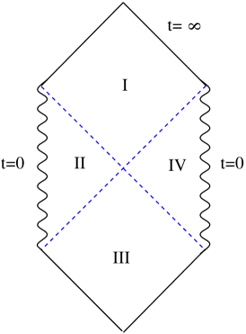
Figure 2: Penrose diagram for an S-brane.

The situation is different if $\beta\rho^{2}>\alpha\,(n+1)$. In this case the geometry is always asymptotically flat and asymptotically time-dependent, for most choices of $\Lambda$. The causal structure for this geometry is illustrated by the Penrose diagram of figure 2. All of the solutions in this class also share a naked singularity at $r=0$.

For $\Lambda\to 0$, the solutions in this class reduce directly to the solutions found in [9, 11] for $k=q=0$. The solutions are therefore asymptotically flat in this limit, and their Penrose diagram is the same as for an S-brane, see figure 2. This shows there is a smooth connection between the S-brane solutions with and without a Liouville potential, and our new solutions potentially acquire an interpretation as the supergravity description of a decay of a non-BPS brane, or a $D-\bar{D}$ system to the same degree that this is true in the $\Lambda=0$ case.

For sufficiently negative $\Lambda$ this example shows explicitly how, for proper choice of the conformal couplings, the addition of a negative potential converts the solution into an asymptotically static, rather than time-dependent, one. The Penrose diagram in the static case becomes figure 3.

Figure 3: Penrose diagram for some of our solutions. The causal structure is like that of an anti-de Sitter-Reissner-Nordström Black hole $(a)$, or its extremal limit $(b)$.

Let us now discuss in detail a specific four-dimensional example, where the various global properties just discussed can be made explicit in a transparent way.

A four dimensional example.

Consider in detail the 4D case corresponding to $n=2$ and $q=0$, corresponding to a point source with three transverse dimensions. We therefore also have $\mathcal{M}^{2}=2$ and $N=1$. Since $q=0$, we are free to choose $Q$ arbitrarily (unlike the requirement $Q=0$ which follow if $q\neq 0$). If we use the standard normalizations, $\alpha=1$ and $\beta=1/2$, $\eta=1/4$, then with the Class I consistency condition $\sigma=-\lambda$ we may take $\lambda$ and $\Lambda$ as the only free parameters in the lagrangian.

In this case the metric is

$$ds^{2}=-h(r)dt^{2}+\frac{dr^{2}}{g(r)}+r^{2}dx_{2}^{2}\,,$$ (40)

with

$$h(r)=-2Mr^{\frac{\rho^{2}}{2}-1}+\frac{Q^{2}}{4(1+\frac{\rho^{2}}{2})}\frac{1}{r^{2}}-\frac{\Lambda r^{2}}{(6-\rho^{2})}$$ (41)

and

$$g(r)=h(r)r^{-\rho^{2}}\,,$$ (42)

where the parameter $\rho$ is given by $\rho=\lambda\sqrt{2}$. The dilaton and gauge fields are similarly given by (11), (13) with the appropriate choices for the various parameters. We suppose, for the time being, that the parameters $\Lambda$, $M$, and $Q$ are all nonzero.

Consider first the case where the geometry is asymptotically static, corresponding to $\Lambda<0$ and $\rho^{2}<6$. In this case we have a space-time with the same conformal structure as the Reissner-Nordström geometry. This configuration admits an extremal limit in which the event and Cauchy horizons coincide. Since the Hawking temperature for the extremal configuration vanishes, one might ask whether the extremal geometry can be supersymmetric and stable. In the next subsections we answer the supersymmetric question by embedding the solution into particular gauged supergravities for which the supersymmetry transformations are known, and find the extremal configurations break all of the supersymmetries. As such it need not be stable either, although we have not performed a detailed stability analysis. There are choices for which the solution (41) can leave some supersymmetries unbroken, however. For instance this occurs for the domain wall configuration obtained by sending both $M$ and $Q$ to zero.

Let us now specialize to the case $\Lambda>0$. It is then easy to see that the Ricci scalar, ${\mathcal{R}}$, for this geometry vanishes at large $r$ whenever $\rho^{2}>0$. The Ricci tensor, on the other hand, does not always similarly vanish asymptotically, and we have three different cases:

• When $0\leq\rho^{2}\leq 2$ the Ricci tensor does not vanish at infinity, and so the geometry is asymptotically neither flat nor a vacuum spacetime ($R_{\mu\nu}=0$). The geometry is then asymptotically time dependent, with a Cauchy horizon and a pair of naked singularities and a Penrose diagram given by figure 1$a$.

• For $2<\rho^{2}<6$ the Ricci tensor vanishes at infinity, but the geometry is nevertheless not asymptotically flat since the Riemann tensor is nonzero at infinity. The spacetime’s causal structure is much as in the previous case.

• When $\rho^{2}>6$, the geometry is asymptotically flat and time-dependent, with the Penrose diagram of figure 2. Notice that in this case the time-dependence of the metric is not due to the scalar potential, but instead arises from the choice of the sign of integration constants. In particular, the geometry is time dependent for positive $M$, and also in the case $\Lambda<0$.

The interesting feature of this example is that it brings out how the asymptotic properties change with the choice of $\rho$. It also shows that the geometries can be asymptotically time-dependent even when the scalar potential is negative (corresponding to AdS-like curvatures). These solutions share the Penrose diagram — figure 2 – of the S-brane geometries of ref. [11], and in this way generalize these to negative scalar potentials. The geometry shares the naked singularities having negative tension of the S-brane configurations, and we expect many of the arguments developed in that paper to go over to the present case in whole cloth.

Class II.

Solutions belonging to this class are similar to — but not identical with — the ones of the previous class. Choosing $\Lambda<0$ we again find static solutions with at most two horizons (as for figure 3). When $\Lambda>0$, on the other hand, we have asymptotically time-dependent solutions with at most one horizon and a naked singularity at the origin. It is also not possible to obtain an asymptotically flat configuration for either sign of $\Lambda$ or for any choice of the conformal coupling. When $\Lambda\to 0$, these solutions again reduce to the asymptotically-flat S-brane geometries of [11].

A four dimensional example.

Specializing to 4 dimensions we choose $n=2$ and $q=0$, and so $\mathcal{M}^{2}=2$ and $N=1$. Since $q=0$, $Q$ can remain arbitrary. With the conventional choices $\alpha=1$, $\beta=1/2$ and $\eta=1/4$, the consistency condition $\alpha\sigma\lambda\mathcal{M}^{2}+4\beta=0$ requires $\sigma=-1/\lambda$, leaving as free parameters $\lambda$, $\Lambda$, and the integration constants $M$ and $Q$. The constant $\rho$ is then given by $\rho=\sqrt{2}/\lambda$.

With these choices the metric becomes

$$ds^{2}=-h(r)dt^{2}+\frac{dr^{2}}{g(r)}+r^{2}dx_{2}^{2}\,,$$ (43)

with

$$h(r)=-2Mr^{\frac{\rho^{2}}{2}-1}-\frac{\Lambda r^{\rho^{2}}}{\rho^{2}\left[1+\frac{\rho^{2}}{2}\right]}+\frac{Q^{2}}{4\left[1+\frac{\rho^{2}}{2}\right]r^{2}}\,,$$ (44)

and

$$g(r)=h(r)r^{-\rho^{2}}\,.$$ (45)

As before the expressions for the scalar and the 2-form field strength are easily obtained from formulae (11), (13), with the appropriate substitutions of parameters. From eq. (44) it is clear that the term proportional to $\Lambda$ is dominant for large $r$ for all $\rho^{2}>0$. This means that for $\Lambda<0$ we have a static solution for large $r$, while for $\Lambda>0$ it is time-dependent in this limit.

Class III.

This class contains the most interesting new time-dependent configurations. Here, as in Class I, the asymptotic properties of the geometry depend on the choice of the parameter $\rho$, and so ultimately also on the conformal couplings.

Consider first $\beta\rho^{2}<\alpha$. For $\Lambda<0$ this gives static configurations with at most one horizon — which are neither asymptotically flat nor asymptotically AdS — having the same conformal structure as Schwarzschild-AdS black branes. For $\Lambda>0$ by contrast the solution is asymptotically time dependent (but not asymptotically flat) and can have up to two horizons, implying the same conformal structure as for a Schwarzschild-de Sitter black hole (see figure 4). Interestingly, these properties imply an asymptotically time-dependent configuration, but without naked singularities.

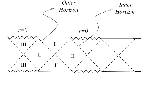
Figure 4: The Penrose diagram for $\Lambda>0$ Class III solutions, which resembles the same for a Schwarzschild-de Sitter black hole geometry.

If, however, $\beta\rho^{2}>\alpha$ then the choice $\Lambda>0$ instead gives static configurations having at most one horizon. Choosing $\Lambda<0$ also gives solutions are which are static, although for these one finds at most two horizons if $\beta\rho^{2}>\alpha(n+1)$, or only one horizon if $\alpha<\beta\rho^{2}<\alpha(n+1)$.

These solutions do not reduce to Ricci-flat space-times in the limit $\Lambda\to 0$. This limit instead gives a class of non-standard black brane solutions, which are included among the general class of solutions found in [28] (and were interpreted in [29] in terms of unstable branes).

A four dimensional example.

We now specialize to the 4-dimensions with the choice $n=2$ and $q=0$, implying $\mathcal{M}^{2}=2$ and $N=1$. Just as was true for Class II, the usual choices $\alpha=1$, $\beta=1/2$ and $\eta=1/4$ in this case imply that the consistency condition $\alpha\sigma\lambda(n+q)=4(n-1)\beta$ reduces to $\sigma=1/\lambda$. Unlike for Class II, however, the expression for $\rho$ may be solved, giving $\rho=\lambda\sqrt{2}$.

The metric becomes:

$$ds^{2}=-h(r)dt^{2}+\frac{dr^{2}}{g(r)}+r^{2}dx_{2}^{2}\,,$$ (46)

with

$$h(r)=-2Mr^{\frac{\rho^{2}}{2}-1}-\frac{\Lambda\,r^{2}}{(6-\rho^{2})}+\frac{Q^{2}\,r^{\rho^{2}}}{\rho^{2}(2+\rho^{2})}$$ (47)

and

$$g(r)=h(r)r^{-\rho^{2}}\,,$$ (48)

and the expressions for the scalar and the form are found from formulae (11), (13) specialized to the relevant parameter values.

We now focus on the asymptotically time-dependent geometries since these are qualitatively new, and since the asymptotically-static solutions are similar to those found in the previous classes. To this end consider the case $\rho^{2}<2$ and $\Lambda>0$, for which the metric is asymptotically time dependent with horizons which cover the geometry’s space-like singularities.

With these choices the Ricci scalar vanishes at infinity (although the Ricci tensor does not so long as $\rho\neq 0$), and so the metric is neither asymptotically flat nor asymptotically a vacuum spacetime. Neither is it asymptotically de Sitter, even though $\Lambda>0$, but it is instead a kind of interpolation between a de Sitter geometry and an S-brane configuration.

The Penrose diagram for the geometry resembles that of a de Sitter-Schwarzschild space-time, as in figure 4, for which the hiding of the singularities by the horizons is clear. This satisfies the cosmic censorship conjecture, and one might hope it to be stable against the perturbations which were argued [13] to potentially destabilize the $\Lambda=0$ S-brane configuration.

The asymptotically time-dependent regions of the geometries are those labelled by I and I’ in figure 4. In region I’ the spatial geometry contracts as one moves into the future, while in region I the spatial geometry expands. As the figure makes clear, it is possible to pass smoothly from the contracting to the expanding region without ever meeting the singularities. Remarkably, neither does one pass through a region of matter satisfying an unphysical equation of state, such as is typically required to produce a bouncing FRW universe. We believe it to be worthwhile trying to extend these geometries (perhaps to higher dimensions) to construct more realistic bouncing cosmologies without naked singularities or unphysical matter.

3 Gauged and massive supergravities

The exponential Liouville potential we consider above has many practical applications because it frequently arises in the bosonic sector of gauged supergravities. However the solutions we construct require specific relations to hold amongst the various conformal couplings of the general action, (3), and it must be checked that these are consistent with supersymmetry before interpreting our geometries as solving the field equations of any particular supergravity.

In this subsection we verify that many extended supergravities do satisfy the required conditions, and by so doing find numerous solutions to specific supergravity models. We find that many of these describe the field configurations due to extended objects in the corresponding supergravity.

Some of the supergravities we consider have well-established string pedigrees inasmuch as they can be obtained as consistent truncations of ten-dimensional type-IIA and IIB supergravities, which themselves arise within the low-energy limit of string theory. This allows the corresponding solutions to be lifted to ten dimensions, and so they themselves may be interpreted as bona fide low-energy string configurations. It also allows them to be related to each other and to new solutions using the many symmetries of string theory such as T-duality and S-duality.

We organize our discussion in the order of decreasing dimension, considering the 10-, 8-, 7-, 6-, 5- and 4-dimensional cases. Among these we consider examples of massive, compact-gauged and non-compact-gauged supergravities. Of these the study of compact gauged supergravities is particularly interesting due to its relation with extensions of the AdS-CFT correspondence. On the other hand it is the non-compact gauged supergravities which are most likely to have cosmological applications.

3.1 Massive supergravity in 10 dimensions

Romans [30] has shown how to construct a ten-dimensional supergravity theory which has an exponential scalar potential for the dilaton, and we take this as our first example. The solution we obtain in this case was earlier obtained in refs. [31, 32].

The bosonic fields of the theory comprise the metric, a scalar, and 2-form, 3-form and 4-form field strengths, $F_{2}={\rm d}A_{1}$, $F_{3}={\rm d}A_{3}$ and $F_{4}={\rm d}A_{3}$. The equations of motion for all of the fields is trivially satisfied if we set all of their field strengths to zero, leaving only the dilaton and the metric. The relevant action for these fields is [32]:

$$S=\int d^{10}x\sqrt{|g|}\left[R-\frac{1}{2}(\partial\phi)^{2}-\frac{1}{2}m^{2}{e}^{5\phi/2}\right]$$ (49)

which is a special form of eq. (3) obtained by choosing $\alpha=1$, $\beta=\frac{1}{2}$, $\Lambda=\frac{1}{2}\,m^{2}$ and $\lambda=-5/2$. Notice we need not specify either $\eta$ or $\sigma$ since we may turn off the gauge form field simply by choosing $Q=0$.

To obtain a solution we choose $q=0$, and from the relation $n+q+2=10$ we have immediately $n=8$. We find a solution in Class I, for $k=0$, with $\mathcal{M}^{2}=8$ and $\rho=2\sqrt{2}\lambda=-5\sqrt{2}$. This leads to the following solution (which is the same as discussed in [31])

$$ds_{10}^{2} = -h(r)dt^{2}+\frac{r^{50}}{h(r)}dr^{2}+r^{2}dx_{0,8}^{2}$$

$$\phi(r) = -20\ln r$$ (50)

where

$$h(r)=\frac{m^{2}}{256}r^{2}-2Mr^{18}\,.$$ (51)

For $M>0$ this solution is time-dependent for large $r$, and has a horizon at $r^{16}=m^{2}/(512M)$. It is interesting to note that we would obtain an asymptotically time-dependent configuration even if the scalar potential were to be negative, due to the dominance at large $r$ of the term proportional to $M$. The geometry in this case is asymptotically flat, and the Penrose diagram is the same as for an S-brane solution, shown in figure 2.

The case $M=0$ corresponds instead to a static space-time, and a particularly interesting one at that since a straightforward check reveals that it is supersymmetric since it admits a Killing spinor preserving half of the supersymmetries of the action. In this case, the metric becomes (after a constant rescaling of the eight internal spatial coordinates):

$$ds_{10}^{2}=h(r)\,\eta_{\mu\nu}dx^{\mu}dx^{\nu}+\frac{r^{50}}{h(r)}dr^{2}\,.$$ (52)

In this case the solution belongs to the family discussed in section 3.2 of [32], the so-called “domain wall” solution. Notice also that original $\mathop{\rm SO}\nolimits(8)\times\mathop{\rm SO}\nolimits(1,1)$ symmetry is promoted in this case to $\mathop{\rm SO}\nolimits(1,8)\times{\mathbb{R}}$, where ${\mathbb{R}}$ denotes translation symmetry in the $r$ direction.

3.2 Gauged supergravity in 8 dimensions

We next consider Salam-Sezgin gauged supergravity in eight dimensions [33]. In general, the bosonic part of the action consists of the metric, a dilatonic scalar, five scalars parameterizing the coset $\mathop{\rm SL}\nolimits(3,\mathbb{R})/\mathop{\rm SO}\nolimits(3)$ (and so consisting of a $3\times 3$ unimodular matrix, $L$), an $\mathop{\rm SU}\nolimits(2)$ gauge potential and a three-form potential $C_{\it 3}$. We further restrict ourselves to a reduced bosonic system where the $\mathop{\rm SU}\nolimits(2)$ gauge fields vanish, and we take $L$ to be a constant diagonal matrix.

The action for the remaining bosonic fields can be written

$$S=\int d^{8}x\sqrt{|g|}\left[\frac{1}{4}R-\frac{1}{2}(\partial\phi)^{2}-\frac{1}{48}e^{2\phi}G_{\mu\nu\lambda\sigma}G^{\mu\nu\lambda\sigma}+{\rm g}^{2}e^{-2\phi}\right]\,,$$ (53)

and so we read off $\alpha=1/4$, $\beta=\eta=1/2$, $\sigma=-2$, $\Lambda=-{\rm g}^{2}$ and $\lambda=2$. The 3-form potential couples to $q=2$ branes, so in $n+q+2=8$ dimensions we have $n=4$.

In this case we can find solutions in class I, since this model satisfies the appropriate consistency condition $\sigma=-\lambda$. Consequently $k=0$ and since $q\neq 0$ the solution also has $c=1$ and describes fields for 2-branes carrying vanishing charge, $Q=0$. With these values we find $\mathcal{M}^{2}=6$, $N=1$ and $\rho$ is predicted to be $\rho=\sqrt{3/2}$, and the solution takes the following form:

$$ds_{8}^{2} = -h(r)dt^{2}+r^{2}dx_{0,4}^{2}+\frac{r^{6}}{h(r)}dr^{2}+r^{2}dy_{2}^{2}\,,$$ (54)

$$\phi(r) = 3\ln r\,,$$ (55)

$$h(r) = -\frac{2M}{r^{2}}+\frac{{\rm g}^{2}r^{2}}{6}\,.$$ (56)

This geometry correspond to an uncharged black 2-brane, and has at most one horizon. The causal structure of the geometry resembles the AdS-Schwarzschild black hole. These field configurations turn out to be supersymmetric only when $M=Q=0$.

Uplifting procedure.

Because this supergravity can be obtained by consistently truncating a higher-dimensional theory, this solution also directly gives a solution to the higher-dimensional field equations. We now briefly describe the resulting uplift to 11 dimensions, following the procedure spelled out in [33]. The corresponding 11-dimensional metric and 4-form are,

$$ds_{11}^{2}=e^{-2\phi/3}ds_{8}^{2}+e^{4\phi/3}(d\Omega_{3})^{2}\,,$$ (57)

or,

$$ds_{11}^{2}=-\frac{h(r)}{r^{2}}dt^{2}+dx_{4}^{2}+dy_{2}^{2}+\frac{r^{4}}{h(r)}dr^{2}+r^{4}(d\Omega_{3})^{2}\,.$$ (58)

The form of this 11-dimensional solution makes it clear why the choice $M=Q=0$ is supersymmetric, because in this case the preceding metric describes flat 11-dimensional space.

3.3 Gauged supergravity in 7 dimensions

In this subsection we present two kinds of solutions to the 7-dimensional $\mathcal{N}=2$ gauged supergravity with $\mathop{\rm SU}\nolimits(2)$ gauge symmetry studied in [34]. The bosonic part of the theory contains the metric tensor, a scalar $\phi$, $\mathop{\rm SU}\nolimits(2)$ gauge fields, $A^{I}_{\mu}$, with field strengths, $F^{I}_{\mu\nu}$, and a 3-form gauge potential, $C_{\mu\nu\rho}$, with field strength $G_{\mu\nu\lambda\rho}$. The bosonic action for the theory is [34]:

$${\rm e}^{-1}\mathcal{L}=R-\frac{1}{2}(\partial\phi)^{2}-\frac{1}{4}e^{\frac{4}{\sqrt{10}}\,\phi}G_{\mu\nu\lambda\rho}G^{\mu\nu\lambda\rho}-\frac{1}{4}e^{-\frac{2}{\sqrt{10}}\phi}F^{I}_{\mu\nu}F^{I\,\mu\nu}+4{\rm g}^{2}e^{\frac{2}{\sqrt{10}}\phi}+\frac{1}{4}{\rm e}^{-1}F^{I}_{\emph{2}}\wedge F^{I}_{\emph{2}}\wedge A_{\emph{3}}\,,$$ (59)

where ‘${\rm e}$’ corresponds to the determinant of the 7-bein, and ${\rm g}$ is the gauge coupling of the $\mathop{\rm SU}\nolimits(2)$ gauge group. From this action we read off $\alpha=1$, $\beta=1/2$, $\Lambda=-4{\rm g}^{2}$ and $\lambda=-2/\sqrt{10}$.

We now consider the following two kinds of solution to this theory, which differ by whether it is the 2-form, $F^{I}_{\emph{2}}$, or the 4-form, $G_{\emph{4}}$, which is nonzero. In either of these cases a great simplification is the vanishing of the Chern-Simon terms vanish.

3.3.1 Solutions with excited $F^{I}_{\emph{2}}$

The solution for to nonzero $F_{\emph{2}}^{I}$ corresponds to the field sourced by a point-like object, $q=0$, and so $n+q+2=7$ implies $n=5$. This particular tensor field satisfies $\eta=\frac{1}{2}$ and $\sigma=2/\sqrt{10}=-\lambda$.

Since $\sigma=-\lambda$ we look for solutions belonging to Class I. For these $k=0$, $Q$ is not constrained because $q=0$. Also $\mathcal{M}^{2}=5$, $N=1$ and the parameter $\rho=\lambda\mathcal{M}=-\sqrt{2}$. The corresponding metric takes the form

$$ds_{7}^{2}=-h(r)dt^{2}+r^{2}dx_{0,5}^{2}+\frac{r^{2}}{h(r)}dr^{2}\,,$$ (60)

with metric coefficients, scalar and 2-form field strength given by

$$h(r) = -\frac{2M}{r^{3}}+\frac{4{\rm g}^{2}}{25}r^{2}+\frac{Q^{2}}{50\,r^{8}}$$ (61)

$$\phi(r) = -\sqrt{10}\ln r$$ (62)

$$F^{\rm tr} = \frac{Q}{r^{8}}\epsilon^{\rm tr}\,.$$ (63)

This solution is static and corresponds to a charged black hole in seven dimensions. It can have up to two horizons corresponding to the two zeros of $h(r)$, which can be explicitly found as

$$h(r)=\frac{4{\rm g}^{2}}{25\,r^{8}}\left(-\frac{50M}{4{\rm g}^{2}}+r^{10}+\frac{Q^{2}}{8{\rm g}^{2}}\right)=\frac{4{\rm g}^{2}}{25\,r^{8}}(X-X_{1})(X-X_{2})\,,$$ (64)

where $X=r^{5}$ and

$$X_{1,2}=\frac{25M}{4{\rm g}^{2}}\pm\frac{1}{2{\rm g}}\sqrt{\frac{(25M)^{2}}{4{\rm g}^{2}}-\frac{Q^{2}}{2}}\,.$$ (65)

From here is clear that there would be an extremal solution when $Q=\frac{25M}{\sqrt{2}{\rm g}}$. One can further check that the above field configuration becomes supersymmetric if the parameters $M$ and $Q$ are taken to zero. Notice that this supersymmetric configuration is not the extremal configuration, for which the two horizons coincide at a double zero of $h(r)$.

Uplifting procedure.

Following [35] this solution can be oxidized on a three sphere $S^{3}$ to give a solution to ten dimensional IIB supergravity. This 10D theory contains a graviton, a scalar field, and the NSNS 3-form among other fields, and has a ten dimensional action (in the Einstein frame) given by

$$S_{10}=\int d^{10}x\sqrt{|g|}\left[\frac{1}{4}R-\frac{1}{2}(\partial\phi)^{2}-\frac{1}{12}\,e^{-2\phi}H_{\mu\nu\lambda}H^{\mu\nu\lambda}\right]\,.$$ (66)

We perform some conventional rescalings to convert to the conventions of [35], after which we have a ten dimensional configuration given by

$${}ds_{10}^{2} = \left(\frac{2}{r}\right)^{3/4}\left[ds_{7}^{2}\right]+\left(\frac{r}{2}\right)^{5/4}\left[d\theta^{2}+d\psi^{2}+d\varphi^{2}+(d\psi+\cos\theta d\varphi-\frac{Q}{5r^{5}}dt)^{2}\right],$$

$$\phi = -\frac{5}{4}\,\log\frac{r}{2}\,,$$

$$H_{3} = -\frac{Q}{r^{6}}\,{\rm d}r\wedge{\rm d}t\wedge({\rm d}\psi+\cos\theta{\rm d}\varphi)-\frac{{\rm g}}{\sqrt{2}}\sin\theta\,{\rm d}\theta\wedge{\rm d}\varphi\wedge{\rm d}\psi\,.$$ (67)

where $ds_{7}^{2}$ corresponds to the solution given in eq. (60). This uplifted 10-dimensional solution describes NS-5 branes intersecting with fundamental strings in the time direction.

S-duality.

For a later comparison with the uplifted solution of 6-dimensional supergravity, it is convenient to rewrite this 10-dimensional solution by performing a change of variables and a new re-scaling of the parameters. For the same reason, it is also useful to perform in this subsubsection an S-duality transformation of this solution.

As a first step to this end, let us make the manipulation of the angular variables of the three sphere simpler by introducing the following left-invariant 1-forms of $\mathop{\rm SU}\nolimits(2)$:

$$\sigma_{1} = \cos\psi\,{\rm d}\theta+\sin\psi\sin\theta\,{\rm d}\varphi\,,$$

$$\sigma_{2} = \sin\psi\,{\rm d}\theta-\cos\psi\sin\theta\,{\rm d}\varphi\,,$$

$$\sigma_{3} = {\rm d}\psi+\cos\theta\,{\rm d}\varphi\,,$$ (68)

and

$$h_{3}=\sigma_{3}-\frac{Q}{5}\frac{1}{r^{5}}\,{\rm d}t\,.$$ (69)

Next, we perform the following change of variables

$$\begin{array}[b]{rclrclrclrcl}\displaystyle\frac{r}{2}&=&\rho^{\frac{4}{5}}\,,&t&=&\displaystyle\frac{5}{32}\,\tilde{t}\,,&{\rm d}x_{4}&=&\displaystyle\frac{1}{2\sqrt{2}}\,{\rm d}\tilde{x}_{4}\hskip 8.5359pt\,,&{\rm d}x_{5}&=&\displaystyle\frac{1}{2}\,{\rm d}Z\\ {\rm g}&=&\sqrt{2}\,\tilde{{\rm g}}\,,&Q&=&\sqrt{2}\,2^{7}\,\tilde{Q}\,,&\sigma_{i}&=&\displaystyle\frac{1}{\tilde{{\rm g}}}\,\tilde{\sigma}_{i}\,.&&&\end{array}$$ (70)

It is straightforward to check that the 10-dimensional solution (3.3.1) becomes, after these changes

$$d\tilde{s}_{10}^{2} = \frac{1}{2}\,\rho^{-1}\,\left[d\tilde{s}_{6}^{2}\right]+\frac{\rho}{\tilde{{\rm g}}^{2}}\left[\tilde{\sigma}_{1}^{2}+\tilde{\sigma}_{2}^{2}+\left(\tilde{\sigma}_{3}-\frac{\tilde{{\rm g}}\tilde{Q}}{4\sqrt{2}}\frac{1}{\rho^{4}}d\tilde{t}\right)^{2}\right]+\rho\,dZ^{2}\,,$$

$$\phi = -\ln\rho\,,$$

$$H_{\emph{3}} = -\frac{1}{\tilde{{\rm g}}^{2}}\tilde{\sigma}_{1}\wedge\tilde{\sigma}_{2}\wedge\tilde{h}_{3}+\frac{\tilde{Q}}{\sqrt{2}\,\tilde{{\rm g}}\,\rho^{5}}{\rm d}\tilde{t}\wedge{\rm d}\rho\wedge\tilde{h}_{3}\,,$$ (71)

where we define

$$d\tilde{s}_{6}^{2}=-\tilde{h}(\rho)\,d\,\tilde{t}^{2}+\frac{\rho^{2}}{\tilde{h}(\rho)}d\,\rho^{2}+\rho^{2}\,d\tilde{x}_{0,4}^{2}$$ (72)

and, after re-scaling $M$,

$$\tilde{h}=-\frac{2\tilde{M}}{\rho^{2}}+\frac{\tilde{g}^{2}}{32}\rho^{2}+\frac{\tilde{Q}^{2}}{8}\frac{1}{\rho^{6}}\,.$$ (73)

We now transform the solution from the Einstein to the string frame (and denote all string-frame fields with a bar). This leads to

$$d\bar{s}_{10}^{2} = \frac{1}{2}\,\rho^{-2}\,\left[d\tilde{s}_{6}^{2}\right]+\frac{1}{\tilde{{\rm g}}^{2}}\left[\tilde{\sigma}_{1}^{2}+\tilde{\sigma}_{2}^{2}+\left(\tilde{\sigma}_{3}-\frac{\tilde{{\rm g}}\tilde{Q}}{4\sqrt{2}}\frac{1}{\rho^{4}}d\tilde{t}\right)^{2}\right]+dZ^{2}\,,$$

$$\bar{\phi} = -2\ln\rho\,,$$

$$\bar{H_{\emph{3}}} = H_{\emph{3}}\,.$$ (74)

We have a solution to 10-dimensional IIB supergravity with a nontrivial NSNS field. If we perform an S-duality transformation to this solution we again obtain a solution to type-IIB theory but with a nontrivial RR 3-form, $F_{\emph{3}}$. The S-duality transformation acts only on the metric and on the dilaton, leaving invariant the three form. In this way we are led to the following configuration, which is S-dual to the one derived above

$$d\bar{s}_{10}^{2} = \frac{1}{2}\,\,\left[d\tilde{s}_{6}^{2}\right]+\frac{\rho^{2}}{\tilde{{\rm g}}^{2}}\left[\tilde{\sigma}_{1}^{2}+\tilde{\sigma}_{2}^{2}+\left(\tilde{\sigma}_{3}-\frac{\tilde{{\rm g}}\tilde{Q}}{4\sqrt{2}}\frac{1}{\rho^{4}}d\tilde{t}\right)^{2}\right]+\rho^{2}\,dZ^{2}\,,$$

$$\bar{\phi} = 2\ln\rho\,,$$

$$F_{\emph{3}} = H_{\emph{3}}\,.$$ (75)

This form is particularly convenient for making the comparison with our later uplifted solution to 6-dimensional supergravity.

3.3.2 Solution with excited $G_{\emph{4}}$

We can also apply our ansatz to obtain a solution to 7-dimensional supergravity which sources the 3-form potential, $A_{\emph{3}}$, for which we have $q=2$ and so $n=5-q=3$. The 3-form couplings in the lagrangian are $\eta=6$ and $\sigma=-4/\sqrt{10}=2\lambda$.

These couplings allow solutions belonging to Class III, and so for which $c=1$, $\mathcal{M}^{2}=5$, $N=1$, and $\rho=\lambda\mathcal{M}=-1/\sqrt{2}$. Formulae (34) allow two possible curvatures for the $n=3$ dimensional symmetric subspace. It is either spherical ($k=1$) and the brane charge is $Q^{2}=1/3$, or it is flat ($k=0$) with brane charge $Q=0$.

For the spherical case, the metric takes the form

$$ds_{7}^{2}=-h(r)dt^{2}+r^{2}dx_{1,3}^{2}+\frac{r^{2}}{h(r)}dr^{2}+r^{2}dy^{2}_{2}\,,$$ (76)

and the metric coefficients, the scalar and the 2-form field are

$$h(r) = -\frac{2M}{r^{3}}+\left(\frac{4{\rm g}^{2}}{25}+\frac{12\,Q^{2}}{25}\right)r^{2}$$ (77)

$$\phi(r) = -\sqrt{10}\ln r$$ (78)

$$F^{try_{1}y_{2}} = \frac{Q}{r^{2}}\epsilon^{try_{1}y_{2}}\,.$$ (79)

This geometry is static an possesses only one horizon. It describes a charged black 2-brane in seven dimensions, for which the special case $M=Q=0$ is supersymmetric (and coincides with this same limit of the solution of the previous subsubsection). The uplifting to 10 dimensions can be done straightforwardly by first dualising the $G_{\emph{4}}$ field in seven dimensions to transform it into a 3-field, and then applying the prescription given in ref. [35].

3.4 Romans’ 6-dimensional gauged supergravity

The next two subsections consider two kinds of gauged supergravity in six dimensions. We start here with Romans’ $N=4^{g}$ 6D supergravity, which was oxidized to 10 dimensions in ref. [36].

Romans’ [37] 6-dimensional $N=4^{g}$ gauged supergravity is non-chiral and has ${\mathcal{N}}=4$ supersymmetries. The bosonic part of the theory consists of a graviton, three $\mathop{\rm SU}\nolimits(2)$ gauge potentials, $A_{\mu}^{I}$, an abelian gauge potential, ${\mathcal{A}}_{\mu}$, a 2-form gauge potential, $B_{\mu\nu}$, and a scalar field, $\phi$. Our starting point is the following consistently reduced version of this action [38]:

$$S = \int d^{6}x\sqrt{|g|}\Bigg{[}\frac{1}{4}R-\frac{1}{2}(\partial\phi)^{2}-\frac{1}{4}e^{-\sqrt{2}\,\phi}({\mathcal{F}}_{\mu\nu}{\mathcal{F}}^{\mu\nu}+F_{\mu\nu}^{I}F^{I\,\,\mu\nu})-\frac{1}{12}e^{2\sqrt{2}\phi}G_{\mu\nu\rho}G^{\mu\nu\rho}+$$ (80)

$$\hphantom{\int d^{6}x\sqrt{|g|}\Bigg{[}}\!+\frac{{\rm g}^{2}}{8}e^{\sqrt{2}\phi}-\frac{1}{8\sqrt{|g|}}\,\epsilon^{\mu\nu\rho\sigma\tau\kappa}B_{\mu\nu}({\mathcal{F}}_{\rho\sigma}{\mathcal{F}}_{\tau\kappa}+F^{I}_{\rho\sigma}F^{I}_{\tau\kappa})\Bigg{]}\,.$$

Here, ${\rm g}$ is the coupling constant of the $\mathop{\rm SU}\nolimits(2)$ group, and $\epsilon^{\mu\nu\rho\sigma\tau\kappa}$ is the usual Levi-Civita tensor density. $F^{I}_{\emph{2}}$ denotes the $\mathop{\rm SU}\nolimits(2)$ gauge field strength, while ${\mathcal{F}}_{\emph{2}}={\rm d}{\mathcal{A}}_{\emph{1}}$ and $G_{\emph{3}}={\rm d}B_{\emph{2}}$ are the abelian field strengths for the abelian potential and the antisymmetric field. The supersymmetry transformations with these conventions may be found, for instance, in [38]. This action leads to the choices $\alpha=1/4$, $\beta=1/2$, $\Lambda=-{\rm g}^{2}/8$ and $\lambda=-\sqrt{2}$.

We consider in turn two cases which differ in which gauge potential is excited by the solution. We first take this to be the 2-form potential, $B_{\emph{2}}$, and then choose it to be one of the 1-form potentials, $A^{I}_{\mu}$ or ${\mathcal{A}}_{\mu}$. In this second case the solution looks the same for either choice of embedding within the gauge group, although the supersymmetry of the result can differ.

3.4.1 Solutions with excited $G_{\emph{3}}$

We first consider a charged string which sources the field $B_{\it 2}$, and so for which $q=1$, $n=4-q=3$ and the dilaton couplings are $\eta=1/2$ and $\sigma=-2\sqrt{2}=2\lambda$. These couplings allow solution belonging to Class III, implying $c=1$, $\mathcal{M}^{2}=4$, $N=1$ and $\rho=-1/\sqrt{2}$. The curvature of the $n=3$ dimensional subspace can be $k=1$ if $Q^{2}=1$, or it is flat if $Q^{2}=0$.

For the case $k=1$ the metric takes the form

$$ds_{6}^{2}=-h(r)dt^{2}+r^{2}dx_{1,3}^{2}+\frac{r^{2}}{h(r)}dr^{2}+r^{2}dy^{2}$$ (81)

with metric coefficients, scalar and 2-form field given by

$$h(r) = -\frac{2M}{r^{2}}+\frac{{\rm g}^{2}}{32}r^{2}+\frac{Q^{2}}{2}r^{2}\,,$$ (82)

$$\phi(r) = -\sqrt{2}\ln r\,,$$ (83)

$$G^{try} = \frac{Q}{r}\epsilon^{try}\,.$$ (84)

The geometry describes the fields of a charged black string in six dimensions. In the limit where $M$ and $Q$ vanish, (and so for which the symmetric 3-dimensional subspace is flat) the solution preserves half of the supersymmetries of the action.

Uplifting procedure.

Ref. [36] shows how to lift any solution of the massive 6-dimensional Romans’ theory to a solution of 10-dimensional massive IIA supergravity compactified on $S^{3}\times T^{1}$. This was extended to the massless $N=4^{g}$ case in ref. [38], which is the one of present interest.

The bosonic part of the relevant 10-dimensional supergravity theory is

$${\mathcal{L}_{10}}=\tilde{R}-\frac{1}{2}(\partial\phi)^{2}-\frac{1}{2}e^{-\frac{1}{2}\tilde{\phi}}\tilde{F}_{\mu\nu\rho\lambda}\tilde{F}^{\mu\nu\rho\lambda}\,.$$ (85)

From this one can show that the right ansatz to uplift our solution to ten dimensions is given by

$$d\tilde{s}^{2}_{10} = \frac{1}{2}e^{\frac{\sqrt{2}}{4}\phi}ds^{2}_{6}+\frac{1}{{\rm g}^{2}}e^{-\frac{3\sqrt{2}}{4}\phi}\sum_{i=1}^{3}\left(\sigma^{i}-\frac{{\rm g}\,A^{i}_{1}}{\sqrt{2}}\right)^{2}+e^{\frac{5\sqrt{2}}{4}\phi}dZ^{2}\,,$$ (86)

$$\tilde{F}_{\emph{4}} = \left(H_{\emph{3}}-\frac{1}{{\rm g}^{2}}h^{1}\wedge h^{2}\wedge h^{3}+\frac{1}{{\rm g}\sqrt{2}}F^{i}_{2}\wedge h^{i}\right)\wedge{\rm d}Z\,,$$ (87)

$$\tilde{\phi} = \frac{1}{\sqrt{2}}\,\phi\,,$$ (88)

where $h^{i}=\sigma^{i}-{1}/{\sqrt{2}}{\rm g}A^{i}_{1}$, $\sigma^{i}$ are left-invariant 1-forms for $\mathop{\rm SU}\nolimits(2)$. The 3-form, $H_{\emph{3}}$, appearing within the expression for the 4-form is the 6-dimensional dual [38],

$$H_{\mu\nu\rho}=\frac{1}{6}e^{2\sqrt{2}\phi}e\,\epsilon_{\mu\nu\rho\lambda\beta\gamma}G^{\lambda\beta\gamma}\,,$$ (89)

of the 3-form field strength of the field ${\rm d}B$ appearing in eq. (80).

Substituting our solution with excited $B_{\mu\nu}$ field, we find for $H_{\emph{3}}$

$$H_{x_{1}x_{2}x_{3}} = Q\,r^{4}\,e^{2\sqrt{2}\phi}\epsilon_{x_{1}x_{2}x_{3}}\,,$$ (90)

$$d\tilde{s}^{2}_{10} = \frac{1}{2\sqrt{r}}\left(-h(r)dt^{2}+\frac{r^{2}\,dr^{2}}{h(r)}+r^{2}dx^{2}_{1,3}+r^{2}dy^{2}\right)+$$ (91)

$$+\frac{1}{4{\rm g}^{2}r^{3/2}}\left(d\theta^{2}+d\varphi^{2}+d\psi^{2}+2\cos\theta\,d\psi\,d\varphi\right)+\frac{1}{r^{5/2}}dZ^{2}\,,$$

$$\tilde{F}_{\emph{4}} = Q\,e^{2\sqrt{2}\,\phi}\,r^{4}{\rm d}x_{1}\wedge{\rm d}x_{2}\wedge{\rm d}x_{3}\wedge{\rm d}Z-\frac{1}{{\rm g}^{2}}\sin\theta\,{\rm d}\varphi\wedge{\rm d}\theta\wedge{\rm d}\psi\wedge{\rm d}Z\,,$$ (92)

$$\tilde{\phi} = -\ln r\,.$$ (93)

This solution can be interpreted as a D4-brane extending along the $y$-direction, with the three angles parameterising the 3-sphere ($dx_{1,3}^{2}$ in the six dimensional metric), intersecting with a D2-brane extended along the $y,Z$ directions, with the intersection describing a string.

3.4.2 Solutions with excited $F_{\emph{2}}$ or ${\mathcal{F}}_{\emph{2}}$

These two cases can be treated together, since these fields appear in the action (80) with the same conformal couplings: $\eta=1/2$, $\sigma=\sqrt{2}=-\lambda$, and $q=0$ for which $n=4$. These parameters suggest solution in Class I, for which the $n=4$-dimensional spatial dimensions are flat, $k=0$, $\mathcal{M}^{2}=4$, $N=1$ and $\rho=-1/\sqrt{2}$.

The solution in this case takes the form

$$ds_{6}^{2} = -h(r)dt^{2}+r^{2}dx_{0,4}^{2}+\frac{r^{2}}{h(r)}dr^{2}\,,$$ (94)

$$\phi(r) = -\sqrt{2}\ln r\,,$$ (95)

$$F^{\rm tr} = \frac{Q}{r^{7}}\,\epsilon^{\rm tr}\,,$$ (96)

where

$$h(r)=-\frac{2M}{r^{2}}+\frac{{\rm g}^{2}r^{2}}{32}+\frac{Q^{2}}{8r^{6}}\,.$$ (97)

This geometry describes the fields due to a point source (0-brane) in 6 dimensions, whose causal structure resembles that of an AdS-Reissner-Nördstrom black hole. There can be at most two horizons and a time-like singularity at the origin. The position of the horizons are obtained from the positive roots of the function $h(r)$, which in this case can be written

$$h(r)=\frac{{\rm g}^{2}}{32\,r^{6}}\left[r^{8}-\frac{64\,M}{{\rm g}^{2}}r^{4}+\frac{4\,Q^{2}}{{\rm g}^{2}}\right]=\frac{{\rm g}^{2}}{32\,r^{6}}(X-X_{1})(X-X_{2})\,,$$ (98)

where $X\equiv r^{4}$, and the roots are

$$r^{4}_{1,2}=X_{1,2}=\frac{32M}{{\rm g}^{2}}\pm\frac{1}{2{\rm g}}\sqrt{\frac{(64M)^{2}}{{\rm g}^{2}}-16Q^{2}}\,,$$ (99)

showing that the positions of the horizons depend on the values of $M$ and $Q$. In particular, the extremal solution is the case $16M={\rm g}Q$. An examination of the supersymmetry transformations for Romans’ gravity shows that this extremal solution is not supersymmetric, although the domain wall configuration for which $M=Q=0$ reduces to the supersymmetric solution of the previous subsubsection.

Uplifting procedure.

In this subsubsection we uplift this solution to a solution of type-IIA 10-dimensional supergravity, with nontrivial metric, dilaton and RR 4-form, $C_{4}$. Using a slight modification of a procedure described earlier, we get the 10-dimensional configuration

$$d\tilde{s}^{2}_{10} = \frac{1}{2\sqrt{r}}\left(-h(r)dt^{2}+\frac{r^{2}\,dr^{2}}{h(r)}+r^{2}dx^{2}_{0,4}\right)+$$

$$+\frac{r^{3/2}}{{\rm g}^{2}}\left((\sigma^{1})^{2}+(\sigma^{2})^{2}+\left(\sigma^{3}-\frac{{\rm g}}{\sqrt{2}}A_{t}^{(3)}\right)^{2}\right)+\frac{1}{r^{5/2}}dZ^{2}\,,$$

$$\tilde{\phi} = -\ln{r}\,,$$ (100)

$$\tilde{F}_{\emph{4}} = \left(-\frac{1}{{\rm g}^{2}}\sin\theta\,{\rm d}\theta\wedge{\rm d}\varphi\wedge{\rm d}\psi+\frac{Q}{2\sqrt{g}r^{5}}{\rm d}t\wedge{\rm d}r\wedge({\rm d}\psi+\cos\theta\,{\rm d}\varphi)\right)\wedge{\rm d}Z\,,$$

where we use the conventions of the previous subsection 3.4.1 for the definitions of variables. This 10D geometry describes D4 branes along the $x_{4}$ directions of the 6-dimensional gauged supergravity, plus two D2 branes extending along the $\psi$ and $\varphi$ directions.

T-duality.

To relate this solution to those obtained previously, we write the previous solution in the string frame (whose fields we label as before with a bar). Only the metric changes, becoming

$$d\bar{s}_{10}^{2}=\frac{1}{2}\left[ds_{6}^{2}\right]+\frac{r^{2}}{g^{2}}\left[\sigma_{1}^{2}+\sigma_{2}^{2}+\left(\sigma_{3}-\frac{g\,Q}{4\sqrt{2}}\frac{1}{r^{4}}dt\right)^{2}\right]+r^{-2}\,dZ^{2}\,.$$ (101)

This gives a solution to IIA supergravity with excited RR 4-form, $C_{\emph{4}}$. We now proceed by performing a T-duality transformation, leading to a solution of IIB theory with nontrivial RR 3-form, $C_{\emph{3}}$. The complete solution then becomes

$$d\bar{s}_{10}^{2} = \frac{1}{2}\,\,\left[ds_{6}^{2}\right]+\frac{r^{2}}{{\rm g}^{2}}\left[\sigma_{1}^{2}+\sigma_{2}^{2}+\left(\sigma_{3}-\frac{{\rm g}\,Q}{4\sqrt{2}}\frac{1}{r^{4}}dt\right)^{2}\right]+r^{2}\,dZ^{2}\,,$$ (102)

$$\bar{\phi} = 2\ln{r}$$ (103)

$$C_{\emph{3}} = -\frac{1}{{\rm g}^{2}}\sigma_{1}\wedge\sigma_{2}\wedge h_{3}-\frac{Q}{\sqrt{2}\,{\rm g}}\frac{1}{r^{5}}\,{\rm d}t\wedge{\rm d}r\wedge h_{3}\,.$$ (104)

We are led in this way to precisely the same 10D solution as we found earlier — c.f. formula (3.3.1) — which we obtained by uplifting our 7-dimensional solution to 10 dimensions. This establishes in detail the interrelationship between these solutions.

3.5 Salam-Sezgin 6-dimensional gauged supergravity

Let us now consider the chiral 6-dimensional supergravity constructed by Salam and Sezgin in [39]. This theory is potentially quite attractive for applications [40, 41] since it has a positive potential for the dilaton. For this supergravity we find de Sitter-like time-dependent solutions from Class I, which are not supersymmetric (as is expected for a time-dependent solutions). Salam-Sezgin theory has not yet been obtained as a consistent reduction of a higher-dimensional string theory, and so its string-theoretic pedigree is not yet clear. What is clear is that such a connection would be of great interest, since the solutions we find here could be used to find interesting new string geometries with potential cosmological applications.

The bosonic field content comprises the graviton, a 2-form potential, $B_{\emph{2}}$, a dilaton and various gauge potentials, $A$, (of which we focus on a single $\mathop{\rm{}U}\nolimits(1)$ factor). The bosonic lagrangian takes the form

$$e^{-1}{\mathcal{L}}_{ss}=\frac{1}{4}R-\frac{1}{4}(\partial\phi)^{2}-\frac{1}{12}e^{2\phi}G_{\mu\nu\rho}G^{\mu\nu\rho}-\frac{1}{4}e^{\phi}F_{\mu\nu}F^{\mu\nu}-\frac{1}{2}g^{2}e^{-\phi}\,,$$ (105)

where $g$ is the gauge coupling and the field strengths for $B_{\emph{2}}$ and $A$ are given by $F_{\emph{2}}={\rm d}A$ and $G_{\it 3}={\rm d}B_{\emph{2}}+F_{\emph{2}}\wedge A$. The supersymmetry transformations for this theory can be found in [39]. The parameters of interest for generating solutions are $\alpha=\beta=\frac{1}{4}$, $\Lambda=g^{2}/2$ and $\lambda=1$.

We do not have solutions within our ansätze for which the 2-form potential, $B_{\emph{2}}$, is nonzero. We do find solutions with $F_{\emph{2}}\neq 0$, for which $q=0$, $n=4$, $\eta=\frac{1}{2}$ and $\sigma=-1=-\lambda$. Solutions of Class I can describe this case, for which $k=0$ and $\rho=1$. The metric which results is

$$ds_{6}^{2} = -h(r)\,dt^{2}+\frac{r^{2}}{h(r)}dr^{2}+r^{2}dx_{0,4}^{2}\,,$$

$$\phi(r) = 2\,\ln r\,,$$

$$F^{\rm tr} = \frac{Q}{r^{7}}\epsilon^{\rm tr}\,,$$ (106)

where

$$h(r)=-\frac{2M}{r^{2}}-\frac{g^{2}\,r^{2}}{8}+\frac{Q^{2}}{8\,r^{6}}\,.$$ (107)

This function has only a single zero for real positive $r$.

Since $h(r)$ is negative for large $r$, this solution is clearly asymptotically time-dependent. Its causal structure resembles that of a de-Sitter-S-brane spacetime (figure 1$a$). Moreover, from the supersymmetry transformations, one can show that it breaks supersymmetry for all values of $M$ and $Q$.

3.6 Gauged supergravity in 5 dimensions

Romans [42] has studied a gauged supergravity in 5 dimensions, corresponding to a ${\mathcal{N}}=4$ $\mathop{\rm SU}\nolimits(2)\times\mathop{\rm{}U}\nolimits(1)$ gauged theory. The bosonic spectrum consists of gravity, a scalar, an $\mathop{\rm SU}\nolimits(2)$ Yang-Mills potential $A^{I}$ (with field strength $F_{\emph{2}}^{I}$), an abelian gauge potential $H$ with field strength $G_{\emph{2}}$, and two 2-form antisymmetric potentials, $B_{\emph{2}}$. Using the conventions of [43] we consider the reduced system without the 2-form potentials. We find for this system two classes of point-like solutions having supersymmetric limits. These solutions can be up-lifted, as shown in [43], to solutions of ten dimensional type-II supergravity.

The action in 5 dimensions is the following [43]:

$$S = \int d^{5}x\sqrt{|g|}\Biggl{[}R-\frac{1}{2}(\partial\phi)^{2}-\frac{1}{4}e^{-\frac{2}{\sqrt{6}}\phi}F_{\mu\nu}F^{\mu\nu}-\frac{1}{4}e^{\frac{4}{\sqrt{6}}\phi}G_{\mu\nu}G^{\mu\nu}+\qquad$$ (108)

$$\hphantom{\int d^{5}x\sqrt{|g|}\Biggl{[}}\!+4{\rm g}^{2}e^{\frac{2}{\sqrt{6}}\phi}-\frac{1}{4\sqrt{|g|}}\epsilon^{\mu\nu\rho\sigma\lambda}F_{\mu\nu}^{I}F_{\rho\sigma}^{I}H_{\lambda}\Biggl{]}\,,$$

where $G_{\emph{2}}={\rm d}H$ is the field strength for the $\mathop{\rm{}U}\nolimits(1)$ gauge potential, $H_{\mu}$. We have $\alpha=1$, $\beta=1/2$, $\Lambda=-4{\rm g}^{2}$ and $\lambda=-2/\sqrt{6}$. There are two cases to be considered, depending on whether one of the $F^{I}_{\it 2}$ or $G_{\emph{2}}$ which is nonzero in the solution.

3.6.1 Solutions with excited $F^{I}_{\emph{2}}$

In this case we have $q=0$, $n=3$, $\eta=1/2$ and $\sigma=2/\sqrt{6}=-\lambda$. These allow a 0-brane solution in Class I, for which $k=0$, $\mathcal{M}^{2}=3$, $N=1$ and $\rho=-\sqrt{2}$. The resulting field configuration is given by

$$ds_{5}^{2} = -h(r)dt^{2}+r^{2}dx_{0,3}^{2}+\frac{r^{2}}{h(r)}dr^{2}$$ (109)

$$\phi(r) = -\sqrt{6}\ln r$$ (110)

$$F = -\frac{Q}{r^{4}}\,{\rm d}t\wedge{\rm d}r\,,$$ (111)

with

$$h(r)=-\frac{2M}{r}+\frac{4}{9}{\rm g}^{2}r^{2}+\frac{Q^{2}}{18\,r^{4}}\,,$$ (112)

and where the gauge field is only nonzero for one of the gauge-group generators.

The causal structure of this geometry is like that of an AdS-RN black hole of positive mass, and has at most two horizons. For negative mass there are no horizons at all and the solution has a naked singularity at $r=0$. For $M>0$ the extremal limit corresponds to the case where the two roots of $h(r)$,

$$r^{3}_{1,2}=\frac{9\,M}{4\,{\rm g}^{2}}\pm\frac{1}{2}\sqrt{\left(\frac{9\,M}{2\,{\rm g}^{2}}\right)^{2}-\frac{Q^{2}}{2\,{\rm g}^{2}}}\,,$$ (113)

coincide, corresponding to when ${9\,M}/{2\,{\rm g}}={Q^{2}}/{\sqrt{2}}$, and for which the solution is static everywhere but is not supersymmetric.

A supersymmetric configuration is obtained in the totally static, uncharged case, corresponding to the choices $M=Q^{2}=0$. This represents a domain-wall-like object and preserves one of the supersymmetries of the action.

Uplifting procedure to 7 dimensions.

In this subsection we show how the lift of this 5D solution to 7 dimensions on 2-torus gives the same solution as we found in subsubsection (3.3.1). This reinforces the conclusion that the solutions we find are related to one another by dimensional reduction/oxidation, or through dualities.

To this end we denote 7-dimensional quantities with a tilde, and rescale the coordinates in the following way

$$\tilde{t}=\sqrt{\frac{25}{9}}t\,,\qquad\tilde{r}=r^{{3}/{5}}\,,\qquad d\tilde{x}_{k,3}=dx_{k,3}\,.$$ (114)

The uplifting procedure acting on the solutions then gives [43]

$$d\tilde{s}_{7}^{2} = e^{\frac{4}{5\sqrt{6}}\phi}ds_{5}^{2}+e^{-\frac{6}{5\sqrt{6}}\phi}(d\,Y^{2}+d\,Z^{2})$$

$$\tilde{\phi} = \sqrt{\frac{6}{10}}\,\phi$$

$$\tilde{G}_{4} = F_{2}\wedge{\rm d}Y\wedge{\rm d}Z$$

$$\tilde{F}_{2}^{I} = F_{2}^{I}\,.$$ (115)

Applied to the previous formulae, with the redefinition

$$\tilde{h}(\tilde{r}) = \frac{9}{25}\tilde{r}^{-\frac{4}{3}}h(\tilde{r})$$ (116)

$$= -\frac{2\tilde{M}}{\tilde{r}^{3}}+\frac{4{\rm g}^{2}\tilde{r}^{2}}{25}+\frac{Q^{2}}{50\,\tilde{r}^{8}}$$

one ends with the following 7-dimensional metric

$$d\tilde{s}_{7}^{2}=-\tilde{h}(\tilde{r})d\tilde{t}^{2}+\tilde{r}^{2}d\tilde{x}_{0,5}^{2}+\frac{\tilde{r}^{2}}{\tilde{h}(\tilde{r})}d\tilde{r}^{2}\,.$$ (117)

This is exactly the same form found in subsection (3.3). (It is straightforward to check that the other fields also transform to the fields found in the 7-dimensional case.)

Uplifting procedure to 10 dimensions.

As discussed in [43], any solution to Romans’ 5-dimensional gauged supergravity (108) can be lifted to a solution of 10-dimensional type-II string theory, with the solutions so obtained corresponding to a 5-brane wrapped in a non-trivial way.

Let us therefore consider type-IIB supergravity in 10 dimensions, for which the relevant bosonic part of the truncated action is given by

$${\mathcal{L}_{10}}=\tilde{R}-\frac{1}{2}(\partial\tilde{\phi})^{2}-\frac{1}{2}e^{-\tilde{\phi}}\tilde{F}_{\mu\nu\rho}\tilde{F}^{\mu\nu\rho}\,.$$ (118)

The complete reduction ansatz for the 10-dimensional solution compactified on $T^{1}\times S^{3}\times T^{1}$ is given by [43]

$$d\tilde{s}^{2}_{10} = e^{\frac{13}{5\sqrt{6}}\phi}ds^{2}_{5}+e^{\frac{3}{5\sqrt{6}}\phi}(dY^{2}+dZ^{2})+\frac{1}{4{\rm g}^{2}}e^{\frac{-3}{\sqrt{6}}\phi}\sum_{i=1}^{3}(\sigma^{i}-{\rm g}A_{1}^{i})^{2}\,,$$ (119)

$$\tilde{F}_{\emph{3}} = e^{\frac{4}{\sqrt{6}}\phi}*G_{\emph{2}}-\frac{1}{24\,{\rm g}^{2}}\epsilon_{ijk}\,h^{i}\wedge h^{j}\wedge h^{k}+\frac{1}{4}\sum_{i=1}^{3}F_{\emph{2}}^{i}\wedge h^{i}\,,$$ (120)

$$\tilde{\phi} = \sqrt{6}\,\phi\quad{\rm and}\quad h^{i}=\sigma^{i}-{\rm g}\,A_{\emph{1}}^{i}\,.$$ (121)

Since we choose $A_{\emph{1}}^{i}=A_{t}^{3}=A_{t}$ and $G_{\it 2}=0$ for the present purposes, the 10-dimension solution reduces to

$$h^{1}=\sigma^{1}\,,\qquad h^{2}=\sigma^{2}\,,\qquad h^{3}=\sigma^{3}-{\rm g}A_{t}\,,$$ (122)

and so

$$\phi = -\ln(r)$$ (123)

$$d\tilde{s}^{2}_{10} = \frac{1}{r^{13/5}}\left[-h(r)dt^{2}+r^{2}dx_{0,3}^{2}+\frac{r^{2}}{h(r)}dr^{2}\right]+\frac{1}{r^{3/5}}(dY^{2}+dZ^{2})+$$

$$+\frac{r^{3}}{4{\rm g}^{2}}\left[\sigma_{1}^{2}+\sigma_{2}^{2}+\left(\sigma_{3}^{2}-\frac{A_{0}}{r^{3}}dt\right)^{2}\right],$$

$$\tilde{F}_{\emph{3}} = -\frac{1}{4\,{\rm g}^{2}}\,\sin\theta\,{\rm d}\theta\wedge{\rm d}\varphi\wedge{\rm d}\psi+\frac{Q}{4r^{4}}\,{\rm d}t\wedge{\rm d}r\wedge({\rm d}\psi+\cos\theta\,{\rm d}\varphi)\,.$$ (124)

In these expressions $\sigma_{i}$ are defined as before (see eq. 3.3.1) This 10-dimensional solution to type-IIB supergravity describes an NS-5 brane, extending along the $x_{1},x_{2},x_{3},Y,Z$ directions, plus two F1 strings extending along the $\psi,\varphi$ directions.

3.6.2 Solutions with excited $G_{\emph{3}}$

In this case, we have $q=0$, $n=3$, $\eta=1/2$ and $\sigma=-4/\sqrt{6}=2\lambda$, and so we can obtain solutions of Class III. For these $k=c=1$, $\mathcal{M}^{2}=3$, $N=1$ and $\rho=-\sqrt{2}$. The metric becomes

$$ds_{5}^{2} = -h(r)dt^{2}+r^{2}dx_{1,3}^{2}+\frac{r^{2}}{h(r)}dr^{2}$$ (125)

$$\phi(r) = -\sqrt{6}\ln r$$ (126)

$$G_{\rm tr} = -Q\,r^{2}dt\wedge dr$$ (127)

with

$$h(r)=-\frac{2M}{r}+\frac{r^{2}}{9}(4\,{\rm g}^{2}+Q^{2})\,.$$ (128)

This solution has a single event horizon at $r_{h}^{3}={18M}/{(4{\rm g}^{2}+Q^{2})}$. It has the same causal structure as an AdS-Schwarzschild black hole.

This solution turns out to be supersymmetric if we choose $M$ and $Q$ equal to zero. This is the same supersymmetric solution found in subsection 3.6.1 in these limits.

Uplifting procedure to 10 dimensions.

This solution may also be lifted using eqs. (118), (119) into a full solution to type-IIB supergravity on $T^{1}\times S^{3}\times T^{1}$. In the present instance, $F_{2}^{I}=0$ and so $h^{i}=\sigma^{i}$ which implies

$$\phi = -\ln(r)$$

$$d\tilde{s}^{2}_{10} = \frac{1}{r^{13/5}}\left[-h(r)dt^{2}+r^{2}dx_{1,3}^{2}+\frac{r^{2}}{h(r)}dr^{2}\right]+\frac{1}{r^{3/5}}(dY^{2}+dZ^{2})+$$

$$+\frac{r^{3}}{4{\rm g}^{2}}[d\theta^{2}+d\varphi^{2}+d\psi^{2}+2\cos\theta\,d\psi\,d\varphi]$$

$$\tilde{F}_{\emph{3}} = \frac{Q}{r^{4}}\sin^{2}\alpha\sin\,\beta\,{\rm d}\alpha\wedge{\rm d}\beta\wedge{\rm d}\gamma-\frac{1}{24\,{\rm g}^{2}}\,\sin\theta\sin\psi\,{\rm d}\theta\wedge{\rm d}\varphi\wedge{\rm d}\psi\,.$$ (129)

Here we use the metric for the 3-sphere (inside the 5 dimensional gauged supergravity) to be

$$dx_{1,3}^{2}=d\alpha^{2}+\sin^{2}\alpha\,d\beta^{2}+\sin^{2}\alpha\sin^{2}\beta\,d\gamma^{2}$$ (130)

and we use the same conventions of subsubsection (3.6.1) in the definition of the variables. We obtain in this case a solution representing two NS-5 branes that intersect in the $Y,Z$ directions.

3.7 Non-compact gauged supergravity

The absence of de Sitter-like solutions to gauged $N=8$ 4D supergravity using compact gaugings has led to the study of non-compact and non-semi-simple gaugings, using groups like $\mathop{\rm CSO}\nolimits(p,q,r)$, such as developed in [44]. These in some cases can have de Sitter solutions. When regarded as dimensional reductions from a higher-dimensional theory, these theories correspond to reductions on hyperboloids, which give $\mathop{\rm SO}\nolimits(p,q)$ gaugings. Recent effort has been devoted to the study of possible cosmological applications of non-compact gauged supergravities [45]. In this subsubsection we present an example of non-compact gauged supergravity in four dimensions which furnishes alternative examples of the cosmological solutions we have been considering, rather than de Sitter space.

We consider the 4-dimensional model studied in [46] (see also [45]) with $\mathop{\rm SO}\nolimits(a,b)$ gauging, where $a$ and $b$ are natural numbers satisfying $a+b=8$. Let us consider a consistent truncation of the complete supergravity action describing gravity coupled to a single real scalar field:

$$S=\int d^{4}x\sqrt{|g|}\left(R-\frac{1}{2}(\partial\phi)^{2}-V_{a,b}(\phi)\right)$$ (131)

where the potential $V_{a,b}$ is given by

$$V_{a,b}=\frac{{\rm g}^{2}}{16}a\left(b-3a\right)e^{\sqrt{\frac{b}{a}}\phi}\,.$$ (132)

This action falls into our general class, with $\alpha=1$, $\beta=1/2$, $\Lambda={1}/{16}\,{\rm g}^{2}a(b-3a)$ and $\lambda=-\sqrt{b/a}$. The absence of a antisymmetric form requires the choice $Q=0$.

This action admits solutions for each class, although it is possible to see that these all coincide. For this reason, we limit our discussion to Class I, for which $k=0$ and $n+q=2$. If we also choose $c=1$ (for which we have no choice if $q\neq 0$) then $\mathcal{M}^{2}=2$ and $N=1$, leading to $\rho=-\sqrt{{2b}/{a}}$. The coefficients of the metric are given by

$$h(r)=-2Mr^{\frac{b}{a}-1}+\frac{{\rm g}^{2}}{32}a^{2}r^{2}$$ (133)

and

$$g(r)=r^{-\frac{2b}{a}}h(r)$$ (134)

while the scalar field is

$$\phi(r)=-2\,\sqrt{\frac{b}{a}}\,\ln(r)\,.$$ (135)

It is interesting to see that this solution corresponds to the particular example we studied in subsection (2), and all the properties discussed in that case also apply here. In particular, notice that we have asymptotically time-dependent solutions for $b>3a$, when the parameter $M$ is positive, even though the scalar potential is negative (AdS-like). The resulting geometry is asymptotically flat, with a Penrose diagram corresponding to the S-brane of figure 2.

4 The general case

We now develop our earlier analysis more generally, with an eye to its application to theories having more general scalar potentials.

4.1 Systematic derivation and generalizations

This subsection is devoted to presenting the general procedure we use to obtain the field configurations of subsection 2.2, and to several examples of its use in finding new solutions for different potentials. We believe that the procedure we shall follow — which is a generalization of the one presented in [26, 20] — is particularly suitable for exhibiting the relations between the choice of the scalar potential and the characteristics of the solution.

4.1.1 Derivation: the general method

We start by considering the general action of (3), and the following ansatz for a metric that depends on two independent coordinates:

$$ds^{2}=2\,e^{2B(\tilde{t},\tilde{r})}(-d\tilde{t}^{2}+d\tilde{r}^{2})+e^{2A(\tilde{t},\tilde{r})}dx_{k,n}^{2}+e^{2C(\tilde{t},\tilde{r})}dy_{q}^{2}\,.$$ (136)

Here, as before, $dx_{k,n}^{2}$ describes the metric of an $n$-dimensional maximally-symmetric, constant-curvature space, with parameter $k=\pm 1,0$. The $q$ flat dimensions identify the spatial directions parallel to the $(q+1)$-dimensional extended object. We further assume this object to carry electric charge for the $(q+1)$-dimensional antisymmetric gauge potential.

It is convenient to use double null coordinates, $u=t-r$ and $v=t+r$ throughout what follows, since for these the field equations take a simpler form. With these choices the metric takes the form

$$ds^{2}=-2\,e^{2B(u,v)}\,dudv+e^{2A(u,v)}\,dx_{k,n}^{2}+e^{2C(u,v)}\,dy_{q}^{2}\,.$$ (137)

Assuming that the $(q+2)$-form field strength depends only on the coordinates $(u,v)$, its field equation can be readily integrated to give

$$F^{uvy_{1}\dots y_{q}}=Q\,e^{\sigma\phi-2B-nA-qC}\,\epsilon^{uvy_{i}\dots y_{q}}$$ (138)

where $Q$ is a constant of integration, which we interpret as the electric charge, and $\epsilon^{\ldots}$ is the usual antisymmetric tensor density whose elements are $\epsilon^{uvy_{1}\dots y_{q}}=1$.

The Einstein equations corresponding to the $(u,v)$, $(u,u)$, $(v,v)$, $(i,j)$ and $(q,p)$ directions, together with the equation for the dilaton, become

$$2nA_{u}B_{u}+2qC_{u}B_{u}=nA_{uu}+nA_{u}^{2}+qC_{uu}+qC_{u}^{2}+\frac{\beta}{\alpha}\phi_{u}^{2}\,,$$ (139)

$$2nA_{v}B_{v}+2qC_{v}B_{v}=nA_{vv}+nA_{v}^{2}+qC_{vv}+qC_{v}^{2}+\frac{\beta}{\alpha}\phi_{v}^{2}\,$$ (140)

$$nA_{uv}+n^{2}\,A_{u}A_{v}+qC_{uv}+q^{2}C_{u}C_{v}+nq(A_{u}C_{v}+A_{v}C_{u})=$$

$$\qquad\qquad=-\frac{n(n-1)\,k}{2}e^{2(B-A)}+\frac{\,\eta\,Q^{2}}{2\alpha}e^{\sigma\phi+2(B-nA)}+\frac{V(\phi)}{2\alpha}e^{2B}\,,$$ (141)

$$2B_{uv}{+}2(n{-}1)A_{uv}{+}n(n{-}1)A_{u}A_{v}{+}2qC_{uv}{+}(nq{-}q)[A_{v}C_{u}{+}A_{u}C_{v}]{+}q^{2}C_{u}C_{v}+qC_{u}C_{v}=\quad$$

$$\qquad\qquad=-\frac{\beta}{\alpha}\phi_{u}\phi_{v}-\frac{(n-1)(n-2)}{2}ke^{2(B-A)}-\frac{\eta\,Q^{2}}{2\alpha}e^{\sigma\phi+2(B-nA)}+\frac{V}{2\alpha}e^{2B}\,,$$ (142)

$$2B_{uv}{+}2nA_{uv}{+}n(n{+}1)A_{u}A_{v}{+}2(q{-}1)C_{uv}{+}n(q{-}1)[A_{v}C_{u}{+}A_{u}C_{v}]{+}q(q{-}1)C_{u}C_{v}=$$

$$\qquad\qquad=-\frac{\beta}{\alpha}\phi_{u}\phi_{v}-\frac{n(n-1)}{2}ke^{2(B-A)}+\frac{\eta\,Q^{2}}{2\alpha}e^{\sigma\phi+2(B-nA)}+\frac{V}{2\alpha}e^{2B}\,,$$ (143)

$$2\phi_{uv}+nA_{v}\phi_{u}+nA_{u}\phi_{v}+qC_{v}\phi_{u}+qC_{u}\phi_{v}=-\frac{\sigma\eta Q^{2}}{2\beta}e^{\sigma\phi+2(B-nA)}-\frac{V^{\prime}(\phi)}{2\beta}e^{2B}\,.$$ (144)

where we use (138) to rewrite eqs. (141–144). As before $\alpha$, $\beta$, $\eta$ and $\sigma$ denote the constants which appear in the action (3). In these equations the sub-indices denote differentiation with respect to the corresponding variable. As usual, the Bianchi identity ensures that one combination of the previous equations is redundant. Because of the presence of the dilaton field, Birkhoff’s theorem does not preclude solutions depending on both coordinates $u,v$. At a later point we specialize in solutions that depend only on a single coordinate.

We call the generalization of our previous ansätze to the present case “proportionality” ansätze, and they have the form

$$C(u,v)=cA(u,v)\,,$$ (145)

where $c$ is a constant, and we ask the dilaton to be an arbitrary function of $A$, only:

$$\phi(u,v)=\mathcal{M}\,S(A(u,v))$$ (146)

where as before $\mathcal{M}^{2}=n+cq$.

Finding the solutions.

We first concentrate on the Einstein equations, for which use of the ansätze (145) and (146) in eqs. (139) and (140) imply the function $A$ must take the form

$$A(u,v)=f(\mathcal{U}(u)+\mathcal{V}(v))\,,$$ (147)

where $f$, $\mathcal{U}$ and $\mathcal{V}$ are arbitrary functions of a single variable. With this information we can integrate (139) and (140) to find the functional form for $B(u,v)$ is

$$2\,B(u,v)=Nf+L(f)+\ln|f^{\prime}(\mathcal{U}(u)+\mathcal{V}(v))|+\ln|\mathcal{U}^{\prime}(u)\mathcal{V}^{\prime}(v)|+\ln\xi$$ (148)

where $\xi$ is a constant of integration,

$$L(A)=\frac{\beta}{\alpha}\int{(S^{\prime})^{2}\,df}\,,$$ (149)

and, as before, $N=(n+c^{2}q)/{\mathcal{M}^{2}}$.

Using (148) we can now write (141) as the following differential equation for $f$,

$$\mathcal{U}^{\prime}\mathcal{V}^{\prime}\left[f^{\prime\prime}+\mathcal{M}^{2}\,f^{\prime 2}+f^{\prime}F_{1}(f)\right]=0\,,$$ (150)

where

$$F_{1}(f)\equiv\xi\,e^{N\,f+L(f)}\left(\frac{n(n-1)k}{2\mathcal{M}^{2}}\,e^{-2f}-\frac{\eta\,Q^{2}}{2\alpha\mathcal{M}^{2}}\,e^{\sigma\mathcal{M}S(f)-2nf}-\frac{V(S(f))}{2\alpha\mathcal{M}^{2}}\right).$$ (151)

In all of these expressions a prime denotes differentiation with respect to the function’s only argument. Assuming $\mathcal{U}^{\prime}$ and $\mathcal{V}^{\prime}$ are both nonzero, this relation gives a second order differential equation for $f$, whose first integral gives

$$f^{\prime}\,e^{\mathcal{M}^{2}f}=-\int e^{\mathcal{M}^{2}f}F_{1}(f)\,df+2M\,,$$ (152)

where $2M$ is an integration constant.

Let us consider next the $(ii)$ and $(yy)$ components — eqs. (142) and (4.1.1) — of the Einstein equations. (Recall that for point-like objects ($q=0$) and so eq. (4.1.1) need not be imposed. In this case eq. (142) also need not be separately imposed inasmuch as the Bianchi identity makes it not independent of those we consider explicitly. However, for $q\neq 0$ (brane-like objects) only one of these two equations is dependent on the others, leaving the other to be solved explicitly.)

It is convenient to consider the independent equation to be the difference of eqs. (142) and (4.1.1) (with the Bianchi identity making the sum redundant). With our ansätze, one finds the following differential equation for $f$:

$$\mathcal{U}^{\prime}\mathcal{V}^{\prime}\left[(c-1)\left(f^{\prime\prime}+\mathcal{M}^{2}\,f^{\prime 2}\right)+f^{\prime}G_{1}(f)\right]=0\,,$$ (153)

where

$$G_{1}(f)\equiv\xi e^{N\,f+L(f)}\left((n-1)\,ke^{-2f}-\frac{\eta Q^{2}}{\alpha}e^{\sigma\mathcal{M}S(f)-2nf}\right)\,.$$ (154)

Comparing eq. (153) with (150) leads to the following new condition

$$q\cdot\left[(n-1)\,k-\frac{\eta Q^{2}}{\alpha}e^{\sigma\mathcal{M}S(f)-2(n-1)f}\right]=$$

$$\qquad\qquad q\cdot(c-1)\left[\frac{n(n-1)\,k}{\mathcal{M}^{2}}-\frac{\eta\,Q^{2}}{\alpha\mathcal{M}^{2}}\,e^{\sigma\mathcal{M}S(f)-2(n-1)f}-\frac{V}{\alpha\mathcal{M}^{2}}\,e^{2f}\right]$$ (155)

where the explicit factors of $q$ show that this constraint only holds when $q\neq 0$.

Next we substitute eq. (148) into the scalar equation, (144), to obtain the following relationship between $S^{\prime}(=dS/df)$ and $f^{\prime}(=df/d(\mathcal{U}+\mathcal{V}))$

$$\mathcal{U}^{\prime}\mathcal{V}^{\prime}\left[S^{\prime}\,f^{\prime\prime}+\mathcal{M}^{2}\,S^{\prime}\,f^{\prime 2}+S^{\prime\prime}\,f^{\prime 2}+f^{\prime}F_{2}(f)\right]=0\,,$$ (156)

where

$$F_{2}(f)\equiv\frac{\xi}{2}\,e^{N\,f+L(f)}\left(\frac{\sigma\,\eta\,Q^{2}}{2\beta\mathcal{M}}\,e^{\sigma\mathcal{M}S(f)-2nf}+\frac{V^{\prime}(S)}{2\beta\mathcal{M}^{2}}\right).$$ (157)

Direct differentiation gives $\frac{d}{dx}(S^{\prime})=f^{\prime}S^{\prime\prime}$, where $f=f(x)$, which after using eq. (156) implies:

$$\frac{d}{dx}(S^{\prime})=S^{\prime}F_{1}-F_{2}\,.$$ (158)

Combining this equation with (150) to eliminate $f^{\prime}$ allows us to obtain the following equation for $S(f)$ purely in terms of $F_{1}$ and $F_{2}$:

$$S^{\prime}F_{1}-F_{2}=S^{\prime\prime}e^{-\mathcal{M}^{2}f}\left(-\int{\rm e}^{\mathcal{M}^{2}f}F_{1}df+2M\right)$$ (159)

Now comes the main point. Given any particular explicit scalar potential, $V(\phi)$, eq. (159) may be regarded as a differential equation for $S$, which may be (in principle) explicitly integrated. Given the solution we may then use (150) to find $f^{\prime}$. There are two cases, depending on whether or not $S^{\prime\prime}$ vanishes.

1. If $S^{\prime}=\rho$ is a constant, then the equation for $f$ becomes $F_{2}=\rho F_{1}$.

2. For $S^{\prime\prime}\neq 0$ it is possible to explicitly write the non-linear differential equation satisfied by $S$, which follows from (159). The result is

   $$S^{\prime\prime\prime}\left(F_{2}-S^{\prime}F_{1}\right)+2S^{\prime\prime 2}F_{1}-S^{\prime\prime}\left(F_{2}^{\prime}+\mathcal{M}^{2}F_{2}\right)+S^{\prime\prime}S^{\prime}\left(F_{1}^{\prime}+\mathcal{M}^{2}F_{1}\right)=0\,.$$ (160)

   Notice that the dependence on $L=\frac{\beta}{\alpha}\int S^{\prime 2}df$ disappears in this equation since it only enters as an overall exponential factor in both $F_{1}$ and $F_{2}$, so eq. (160) is a genuine differential equation rather than an integro-differential equation.

Knowing the potential, $V(S)$, we can explicitly find $F_{1}$ and $F_{2}$ and our problem reduces to the solution of one single differential equation, eq. (160). In principle this can always be done, even if only numerically. Alternatively, since eq. (160) is complicated, in the examples to follow we will take the inverse route where we choose a simple function $S(f)$ and then determine which scalar potential would be required to make this function a solution.

Once we know $f$ (using the other Einstein equations) we can in principle then find the metric everywhere, using

$$ds^{2}=-2\xi\,|\mathcal{U}^{\prime}\mathcal{V}^{\prime}|f^{\prime}e^{Nf+L(f)}dudv+e^{2f}dx_{k,n}^{2}+e^{2cf}dy_{q}^{2}\,.$$ (161)

where we now take $\xi=2$ for convenience.

Although the metric appears to depend independently on two coordinates, it really only depends on a single coordinate given our ansätze. To see this it is useful to write the metric in the following coordinates

$$r=e^{f}\,,\qquad t=\mathcal{U}-\mathcal{V}\,,$$ (162)

since, with these coordinates, the general solution takes a form depending only on the single coordinate $r$:

$$ds^{2}=-h(r)\,dt^{2}+\frac{dr^{2}}{g(r)}+r^{2}dx_{k,n}^{2}+r^{2c}dy_{q}^{2}\,,$$ (163)

with

$$h(r)=-f^{\prime}\,r^{N}e^{L(\ln r)}$$ (164)

and

$$g(r)=h(r)\,r^{-2(N-1)}e^{-2L(\ln r)}\,.$$ (165)

We arrive in this way exactly the same form for the solution as found in subsection 2.2 by directly integrating the equations of motion. The explicit form for $f^{\prime}$ appearing here may be read off from eq. (152). The procedure from here on proceeds as before: by comparing the above with the scalar equation we obtain two different expressions for $h$, whose consistency constrains the model’s various parameters.

To summarize, we can obtain the form of $S(\ln r)$ from (159) and once we have solved for $S$, given an explicit scalar potential, we can easily find $L(\ln r)$ and from this determine the full metric. In practice however, the solution of this equation is very difficult.

The real advantage to the derivation of this section is the ability to set up and solve the inverse problem, wherein we choose a particular ansatz for $S(\ln r)$ and find the scalar potential which gives rise to such a solution. We illustrate this technique with two non-trivial examples in the next two sections.

4.2 Solutions with sums of Liouville terms

Non-trivial solutions can be found by taking the simplest possible choice: $S^{\prime\prime}=0$, or

$$S(f)=\rho f$$ (166)

for some constant $\rho$. This choice leads to the following for $\phi$

$$\phi(f)=\mathcal{M}S(f)=\rho\mathcal{M}f\,.$$ (167)

With this simple form, the first terms of eqs. (150), and (156) become equal and so one can already find the general form of the potential that satisfies the solutions by just looking for the solutions of

$$F_{2}=\rho F_{1}\,.$$ (168)

This leads to the following differential equation for the potential

$$V^{\prime}(f)-\Gamma V(f)=-\Upsilon\,e^{-2f}+\Theta\,e^{\chi f}$$ (169)

where

$$\Gamma=\frac{2\beta\,\rho^{2}}{\alpha}\,,\qquad\Upsilon=2\beta\,\rho^{2}\,n(n-1)k\,,\qquad\chi=\sigma\mathcal{M}\rho-2n\,,$$ (170)

and

$$\Theta=Q^{2}\,\eta\,\rho\mathcal{M}\left[\frac{2\beta\rho}{\alpha\mathcal{M}}+\sigma\right]\,,$$ (171)

eq. (169) is solved by writing the potential as $V(f)=G(f)e^{\Gamma f}$, where $G(f)$ is an arbitrary function of $f$. Plugging this into (169) one finds

$$G(f)=\frac{\Upsilon}{\Gamma+2}\,e^{-(\Gamma+2)f}+\frac{\Theta}{\chi-\Gamma}\,e^{(\chi-\Gamma)f}+V_{0}\,\,,$$ (172)

from which we conclude that the potential is

$$V(\phi)=\frac{\Upsilon}{\Gamma+2}\,e^{-(2/\rho\mathcal{M})\phi}+\frac{\Theta}{\chi-\Gamma}\,e^{(\chi/\rho\mathcal{M})\phi}+V_{0}\,e^{(\Gamma/\rho\mathcal{M})\phi}\,,$$ (173)

where $V_{0}$ is an integration constant. This shows that the most general form for $V$ consistent with our ansatz (167), is the sum of no more than three exponentials. Of course, in order to get the full solutions we also must impose the constraint (4.1.1) if $q\neq 0$.

To determine the explicit form for the solutions in this case we follow a straightforward generalization of what was done above for the Liouville potential. This involves comparing the two different forms for $h$ which are obtained from the Einstein and dilaton equations. At this point, the procedure is exactly the same as in the case of single Liouville potential, with the substitution of the single exponential $\Lambda\,e^{-\lambda\phi}$ with the sum $\Lambda_{i}\,\ e^{-\lambda_{i}\phi}$. For $q\neq 0$ we shall find in this way that there are two classes of solutions, having at most two exponentials in the potential (as can be seen by looking at eq. (4.1.1)), whereas for $q=0$ a third class is allowed having three terms in the dilaton potential.

We are led in this way to the following 5 classes of solutions, the first two of which can arise with non vanishing $q$.

Class I_i.

This class contains solutions with $k\neq 0$. In order to have two terms in the potential for the dilaton, we must require the terms in $h(r)$ proportional to $k$ and $\Lambda_{1}$ to have the same power of $r$, and separately require the same of those terms proportional to $Q^{2}$ and $\Lambda_{2}$. This leads to the following relations amongst the parameters:

$$\left\{\begin{array}[]{l}\displaystyle\lambda_{1}\rho\mathcal{M}=2\,,\\[3.0pt] \displaystyle\rho\mathcal{M}=\frac{2n}{(\sigma+\lambda_{2})}\,,\\[8.0pt] \displaystyle\Lambda_{1}\left[\frac{1}{\alpha\mathcal{M}}-\frac{\lambda_{1}}{2\beta\rho}\right]=\frac{n\,(n-1)\,k}{\mathcal{M}}\,,\\[8.0pt] \displaystyle\eta\,Q^{2}\left[\frac{1}{\alpha\mathcal{M}}+\frac{\sigma}{2\beta\rho}\right]=\Lambda_{2}\left[\frac{\lambda_{2}}{2\beta\rho}-\frac{1}{\alpha\mathcal{M}}\right]\\[8.0pt] \displaystyle q\cdot\left[\alpha\,(n-1)\,k\,(n\,[c-1]-\mathcal{M}^{2})=\Lambda_{1}\,(c-1)\right]\,,\\[3.0pt] \displaystyle q\cdot\left[-\eta\,Q^{2}(c-1-\mathcal{M}^{2})=(c-1)\Lambda_{2}\right]\,.\end{array}\right.$$ (174)

The last four of these relations gives the expression for $Q^{2}$ and $\Lambda_{i}$ in terms of the other parameters. In this case the function $h$ becomes

$$h(r) = -2Mr^{N-\mathcal{M}^{2}+\beta\rho^{2}/\alpha}-\frac{\lambda_{1}\Lambda_{1}\,r^{2N+2\beta\rho^{2}/\alpha-2}}{2\beta\rho\mathcal{M}[\mathcal{M}^{2}-2+N+\beta\rho^{2}/\alpha]}+$$ (175)

$$+\frac{[\sigma\,\eta\,Q^{2}-\lambda_{2}\Lambda_{2}]\,r^{2N+2\beta\rho^{2}/\alpha-\lambda_{2}\rho\mathcal{M}}}{2\beta\rho\mathcal{M}\,[\mathcal{M}^{2}+N+\beta\rho^{2}/\alpha-\lambda_{2}\rho\mathcal{M}]}\,.$$

The solutions for $q=0$ in this class are easily obtained as special cases of the constraints given above.

Class II_i.

This class also nontrivial solutions for $k\neq 0$. In this case we demand the terms in $h(r)$ proportional to $k$, $\Lambda_{1}$ and $Q^{2}$ all share the same power of $r$, and leave the $\Lambda_{2}$ term by itself. In order to satisfy eq. (4.1.1) we then require

$$\left\{\begin{array}[]{l}\lambda_{1}\rho\mathcal{M}=2\,,\\[3.0pt] \displaystyle\rho\mathcal{M}=\frac{2n}{(\sigma+\lambda_{1})}\,,\\[8.0pt] 2\beta\rho=\lambda_{2}\alpha\mathcal{M}\,,\\[3.0pt] \eta\,Q^{2}\left[\lambda_{2}+\sigma\right]+\Lambda_{1}\left[\lambda_{2}-\lambda_{1}\right]=\alpha\lambda_{2}\,n\,(n-1)\,k\,,\\[3.0pt] c=1\,,\\[3.0pt] q\cdot[\Lambda_{1}\left[\lambda_{2}-\lambda_{1}\right]=\alpha\,(n-1)\,k[\lambda_{2}(n-1)-\sigma]]\,.\end{array}\right.$$ (176)

In this case the function $h$ becomes

$$h(r)=-2Mr^{1-\mathcal{M}^{2}+\beta\rho^{2}/\alpha}+\frac{\Lambda_{2}\,r^{2}}{\alpha\mathcal{M}^{2}[\mathcal{M}^{2}+1-\beta\rho^{2}/\alpha]}+\frac{[\sigma\,\eta\,Q^{2}-\lambda_{1}\Lambda_{1}]\,r^{2\beta\rho^{2}/\alpha}}{2\rho\beta\mathcal{M}\,[\mathcal{M}^{2}-1+\beta\rho^{2}/\alpha]}\,.$$ (177)

The solutions for $q=0$ are again easily obtained as special cases of the constraints above. The next classes of solution are only possible for $q=0$.

Class III_i.

This class requires $k=q=0$ and allows two terms in the potential provided the parameters satisfy the relations

$$\left\{\begin{array}[]{l}(\sigma+\lambda_{1})\sqrt{n}\rho=2n\,,\\[3.0pt] \alpha\sqrt{n}\lambda_{2}=2\beta\rho\,,\\[3.0pt] \eta\,Q^{2}[\sigma+\lambda_{2}]=\Lambda_{1}[\lambda_{1}-\lambda_{2}]\end{array}\right.$$ (178)

These conditions imply the constraint $\lambda_{2}=\frac{4\beta n}{\alpha n(\sigma+\lambda_{1})}$. The function $h$ in the metric in this case becomes

$$h(r)=-2Mr^{1-n+\beta\rho^{2}/\alpha}-\frac{\Lambda_{2}\,r^{2}}{\alpha\,n\,[n+1-\beta\rho^{2}/\alpha]}+\frac{[\sigma\,\eta\,Q^{2}-\lambda_{1}\Lambda_{1}]\,\,r^{2(\beta\rho^{2}/\alpha+1)}}{2\beta\rho\sqrt{n}\,[n+1+\beta\rho^{2}/\alpha-\lambda_{1}\rho\sqrt{n}]\,r^{\lambda_{1}\rho\sqrt{n}}}\,.$$ (179)

Class IV_i.

This class contains solutions valid only for $q=0$ but for any curvature $k$, and allows two terms in the potential. (They correspond to combining together the term in $\Upsilon$ and that with $\Theta$.) The parameters must satisfy the following constraints:

$$\left\{\begin{array}[]{l}\lambda_{1}\rho\sqrt{n}=2\,,\\[3.0pt] 2\beta\rho=-\alpha\sigma\,\sqrt{n}\,,\\[3.0pt] 2\beta\rho=\alpha\lambda_{2}\sqrt{n}\\[3.0pt] \displaystyle\Lambda_{1}=\frac{\alpha\sigma\,n(n-1)\,k}{\sigma+\lambda_{1}}\,.\end{array}\right.$$ (180)

This implies that $\lambda_{2}=-\sigma$. In this case the function $h$ becomes

$$h(r) = -2Mr^{1-n+\beta\rho^{2}/\alpha}-\frac{\lambda_{1}\Lambda_{1}\,r^{2\beta\rho^{2}/\alpha}}{2\beta\rho\sqrt{n}[n-1+\beta\rho^{2}/\alpha]}-$$ (181)

$$-\frac{\Lambda_{2}\,r^{2}}{\alpha\,n\,[n+1-\beta\rho^{2}/\alpha]}+\frac{\eta\,Q^{2}}{\alpha n[n-1+\beta\rho^{2}/\alpha]\,r^{2(n-1)}}\,.$$

Notice that $h$ here contains an extra term compared with all of the previous examples considered. This means that in principle it can have three, rather than two, zeroes and so there can be as many as three horizons. This allows the solutions to have a more complex causal structure than before, allowing in particular examples having a causal structure similar to that of an RNdS black hole.

Class V_i.

This class of solutions assumes $q=0$ and leads to non vanishing $k$ and three terms in the potential for the dilaton. We have the following conditions

$$\left\{\begin{array}[]{l}\lambda_{1}\rho\sqrt{n}=2\,,\\[3.0pt] (\sigma+\lambda_{2})\,\rho=2\sqrt{n}\,,\\[3.0pt] \alpha\lambda_{3}\sqrt{n}=2\beta\rho\,,\\[3.0pt] \Lambda_{1}=\frac{\alpha\,\lambda_{3}\,n(n-1)\,k}{\lambda_{3}-\lambda_{1}}\,,\\[3.0pt] \eta\,Q^{2}[\sigma+\lambda_{3}]=\Lambda_{2}[\lambda_{2}-\lambda_{3}]\,.\end{array}\right.$$ (182)

These imply the constraints $\lambda_{1}=({\sigma+\lambda_{2}})/{n}$ and $\lambda_{3}={4\beta}/{\alpha\lambda_{1}n}={4\beta}/{\alpha(\sigma+\lambda_{2})}$. The function $h$ of the metric, using these constraints, becomes

$$h(r) = -2Mr^{1-n+\beta\rho^{2}/\alpha}-\frac{\lambda_{1}\Lambda_{1}\,r^{2\beta\rho^{2}/\alpha}}{2\beta\rho\sqrt{n}[n-1+\beta\rho^{2}/\alpha]}-$$ (183)

$$-\frac{\Lambda_{3}\,r^{2}}{\alpha\,n\,[n+1-\beta\rho^{2}/\alpha]}+\frac{[\eta\,\sigma\,Q^{2}-\lambda_{2}\Lambda_{2}]\,r^{2+2\beta\rho^{2}/\alpha-\lambda_{2}\rho\sqrt{n}}}{2\beta\rho\sqrt{n}[n+1+\beta\rho^{2}/\alpha-\lambda_{2}\rho\sqrt{n}]}\,.$$

These geometries also can have at most three horizons with new interesting properties, as we illustrate below. There is always a singularity at the origin (as is also true for the Liouville potential considered earlier).

Notice that these solutions include de Sitter and anti-de Sitter space, corresponding to the choice of a constant scalar, $\phi=\phi_{m}$, sitting at a stationary point of the potential. This is a new feature which arises because the potential is now complicated enough to have maxima and minima.

4.2.1 Solutions with three horizons

In this subsubsection we focus on two interesting examples of solutions with a potential given by the sum of two or more exponentials. We choose these examples to have three horizons to illustrate their difference from the geometries obtained using the Liouville potential, which had at most two horizons. In particular, we find a static solution with three horizons, previously unknown, and with potentially interesting cosmological applications.

Consider for these purposes point-like objects in 5 dimensions (i.e. $n=3$ and $q=0$). Without loss of generality we may take the kinetic parameters to be canonically normalized: $\alpha=1$, $\beta=\eta={1}/{2}$. We leave free the values of the conformal couplings and the terms in the Liouville terms, and so also of $\rho$. Since we are interested only in the global properties of the space-times, we give here only the expression for the metric and not the other fields.

Figure 5: Penrose diagram for the example (185) having up to three horizons with the outer region being time-dependent.

Class $IV_{i}$.

The metric in this case is given by

$$ds^{2}=-h(r)dt^{2}+\frac{r^{\rho^{2}}}{h(r)}\,dr^{2}+r^{2}d\Omega_{k,3}^{2}\,,$$ (184)

where $h$ is

$$h(r)=-2Mr^{\frac{\rho^{2}}{2}-2}-\frac{2\lambda_{1}\Lambda_{1}\,r^{\rho^{2}}}{\rho\sqrt{3}(4+\rho^{2})}-\frac{2\Lambda_{2}r^{2}}{3(8-\rho^{2})}+\frac{Q^{2}}{3(4+\rho^{2})r^{4}}\,.$$ (185)

In this case we can have three horizons only for spacetimes for which $h(r)$ is negative for large $r$, and so which are asymptotically time-dependent. These have the causal structure of a de Sitter-Reissner-Nordström black hole (see figure 5). This kind of geometry may be arranged by any of the following choices:

• If $\rho^{2}>8$ the geometry has three horizons whenever $\Lambda_{1}$ is positive, while $M$ and $\Lambda_{2}$ are negative.

• If $2<\rho^{2}<6$ we have three horizons when $\Lambda_{1}$ and $M$ are both positive, while $\Lambda_{2}$ is negative.

• If $\rho^{2}<2$ we require $\Lambda_{2}$ and $M$ both positive and $\Lambda_{1}$ negative.

Class $V_{i}$.

The metric in this case becomes

$$ds^{2}=-h(r)dt^{2}+\frac{r^{\rho^{2}}}{h(r)}\,dr^{2}+r^{2}d\Omega_{k,3}^{2}\,,$$ (186)

where $h$ is given by

$$h(r)=-2Mr^{\frac{\rho^{2}}{2}-2}-\frac{2\lambda_{1}\Lambda_{1}\,r^{\rho^{2}}}{\rho\sqrt{3}(4+\rho^{2})}-\frac{2\Lambda_{3}\,r^{2}}{3(8-\rho^{2})}+\frac{[\sigma\,Q^{2}-2\lambda_{2}\Lambda_{2}]\,r^{\rho^{2}+2-\sqrt{3}\lambda_{2}\rho}}{\rho\,\sqrt{3}(8+\rho^{2}-2\sqrt{3}\lambda_{2}\rho)}\,.$$ (187)

Figure 6: Penrose diagram for the example in eq. (187) where there can be up to three horizons with the outermost region being static. Notice that an observer can pass from one Universe to another without crossing a dangerous Cauchy horizon.

In this case, we can have three horizons both for asymptotically time-dependent and asymptotically static solutions. They either have the causal structure of a de Sitter-Reissner-Nordström black hole (see figure 5), or a new structure represented by figure 6. In this case we obtain asymptotically static solutions with three horizons (see figure 6) under the following circumstances.

• If $\lambda_{2}$ and $\rho$ are both positive, then:

  • For $\rho^{2}>8$ and $\lambda_{2}\rho\sqrt{3}<2$, $\Lambda_{1}$ and $M$ must both be negative, $\Lambda_{3}$ be positive, and $\sigma Q^{2}-2\lambda_{2}\Lambda_{2}>0$.

  • For $2<\rho^{2}<8$ and $\lambda_{2}\rho\sqrt{3}<2$, $\Lambda_{3}<0$, $M$ and $\Lambda_{1}$ must be positive, and $\sigma Q^{2}-2\lambda_{2}\Lambda_{2}>0$.

  • For $\lambda_{2}\rho\sqrt{3}<\rho^{2}<2$, $\Lambda_{1}$, $M$ and $\Lambda_{3}$ must be positive and $\sigma Q^{2}-2\lambda_{2}\Lambda_{2}>0$.

  • For $\rho^{2}<\lambda_{2}\rho\sqrt{3}<2$, $\Lambda_{1}$ and $M$ must be positive, $\Lambda_{3}$ negative and $\sigma Q^{2}-2\lambda_{2}\Lambda_{2}<0$.

• If $\lambda_{2}$ is positive and $\rho$ negative, then we need $\sigma Q^{2}-2\lambda_{2}\Lambda_{2}>0$ and:

  • For $\rho^{2}>8$, $\Lambda_{1}$ and $M$ must be negative, while $\Lambda_{3}$ is positive.

  • For $8>\rho^{2}>2$, $\Lambda_{1}$ and $\Lambda_{3}$ must be negative and $M$ positive.

  • For $\rho^{2}<2$, $\Lambda_{3}$, $M$ and $\Lambda_{1}$ must all be positive.

4.3 A gaussian potential

We now consider a different example which leads to a gaussian scalar potential. Proceeding as for the previous examples we start by choosing a suitable ansatz for the dilaton function $S(\ln r)$. To illustrate the method we restrict ourselves to the simple case of $k=Q=0$ (which also implies $c=1$, see eq. (4.1.1)). In this case the functions $F_{1}$ and $F_{2}$ become:

$$F_{1}=-\frac{\xi}{\mathcal{M}^{2}}e^{f+L}\,V(S)\,,\qquad F_{2}=\frac{\xi}{2\mathcal{M}^{2}}e^{f+L}\frac{dV}{dS}$$ (188)

where we now reserve the symbol ^′ to only denote $d/df$. This implies that

$$S^{\prime}F_{2}=-\frac{1}{2}\left[F_{1}^{\prime}-\left(1+L^{\prime}\right)F_{1}\right]$$ (189)

and so equation (159) becomes the following integro-differential equation for the function $F_{1}(f)$:

$$-S^{\prime}S^{\prime\prime}e^{-\mathcal{M}^{2}f}\int e^{\mathcal{M}^{2}f}F_{1}df\ =\ S^{\prime 2}F_{1}+\frac{1}{2}\left(F_{1}^{\prime}-\left(1+L^{\prime}\right)F_{1}\right).$$ (190)

Notice that we absorb the integration constant, $2M$, into the integral without loss of generality. Defining

$$\Gamma\equiv\int e^{\mathcal{M}^{2}f}F_{1}\,df$$ (191)

the above equation becomes a differential equation for the function $\Gamma(f)$:

$$\Gamma^{\prime\prime}-\left(\mathcal{M}^{2}+1-L^{\prime}\right)\Gamma^{\prime}+L^{\prime\prime}\Gamma=0$$ (192)

where we use $L^{\prime}=S^{\prime 2}$ and therefore $L^{\prime\prime}=2S^{\prime}S^{\prime\prime}$. This is a simple second-order differential equation for $\Gamma$, which can be solved given simple functional forms for $L(f)$. Its solution then determines $\Gamma$ and so also the scalar potential $V$. In particular the case $L^{\prime}=$ constant reproduces the exponential potential discussed earlier, as expected.

A less trivial possibility is obtained by taking

$$S=e^{-\gamma f}$$ (193)

which implies $L^{\prime}=\gamma^{2}e^{2\gamma f}$, $L^{\prime\prime}=-2\gamma^{3}\,e^{2\gamma f}$. If the exponent $\gamma$ is fixed to

$$\gamma=\frac{1}{2}\left(\mathcal{M}^{2}+1\right)$$ (194)

the differential equation becomes

$$H^{\prime}=-\gamma^{2}e^{-2\gamma f}H$$ (195)

for

$$H\equiv\Gamma^{\prime}-\left(\mathcal{M}^{2}+1\right)\Gamma$$ (196)

which implies

$$\Gamma^{\prime}-\left(\mathcal{M}^{2}+1\right)\Gamma=K\,{\exp}\left({\frac{\gamma}{2}e^{-2\gamma f}}\right)$$ (197)

where $K$ is an integration constant. This last equation is also easily solved to give

$$\Gamma=Ke^{2\gamma f}\ \int^{f}e^{-2\gamma\tilde{f}}\exp\left({\frac{\gamma}{2}e^{-2\gamma\tilde{f}}}\right)d\tilde{f}=-\gamma^{-2}e^{-2\gamma f}+2M\,.$$ (198)

From this expression we can use the definition of $\Gamma$ to find the scalar potential as a function of $S=e^{-\gamma f}$ using equations (188) and (191):

$$V(S)=\tilde{K}e^{\gamma S^{2}}\left[\left(2-\gamma S^{2}\right)-4Me^{-\frac{\gamma}{2}S^{2}}\right]$$ (199)

Where $\tilde{K}$ is another integration constant. Finally, knowing the potential and the functional dependence of $S(f)$ we can determine the metric function $h(r)$ using (164) and obtain the geometry corresponding to this potential:

$$h(r)=-f^{\prime}re^{L}\ =e^{-\mathcal{M}^{2}f}\Gamma re^{L}=r^{1-\mathcal{M}^{2}}{\rm e}^{-\frac{\gamma}{2}r^{-2\gamma}}\left(2M-\gamma^{-2}{\exp}\left({\frac{\gamma}{2}r^{-2\gamma}}\right)\right)\,.$$ (200)

Here we reintroduce the integration constant $2M$.

Notice that all of the unknown functions are now determined (recall $r=e^{f}$). From here we may find the causal properties of the geometry by finding the singularity and zeroes of the function $h(r)$. In this case if $M>0$ we have only one horizon. Since $h(r)\rightarrow-\infty$ when $r\rightarrow 0$ we see that the singularity at $r=0$ is timelike. Furthermore for $r\rightarrow\infty$ we have $h(r)\rightarrow 0$. The Penrose diagram for this geometry has then the form of the S-brane of figure 2.

Clearly this section just scratches the surface of the method by providing a few simple illustrations. Even though the technique is practical only for solving the inverse problem — ie finding the dilaton potential which generates a given ansatz for the geometry — it is remarkable to be able to obtain explicit solutions for such complicated potentials. More complicated options are possible, such as the choice $L^{\prime}=f^{m}$ which leads to Sturm-Liouville systems whose solutions can be represented by special functions. (In particular for $m=1$ the potential is a combination of exponentials and the error function.)

5 Conclusions

With this paper we begin the search for solutions to the Einstein-scalar-antisymmetric-form system in the presence of a non-vanishing scalar potential, and describe solutions which are both static and time-dependent for asymptotically large coordinates. The solutions we find have $(q+1)$-dimensional singularities which act as sources for the fields, and our solutions generalise the black $q$-brane and S-brane solutions which were previously known for the case of vanishing scalar potential.

We obtain our solutions by solving the field equations subject to an ansatz for the metric and dilaton fields. By treating our ansatz for a general scalar potential we reduce the problem of generating solutions to the problem of integrating a single, non-linear differential equation for the scalar field, which in principle can be done numerically for specific potentials. The solution of this equation provides the global structure of the spacetime, including the singularities, horizons and asymptotic behavior.

We apply this approach to simple examples, including the practical case of the Liouville potential which arises in many gauged supergravity models. We also consider potentials which are sum of exponentials, and to illustrate of the power of the technique we briefly consider some more complicated potentials. The spacetimes obtained in this way have both static and time-dependent metrics in their asymptotic regions, and as such provide interesting starting points for building novel cosmological scenarios. Among the possible applications are the description of bouncing (or cyclic) universes without unstable matter content or quintessence-like accelerating universes which are not asymptotically flat.

Our solutions contain as some particular cases, examples which were considered previously in the literature [16, 17, 18], and we verify that our solutions reduce to these in the appropriate corners of parameter space.

Solutions using the Liouville potential have immediate application to known massive and gauged supergravities in various dimensions, and we find new solutions for these systems by specializing to most of the known gauged supergravities in different numbers of dimensions. Besides generating solutions we find relationships among many of them by uplifting them to 10 dimensions and applying various duality transformations. Some of these geometries preserve half the model’s supersymmetries in an extremal limit consisting of vanishing mass and charge. These new configurations may play an interesting role in the further understanding the vacua of these theories. Notice also that other potentially interesting solutions can be obtained from those we present here, either by analytic continuation or by use of the various duality symmetries, in the same spirit as in [11, 47].

We do not know how to embed some of our solutions into higher-dimensional supergravities and for these solutions we do not have a proper string pedigree. Among the solutions we find in this class are solutions to 6-dimensional Salam-Sezgin supergravity, and solutions using scalar potentials which are the sum of exponentials. A better understanding of the physical relevance of these configurations is an interesting open question which we leave for the future.

Appendix A Analysis of all cases for single Liouville potential

In this appendix we report on the geometrical structure of the three classes of solutions studied in the paper. We consider only the cases with non-trivial dilaton here, but the constant dilaton case can be obtained from the equations of motion straightforwardly. For simplicity and clarity, we concentrate the present appendix on in the case $q=0$ (and so $\mathcal{M}^{2}=n$).

Class I.

This class of solutions are defined for zero spatial curvature $k=0$. We recall here the form of the metric, which is given by (31). The metric in this case becomes

$$h(r)=-2M\frac{r^{\beta\rho^{2}/\alpha}}{r^{\mathcal{M}^{2}-1}}-\frac{\Lambda\,r^{2}}{\alpha\,\mathcal{M}^{2}[\mathcal{M}^{2}-\beta\rho^{2}/\alpha+1]}++\frac{\eta\,Q^{2}}{\alpha\,\mathcal{M}^{2}[2n-\mathcal{M}^{2}-1+\beta\rho^{2}/\alpha]\,r^{2(n-1)}}\,,$$ (201)

and $g(r)=h(r)\,r^{-2\beta\rho^{2}/\alpha}$. The dilaton and gauge fields are given by (11), (13) with the relevant values of the parameters. One common feature of all the solutions is that all of them have a curvature singularity at $r=0$. Apart from this, we have the following cases:

a)

$\beta\rho^{2}>\alpha\,(\mathcal{M}^{2}+1)$.

${\bf M>0}$ and $\Lambda<0$ or $\Lambda>0$ .

First of all notice that the sign in the $\Lambda$ term changes. In both cases, we can have at most one Cauchy horizon and the most outer region is time-dependent. It is interesting to notice that in this case, the asymptotic infinity is still null-like [48]. Then the Penrose diagram looks like that of the S-brane (see figure 2).

${\bf M<0}$

For $\Lambda>0$, the solution is static everywhere and there are no horizons at all. There is a naked singularity at the origin and the asymptotic infinity is null-like.

For $\Lambda<0$ instead, the solution is static and there can be up to two regular horizons. The geometry is asymptotically flat with a Reissner-Nordström-like black hole Penrose diagram.

b)

$\alpha<\beta\rho^{2}\leq\alpha\,(\mathcal{M}^{2}+1)$.

${\bf M>0}$.

For $\Lambda>0$, we again have a cosmological solution with the same geometry as the S-brane, being asymptotically flat at infinity.

For $\Lambda<0$, we have a richer structure. We will have a static solution (defined by the most outer region) and at most two horizons. The causal structure of the solution will look exactly as that of the Reissner-Nordström black hole.

${\bf M<0}$.

For $\Lambda>0$ the geometry is like in the positive mass case.

For $\Lambda<0$ the geometry is everywhere static with a naked singularity at the origin, as in the previous positive mass case.

c)

$\beta\rho^{2}<\alpha$.

${\bf M>0}$.

For $\Lambda>0$, we have a cosmological solution with a Cauchy horizon, but now the asymptotic infinity is not null-like but space-like. The Penrose diagram is like a dS-S-brane solution (see figure 1).

For $\Lambda<0$, the solutions are static and can have two horizons and, being not asymptotically flat, but AdS-like. The Penrose diagram looks like an AdS-Reissner-Nordström black hole.

${\bf M<0}$.

For $\Lambda>0$ and $\Lambda<0$, this case reduces to the positive mass case above.

Class II.

These solutions are defined for non zero spatial curvature $k=-1,1$. The for of the metric is given by (for $q=0$) (33),

$$h(r)=-2M\frac{r^{\beta\rho^{2}/\alpha}}{r^{\mathcal{M}^{2}-1}}-\frac{\lambda\,\Lambda\,r^{2\beta\rho^{2}/\alpha}}{2\beta\rho\,\mathcal{M}[\mathcal{M}^{2}-1+\beta\rho^{2}/\alpha]}+\frac{\eta\,Q^{2}}{\alpha\,\mathcal{M}^{2}[2n-\mathcal{M}^{2}+\beta\rho^{2}/\alpha-1]\,r^{2(n-1)}}\,,$$ (202)

and $g(r)=h(r)\,r^{-2\beta\rho^{2}/\alpha}$ again. The dilaton and gauge fields are given by (11), (13) with the relevant values of the parameters. Again, all the solutions have a curvature singularity at $r=0$. Notice that the sign of the cosmological constant depends on the sign if the spatial curvature (see class II solutions in the text). We can have the following cases:

a)

$\beta\rho^{2}\geq\alpha$.

${\bf M>0}$.

For $\Lambda>0$, or $k=1$, the solutions are time dependent and there can only be a regular horizon and the singularity at the origin will be time-like. The solutions are not asymptotically flat, nor dS but the asymptotic infinity is space-like, like in a dS case. Then, the Penrose diagram looks like the dSS-brane (see figure 1).

For $\Lambda<0$, or $k=-1$, there can be at most two regular horizons and the solution is static. The singularity in the origin is time-like and the asymptotic infinity is time-like. Then the Penrose diagram is like a RNadS black hole (see figure 3).

${\bf M<0}$.

For $\Lambda>0$, and $k=1$, the solutions are time dependent everywhere with a space-like initial singularity at the origin.

For $\Lambda<0$, and $k=-1$ the solutions are static everywhere with a naked time-like singularity at the origin.

b)

$\beta\rho^{2}<\alpha$.

${\bf M>0}$.

For $\Lambda>0$, $k=-1$, we have again a situation very similar to the previous case, (a), but now the Penrose diagram is like the S-brane one.

For $\Lambda<0$, $k=1$, the structure is very similar to case (a), except that the solutions now have a null-like asymptotic infinity. So the Penrose diagram looks like the pure Reissner-Nordström black hole.

${\bf M<0}$.

For $\Lambda>0$, and $k=-1$ we have a situation like the positive mass case, where the Penrose diagram is that of the S-brane.

For $\Lambda<0$, and $k=1$, the solutions are static everywhere like in the previous case.

Class III.

These solutions are defined only for positive spatial curvature $k=1$. The metric is given by (35),

$$h(r)=-2M\frac{r^{\beta\rho^{2}/\alpha}}{r^{\mathcal{M}^{2}-1}}-\frac{\Lambda\,r^{2}}{\alpha\,\mathcal{M}^{2}[\mathcal{M}^{2}+1-\beta\rho^{2}/\alpha]}+\frac{\sigma\eta\,Q^{2}\,r^{2\beta\rho^{2}/\alpha}}{2\beta\rho\mathcal{M}[\mathcal{M}^{2}-1+\beta\rho^{2}/\alpha]}\,,$$ (203)

$g(r)=h(r)\,r^{-2\beta\rho^{2}/\alpha}$. All the solutions have a curvature singularity at $r=0$. So we can have the following cases:

a)

$\beta\rho^{2}>\alpha(\mathcal{M}^{2}+1)$.

${\bf M>0}$.

For $\Lambda>0$, the solution is static and there may be up to two horizons. The singularity is time-like and the geometry is like that of a RNadS black hole (see figure 3).

For $\Lambda>0$, we can have at most one regular horizon and the solution is static. There is a space-like singularity at the origin and the asymptotic infinity is time-like. Then the Penrose diagram looks like that of an adS-Schwarszchild black hole (see figure 1).

${\bf M<0}$.

For $\Lambda>0$, the solution is static everywhere with a naked singularity at the origin.

For $\Lambda<0$, the solution is static with at most one horizon. The Penrose diagram is like that of a adS-Schwarszchild black hole (see figure 1).

b)

$\alpha<\beta\rho^{2}<\alpha(\mathcal{M}^{2}+1)$.

${\bf M>0}$.

For $\Lambda>0$, or $\Lambda<0$, we can have at most one regular horizon and the solution is static. There is a space-like singularity at the origin and the asymptotic infinity is time-like. Then the Penrose diagram looks like that of an AdS-Schwarszchild black hole (see figure 1).

${\bf M<0}$.

For $\Lambda>0$, there may be at most two regular horizons and a time-like singularity at the origin. The Penrose diagram looks like a Reissner-Nordström-AdS black hole (see figure 3).

For $\Lambda<0$, the solution is static without horizons, so there is a naked time-like singularity at the origin and the asymptotic infinity will be time-like.

b)

$\beta\rho^{2}<\alpha$.

${\bf M>0}$.

This is a very interesting solution for $\Lambda>0$. The solution is cosmological and there may be up to two regular horizons, one cosmological and one event horizon. The infinity asymptotic is not that of de-Sitter space, however it is space-like. The Penrose diagram looks then, like that of a dS-Schwarschild black hole. It is also interesting to note that this is the only case where this structure comes out, and moreover, there are no cases where the asymptotic infinity is null-like.

For $\Lambda<0$, is exactly like in the previous case, (a).

${\bf M<0}$.

For $\Lambda>0$, there may be at most one regular horizon and a time-like singularity at the origin. The Penrose diagram looks like a dS-S-brane.

For $\Lambda<0$, it coincides with the case (a), for the same value of $M$.

c)

$\beta\rho^{2}=\alpha$.

${\bf M>0}$.

For $\Lambda>0$, there are two possibilities. Either there are no horizons and the solution is everywhere cosmological with a space-like asymptotic infinity. Or it may have an event horizon and then it looks like a AdS-Schwarzschild black hole.

For $\Lambda<0$, the solutions is again like in the first case, (a).

${\bf M<0}$.

For $\Lambda>0$, there are two possibilities. The solutions may be static everywhere with a naked time-like singularity or there may be one regular horizon and the structure is then like a dS-S-brane.

For $\Lambda<0$, the solution is the same as in the first case, (a).

References

- [1] J. Polchinski, Dirichlet-branes and Ramond-Ramond charges, Phys. Rev. Lett. 75 (1995) 4724 [hep-th/9510017].
- [2] M. Gutperle and A. Strominger, Spacelike branes, J. High Energy Phys. 04 (2002) 018 [hep-th/0202210].
-
[3]
A. Lukas, B.A. Ovrut and D. Waldram, Cosmological solutions of
type-II string theory, Phys. Lett. B 393 (1997) 65 [hep-th/9608195];
H. Lu, S. Mukherji, C.N. Pope and K.W. Xu, Cosmological solutions in string theories, Phys. Rev. D 55 (1997) 7926 [hep-th/9610107];
A. Lukas, B.A. Ovrut and D. Waldram, String and M-theory cosmological solutions with ramond forms, Nucl. Phys. B 495 (1997) 365 [hep-th/9610238];
H. Lu, S. Mukherji and C.N. Pope, From p-branes to cosmology, Int. J. Mod. Phys. A 14 (1999) 4121 [hep-th/9612224]. - [4] C.-M. Chen, D.V. Gal’tsov and M. Gutperle, S-brane solutions in supergravity theories, Phys. Rev. D 66 (2002) 024043 [hep-th/0204071].
-
[5]
M. Kruczenski, R.C. Myers and A.W. Peet, Supergravity S-branes,
J. High Energy Phys. 05 (2002) 039 [hep-th/0204144];
S. Roy, On supergravity solutions of space-like D-branes, J. High Energy Phys. 08 (2002) 025 [hep-th/0205198];
A. Buchel, P. Langfelder and J. Walcher, Does the tachyon matter?, Ann. Phys. (NY) 302 (2002) 78 [hep-th/0207235]. - [6] P.K. Townsend and M.N.R. Wohlfarth, Accelerating cosmologies from compactification, Phys. Rev. Lett. 91 (2003) 061302 [hep-th/0303097].
-
[7]
N. Ohta, Accelerating cosmologies from S-branes,
Phys. Rev. Lett. 91 (2003) 061303 [hep-th/0303238];
S. Roy, Accelerating cosmologies from m/string theory compactifications, Phys. Lett. B 567 (2003) 322 [hep-th/0304084];
M.N.R. Wohlfarth, Accelerating cosmologies and a phase transition in M-theory, Phys. Lett. B 563 (2003) 1 [hep-th/0304089];
R. Emparan and J. Garriga, A note on accelerating cosmologies from compactifications and s-branes, J. High Energy Phys. 05 (2003) 028 [hep-th/0304124];
N. Ohta, A study of accelerating cosmologies from superstring/m theories, Prog. Theor. Phys. 110 (2003) 269 [hep-th/0304172];
C.-M. Chen, P.-M. Ho, I.P. Neupane and J.E. Wang, A note on acceleration from product space compactification, J. High Energy Phys. 07 (2003) 017 [hep-th/0304177];
M. Gutperle, R. Kallosh and A. Linde, M/string theory, s-branes and accelerating universe, JCAP 0307 (2003) 001 [hep-th/0304225]. - [8] N. Ohta, Intersection rules for s-branes, Phys. Lett. B 558 (2003) 213 [hep-th/0301095].
- [9] C. Grojean, F. Quevedo, G. Tasinato and I. Zavala, Branes on charged dilatonic backgrounds: self-tuning, Lorentz violations and cosmology, J. High Energy Phys. 08 (2001) 005 [hep-th/0106120].
-
[10]
L. Cornalba and M.S. Costa, A new cosmological scenario in
string theory, Phys. Rev. D 66 (2002) 066001 [hep-th/0203031];
L. Cornalba, M.S. Costa and C. Kounnas, A resolution of the cosmological singularity with orientifolds, Nucl. Phys. B 637 (2002) 378 [hep-th/0204261]. - [11] C.P. Burgess, F. Quevedo, S.J. Rey, G. Tasinato and I. Zavala, Cosmological spacetimes from negative tension brane backgrounds, J. High Energy Phys. 10 (2002) 028 [hep-th/0207104].
- [12] F. Quevedo, G. Tasinato and I. Zavala, S-branes, negative tension branes and cosmology, hep-th/0211031.
- [13] C.P. Burgess, P. Martineau, F. Quevedo, G. Tasinato and I. Zavala C., Instabilities and particle production in s-brane geometries, J. High Energy Phys. 03 (2003) 050 [hep-th/0301122].
- [14] L. Cornalba and M.S. Costa, On the classical stability of orientifold cosmologies, Class. and Quant. Grav. 20 (2003) 3647 [hep-th/0302137].
- [15] D.L. Wiltshire, Global properties of Kaluza-Klein cosmologies, Phys. Rev. D 36 (1987) 1634.
- [16] K.C.K. Chan, J.H. Horne and R.B. Mann, Charged dilaton black holes with unusual asymptotics, Nucl. Phys. B 447 (1995) 441 [gr-qc/9502042].
- [17] R.-G. Cai, J.-Y. Ji and K.-S. Soh, Topological dilaton black holes, Phys. Rev. D 57 (1998) 6547 [gr-qc/9708063].
- [18] H.A. Chamblin and H.S. Reall, Dynamic dilatonic domain walls, Nucl. Phys. B 562 (1999) 133 [hep-th/9903225].
- [19] C. Charmousis, Dilaton spacetimes with a Liouville potential, Class. and Quant. Grav. 19 (2002) 83 [hep-th/0107126].
- [20] D. Langlois and M. Rodriguez-Martinez, Brane cosmology with a bulk scalar field, Phys. Rev. D 64 (2001) 123507 [hep-th/0106245].
-
[21]
R.-G. Cai and Y.-Z. Zhang, Black plane solutions in
four-dimensional spacetimes, Phys. Rev. D 54 (1996) 4891
[gr-qc/9609065];
R.-G. Cai, Y.S. Myung and Y.-Z. Zhang, Check of the mass bound conjecture in de Sitter space, Phys. Rev. D 65 (2002) 084019 [hep-th/0110234]. - [22] P.K. Townsend, Quintessence from M-theory, J. High Energy Phys. 11 (2001) 042 [hep-th/0110072].
- [23] H.J. Boonstra, K. Skenderis and P.K. Townsend, The domain wall/QFT correspondence, J. High Energy Phys. 01 (1999) 003 [hep-th/9807137].
- [24] K. Behrndt, M. Cvetič and W.A. Sabra, Non-extreme black holes of five dimensional AdS supergravity, Nucl. Phys. B 553 (1999) 317 [hep-th/9810227].
- [25] M. Cvetič et al., Embedding AdS black holes in ten and eleven dimensions, Nucl. Phys. B 558 (1999) 96 [hep-th/9903214].
- [26] P. Bowcock, C. Charmousis and R. Gregory, General brane cosmologies and their global spacetime structure, Class. and Quant. Grav. 17 (2000) 4745 [hep-th/0007177].
-
[27]
S.J. Poletti, J. Twamley and D.L. Wiltshire, Charged dilaton
black holes with a cosmological constant, Phys. Rev. D 51 (1995) 5720
[hep-th/9412076];
D.L. Wiltshire, Dilaton black holes with a cosmological term, J. Austral. Math. Soc. B41 (1999) 198–216 [gr-qc/9502038]. - [28] B. Zhou and C.-J. Zhu, The complete black brane solutions in D-dimensional coupled gravity system, hep-th/9905146.
- [29] P. Brax, G. Mandal and Y. Oz, Supergravity description of non-BPS branes, Phys. Rev. D 63 (2001) 064008 [hep-th/0005242].
- [30] L.J. Romans, Massive supergravity in ten-dimensions, Phys. Lett. B 169 (1986) 374.
- [31] A. Chamblin, M.J. Perry and H.S. Reall, Non-BPS d8-branes and dynamic domain walls in massive IIA supergravities, J. High Energy Phys. 09 (1999) 014 [hep-th/9908047].
- [32] E. Bergshoeff, M. de Roo, M.B. Green, G. Papadopoulos and P.K. Townsend, Duality of type-II 7-branes and 8-branes, Nucl. Phys. B 470 (1996) 113 [hep-th/9601150].
- [33] A. Salam and E. Sezgin, supergravity, Nucl. Phys. B 258 (1985) 284.
- [34] P.K. Townsend and P. van Nieuwenhuizen, Gauged seven-dimensional supergravity, Phys. Lett. B 125 (1983) 41.
- [35] A.H. Chamseddine and W.A. Sabra, gauged supergravity from supergravity, Phys. Lett. B 476 (2000) 415 [hep-th/9911180].
- [36] M. Cvetič, H. Lu and C.N. Pope, Gauged six-dimensional supergravity from massive type-IIA, Phys. Rev. Lett. 83 (1999) 5226 [hep-th/9906221].
- [37] L.J. Romans, The F(4) gauged supergravity in six-dimensions, Nucl. Phys. B 269 (1986) 691.
- [38] C. Núñez, I.Y. Park, M. Schvellinger and T.A. Tran, Supergravity duals of gauge theories from F(4) gauged supergravity in six dimensions, J. High Energy Phys. 04 (2001) 025 [hep-th/0103080].
-
[39]
H. Nishino and E. Sezgin, Matter and gauge couplings of
supergravity in six-dimensions, Phys. Lett. B 144 (1984) 187;
A. Salam and E. Sezgin, Chiral compactification on Minkowski of Einstein-Maxwell supergravity in six-dimensions, Phys. Lett. B 147 (1984) 47. - [40] Y. Aghababaie, C.P. Burgess, S.L. Parameswaran and F. Quevedo, Towards a naturally small cosmological constant from branes in 6D supergravity, hep-th/0304256.
- [41] Y. Aghababaie, C.P. Burgess, S.L. Parameswaran and F. Quevedo, SUSY breaking and moduli stabilization from fluxes in gauged 6d supergravity, J. High Energy Phys. 03 (2003) 032 [hep-th/0212091].
- [42] L.J. Romans, Gauged supergravities in five-dimensions and their magnetovac backgrounds, Nucl. Phys. B 267 (1986) 433.
- [43] M. Schvellinger and T.A. Tran, Supergravity duals of gauge field theories from gauged supergravity in five dimensions, J. High Energy Phys. 06 (2001) 025 [hep-th/0105019].
-
[44]
C.M. Hull, A new gauging of supergravity,
Phys. Rev. D 30 (1984) 760;
Noncompact Gaugings Of N=8 Supergravity, Phys. Lett. B 142 (1984) 39;
The minimal couplings and scalar potentials of the gauged
supergravities, Class. and Quant. Grav. 2 (1985) 343;
C.M. Hull and N.P. Warner, The structure of the gauged supergravity theories, Nucl. Phys. B 253 (1985) 650; The potentials of the gauged supergravity theories, Nucl. Phys. B 253 (1985) 675. - [45] R. Kallosh, A.D. Linde, S. Prokushkin and M. Shmakova, Gauged supergravities, de Sitter space and cosmology, Phys. Rev. D 65 (2002) 105016 [hep-th/0110089].
- [46] C.-h. Ahn and K.-s. Woo, Domain wall and membrane flow from other gauged , supergravity, I, Nucl. Phys. B 634 (2002) 141 [hep-th/0109010].
- [47] C.P. Burgess, R.C. Myers and F. Quevedo, On spherically symmetric string solutions in four- dimensions, Nucl. Phys. B 442 (1995) 75 [hep-th/9410142].
- [48] R.M. Wald, General relativity, The University of Chicago Press, Chicago 1984.