NSF-KITP-03-38

Nonlinear waves in AdS/CFT correspondence


Andrei Mikhailov

Kavli Institute for Theoretical Physics, University of California
Santa Barbara, CA 93106, USA

and

Institute for Theoretical and Experimental Physics,
117259, Bol. Cheremushkinskaya, 25, Moscow, Russia

We calculate in the strong coupling and large $N$ limit the energy emitted by an accelerated external charge in ${\cal N}=4$ $SU(N)$ Yang-Mills theory, using the AdS/CFT correspondence. We find that the energy is a local functional of the trajectory of the charge. It coincides up to an overall factor with the Liénard formula of the classical electrodynamics. In the AdS description the radiated energy is carried by a nonlinear wave on the string worldsheet for which we find an exact solution.

1 Introduction.

Wilson loops are very natural observables in gauge theories. In the AdS/CFT correspondence they have a clear string theoretic interpretation as the boundaries of strings in the AdS space [1, 2, 3, 4, 5]. They were used in the recent checks and applications of the AdS/CFT correspondence [6, 7, 8, 9, 10, 11, 12, 13, 14]. In our paper we will study the AdS dual of certain timelike Wilson loops. Timelike Wilson loops correspond to external sources. For example, let us consider the ${\cal N}=4$ Yang-Mills theory on ${\bf R}\times S^{3}$. Let us define the Wilson loop observable following [1, 2]:

$$W[C]={1\over N}{\rm tr}P\exp i\int_{C}\left(A_{\mu}dx^{\mu}+\Phi_{i}\theta^{i}|\dot{x}|\right)dt$$ (1)

Consider the correlation function

$$\langle T\left(W[C]{\cal O}(t_{1},{\bf n}_{1})\;{\cal O}(t_{2},{\bf n}_{2}),\;\ldots{\cal O}(t_{k},{\bf n}_{k})\right)\rangle$$ (2)

where $C$ is the contour which runs from $t=-\infty$ to $t=+\infty$ at the north pole of the sphere ${\bf n}=(1,0,0,0)$ and returns from $t=+\infty$ to $t=-\infty$ at the south pole ${\bf n}=(-1,0,0,0)$:

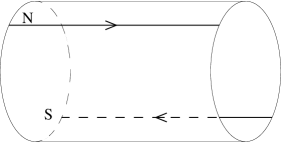
Figure 1: Timelike Wilson line.

The insertions ${\cal O}(t_{i},{\bf n}_{i})$ are some local operators. This expression can be interpreted as a transition amplitude in the Yang-Mills theory on $S^{3}$ with the external quark and antiquark sitting at the south and the north pole of the $S^{3}$. At $t=-\infty$ we have a ground state of the Yang-Mills on $S^{3}$ with two sources which preserves $1\over 2$ of the supersymmetry. At $t=t_{i}$ we act by the operators ${\cal O}(t_{i},{\bf n}_{i})$ and then we compute the overlap of the resulting state with the ground state at $t=+\infty$.

Besides inserting the local operators ${\cal O}(t_{i},{\bf n}_{i})$ we can perturb the ground state by moving the external source. Let us deform the contour $C$ as shown on Fig.2. We leave the component at the south pole unchanged, and we create the ”wiggle” near the north pole:

$${\bf n}(t)=\left(\sqrt{1-\vec{x}^{\;2}(t)},\;x_{1}(t),x_{2}(t),x_{3}(t)\right)$$ (3)

where $x_{1}(t),x_{2}(t),x_{3}(t)$ are all zero outside the small interval $-a<t<a$. This corresponds to the accelerated motion of one of the external charges.

Figure 2: Moving one of the sources.

The moving charge emits radiation, therefore at $t>a$ the system is in some excited state. One can try to characterize this excited state and study its dependence on the trajectory of the charge. If this state can be described quasiclassically one can ask about the energy. The analogous question in classical electrodynamics is answered by the Liénard formula [15, 16]:

$$\Delta E=A\int_{-\infty}^{\infty}{\ddot{\vec{x}}^{\;2}-\left.[\dot{\vec{x}}\times\ddot{\vec{x}}]\right.^{2}\over(\,1-\dot{\vec{x}}^{\;2}\,)^{\scriptstyle 3\atop}}dt,$$ (4)

$$A={2\over 3}e^{2}$$

The functional form of this expression follows from the dimensional analysis and the relativistic invariance under the assumption that the emitted energy is a local functional of the particle trajectory. This assumption relies on the fact that the Maxwell equations are linear. Indeed, the field created by the particle at any given moment of its history is independent of the fields already created earlier; it just adds to them. Besides that, the electromagnetic field at any given point $P$ of space depends only on the trajectory of the particle near the intersection with the past light cone of $P$; therefore there is no interference between the electromagnetic waves created at different times.

The Yang-Mills theory is nonlinear, therefore we might expect that the energy emitted by the moving source is a nonlocal functional of the trajectory. At strong coupling we can study this process using the AdS/CFT correspondence. The theory with two external quarks corresponds to the supergravity in $AdS_{5}\times S^{5}$ with the classical string with two boundaries. At $t<-a$ the worldvolume of the string is $AdS_{2}\subset AdS_{5}$ with the Lorentzian signature. The movement of the source at $t\in[-a,a]$ results in the nonlinear wave on the string worldsheet. In the large $N$ limit we neglect the interaction with the closed strings. Therefore all the energy on the string theory side is in this nonlinear wave. We will find the corresponding exact solution and compute its energy. The answer is given by the Liénard formula (4) with the overall coefficient

$$A={\sqrt{\lambda}\over 2\pi}$$ (5)

It is surprising that the radiated energy is a local functional of the trajectory in the strongly coupled Yang-Mills theory which is highly nonlinear. This is a manifestation of the integrability of the classical worldsheet sigma model [17, 18]. It would be interesting to see if the quantum sigma model has an analogous property.

The plan of the paper. In Section 2 we study the waves on the string worldsheet in the linearized approximation. In Section 3 we introduce the solution for the nonlinear wave and discuss its basic properties. In Section 4 we compute the energy and the momentum carried by the wave. In Section 5 we discuss open questions.

2 Linearized equations.

2.1 Two straight lines.

In this section we will consider the string worldsheet corresponding to the quark-antiquark pair, and study its small fluctuations. $AdS_{5}$ is the universal covering space of the hyperboloid

$$X_{-1}^{2}+X_{0}^{2}-X_{1}^{2}-X_{2}^{2}-X_{3}^{2}-X_{4}^{2}=1$$ (6)

in ${\bf R}^{2+4}$. We can parametrize this hyperboloid by $\rho,t,{\bf n}$: $X_{-1}+iX_{0}=e^{it}\cosh\rho$, $X_{a}=n_{a}\sinh\rho,a=1,2,3,4$. The boundary is at $\rho=\infty$, it is a product of $S^{1}$ parametrized by $t$ and $S^{3}$ parametrized by $\bf n$. We will consider the string worldsheet with two boundaries. One boundary has ${\bf n}=(0,0,0,1)$ and $t$ going from $-\infty$ to $+\infty$ and the other has ${\bf n}=(0,0,0,-1)$ and $t$ goes from $+\infty$ to $-\infty$. The corresponding worldsheet is given by the equation:

$$X_{1}=X_{2}=X_{3}=0$$ (7)

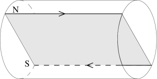
Figure 3: $AdS_{2}\subset AdS_{5}$

It may be parametrized by $X_{-1}$, $X_{0}$ and $X_{1}$ satisfying $X_{-1}^{2}+X_{0}^{2}-X_{1}^{2}=1$. The induced metric makes it $AdS_{1+1}$. The Poincare coordinates cover a wedge of the AdS space:

$$v= (X_{-1},X_{0},X_{1},X_{2},X_{3},X_{4})=$$ (9)

$$=\left[{1-x_{\mu}^{2}+h^{2}\over 2h},{x_{0}\over h};{\vec{x}\over h},{1+x_{\mu}^{2}-h^{2}\over 2h}\right]$$

The trajectory of the quark on the south pole is not covered at all by these coordinates. A part of the trajectory of the northern quark is covered, and is given by the equations: $x_{1}=x_{2}=x_{3}=0$. The trajectory is a straight line. The string worldsheet is the upper half-plane ending on this straight line.

2.2 Small fluctuations.

The Poincare coordinates are convenient for studying the linearized wave equations on the worldsheet. We will describe the wave by the displacement $x_{i}(x_{0},h)$. The variation of the area functional is:

$$S=\int{dx_{0}dh\over h^{2}}\left[\left({\partial x_{i}\over\partial x_{0}}\right)^{2}-\left({\partial x_{i}\over\partial h}\right)^{2}\right]$$ (10)

The wave equation for $x_{i}$ is:

$${\partial^{2}x_{i}\over\partial x_{0}^{2}}-{\partial^{2}x_{i}\over\partial h^{2}}+{2\over h}{\partial x_{i}\over\partial h}=0$$ (11)

It follows that $y_{i}={1\over h}{\partial x_{i}\over\partial h}$ is a harmonic function: $y_{i}=-x_{i+}^{\prime\prime}(x_{0}+h)-x_{i-}^{\prime\prime}(x_{0}-h)$. Therefore

$$x_{i}(x_{0},h)=-hx_{i+}^{\prime}(x_{0}+h)+hx_{i-}^{\prime}(x_{0}-h)+x_{i+}(x_{0}+h)+x_{i-}(x_{0}-h)$$ (12)

Notice that $x_{i}(x_{0},0)=x_{i+}(x_{0})+x_{i-}(x_{0})$ and $\left.{\partial^{3}\over\partial h^{3}}\right|_{h=0}x_{i}(x_{0},h)=-2x_{+}^{\prime\prime\prime}(x_{0})+2x_{-}^{\prime\prime\prime}(x_{0})$. Therefore the shape of the minimal surface is uniquely determined by the shape of the boundary and the third derivative at the boundary (see also Section 6 of [19]).

The solution (12) can be thought of as a sum of the left-moving wave parametrized by $x_{i+}$ and the right-moving wave parametrized by $x_{i-}$. Suppose that the quark was at rest for the times $x_{0}<0$, then moved a little bit at $0<x_{0}<a$ and then returned to its original position and stayed at rest for $x_{0}>a$. Such a motion will create a right-moving wave, and the left-moving part will be zero (that is, $x_{i+}=0$). The fluctuation of the worldsheet will be localized in the strip $x_{0}-h\in[0,a]$. If we stay in the Poincare patch we would see only a part of the story. Let us follow the wave beyond the Poincare patch. The hyperboloid is covered by the two copies of the Poincare patches which we will denote ${\cal P}_{0}$ and ${\cal P}_{1}$. In the parametrization (9) ${\cal P}_{0}$ covers the region $h>0$ and ${\cal P}_{1}$ covers $h<0$. The wave is localized in a strip $x_{0}-h\in[0,a]$. In this strip the coordinates $u=h^{-1}$ and $v=x_{0}-h$ are nonsingular. We can continue the solution beyond the Poincare patch by relaxing the condition $u>0$ and considering arbitrary $u$.

Figure 4: A right-moving wave.

This gives a left-moving wave in the second Poincare patch ${\cal P}_{1}$. The full solution in the hyperboloid is:

$$\begin{array}[]{l}x_{i}(x_{0},h)=hx^{\prime}_{i}(x_{0}-h)+x_{i}(x_{0}-h)\;\;\;{\rm in}\;\;\;{\cal P}_{0}\\[5.0pt] x_{i}(x_{0},h)=-hx^{\prime}_{i}(x_{0}+h)+x_{i}(x_{0}+h)\;\;\;{\rm in}\;\;\;{\cal P}_{1}\end{array}$$ (13)

The boundary condition in ${\cal P}_{1}$ is the same as it was in ${\cal P}_{0}$. The solution (13) has the following physical meaning. We create a wave on the string worldsheet by the small motion $\delta x_{i}(x_{0})$ of one of the boundaries at time $x_{0}=0$. The wave propagates forward in time and reaches the second boundary where it is totally absorbed by the identical motion $\delta x_{i}(x_{0})$ of the second boundary (see Figure 4).

In order to better understand this solution it is useful to remember a simple geometric feature of the boundary ${\bf R}\times S^{3}$. The geometry of ${\bf R}\times S^{3}$ and the propagation of the massless fields on ${\bf R}\times S^{3}$ was considered in great detail in [20]. Given a point $P\in{\bf R}\times S^{3}$ let us consider the future light cone of $P$. Because of the symmetries of $S^{3}$, the light rays emitted at point $P$ will refocus and converge at some other point $P^{\prime}\in{\bf R}\times S^{3}$. The correspondence $P\mapsto P^{\prime}$ is a symmetry of ${\bf R}\times S^{3}$, which is denoted $Z$ in [20]. It is a combination of the reflection ${\bf n}\to-{\bf n}$ of $S^{3}$ and the shift $t\to t+\pi$ in ${\bf R}$ (we choose the radius of $S^{3}$ to be $1$). In these notations our wave is generated by the small perturbation $\delta x_{i}$ of the boundary at the point $P$ with the coordinates $x_{\mu}=0$, propagates with the speed of light forward in time and is then totally absorbed by the identical perturbation $\delta x_{i}$ of the second boundary at the point $P^{\prime}=Z.P$. If we do not perturb the second boundary at $P^{\prime}$ then the wave will not get absorbed. Instead it will reflect from the second boundary and travel back towards to the first boundary. To describe the corresponding solution we have to consider the right moving wave generated by the perturbation $-\delta x_{i}$ at the point $P^{\prime}$, and add it to the solution (13). This solution corresponds to the wave created by the perturbation $\delta x_{i}$ at $P$, then traveling with the speed of light towards the second boundary, then being reflected from the second boundary near the point $P^{\prime}=Z.P$, then coming back to the first boundary and being cancelled there by the perturbation $-\delta x_{i}$ at the point $P^{\prime\prime}=Z^{2}.P$. Of course, we could also add a right moving wave generated by $\delta x_{i}$ at $P^{\prime\prime}$, and get a reflected wave again.

Let us summarize our discussion of the linear waves. The small perturbation $\delta x_{i}$ of the boundary at the point $P$ will create a wave moving forward in time with the speed of light, bouncing back and forth between the two boundaries. We can absorb this wave by the perturbation $\delta x_{i}$ at some point $Z^{2n+1}.P$, or by the perturbation $-\delta x_{i}$ at some point $Z^{2n}.P$ — see Figure 5.

Figure 5: A linear wave.

3 Nonlinear wave.

In this section we will construct the extremal surface corresponding to the solution (13) for a finite perturbation. It is a nonlinear wave on the worldsheet emitted at some point $P$ of the boundary and absorbed at the point $Z.P$.

The construction. Let us realize the AdS space as a hyperboloid in ${\bf R}^{2+4}$ consisting of the vectors $v\in{\bf R}^{2+4}$ satisfying $||v||^{2}=1$. The AdS space is actually a universal covering space of this hyperboloid. But our solution all fits in a simply-connected domain of the hyperboloid and therefore it is not important for our purposes to distinguish between the hyperboloid and its universal covering. The boundary consist of the light rays in ${\bf R}^{2+4}$. Suppose that $l(\tau)$ is a one-parameter family of the lightlike vectors representing the boundary of the string worldsheet. We will choose the parameter $\tau$ so that $\left({dl\over d\tau},{dl\over d\tau}\right)=1$. Consider the following two-dimensional surface parametrized by the two real parameters $\tau$ and $\sigma$:

$$v(\tau,\sigma)=-\dot{l}(\tau)+\sigma l(\tau)$$ (14)

Let us prove that this surface is extremal. Indeed, let us start with computing the induced metric:

$$ds^{2}=||dv(\tau,\sigma)||^{2}=(||\ddot{l}||^{2}+\sigma^{2})d\tau^{2}+2d\tau d\sigma$$ (15)

The area is therefore just $\int d\tau d\sigma$. We have to prove that the area does not change under the infinitesimal variations of the surface. We can describe the infinitesimal variations by the normal vector field $\xi(\tau,\sigma)$. We should have $(\xi,-\dot{l}+\sigma l)=0$ (because $\xi$ is tangent to the hyperboloid) and also $(\xi,l)=0$ and $(\xi,-\ddot{l}+\sigma\dot{l})=0$ (because $\xi$ is normal to the surface). It follows that $(\xi,l)=(\xi,\dot{l})=(\xi,\ddot{l})=0$. The metric on the perturbed surface is, to the first order in $\xi$:

$$ds^{2}=||dv(\tau,\sigma)||^{2}=\left(||\ddot{l}||^{2}+\sigma^{2}+2\left(\xi,{d^{3}l\over d\tau^{3}}\right)\right)d\tau^{2}+2d\tau d\sigma+o(\xi)$$ (16)

Therefore the variation of the area functional is zero.

The regularized area of this surface is zero. Indeed, let us regularize the area functional by restricting the $\sigma$ coordinate to run from $-S$ to $S$. According to the prescription in [1, 2, 5] the regularized area is the area minus the length of the boundary. The area is $2S\int d\tau$ and the length of the boundary is $2\int d\tau\sqrt{S^{2}+||\ddot{l}||^{2}}$. Therefore the area is cancelled by the length of the boundary in the limit when $S$ is large.

Let us rewrite (14) in the Poincare coordinates:

$$\begin{array}[]{l}h(\tau,\sigma)=\sigma^{-1}\\[5.0pt] x_{\mu}(\tau,\sigma)=\sigma^{-1}\dot{x}_{\mu}(\tau)+x_{\mu}(\tau)\end{array}$$ (17)

Here we have assumed that $\dot{x}_{\mu}\dot{x}^{\mu}=1$. This is a right moving wave. The left moving wave is

$$\begin{array}[]{l}h(\tau,\sigma)=\sigma^{-1}\\[5.0pt] x_{\mu}(\tau,\sigma)=-\sigma^{-1}\dot{x}_{\mu}(\tau)+x_{\mu}(\tau)\end{array}$$ (18)

The left moving wave in the global coordinates: $v(\tau,\sigma)=\dot{l}(\tau)+\sigma l(\tau)$.

The solution may have wedges. Suppose that the second derivative $\ddot{x}$ of the boundary contour is not continuous. Then the resulting wave is not smooth. The light ray originating from the point where $\ddot{x}$ has a jump is a ”wedge” on the worldsheet; the first derivative of the embedding jumps across the wedge. In general, the Lorentzian extremal surfaces may have wedges. The wedge does not have to be a null-geodesic in AdS, but it has to be a lightlike curve. Indeed, let us consider a surface composed of two smooth extremal surfaces glued along the lightlike curve. We claim that this surface is extremal. Let us introduce on both surfaces the coordinates $x_{+},x_{-}$ so that they agree on the intersection and the induced metric is $f(x_{+},x_{-})dx_{+}dx_{-}$. Consider the variation of the area under the infinitesimal deformation $\delta X^{\mu}(x_{+},x_{-})=\xi^{\mu}(x_{+},x_{-})$. Because each of the two surfaces are extremal, the possible change in the area comes from the boundary term which has a form

$$\int_{L}dx_{+}\xi_{\mu}{\partial\over\partial x_{+}}X^{\mu}$$

where the integral is over the intersection. But $X^{\mu}$ is continuous across the intersection, therefore ${\partial\over\partial x_{+}}X^{\mu}$ is also continuous. Therefore the boundary terms from for the two surfaces cancel each other.

A change in boundary conditions. The nonlinear wave which we have constructed propagates from one boundary to the other. Both boundaries are perturbed. What happens if we perturb only one boundary, leaving the other one a straight line? Infinitesimal perturbation will create a wave localized in a strip, which bounces forever back and forth between the boundaries — see Figure 5. What can we say about the solution of the nonlinear equations? We know that a part of the worldsheet has the same shape as the right-moving wave.

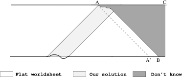
Figure 6: Changing the boundary conditions on the upper boundary.

The solution is scetched on Figure 6. The curve $AB$ is a light ray. We know the solution on the left of $AB$. Indeed, the boundary condition on the upper boundary is different from the boundary condition for our solution (14) only on the halfline $AC$. The difference can only affect the solution in the future of this halfline, which is the dark area of Figure 6.

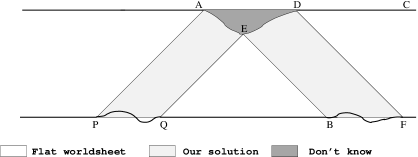
Figure 7: Reflection of nonlinear wave.

There is an additional qualitative argument which implies that most of the solution in the dark area is actually a left moving wave, see Figure 7. The boundary conditions at the upper boundary leave undefined the third derivative $\alpha^{i}={\partial^{3}x^{i}\over\partial h^{3}}$ (see for example [19]). To the left of the point $A$ the worldsheet is flat. Therefore we should take $\alpha^{i}=0$ to the left of $A$. To the right of A let us adjust this third derivative in such a way that the resulting minimal surface contains the interval $AE$ of the light ray. The resulting surface will also contain an interval $ED$ of some other light ray. Now, let us continue the solution below the null curve $AED$ as shown on Figure 7: three flat regions and two waves, one right-moving and one left-moving. We do not have a problem adding the left-moving nonlinear wave and the right-moving nonlinear wave because they do not overlap. The only ”dark” region where we do not know the solution is the triangle $AED$. We need to know the solution in this region if we want to learn the relation between the trajectory of the source between points $P$ and $Q$ and the trajectory between the points $B$ and $F$.

Scattering. Similar arguments can be applied to the scattering of the right moving wave on the left moving wave — see Figure 8. The left moving wave collides with the right moving wave at some point $B$. We know the solution for the nonlinear wave, therefore we know the shape of the null intervals $BA$ and $BC$. In principle one can find using the methods of [21] the shape of the worldsheet inside the diamond $ABCD$. The intervals $AB$, $BC$, $CD$ and $DA$ are all null curves. One should then adjust the trajectory of the source in the intervals $XY$ and $ZW$ so that the left- and right-moving waves created by the source contain null intervals $AD$ and $DC$.

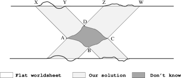
Figure 8: Scattering

It may happen that the light rays $YD$ and $ZD$ do not belong to the same vertical ($\vec{x}=0$ in Poincare coordinates) plane. In this case the interval $YZ$ has to be a part of a hyperbola, rather than a straight line.

When the left moving wave passes through the right moving wave, the shapes of both waves are distorted. A simple way to see it is to look at the propagation of the left moving light rays in the background of the right moving nonlinear wave. One can see that the image of the boundary is distorted after the light rays pass through the right-moving nonlinear wave. This means that even a linear left-moving wave is generally distorted by the nonlinear wave.

4 Energy of the wave.

We will compute the energy of the wave in the Poincare coordinates, with respect to the time $x^{0}$ defined in the Poincare patch. Let us parametrize the worldsheet by $T=x_{0}$ and $h$. The energy is

$$E={\sqrt{\lambda}\over 2\pi}\int_{0}^{\infty}{dh\over h^{2}}{1+\left({\partial\vec{x}\over\partial h}\right)^{2}\over\sqrt{1-\left({\partial\vec{x}\over\partial T}\right)^{2}+\left({\partial\vec{x}\over\partial h}\right)^{2}-\left({\partial\vec{x}\over\partial T}\right)^{2}\left({\partial\vec{x}\over\partial h}\right)^{2}+\left({\partial\vec{x}\over\partial T}\cdot{\partial\vec{x}\over\partial h}\right)^{2}}}$$ (19)

To compute this integral on our solution it is useful to change the coordinates from $(T,h)$ to $(T,t)$ (see Figure 9):

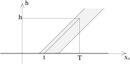
Figure 9: Notations for the calculation of the energy.

$$h(T,t)=(T-t)\sqrt{1-\left({d\vec{x}(t)\over dt}\right)^{2}}$$ (20)

where $\vec{x}(t)$ is the trajectory of the endpoint of the string. In these coordinates

$$\vec{x}(T,t)=\vec{x}(t)+(T-t){d\vec{x}(t)\over dt}$$ (21)

A straightforward calculation gives:

$$\left.{\partial\vec{x}\over\partial T}\right|_{h}=\vec{v}+(T-t){1-\vec{v}^{2}\over 1-\vec{v}^{2}+(T-t)(\vec{v}\cdot\vec{a})}\;\vec{a}$$ (22)

$$\left.{\partial\vec{x}\over\partial h}\right|_{T}=-(T-t){\sqrt{1-\vec{v}^{2}}\over 1-\vec{v}^{2}+(T-t)(\vec{v}\cdot\vec{a})}\vec{a}$$ (23)

Substituting $\left.{\partial\vec{x}\over\partial T}\right|_{h}$ and $\left.{\partial\vec{x}\over\partial h}\right|_{T}$ into (19) and discarding a total derivative we get:

$$E={\sqrt{\lambda}\over 2\pi}\int dt{\ddot{\vec{x}}^{\;2}-\left.[\dot{\vec{x}}\times\ddot{\vec{x}}]\right.^{2}\over(\,1-\dot{\vec{x}}^{\;2}\,)^{\scriptstyle 3\atop}}$$ (24)

This expression has the same form as the Liénard formula for the energy emitted by the moving charge in the classical electrodynamics [15, 16]. One can also compute the momentum:

$$\vec{P}={\sqrt{\lambda}\over 2\pi}\int_{0}^{\infty}{dh\over h^{2}}{{\partial\vec{x}\over\partial T}+\left({\partial\vec{x}\over\partial h}\right)^{2}{\partial\vec{x}\over\partial T}-\left({\partial\vec{x}\over\partial T}\cdot{\partial\vec{x}\over\partial h}\right){\partial\vec{x}\over\partial h}\over\sqrt{1-\left({\partial\vec{x}\over\partial T}\right)^{2}+\left({\partial\vec{x}\over\partial h}\right)^{2}-\left({\partial\vec{x}\over\partial T}\right)^{2}\left({\partial\vec{x}\over\partial h}\right)^{2}+\left({\partial\vec{x}\over\partial T}\cdot{\partial\vec{x}\over\partial h}\right)^{2}}}$$ (25)

$$={\sqrt{\lambda}\over 2\pi}\int dt{\ddot{\vec{x}}^{\;2}-\left.[\dot{\vec{x}}\times\ddot{\vec{x}}]\right.^{2}\over(\,1-\dot{\vec{x}}^{\;2}\,)^{\scriptstyle 3\atop}}\dot{\vec{x}}$$ (26)

This expression actually follows from (24) and the Lorentz invariance. The relativistic formula is $P^{\mu}={\sqrt{\lambda}\over 2\pi}\int{d^{2}x_{\sigma}\over ds^{2}}{d^{2}x^{\sigma}\over ds^{2}}dx^{\mu}$ where $s$ is a proper time.

5 Discussion.

We have studied the nonlinear waves which are excitations of the extremal surface $AdS_{2}\subset AdS_{5}$. In some sense all the extremal surfaces in $AdS_{5}$ which are sufficiently close to $AdS_{2}$ can be obtained as ”nonlinear superpositions” of these waves. Is it possible to give a similar description of the extremal surfaces extending in $S^{5}$? Perhaps they can be obtained as excitations of the supersymmetric extremal surfaces introduced in [22].

It would be very interesting to understand the role of these nonlinear waves in the quantum worldsheet theory [18]. If the quantum CFT is integrable, then one should probably expect that the radiated energy is a local functional of the trajectory in the large $N$ theory at finite $\lambda$. This raises the possibility of a check by a perturbative field theory computation. Actually at finite $\lambda$ one cannot literally ask the question about the radiated energy. The emitted radiation will be in some quantum state which does not necessarily have a definite energy. But one can ask for example about the total probability of emitting a quant of radiation.

We hope to return to these questions in a future publication.

References

- [1] S.J. Rey, J.T. Yee, ”Macroscopic strings as heavy quarks: Large-N gauge theory and anti-de Sitter supergravity”, Eur.Phys.J. C22 (2001) 379-394, hep-th/9803001.
- [2] J.M. Maldacena, ”Wilson loops in large N field theories”, Phys.Rev.Lett. 80 (1998) 4859-4862, hep-th/9803002.
- [3] S.J. Rey, S. Theisen, J.T. Yee, ”Wilson-Polyakov Loop at Finite Temperature in Large N Gauge Theory and Anti-de Sitter Supergravity”, Nucl.Phys. B527 (1998) 171-186, hep-th/9803135.
- [4] D. Berenstein, R. Corrado, W. Fischler, J. Maldacena, ”The Operator Product Expansion for Wilson Loops and Surfaces in the Large N Limit”, Phys.Rev. D59 (1999) 105023, hep-th/9809188
- [5] N. Drukker, D.J. Gross, H. Ooguri, ”Wilson Loops and Minimal Surfaces”, Phys.Rev. D60 (1999) 125006, hep-th/9904191.
- [6] J.K. Erickson, G.W. Semenoff, K. Zarembo, ”Wilson Loops in N=4 Supersymmetric Yang–Mills Theory”, Nucl.Phys. B582 (2000) 155-175, hep-th/0003055.
- [7] N. Drukker, D.J. Gross, ”An Exact Prediction of N=4 SUSYM Theory for String Theory”, J.Math.Phys. 42 (2001) 2896-2914, hep-th/0010274.
- [8] M. Rho, S.-J. Sin, I. Zahed, ”Elastic Parton-Parton Scattering from AdS/CFT”, Phys.Lett. B466 (1999) 199-205, hep-th/9907126.
- [9] R.A. Janik, R. Peschanski, ”Minimal surfaces and Reggeization in the AdS/CFT correspondence”, Nucl.Phys. B586 (2000) 163-182, hep-th/0003059; ”Reggeon exchange from AdS/CFT”, Nucl.Phys. B625 (2002) 279-294, hep-th/0110024; R.A. Janik, ”String Fluctuations, AdS/CFT and the Soft Pomeron Intercept”, Phys.Lett. B500 (2001) 118-124, hep-th/0010069
- [10] S. S. Gubser, I. R. Klebanov, A. M. Polyakov, ”A semi-classical limit of the gauge/string correspondence”, hep-th/0204051, Nucl.Phys. B636 (2002) 99-114.
- [11] M. Kruczenski, ”A note on twist two operators in N=4 SYM and Wilson loops in Minkowski signature”, hep-th/0210115.
- [12] Yu. Makeenko, ”Light-Cone Wilson Loops and the String/Gauge Correspondence”, hep-th/0210256.
- [13] A. V. Belitsky, A. S. Gorsky, G. P. Korchemsky, ”Gauge/string duality for QCD conformal operators”, hep-th/0304028.
- [14] V. Pestun, K. Zarembo, ”Comparing strings in AdS(5)xS(5) to planar diagrams: an example”, Phys.Rev. D67 (2003) 086007, hep-th/0212296.
- [15] L.D. Landau, E.M. Lifshitz, ”The Classical Theory of Fields”, Pergamon Press, 1975.
- [16] J.D. Jackson, ”Classical Electrodynamics”, John Wiley & Sons, Inc., 1975.
- [17] G. Mandal, N.V. Suryanarayana, S.R. Wadia, ”Aspects of Semiclassical Strings in AdS5”, Phys.Lett. B543 (2002) 81-88, hep-th/0206103.
- [18] I. Bena, J. Polchinski, R. Roiban, ”Hidden Symmetries of the Superstring”, hep-th/0305116.
- [19] A. Mikhailov, ”Special contact Wilson loops”, hep-th/0211229.
- [20] M. Lüscher, G. Mack, ”Global conformal invariance in quantum field theory”, Comm. Math. Phys. 41 (1975), 203–234.
- [21] L.D. Faddeev, L.A. Takhtajan, ”Hamiltonian methods in the theory of solitons”, Springer-Verlag, Berlin, 1987.
- [22] K. Zarembo, ”Supersymmetric Wilson loops”, Nucl.Phys. B643 (2002) 157-171, hep-th/0205160.