Dressing up the kink

Abstract

Many quantum field theoretical models possess non-trivial solutions which are stable for topological reasons. We construct a self-consistent example for a self-interacting scalar field–the quantum (or dressed) kink–using a two particle irreducible effective action in the Hartree approximation. This new solution includes quantum fluctuations determined self-consistently and nonperturbatively at the 1-loop resummed level and allowed to backreact on the classical mean-field profile. This dressed kink is static under the familiar Hartree equations for the time evolution of quantum fields. Because the quantum fluctuation spectrum is lower lying in the presence of the defect, the quantum kink has a lower rest energy than its classical counterpart. However its energy is higher than well-known strict 1-loop results, where backreaction and fluctuation self-interactions are omitted. We also show that the quantum kink exists at finite temperature and that its profile broadens as temperature is increased until it eventually disappears.

Topological defects are perhaps the best known nonlinear solutions of quantum field theories. They are explicitly spatially inhomogeneous yet localized and have finite energy configurations (sometimes involving defect-antidefect pairs) Rajaraman ; Vilenkin . Moreover topological defects, particularly extended ones (strings, domain walls), have configurational entropies that increase exponentially with their size. For these reasons defects are important vehicles of disorder. They can lead to phase transitions not predictable in their absence, such as Kosterlitz-Thouless Kadanoff , or become the mesoscopic traces of high energy disorder, as happens in defect formation under sudden quenches. Defects can also lead to nonperturbative screening effects, e.g. of static magnetic fields by ’t-Hooft-Polyakov monopoles Polyakov .

Because defects are localized solutions carrying quantized topological numbers they can often be thought of as generalized quantum particles. In fact in certain circumstances topological solutions dominate the phenomenology and should then be thought as the fundamental excitations of a new (often more tractable) model, related to the original by a duality transformation. Such changes of perspective have been the source of valuable insights into the nonperturbative properties of models of condensed matter, high-energy particle physics and quantum gravity.

While the existence and stability of topological solutions follows from general considerations about the symmetries and dimensionality Kibble of a given model, the detailed properties of topological solutions, e.g. their size and energy, depend on the back-reaction from the background of quantum (and thermal) fluctuations in which they live. For example the difference in energy between the dressed defect and its classical counterpart will affect estimates for the probability of its spontaneous nucleation via quantum or thermal fluctuations LytheHabib . The same rest energy shift also affects the defect’s dynamical response. Only a self-consistent treatment, where mass corrections occur to all orders in the loop expansion $\hbar\lambda$ can begin to probe the motion at non-zero momentum and long times BB1 . In some cases fluctuations may even stabilize nontopological classical field profiles Jaffe , but it is not known whether 1-loop results survive a self-consistent treatment.

Incorporating the effects of fluctuations is technically quite difficult, which explains in part why most previous work has relied on a strict loop expansion, neglecting either backreaction on the classical mean-field profile or self-coupling of the fluctuation degrees of freedom. For example, calculations carried out to 2-loop order appear in Ref. 2loop , and a variational self-consistent calculation without backreaction on the mean field is performed in Ref. Boyanovsky . Since the corresponding “solutions” are not self-consistent, in particular they will not be static under non-equilibrium quantum field evolutions non-eq . Fermionic backreaction has been considered in the calculation of the sphaleron energy, which is relevant for estimating baryon number violation Moore ; Schroers . This computation showed the sphaleron energy to be quite insensitive to such corrections, however quartic self-couplings of the scalar field were neglected Schroers . It is precisely these nonlinear field selfinteractions which we wish to consider here.

To start addressing the above issues we construct here an example of a self-consistent quantum topological defect. For simplicity, and for the benefit of analytical cross-checks on our numerical results at both the classical and 1-loop quantum levels, we analyze the familiar $\phi^{4}$ kink in 1+1 dimensions. There has also been a lattice Monte Carlo study of the quantum kink Ardekani , providing a benchmark against which we can measure the efficacy of the self-consistent Hartree approximation. The methods developed here promptly generalize to other cases. Self-consistent spherically symmetric droplets, in particular, will be discussed elsewhere scbounce . We include quantum effects at the 1-loop resummed level with backreaction on the mean field by applying the familiar Hartree approximation to a $2PI$ effective action 2PI . This technique places the two-point correlation function on the same level as the one-point function, or mean field, thus backreaction is included as naturally as the nonperturbative resummation of fluctuations. At this level of approximation, we obtain a local, nonlinear eigenvalue-type equation for the quantum fluctuations. The next level of improvement, at 2-loop resummed, would lead to a nonlocal integro-differential problem, which would require methods of solution different from the ones developed below. Specifically we take the $\lambda\phi^{4}$ model with potential

$$V(\phi)=\frac{\lambda}{4}\left(\phi^{2}-\frac{\mu^{2}}{\lambda}\right)^{2}.$$ (1)

Then the classical kink solution has the well known analytical form

$$\phi(x)=\frac{\mu}{\sqrt{\lambda}}\tanh\left(\frac{\mu}{\sqrt{2}}x\right).$$ (2)

To set up the quantum problem we separate, as usual, the quantum field into a mean $\varphi\equiv\langle\phi\rangle$ and a fluctuation operator-valued field $\hat{\psi}$ ($\langle\hat{\psi}\rangle=0$), such that $\phi(x,t)=\varphi(x,t)+\hat{\psi}(x,t)$. The Hartree (or 1-loop resummed) equations for the mean field and the connected (Wightman) two-point function $G(x,t;x^{\prime},t^{\prime})=\langle\hat{\psi}(x,t)\psi(x^{\prime},t^{\prime})\rangle$ then become

$$\left[\Box-\mu^{2}+\lambda\varphi^{2}(x,t)+3\lambda G(x,t)\right]\varphi(x,t)=0,$$ (3)

$$\left[\Box+\chi(x,t)\right]G(x,t;x^{\prime},t^{\prime})=0,$$ (4)

$$\chi(x,t)=-\mu^{2}+3\lambda\varphi^{2}(x,t)+3\lambda G(x,t),$$ (5)

with $\Box=\partial_{t}^{2}-\partial_{x}^{2}$ and $G(x,t)\equiv G(x=x^{\prime},t=t^{\prime})$. We seek a static solution to equations (3-5), obeying boundary conditions $\varphi(x\rightarrow+\infty)=-\varphi(x\rightarrow-\infty)=\varphi_{0}$, where $\varphi_{0}$ is one of the degenerate vacuum expectation values of the quantum field. These boundary conditions imply that the mean field must cross zero at some $x_{0}$, which defines the center of the kink.

Eqs. (4-5) can be converted into a (non-linear) eigenvalue problem by the familiar procedure of decomposing $G(x,t;x^{\prime},t^{\prime})$ in a complete orthonormal basis of mode fields, which we shall denote by $\{\psi_{k}(x,t)\}$. The procedure has been detailed extensively elsewhere non-eq , and we do not repeat it here. The result is

$$G(x,t;x^{\prime},t^{\prime})=\sum_{k}\left\{(N(k)+1)\psi_{k}(x,t)\psi_{k}^{*}(x^{\prime},t^{\prime})+N(k)\psi_{k}^{*}(x,t)\psi_{k}(x^{\prime},t^{\prime})\right\},$$ (6)

where $N(k)$ is occupation number in this basis, which becomes the Bose-Einstein distribution $n_{B}(k)$, if the system is in thermal equilibrium $N(k)\rightarrow n_{B}(k)=\left(e^{\hbar\omega_{k}/T}-1\right)^{-1}$, with $\omega_{k}$ the energy eigenvalue associated with the eigenvector $\psi_{k}(x,t)$. In particular, the equal-point function acquires the very simple form

$$G(x,t)=\sum_{k}\left[2N(k)+1\right]\psi_{k}(x,t)\psi_{k}^{*}(x,t).$$ (7)

Next we specify a basis $\left\{\psi_{k}(x,t)\right\}$, together with the scalar product

$$\left(\psi_{k}(x,t).\psi_{q}(x,t)\right)=i\int dx\left\{\psi_{k}^{*}(x,t)\partial_{t}\psi_{q}(x,t)-\psi_{q}(x,t)\partial_{t}\psi_{k}^{*}(x,t)\right\}.$$ (8)

Because we seek a static solution the self-consistent $\chi(x)$ is time independent. Then each $\psi_{k}(x,t)$ can be separated into the product of functions of time and space as

$$\psi_{k}(x,t)=\sqrt{\frac{\hbar}{2\omega_{k}}}e^{-i\omega_{k}t}g_{k}(x),$$ (9)

and the inner product (8) can be written in terms of the $g_{k}(x)$ as

$$\left(g_{k}(x).g_{q}(x)\right)=\int dx~{}g_{k}^{*}(x)g_{q}(x),$$ (10)

which is familiar from quantum mechanics. With these definitions orthogonality in $\{g_{k}\}$ is equivalent to orthogonality in $\{\psi_{k}\}$. Moreover the completeness relation

$$\sum_{k}g_{k}(x)g_{k}^{*}(x^{\prime})=\delta^{D}(x-x^{\prime}),$$ (11)

must be satisfied as a result of the canonical equal-time commutation relations obeyed by the original quantum field. Finally the explicit self-consistent eigenvalue problem reads

$$\left[-\nabla_{x}^{2}+\chi(x)\right]g_{k}(x)=\omega_{k}^{2}g_{k}(x),$$ (12)

with the eigenmodes obeying periodic boundary conditions in the volume $x\in\left\{-L,L\right\}$: $g_{k}(L)=g_{k}(-L)$, and solved in conjunction with equation (3) for $\varphi$. In practice we discretize the fields on a spatial lattice of size $N$ and volume $L$. This provides a regularization of the quantum field theory. In addition we have to devise a renormalization scheme to render all results finite as the lattice spacing $a=L/N$ is taken to zero, i.e. in the continuum limit.

The 2-point function $G$, as defined in Eq. (7), contains an ultraviolet logarithmic divergence in the continuum limit. We specify the fluctuation physical mass and field expectation value over the trivial vacuum. These choices implicitly define the bare mass parameter $\mu^{2}$ as a function of the ultraviolet cutoff $\Lambda=\pi/a$ so as to absorb this divergence. Explicitly

$$\chi_{0}=2m^{2},\ \varphi^{2}_{0}=m^{2}/\lambda;\quad\rightarrow\quad\mu^{2}\equiv m^{2}+3\lambda G_{0},$$ (13)

$${\rm where}\quad G_{0}=\int_{-\Lambda}^{\Lambda}\frac{dk}{2\pi}\frac{\hbar}{2\sqrt{k^{2}+2m^{2}}}.$$ (14)

Substitution of $\mu^{2}$, hence defined, into expression (5) for $\chi(x)$ now leads to finite results, independent of $\Lambda$, as the continuum (and infinite volume limit) are taken.

The only remaining divergences occur in the calculation of the energy. The total energy can be split into a classical piece $E_{\rm cl}$ and the quantum (and thermal) fluctuation contribution $E_{\rm q}$. Taking expectation values we can write them as

$$E_{\rm q} =\int dx~{}\sum_{k}\left\{\psi_{k}(x)\left[-\nabla^{2}+\chi(x)\right]\psi(k)\right\}\left[1+2N(k)\right]-\frac{3}{4}\lambda G^{2}(x)$$ (15)

$$\equiv\delta m-\frac{3}{4}\lambda\int dx~{}G^{2}(x)+\sum_{n}\omega_{n}N(k_{n}),$$

$$E_{\rm cl} =\int dx~{}\left[\frac{(\nabla\varphi(x))^{2}}{2}+\frac{\lambda}{4}(\varphi^{2}-\mu^{2}/\lambda)^{2}\right].$$ (16)

The analysis of divergences is familiar at 1-loop, where it has been resolved in at least two distinct ways: by direct analysis of the divergences in a large momentum expansion Dashen ; Rajaraman and via the normal ordering of the fluctuation Hamiltonian operator, which is sufficient in 1+1 dimensions to extract the physical finite contribution Cahil ; BT ; Weidig . Because they are implemented very differently we have employed both methods as a check.

The most straightforward procedure, in our opinion, follows from direct analysis of the divergences in a large momentum expansion. For consistency we should start by substituting $\mu^{2}$ defined in (13) into (15-16), which eliminates all logarithmic divergences, up to an infinite constant. This constant results from the trace $\delta m=\sum_{n}\omega_{n}/2$. For large enough $n$, $\omega_{n}\rightarrow\omega^{0}_{n}=\sqrt{k_{n}^{2}+2m^{2}}\sim|k_{n}|$, resulting in a leading quadratic divergence. This divergence is also characteristic of the trivial vacuum energy and should be cancelled against it. With these prescriptions we can write the renormalized $E_{q}$ as

$$E_{q}^{R}=\frac{1}{2}\sum_{n}\left[\omega_{n}\left(1+2N(k)\right)-\omega^{0}_{n}\right]-\frac{1}{2}G_{0}\int dx\left[\chi(x)-\chi_{0}\right]-\frac{3}{4}\lambda\int dx\left[G(x)-G_{0}\right]^{2},$$ (17)

The classical energy piece $E_{\rm cl}$ is now to be evaluated as in (16), with the substitution $\mu^{2}\rightarrow m^{2}$.

Alternatively a finite energy expression for the trace in $\delta m$ can be constructed by suitably manipulating the fluctuation Hamiltonian operator. The normal ordered Hamiltonian is written in terms of a complete set of creation and annihilation operators in the kink background, which are then transformed via a Bogoliubov transformation to the trivial vacuum basis, where vacuum expectation values are computed. The residual contribution is finite and results from the existence of a non-zero particle number as seen back in the kink background mode basis. The final result is

$$\delta m=-\frac{1}{4}{\rm Tr}\left[\frac{({\cal O}-{\cal O}_{0})^{2}}{{\cal O}_{0}}\right],$$ (18)

where ${\cal O}=\left[-\partial_{x}^{2}+\chi(x)\right]$ and ${\cal O}_{0}={\cal O}$ with $\chi(x)=\chi_{0}$, corresponding to the trivial vacuum. The advantage of this procedure is that it is independent of the exact form of $\chi(x)$ in ${\cal O}_{k}$ and is thus equally valid at strict 1-loop order as well as in the resummed self-consistent approximation. In practice we cast this expression in the explicit form

$$\delta m=-\frac{1}{4}\sum_{i,j}|\left(g_{i}(x).g^{0}_{j}(x)\right)|^{2}\left[\frac{\omega^{2}_{i}}{\omega^{0}_{j}}-2\omega_{i}+\omega^{0}_{j}\right].$$ (19)

There remains a final ambiguity in expressions (17 - 19), namely the prescription of the upper (ultraviolet) cutoff in the mode sums. In the presence of a non-trivial background one expects a spectrum that contains a finite and discrete set of bound modes, lying below a continuum of scattering states. Physically it is the advent of these bound states that produces the leading (in magnitude) contribution to the energy shift of the quantum kink relative to the classical solution. Even for the lattice regularized theory, where the number of modes is finite and their eigenvalues discrete, there are at least two seemingly natural ways to choose the upper cutoff: including contributions up to a given mode number (say N), or alternatively, setting a cutoff in the magnitude of the eigenvalues. These two procedures lead in general to different results RvN . Fortunately the essence of this problem was analyzed in detail by Rebhan and van Nieuwenhuizen RvN , who showed that only a mode number cutoff leads to consistent results. By including all of the $N$ modes, bound and unbound, in our numerical treatment of these sums, we effectively implement this prescription without difficulty.

We are now left with the task of solving the interacting self-consistent problem numerically. We use a standard relaxation routine Nrecipes to solve Eq. (3), together with a set of LAPACK packages LAPACK to solve the real symmetric eigenvalue problem Eq.(4-5). At each step the fluctuation eigenproblem is solved to produce a new intermediate $G_{\rm int}(x)$, which we combine with the old value to produce a new trial $G_{\rm new}=(1-\gamma)G_{\rm old}+\gamma G_{\rm int}$, until convergence in $\varphi$ and $G(x)$ is reached, up to a specified precision. The adjustable parameter $0<\gamma<1$ controls the size of the update and can be adapted to optimize convergence.

Both mean-field and fluctuation update steps can be problematic and require some further discussion. The system retains an overall translational mode and iterative procedures where updates of $\varphi$ and $G$ are staggered can excite it, thus degrading convergence. To eliminate this problem we pin the kink’s center $x_{0}:\varphi(x_{0})=0$ to the mid-point of our spatial lattice. The full profile for the mean field is then obtained through the symmetry $\varphi(-(x-x_{0}))=-\varphi(x-x_{0})$. To strict 1-loop order there is a well-known fluctuation zero mode associated with the eigenvector $g_{0}(x)\sim\partial_{x}\phi$, regardless of the specific mean-field background. This follows immediately by taking a spatial derivative through the (classical) Eq. (3) and comparing the result to the 1-loop eigenvalue problem. This construction ceases to apply once fluctuations are made self-consistent, as their potential is shifted by a term $\sim 3\lambda G(x)$. Neglecting back-reaction on $\varphi(x)$ and assuming this effect to be small, knowledge of $G(x)$ allows us to estimate the energy shift of the former zero mode as $\omega^{2}_{0}\rightarrow 3\lambda\int dx~{}g^{*}_{0}(x)G(x)g_{0}(x)$, where $g_{0}(x)$ is the 1-loop zero mode eigenvector. This compares well with with our numerical results, even if $\lambda$ is not small. It predicts $\omega^{2}_{0}=0.513m^{2}$ vs. $\omega^{2}_{0}=0.504m^{2}$, with the parameters of Table 1, shown below. Thus we see that no fluctuation zero-mode persists in the self-consistent problem. We must nevertheless emphasize that the dressed kink retains an overall translational invariance at no energy cost (as the energy functional is independent of where the kink is placed) but that this transformation requires a simultaneous translation of the mean-field profile and its self-consistent fluctuations.

approximation	Energy	$\omega^{2}_{0}$	$\omega^{2}_{1}$	$\omega^{2}_{2}$
classical	0.9428	-	-	-
1-loop	0.4716	0	$\frac{3}{2}m^{2}$	$2m^{2}$
1-loop resummed	0.7184	$0.50m^{2}$	$1.71m^{2}$	$2m^{2}$
Hartree	0.6634	$0.33m^{2}$	$1.29m^{2}$	$1.90m^{2}$

Table 1: Numerical results for the kink rest energy in the classical, strict 1-loop, 1-loop resummed excluding and including (Hartree) back-reaction of quantum fluctuations on the mean field $\varphi$. Here we have taken $N=800$, $L=20$ and $\lambda/m^{2}=\hbar=1$. We also show the three lowest lying eigenvalues for each of these approximations.

The advantage of studying the kink is that several analytical results are known, which we can use as checks on our numerical methods. The classical kink energy takes the simple form $E=\frac{2\sqrt{2}}{3}\frac{m^{3}}{\lambda}$. With our choice of parameters this is $E=0.9428$, which coincides with the energy of our numerical solution, as shown in Table 1.

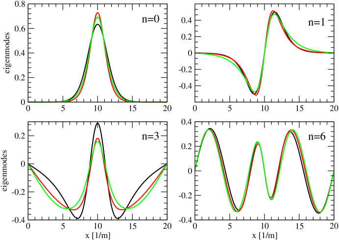
Figure 1: Four of the lower eigenmodes ($n=0,1,2,6$, clockwise) in the 1-loop approximation (red), 1-loop resummed in $G$ (green) and full problem including backreaction on $\varphi$ (black).

At 1-loop order the spectrum of fluctuations about the classical kink is also known exactly. The spectrum consists of two discrete modes with eigenvalues $\omega^{2}_{0}=0$, $\omega^{2}_{1}=\frac{3}{2}m^{2}$ lying below a continuum with $\omega^{2}_{k}=k^{2}+2m^{2}$. The corresponding (unnormalized) eigenvectors are

$$g_{0}(x)=\cosh^{-2}z;\qquad g_{1}(x)=\sinh z/\cosh^{2}z,$$ (20)

$$g_{n}(x)=e^{ikx}\left[3\tanh^{2}z-3\sqrt{2}i\tanh z-1-2\frac{k^{2}}{m^{2}}\right].\qquad$$ (21)

with $z=mx/\sqrt{2}$. We verified that to this order our numerical solutions coincide with these results. Fig. 1 shows the eigenvectors obtained numerically for low lying modes. Corresponding eigenvalues and kink rest energies computed at different levels of approximation are summarized in Table  1. The 1-loop results for the mass shift $\delta m$ computed via two different methods (19) and (17) agree well with each other ($-0.4712$ vs. $-0.4742$) and also with the known analytical result at the 1-loop order, $\delta m=-0.4711$, see Refs. Dashen ; Rajaraman ; BT ; Weidig . Beyond this point no exact analytical results are known.

As a first step beyond 1-loop, we may consider solving the self-consistent problem Eq. (12) without backreaction on $\varphi$. This case has been studied by Boyanovsky et al. Boyanovsky who devised a variational approach, based on the knowledge of the 1-loop perturbative spectrum. They assume that a solution for the fluctuation modes can be constructed by treating the inverse width of the kink potential $A$ and the asymptotic fluctuation mass $M$ as variational parameters and using the eigenvalue equation to determine a relationship between them. If we impose the constraints appropriate to our choices, $A=m/\sqrt{2}$ and $M=\sqrt{2}m$, we can use the solutions of Ref. Boyanovsky to predict the form of the renormalized $G(x)$ to be

$$G(x)=\frac{F(\eta)}{\cosh^{2}(xA)},\ {\rm with}\quad F(\eta)=\frac{\eta}{2\pi}\tan^{-1}(\eta),$$ (22)

where $\eta=A/\sqrt{M^{2}-A^{2}}$ and the lowest eigenvalue to be $\omega^{2}_{0}=M^{2}-A^{2}$. With our choice of parameters this would give $\eta=0.408$, $F(\eta)=0.025$ and $\omega^{2}_{0}=3/2m^{2}$. Instead our numerical solution gives an amplitude for $G$ of 0.226, and $\omega^{2}_{0}=0.50m^{2}$, as we have discussed above. The reason for the discrepancy is that the self-consistent mode profiles, although reminiscent of their 1-loop forms, display a different width both from the classical kink profile and from each other. This allows them to considerably lower their associated eigenvalues and leads to a much larger $G$ than in Ref. Boyanovsky . In other words, the self-consistency in $G$ creates a repulsive effect (a decrease in the depth of the attractive potential provided by the classical kink) in (12) and therefore leads to larger bound-state eigenvalues, which are the principal source of the energy shifts. As a consequence the quantum kink energy is now higher than at 1-loop, but still smaller than its classical value. Results for the first few modes are summarized in Table 1.

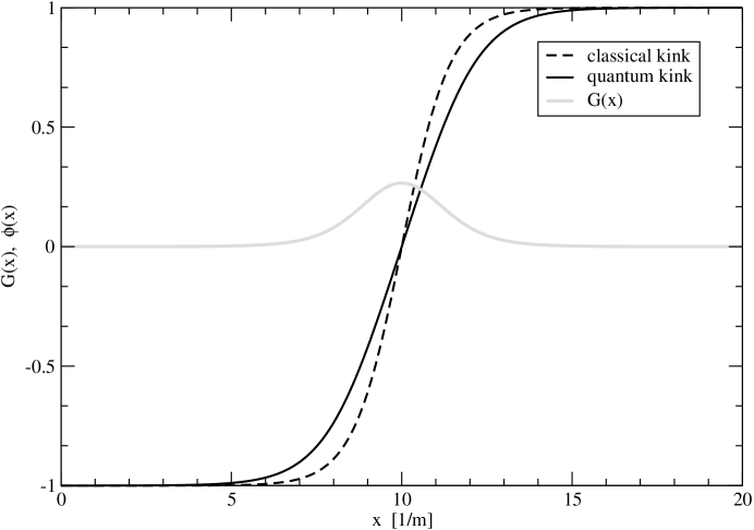
Figure 2: The profiles of the quantum kink, its classical counterpart and $G(x)$ for $\lambda=\hbar=1$

The fully self consistent solution, including backreaction on the mean-field, is shown in Fig. 2. The most important qualitative change to the fluctuation spectrum is that the lower lying modes become more tightly bound relative to the 1-loop resummed case, see Table 1, and that a third (shallow) bound state appears. The kink mean-field profile is now broader than its classical counterpart. Although the self-consistent mean-field solution is not perfectly fit by a $\tanh(xA)$, we can quantify this effect by producing a best value $A=m/2.07$ [c.f. $A=m/\sqrt{2}$ for the classical kink]. The broadening of the mean-field raises the classical energy but this energy cost is more than compensated for by the lowering of the fluctuation spectrum. Allowing the mean-field profile to relax to a more favorable configuration leads to the lowering of the self-consistent kink energy. Nevertheless the effects of the fluctuation self-interactions still result in a total energy higher than at 1-loop. The response of the mean-field and fluctuations taken together, self-consistently, can be thought of as a screening effect of the defect by the fluctuations. The mass of the self-consistent kink in this approximation is in excellent agreement with the lattice results of Ref. Ardekani .

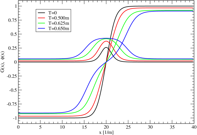
Figure 3: Quantum kink profiles at different temperatures. The kink mean field profile broadens with temperature and eventually disappears at $T\simeq 0.65m$.

Finally we investigate the effects of turning on temperature, see Fig. 3. Numerically this is best achieved by slowly increasing $T$ and successively constructing solutions at higher temperature from previous results at lower $T$. Fig. 3 shows that the kink broadens as the temperature is increased. At $T\simeq 0.65m$ the solution starts probing a new local minimum around $\varphi=0$, which is an inadequacy of the approximation (the Hartree approximation predicts a first-order thermal phase transition for the $\phi^{4}$ model, which is known to have a second order transition). However, as the kink energy now becomes comparable to the temperature, it is plausible that a stable kink no longer exists; our numerical methods invariably converge to the trivial $\varphi=0$ solution. In a model with a true second order phase transition one may expect self-consistent defects to persist and broaden all the way up to $T=T_{c}$, where they may melt away (their core size diverges) and cease to be localized objects.

In summary we constructed a fully self-consistent solution for a topological defect, including the back-reaction of quantum fluctuations at the level of the Hartree approximation. We have shown that at zero temperature the self-consistent dressed kink is lighter than its classical counterpart–the kink is still attractive and leads to a lower lying spectrum of fluctuations relative to the vacuum–but heavier than the well known 1-loop result, due to the repulsion among self-consistent fluctuations. At finite temperature the effects of fluctuations are enhanced by a thermal population of low lying modes and the kink becomes ever broader as the temperature is increased until it vanishes.

We thank D. Boyanovsky, F. Cooper, R. Jackiw, B. Jaffe, K. Rajagopal, N. Svaiter and H. Weigel for discussions and comments. LB benefited additionally from discussions with F. Alexander, F. Cooper, S. Habib and E. Mottola, where the idea of the present paper originated. This work was supported in part by the D.O.E. under research agreement $\#$DF-FC02 94ER40818 and the DOE/BES Program in the Applied Mathematical Sciences, Contract KC-07-01-01.

References

- (1) R. Rajaraman, Solitons and Instantons (North-Holland, Amsterdam, 1982).
- (2) A. Vilenkin and E.P.S. Shellard, Cosmic Strings and other topological defects (Cambridge Univ. Press, Cambridge, 1994).
- (3) L. Kadanoff, Statistical Physics: Statics, Dynamics and Renormalization (World Scientific, Singapore, 2000).
- (4) A. M. Polyakov, Gauge fields and strings (Harwood Academic, New York, 1987).
- (5) T. W. Kibble, J. Phys. A 9, 1387 (1976).
- (6) S. Habib and G. Lythe, Phys. Rev. Lett. 84, 1070 (2000)
- (7) Y. Bergner and L. M. Bettencourt, arXiv:hep-ph/0206053.
- (8) E. Farhi, N. Graham, R. L. Jaffe and H. Weigel, Phys. Lett. B 475, 335 (2000) Nucl. Phys. B 585, 443 (2000)
- (9) H. J. de Vega, Nucl. Phys. B 115, 411 (1976); J. Verwaest, Nucl. Phys. B 123 (1977) 100.
- (10) D. Boyanovsky, F. Cooper, H. J. de Vega and P. Sodano, Phys. Rev. D 58, 025007 (1998)
- (11) For an overview of the literature on the self-consistent time evolution of quantum fields see E. Calzetta and B. L. Hu, Phys. Rev. D 35, 495 (1987); F. Cooper et al., Phys. Rev. D 50, 2848 (1994); D. Boyanovsky et al., Phys. Rev. D 51, 4419 (1995); J. Berges, Nucl. Phys. A 699, 847 (2002) F. L. Braghin, Phys. Rev. D 64, 125001 (2001); L. M. A. Bettencourt, K. Pao and J. G. Sanderson, Phys. Rev. D 65, 025015 (2002).
- (12) G. D. Moore, Phys. Rev. D 53, 5906 (1996)
- (13) W. Schroers, I. Bornig, C. Schulzky and K. Goeke, arXiv:hep-ph/9801438.
- (14) A. Ardekani and A. G. Williams, Austral. J. Phys. 52, 929 (1999). We thank M. Sallé for pointing out this reference to us. A partial computation in the same spirit as our analysis is worked out independently in his Ph.D. thesis.
- (15) Y. Bergner and L.M.A. Bettencourt, The self-consistent bounce, in preparation.
- (16) The relativistic formalism was developed in J. M. Cornwall, R. Jackiw and E. Tomboulis, Phys. Rev. D 10, 2428 (1974). For nonrelativistic precursors, see also J. M. Luttinger, J. C. Ward, Phys. Rev. 118 (1960) 1417; G. Baym, Phys. Rev. 127 (1962) 1391.
- (17) R. F. Dashen, B. Hasslacher and A. Neveu, Phys. Rev. D 10, 4130 (1974); R. F. Dashen, B. Hasslacher and A. Neveu, Phys. Rev. D 11, 3424 (1975).
- (18) K. Cahill, A. Comtet and R. J. Glauber, Phys. Lett. B 64, 283 (1976).
- (19) C. Barnes and N. Turok, arXiv:hep-th/9711071.
- (20) T. Weidig, arXiv:hep-th/9912005.
- (21) A. Rebhan and P. van Nieuwenhuizen, Nucl. Phys. B 508, 449 (1997)
- (22) We used the standard relaxation routine solvde from W. H. Press et al., Numerical recipes in Fortran 77 and Fortran 90, (Cambridge Univ. Press, Cambridge, U.K., 1996).
- (23) Specifically we used the suboutine SSYEV appropriate for real-symmetric operators, see http://www.netlib.org/lapack/ for full reference.