hep-th/0305188

Superconformal D-branes
and moduli spaces

Cecilia Albertsson

Doctoral Thesis in

Theoretical Physics

Department of Physics

Stockholm University

2003

Thesis for the degree of doctor of philosophy in theoretical physics
Department of Physics, Stockholm University
Sweden
© Cecilia Albertsson 2003
ISBN 91-7265-630-1 (pp i-ix, 1-64)
Akademitryck AB, Edsbruk

Abstract

The on-going quest for a single theory that describes all the forces of nature has led to the discovery of string theory. This is the only known theory that successfully unifies gravity with the electroweak and strong forces. It postulates that the fundamental building blocks of nature are strings, and that all particles arise as different excitations of strings. This theory is still poorly understood, especially at strong coupling, but progress is being made all the time. One breakthrough came with the discovery of extended objects called D-branes, which have proved crucial in probing the strong-coupling regime. They are instrumental in realising dualities (equivalences) between different limits of string theory.

This thesis is concerned with dualities and D-branes. First, it gives a background and review of the first article, where we substantiated a conjectured duality between two a priori unrelated gauge theories. These gauge theories have different realisations as the worldvolume theories on different D-brane configurations. We showed that there is an identity between the spaces of vacua (moduli spaces) arising in the two theories, which suggests that the corresponding string theory pictures are dual.

Second, we give a background and description of the analysis performed in the remaining three articles, where we derived the most general, local, superconformal boundary conditions of the two-dimensional nonlinear sigma model. This model describes the dynamics of open strings, and the boundary conditions dictate the geometry of D-branes. In the last article we studied these boundary conditions for the special case of WZW models.

Chapter 1 Introduction

“This sort of thing has cropped up before,

and it has always been due to human error.”

— HAL 9000,   in   2001: A Space Odyssey

Although the film’s supercomputer was referring to a faulty communications device, its statement turned out to carry universal truth, much to the dismay of the ill-fated crew of Discovery. And not only was the fault indeed induced by humans, it was of a fundamentally different nature than the crew initially thought.

This is characteristic of research in theoretical physics. The quest for an ultimate theory that will explain all the forces of nature in a single, beautiful principle, is a typically human one. Besides a curiosity about the world around us, we are driven by our desire for aesthetics and simplicity. Sometimes so much so that we are tempted to make oversimplified assumptions about nature, such as the Aristotelian “natural state,” or Copernicus’ circular planetary orbits. We may be unaware of the error, building entire theories on our flawed axioms, and not until disaster strikes do we realise just how fundamental a mistake we have made.

It is easy to make such mistakes because nature often turns out to be much more peculiar than we ever imagined, displaying counterintuitive effects like the particle-wave duality. At first, such weirdness might be misconstrued as complications. But going along with it usually in the end leads to an even simpler picture of the world, bringing us closer to a unified theory of everything. So as a physicist, one learns to accept ridiculous ideas just for the sake of argument.

One such “ridiculous idea” constitutes the foundation of string theory.

1.1 Strings

The idea is that all elementary particles are actually vibrating strings.

This was put forward by phycisists in the seventies, after failing to use string theory to describe the strong interactions (quantum chromodynamics does a better job of that). It was realised that string theory unifies gravity with the three forces described by quantum field theory — electromagnetism, the weak force and the strong force. Because the basic building blocks are one-dimensional objects, strings, instead of zero-dimensional point particles, string theory does not suffer from the divergences of quantum field theory.

The fact that strings are one-dimensional leads to a vast range of possible string states. Strings can be open (two ends) or closed (ends joined), and they can oscillate in a multitude of ways. The different states that arise in this way correspond to different particles. That is, instead of the plethora of fundamental particles in the Standard Model, we have only one type of fundamental object; all matter can be explained as strings in different states.

But string theory is not a simple theory, in any sense of the word. What keeps string theory a field in development is the fact that it is technically very difficult, often impossible, to perform exact calculations. One is frequently forced to approximate, or resort to hand-waving. Furthermore, string theory is actually not a single theory; it is five different theories, all individually consistent, but with different characteristics. Some describe only closed strings, others both open and closed, the strings may be oriented or unoriented, and the theories have different symmetries, etc. At first sight these theories seem to be very far from anything resembling realistic physics. For one thing, they are in general supersymmetric, i.e. they demand the existence of superpartners of all observed particles, none of which have shown up in experiments as yet. Another nuisance is their requirement of no less than ten spacetime dimensions to live in.

Nevertheless, in the course of time there has been an increasing amount of order brought to this mess, in the form of symmetries and dualities. It turns out that the five string theories are related to each other via various dualities, so that they are manifestly equivalent in different limits. One nice thing about this is that computations that are difficult in one picture may become easier in the dual picture. More interestingly, there is mounting evidence that, at the end of the day, all these theories are just different limits of one and the same underlying theory, our holy grail. This is why the understanding of dualities in string theory is of paramount importance.

1.2 D-branes

In the nineties, it was discovered that in addition to strings, string theory contains other types of extended dynamical objects, called Dirichlet branes (D-branes). The name comes from their function as hypersurfaces on which open strings can end — an endpoint stuck to a D-brane obeys Dirichlet conditions. They can be of any dimension as long as it fits inside the ten dimensions of string theory. D-branes play a crucial role in relating the different string theories to each other, primarily via their transformation properties under duality.

One way of dealing with the six surplus spacetime dimensions (since we experience only four), is to compactify them on tiny spaces, like wrapping a piece of paper around a pencil. From a distance the paper then looks one-dimensional, and we are rid of one dimension. Besides reducing the number of dimensions, this technique has the advantage that the “compact” part of the string theory shows up as matter in the noncompact dimensions. We can thus construct the four-dimensional theory of our choice by compactifying on the appropriate manifold.

In this context D-branes are useful for visualising where in the ten-dimensional string theory our four-dimensional world fits. If we choose a D-brane with four spacetime dimensions (a D3-brane), then the part of string theory that lives on its worldvolume would describe the physics of the universe as we know it. Of course we would need to break a lot of symmetries first, especially supersymmetry, but in essence this is the picture.

1.3 Outline

This thesis is divided into two chapters; the first one is concerned with Paper I, and the second with Papers II–IV.

Moduli spaces

The realisation of physics as the worldvolume theory of a D-brane is the topic of Chapter 2. After providing some basics concerning Lie algebras, we discuss the rather multifaceted background of Paper I. The centre of attention is the space of vacua (moduli) in the worldvolume theory of D3-branes, which splits into different branches depending on the particular configuration we are looking at. We explain how these branches of vacua arise, first from a purely field-theoretical point of view, and then from a string theory perspective. The object of Paper I was to show the equivalence between the moduli spaces of two different theories, the E₈ quiver gauge theory, and the E₈ Seiberg-Witten theory, in order to substantiate a conjectured duality between them. We define these two theories and give a brief account of the method used to compare the moduli spaces.

Boundary conditions

The dynamics of open superstrings is described by the supersymmetric non-linear sigma model, which is a field theory in two dimensions. The domain of this model is the two-dimensional worldsheet of the string, i.e. the surface that the string sweeps out as it moves through spacetime. Since the string has two ends, this domain has two boundaries, which by definition are attached to D-branes. So studying boundary conditions of the sigma model is equivalent to studying the geometrical properties of D-branes.

In particular, these conditions should be consistent with the way D-branes transform under duality. For instance, T-duality changes the dimension of the D-brane, and the duality transformation acting on the boundary conditions should yield the same result. This was our prime motivation in deriving the most general boundary conditions possible, in Papers II–III. More precisely, we derived superconformal boundary conditions, i.e. conditions for the boundary to respect the super- and conformal symmetries that are preserved in the bulk of the worldsheet. Chapter 3 provides some background to that derivation and explains how it was done. In Paper IV we applied our analysis to the WZW model, a special case of the nonlinear sigma model; the last section is devoted to that.

1.4 About the thesis

This thesis touches on many different topics, from F-theory to almost product structures, all of them incredibly rich fields. We will not go into great depth in any of these subjects, only give a brief review of those aspects that are directly relevant to the accompanying papers. I have tried to keep the discussion on a basic level, for the most part assuming that the reader is not an expert. However, it has proven unavoidable to sometimes state facts without justification, where an explanation would be much too involved. I have also tried to make each chapter selfcontained, but inevitably, Chapter 3 does make use of some concepts introduced in Chapter 2.

Moreover, as frequently becomes apparent in string theory, computational techniques, and even notation, are not of secondary importance. This is definitely true in the work presented here, where reaching the goal depended crucially on the method of getting there. Despite this, we will not linger on technical details, only mention briefly the approach taken in each case.

The interesting part is after all the conclusions. They clarify but a small fraction of the huge scientific effort which is string theory, but I still believe that this theory is the path to follow in our search for the ultimate principle.

Indeed, there is every indication that string theory is not merely a misconception, due to human error.

Chapter 2 Moduli spaces

2.1 Introduction

In this chapter we will be dealing with four-dimensional supersymmetric gauge theories and their moduli spaces, realised as worldvolume theories on D3-branes. The exact worldvolume action (i.e. including massive fields) on a D-brane is not known, although considerable effort is being invested in finding it [1, 2]. So reliable analysis is possible strictly in the low-energy effective theories, where only massless fields are considered. Such theories are described by super-Yang-Mills theories, which will be our main concern here.

In particular, we are interested in the spaces of vacua in the Yang-Mills theories. These are obtained by applying the Higgs mechanism to the scalar potential; this mechanism renders gauge bosons massive via spontaneous symmetry breaking, and is a candidate for explaining the origin of mass. In ${\cal N}$=2 super-Yang-Mills theory it gives rise to two moduli space branches, the Coulomb branch and the Higgs branch. In string theory, this moduli space corresponds to the space transverse to D-branes sitting in ten dimensions.

To construct four-dimensional theories from string theory, one usually compactifies the “superfluous” dimensions on very small spaces so that they become invisible in everyday, low-energy physics. These compact spaces are subject to a set of restrictions in order that the resulting theory be consistent; such spaces are known as Calabi-Yau manifolds [3]. A complex-one-dimensional Calabi-Yau manifold is topologically always a torus, while in two complex dimensions all Calabi-Yau manifolds are topologically equivalent to the K3 surface [4]. The latter space has orbifold singularities and is the one relevant to us here. The great thing about string theory in this context is that it remains well-behaved even when compactified on singular spaces such as these orbifolds.

2.1.1 Mirror symmetry

It is believed that most, if not all, Calabi-Yau manifolds have an associated mirror manifold, i.e. a manifold whose complex structure moduli are exchanged with the Kähler structure moduli as compared to the original Calabi-Yau [4]. This is a very important result since it has an implication that string theories compactified on two mirror manifolds are equivalent (dual) to each other. As a consequence, if the moduli spaces of two conformal field theories make up a mirror pair, then the corresponding theories are dual to each other [3, 5].

Intriligator and Seiberg [6] showed how a duality between two different gauge theories in three dimensions corresponds to a mirror symmetry between their respective moduli spaces. The two kinds of theories are, on the one hand, three-dimensional ADE quiver theories (as constructed by Kronheimer [7]), and on the other hand $SU(2)$ gauge theory with ADE global symmetry (Seiberg-Witten theory). This mirror symmetry exchanges the Coulomb branch of one theory with the Higgs branch of the other, and vice versa. The two branches are in fact geometrically identical, but the mirror exchange is interesting from a physics point of view. In particular, the mass parameters (which are associated with complex structure) of one theory are interchanged with the Fayet-Iliopoulos parameters (associated with Kähler structure) of the other theory.

Since the four-dimensional versions of these theories are related to the three-dimensional ones via compactification, one might suspect that there is a similar mirror symmetry acting in four dimensions. In fact, a Higgs-Coulomb identity analogous to that of the three-dimensional case was confirmed in [8], for the $A_{1}$, $A_{2}$, $D_{4}$ and $E_{6}$ four-dimensional theories. The remaining two of the strongly coupled superconformal ${\cal N}$=2 theories, $E_{7}$ and $E_{8}$, were shown to also satisfy such Higgs-Coulomb identities, in [9] and Paper I, respectively. Just like in three dimensions, the four-dimensional mirror symmetry would provide a map between mass parameters of one theory and Fayet-Iliopoulos parameters of the other.

One very useful consequence of such a mirror symmetry is that, since the Coulomb branch receives quantum corrections but the Higgs branch does not (due to ${\cal N}$=2 supersymmetry), quantum effects in one theory arise classically in the dual theory, and vice versa. This facilitates the analysis of nonperturbative phenomena enormously. Although the $E_{8}$ theory does have some interest in itself, for instance in explaining the $E_{8}$ gauge symmetry of the heterotic string, the main motivation for establishing the moduli space equivalence for $E_{8}$ was to complete the analysis for the whole series of strongly coupled superconformal ${\cal N}$=2 theories. Knowing that there is a true duality between the quiver theory and the Seiberg-Witten theory, one could use this to analyse the quantum behaviour of physically more interesting theories such as $D_{4}$.

2.1.2 Outline

Clearly, some knowledge of simple Lie algebras is required, so we start by listing some fundamental facts about these in Section 2.2. We then move on to discuss ${\cal N}$=2 supersymmetric Yang-Mills theories in Section 2.3, showing how the moduli space of vacua arises as a result of the Higgs mechanism. Next, we define the two different gauge theories involved in the duality discussed above, namely Seiberg-Witten theory (Section 2.4) and quiver theory (Section 2.5). The latter section ends with a brief account of the computation done in Paper I.

Before proceeding, however, let us clarify a fundamental point, namely the difference between “perturbative” and “low-energy effective.” A theory can be treated perturbatively when the coupling constant is so small that an expansion in powers of the coupling constant is dominated by the first few terms. On the other hand, a theory is a low-energy effective theory when any massive states are so heavy compared to some fixed energy scale (e.g. the cutoff scale in renormalisation) that they completely decouple from the theory. Thus, for instance, the Seiberg-Witten theory is a strongly coupled gauge theory where we have discarded all massive states and retain only the massless ones.

With that, we are ready to embrace some representation theory.

2.2 Lie algebras

Lie algebra theory is an essential instrument in a physicist’s mathematical toolbox. This is due to the close connection to vector fields on manifolds, the most important example of which are those on spacetime. As the name suggests, Lie algebras are the algebras of Lie groups, which by definition are groups endowed with the properties of a smooth manifold. Examples of such groups are $GL(n,{\mathbb{R}})$, $SL(n,{\mathbb{R}})$ and $SO(n,{\mathbb{R}})$. The $C^{\infty}$ vector fields on such a manifold form a Lie algebra. We will be concerned only with simple Lie algebras, i.e. Lie algebras of finite dimension greater than one and which contain no nontrivial ideals. The complete list of such algebras is not extensive, but the only ones relevant to us are: $A_{n}$, $D_{n}$, $E_{6}$, $E_{7}$ and $E_{8}$. The first two correspond to the groups $SL(n+1,{{\mathbb{C}}\,})$ and $SO(2n,{{\mathbb{C}}\,})$ respectively, whereas the $E_{n}$ algebras correspond to three exceptional groups, defined e.g. in [10]. These groups are usually referred to collectively as ADE symmetries and, somewhat confusingly, we sometimes use the algebra notation to denote the corresponding groups.

In this section we give the standard definitions of some Lie algebra objects that will be useful in the subsequent discussion.

2.2.1 Definitions

The Lie algebra $\mathfrak{g}$ is related to its Lie group $G$ by the exponential map $\exp:\mathfrak{g}\rightarrow G$; i.e. $\exp(X)\in G$ for any element $X\in\mathfrak{g}$ . This defines it as a representation of its Lie group. That is, it is a homomorphism from $G$ to the group of automorphisms of the tangent space of $G$ at the identity, $\rho:G\rightarrow\textstyle{\mathrm{Aut}}(T_{e}G)$ [10]. It comes equipped with a Lie bracket, defined as

$$[T^{a},T^{b}]=f^{ab}_{\,\,\,\,\,\,\,c}T^{c},$$ (2.1)

where $T^{a}$ are the Lie algebra generators and $f^{ab}_{\,\,\,\,\,\,\,c}$ are structure constants. This bracket is a kind of product structure, a bilinear form mapping any two elements in $\mathfrak{g}$ to a third. As such it is used to construct the adjoint representation of the group $G$, defined as

$$\textstyle{\mathrm{ad}}_{X}Y\equiv[X,Y],\quad\quad X,Y\in\mathfrak{g}.$$

The Lie bracket in principle defines the whole, rather rich, structure of the algebra. In particular, it defines the roots, which are eigenvalues of $\textstyle{\mathrm{ad}}_{h}$, with $h$ any element in the Cartan subalgebra $\mathfrak{h}\subset\mathfrak{g}$. By a Cartan subalgebra we mean a maximal abelian subalgebra such that the maps $\textstyle{\mathrm{ad}}_{h}:\mathfrak{g}\rightarrow\mathfrak{g}$ can be simultaneously diagonalised for all $h\in\mathfrak{h}$. There are two types of roots, positive and negative, which we denote by $w_{+}$ and $w_{-}$, respectively; they are simply related by $w_{-}=-w_{+}$. Any root can be expressed as a linear combination of a number of simple roots with integer coefficients. Positive roots are written with positive coefficients and negative roots with negative coefficients in their simple-root-decomposition. The number of simple roots is equal to the rank of the Lie algebra; for instance, $E_{8}$ has eight simple roots.

2.2.2 Finding the roots

Roots satisfy a number of conditions which may be used to derive the full set of positive roots [10]. As this was exploited in Paper I for the $E_{8}$ roots, we will demonstrate the procedure for that particular case here, but first we need to define another crucial ingredient in the Lie algebra setup, the Cartan matrix. This is essentially a matrix of inner products between simple roots. More precisely, the entries of the Cartan matrix $C$ associated with the Lie algebra $\mathfrak{g}$ are defined as

$$C_{ij}\equiv 2(\alpha_{i},\alpha_{j})/(\alpha_{j},\alpha_{j}),$$

where $\alpha_{i}$ are the simple roots, $i=1,...,\textstyle{\mathrm{rank}}(\mathfrak{g})$, and $(\,\cdot\,,\,\cdot\,)$ is the inner product on $\mathfrak{g}$. The diagonal elements are always equal to 2, while the off-diagonal elements are either zero or negative. For $\mathfrak{g}=E_{8}$ we have

$$C = \left(\begin{array}[]{cccccccc}2&-1&0&0&0&0&0&0\\ -1&2&-1&0&0&0&0&0\\ 0&-1&2&-1&0&0&0&0\\ 0&0&-1&2&-1&0&0&0\\ 0&0&0&-1&2&-1&0&-1\\ 0&0&0&0&-1&2&-1&0\\ 0&0&0&0&0&-1&2&0\\ 0&0&0&0&-1&0&0&2\\ \end{array}\right).$$

To find the full set of (positive) roots, we first choose a root $w_{0}=\sum_{i}m_{i}\alpha_{i}$ such that

$$(w_{0},\alpha_{1})=1,\quad\quad(w_{0},\alpha_{i})=0,\,\,i\neq 1.$$

Then the root properties imply that $w_{0}-\alpha_{1}$ is another positive root. Next, we take the inner product of this new root with each of the simple roots to see which one gives a positive result,

$$(w_{0}-\alpha_{1},\alpha_{1}) = 1-2=-1,$$

$$(w_{0}-\alpha_{1},\alpha_{2}) = 0+1=1,$$

$$(w_{0}-\alpha_{1},\alpha_{i}) = 0+0=0,\quad\quad i>2.$$

Thus the next positive root is obtained as $w_{0}-\alpha_{1}-\alpha_{2}$, and so on. One can show that the resulting set of roots from this algorithm is the full set [10]; for $E_{8}$ we find 120 positive roots.

The reader may notice that we are dealing with weights rather than roots in Paper I. The reason the above procedure is still applicable is as follows. Corresponding to each representation ${\cal R}$ of a Lie algebra $\mathfrak{g}$, there is a set of weights, the eigenvalues of $\mathfrak{h}$ in this representation. If ${\cal R}$ is the adjoint representation $\textstyle{\mathrm{ad}}_{h}$, then the weights are precisely the roots of the Lie algebra. And since the fundamental representation of $E_{8}$ is the same as the adjoint one, finding the weights of the fundamental representation is in fact equivalent to finding the roots of $E_{8}$.

2.2.3 Dynkin diagrams

All the structure and properties of any simple Lie algebra can be encoded in a simple graph called a Dynkin diagram. Such a diagram consists of a number of nodes linked by edges. Each node corresponds to a simple root, and the number of edges between each pair of nodes reflects the value of the inner product between those two simple roots. There is a direct relation between the entries of the Cartan matrix and the number of edges $N_{ij}$ between the simple roots $\alpha_{i}$ and $\alpha_{j}$, $N_{ij}=C_{ij}C_{ji}$.

This kind of diagram is very powerful as an algebra representation because, given a Dynkin diagram, you can recover the whole structure of the corresponding Lie algebra. The $E_{8}$ Dynkin diagram is shown in Fig. 2.1.

Figure 2.1: The $E_{8}$ Dynkin diagram. Each node corresponds to a simple root $\alpha_{i}$, and the number of edges between each pair of nodes is given by the Cartan matrix elements as $N_{ij}=C_{ij}C_{ji}$ ; compare to the $E_{8}$ Cartan matrix given in Section 2.2.2.

2.3 $\mathbf{{\cal N}}$=2 super-Yang-Mills theory

Yang-Mills theory is essentially a synonym for nonabelian gauge theory. That is, it is a field theory that is invariant under local (or gauge) transformations, i.e. spacetime dependent transformations, which form a nonabelian group. In four dimensions such a theory can be used to describe three of the four forces of nature at low energy. When the theory has gauge symmetry group $SU(3)$, it describes the strong interactions and is known as quantum chromodynamics (QCD). For $SU(2)\times U(1)$ it unifies electromagnetic and weak interactions in the electroweak theory. Together, QCD and the electroweak theory constitute the Standard Model, which to date reproduces all known experimental results of particle physics.

A gauge theory may possess other symmetries in addition to the gauge symmetry. For example there may be a global symmetry group; that is, the theory is invariant under some group of spacetime independent transformations. The intuitive physical picture of such a global symmetry is as a symmetry acting on added matter, for instance a number of quarks in QCD.

Another symmetry example is supersymmetry, i.e. a symmetry between bosons and fermions such that every boson is matched by a fermion (a “superpartner”) with equal mass and charge. It may seem unmotivated to introduce such a symmetry, since in experiments we have seen neither spin-0 particles with the mass of an electron, nor massless spin-$\frac{1}{2}$ particles (“photinos”). But the idea is that the low-energy world we live in has spontaneously broken supersymmetry, while at sufficiently high energy we would see the supersymmetry manifest. One promising clue that this might be the case comes from the standard model coupling constants. The theoretical prediction is that, without supersymmetry, they all are almost, but not quite, equal, at around $10^{14}$ GeV, whereas inclusion of supersymmetry makes them exactly identical, at an energy of around $10^{16}$ GeV.

If a nonabelian gauge theory is supersymmetric, it is called super-Yang-Mills (SYM) theory. Such a theory is also invariant under so-called R-symmetry, which is essentially the symmetry group transforming the different supersymmetry generators into each other.

We now define the precise type of SYM theories that interest us, before embarking on an analysis of their vacuum states.

2.3.1 Defining our SYM theory

There are several parameters we need to specify in order to define which particular type of SYM theory that we are interested in. First, SYM theory can be defined in any dimension up to ten (see [5], Appendix B), but the case relevant to us is the four-dimensional one (as the low-energy effective action on a D3-brane).

We also need to specify the number of supersymmetries, ${\cal N}$. Although the worldvolume theory in Paper I a priori has ${\cal N}$=$4$ (see [5], Chapter 13), this supersymmetry is partially broken by putting the branes on an orbifold singularity, and we end up with ${\cal N}$=2. So we focus here on ${\cal N}$=2 SYM theory.

The next thing to specify is the field content.

Field content

A SYM theory contains a number of massless multiplets; the larger, massive multiplets can always be decomposed into these. The relevant multiplet in “pure” ${\cal N}$=$2$ SYM theory (i.e. there are only gauge field interactions in the theory, and no matter added by hand) is a vector multiplet containing gauge fields $A^{a}_{\mu}$ ($a$ labels the gauge group generators), two spinors $\lambda^{a}_{\alpha}$ and $\chi^{a}_{\alpha}$, a complex scalar $\varphi^{a}$ and a real auxiliary field $D^{a}$ (see [5], Appendix B.2).

All these fields transform in the adjoint representation of the gauge group. This means that, under a transformation by an element $g$ of the gauge group, a field $\phi$ transforms as

$$\phi\rightarrow g\phi g^{-1}.$$

On the other hand, it is said to transform in the fundamental representation if it transforms as

$$\phi\rightarrow g\phi,\quad\quad\phi^{\dagger}\rightarrow\phi^{\dagger}g^{-1},$$

where $\phi^{\dagger}$ is the Hermitian conjugate of $\phi$. Finally, $\phi$ is said to transform in the antifundamental representation of $G$ if it transforms as

$$\phi\rightarrow\phi g^{-1},\quad\quad\phi^{\dagger}\rightarrow g\phi^{\dagger}.$$

Sometimes the representations are denoted by fat numbers, so that a field transforming in the fundamental representation of, say, $U(3)$, is said to transform as $\mathbf{3}$ (3 is the dimension of this representation). The antifundamental analogue is $\mathbf{\bar{3}}$. Note that a field transforming in both $\mathbf{3}$ and $\mathbf{\bar{3}}$ of $U(3)$ by definition transforms in the adjoint. Moreover, if a field transforms under a product of groups, say $U(2)\times U(3)$, as $(\mathbf{2},\mathbf{\bar{3}})$, then we call it a bifundamental field. This notation will be relevant when we discuss quiver gauge theories in Section 2.5.

We now add some fundamental matter to our pure ${\cal N}$=2 SYM theory. More precisely, we introduce two hypermultiplets, each of which consists of a complex scalar field $\phi^{i}$ ($i=1,2$ labels the two hypermultiplets), a spinor $\psi^{i}$ and a complex auxiliary field $F^{i}$, and they all transform in the fundamental representation of the gauge group.

2.3.2 Spontaneous symmetry breaking

Due to the shape of the potential in ${\cal N}$=2 SYM theory, the gauge symmetry may be spontaneously broken. This happens because, instead of a unique vacuum with zero energy, there is a whole family of vacua. Rather than being individually invariant under gauge symmetry transformations, these vacua are transformed into each other. The physical system will spontaneously choose one of the vacua, thus breaking the gauge symmetry. This process goes by the name Higgs mechanism, a physical example of which is superconductivity (see e.g. [11], Chapter 8). The gauge-broken theory describes the dynamics of the chosen vacuum field, which parameterises the moduli space, i.e. the space of vacua, of the theory.

To illustrate the principle of the Higgs mechanism, we now consider the bosonic Yang-Mills theory with $SU(2)$ gauge symmetry.

SU(2) bosonic Yang-Mills

We first write down the Lagrangian and then define the constituent fields. The Yang-Mills Lagrangian, with one matter (complex scalar) field $\phi$ transforming in the fundamental representation of the gauge group, is (see [11], Section 8.3)

$${\cal L}_{YM}=-(D^{\mu}\phi)^{\dagger}(D_{\mu}\phi)-V(\phi^{\dagger}\phi)-\frac{1}{4}\sum^{3}_{a=1}F^{a}_{\mu\nu}F^{a\mu\nu}.$$ (2.3)

Since $\phi$ transforms in the fundamental representation of $SU(2)$, we can write it as a doublet,

$$\phi(x^{\mu})=\left(\begin{array}[]{c}\phi^{1}(x^{\mu})\\ \phi^{2}(x^{\mu})\end{array}\right),$$

where $\phi^{1,2}$ are complex functions of the spacetime coordinates $x^{\mu}$.

The field strength $F^{a}_{\mu\nu}$, where $a$ labels the $SU(2)$ generators $T^{a}$ and $\mu,\nu$ are spacetime indices, is defined as

$$F^{a}_{\mu\nu}\equiv\partial_{\mu}A^{a}_{\nu}-\partial_{\nu}A^{a}_{\mu}-igf^{a}_{\,\,\,\,bc}A^{b}_{\mu}A^{c}_{\nu},$$

with $f^{a}_{\,\,\,\,bc}$ being the structure constants of the $SU(2)$ Lie algebra, cf. Eq. (2.1), and $g$ is a coupling constant.

We take the potential $V$ to be

$$V(\phi^{\dagger}\phi)\equiv\frac{1}{2}\lambda^{2}(\phi^{\dagger}\phi-\eta^{2})^{2},$$ (2.4)

where the real number $\eta$ is the vacuum expectation value of $\phi$. In the bosonic theory there is nothing that forces us to choose this particular potential, but in the presence of supersymmetry there will be restrictions on $V$, and we choose (2.4) to make the analogy as close as possible.

Finally, the covariant derivative of $\phi$ is defined as

$$D_{\mu}\phi\equiv(\partial_{\mu}-igT^{a}A^{a}_{\mu})\phi$$

(summation over $a$), where the generators $T^{a}$ are taken to be in the fundamental representation of $SU(2)$; in terms of the Pauli matrices, $T^{a}\equiv\sigma^{a}/2$.

The Higgs mechanism

We are interested in the classical vacua of this theory. These are defined by the vanishing of the potential (2.4), so any vacuum $\phi_{0}$ must satisfy $\phi^{\dagger}_{0}\phi_{0}=\eta^{2}$. As mentioned above, the $\phi_{0}$’s are not themselves gauge invariant, but $V$ is, and there is a continuous family of vacua $\{\phi_{0}\}$ related by $SU(2)$ transformations. These vacua parameterise what is called a “flat” direction.

To see where this terminology comes from, consider the $U(1)$ case, where the vacua (which are now complex numbers) are related to each other by a $U(1)$ transformation, $\phi_{0}^{\prime}=e^{i\alpha}\phi_{0}$. As a function of $|\phi|$, the potential $V(|\phi|^{2})$ then has the shape of a mexican hat, with a minimum at $|\phi|^{2}=\eta^{2}$, where it vanishes, see Fig. 2.2. Moving in a radial direction, either in towards the origin or away from the origin, requires energy, like climbing up a hill. But moving along the minimum at a fixed distance from the origin requires no energy since we are moving along the bottom of the “moat” — this is the flat direction, parameterised by the continuous spectrum of vacua.

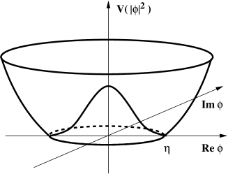
Figure 2.2: The vacuum potential $V(|\phi|^{2})$ of the Lagrangian (2.3), as given by Eq. (2.4). It has a continuous space of vacua at $|\phi|^{2}=\eta^{2}$, for which $V(|\phi|^{2})=0$.

Returning to the $SU(2)$ case, we may now use the gauge freedom to rotate $\phi_{0}$ to a basis where three of its four real components vanish. In other words, we are fixing the gauge by choosing a particular vacuum. The action is no longer invariant under $SU(2)$, so we have broken the gauge symmetry; we have spontaneous symmetry breaking. However, note that the gauge symmetry is not completely broken. The Lagrangian (2.3) is still invariant under $U(1)$ transformations, so the gauge group has been broken from $SU(2)$ down to a $U(1)$ subgroup.

We are thus left with one real component in $\phi_{0}$, which we write as a sum of a constant part $\eta$ and a nonconstant part $\gamma(x^{\mu})$,

$$\phi_{0}=\left(\begin{array}[]{c}0\\ \eta+\gamma(x^{\mu})\end{array}\right).$$ (2.5)

If one inserts (2.5) into the Lagrangian (2.3) and expands the latter, one finds that it contains mass terms for the gauge bosons [12]. That is, there are quadratic terms of the form $m^{2}_{A}A^{a}_{\mu}A^{a\mu}$, where the mass $m_{A}$ is proportional to the parameter $\eta$.

In conclusion, spontaneous breaking of the gauge symmetry renders the gauge bosons massive; in the $SU(2)\times U(1)$ case they combine into the W- and Z-bosons (see [11], Section 8.5). The field $\phi_{0}$ in this context is called a Higgs field, and its vacuum expectation value $\eta$ is the Higgs mass.

2.3.3 The $\mathbf{{\cal N}}$=2 potential

The Higgs mechanism generalises straightforwardly to the supersymmetric theory. The difference is that supersymmetry imposes constraints on the form of the action. For instance, the potential cannot be arbitrary, and in addition the number of scalar fields is restricted.

The action for ${\cal N}$=2 SYM theory is much more complicated than the bosonic one, as it involves all the fields in the vector multiplet ($\varphi^{a}$, $\chi^{a}_{\alpha}$, $\lambda^{a}_{\beta}$, $A^{a}_{\mu}$, $D^{a}$) plus any hypermultiplets $(\phi^{i},\psi^{i},F^{i})$ added by hand, as well as their interactions. In superspace formalism (see Section 3.3 for details) this action looks simpler, but we omit it here since we do not need to work with it explicitly. For a pedagogical account of the ${\cal N}$=2 $SU(2)$ SYM action, see e.g. [13]. Here it suffices to say that to find the potential for the scalar matter fields (which we need for deriving the moduli space), one expands the action in components and extracts all terms containing the auxiliary fields $D^{a}$ and $F^{i}$. This yields a sum of D-terms and F-terms, and then we integrate out $D^{a}$ and $F^{i}$ by use of their equations of motion. The result is a potential involving a sum of commutators between all scalar fields $\varphi^{a}$ and $\phi^{i}$.

Fayet-Iliopoulos terms

However, this is not the whole story. In a supersymmetric gauge theory, the precise form of the potential depends on the number of $U(1)$ factors present in the gauge group. This is because supersymmetry allows an extra term in the action when the gauge group contains a $U(1)$ factor (see [5], Appendix B). This extra term is of the form $\xi^{k}D^{k}$, with $D^{k}$ being the $k$:th $U(1)$-component of $D^{a}$, and $\xi^{k}$ is a real parameter, called the Fayet-Iliopoulos term (FI-term). Thus the FI-parameter corresponding to the generator $T^{a}$ is $\xi^{a}$ with $a$ running over all the gauge group generators, but with $\xi^{a}\neq 0$ only for $a=k$, where $k$ labels the $U(1)$ generators.

In ${\cal N}$=1 SYM there is only one, real FI-term for each $U(1)$ factor. ${\cal N}$=2 supersymmetry, on the other hand, allows three different FI-parameters for each $U(1)$; this is due to the $SU(2)$ R-symmetry that relates the two supersymmetries. The three FI-terms transform as a triplet under the $SU(2)$ R-symmetry [14], and we denote them as a three-vector $\vec{\xi}^{a}$.

The potential

Let us finally have a look at the potential for the scalar fields in our SYM theory:

$$V=\mathrm{Tr}([\varphi,\varphi^{\dagger}]^{2})+\sum_{i=1,2}\phi^{\bar{i}}[\varphi,\varphi^{\dagger}]\phi^{i}+\sum^{\dim G}_{a=1}\left(\mathrm{Tr}\left[T^{a}\cdot\vec{\mu}\right]-\vec{\xi}^{a}\right)^{2},$$ (2.6)

where a barred index implies Hermitian conjugate, $\phi^{\bar{i}}\equiv\phi^{i\,\,\dagger}$. The three-vector $\vec{\mu}$ is defined as

$$\vec{\mu}\equiv\mathrm{Tr}\left(\phi^{\dagger}\vec{\sigma}\phi\right),$$ (2.7)

where $\phi$ is the quaternion of the $\phi^{i}$’s,

$$\phi=\left(\begin{array}[]{cl}\,\,\,\,\phi^{1\,\,\dagger}&\phi^{2\,\,\dagger}\\ -\phi^{2}&\phi^{1}\end{array}\right),$$ (2.8)

and $\vec{\sigma}=(\sigma^{1},\sigma^{2},\sigma^{3})$ are the Pauli matrices.

Note that each of the $\phi^{i}$’s is a matrix of rank equal to that of $G$. Similarly $\vec{\mu}$ is a three-vector of matrices of rank equal to $\textstyle{\mathrm{rank}}(G)$; the trace in (2.7) is in the 2$\times$2 basis of the Pauli matrices, not over the matrices $\phi^{i}$. On the other hand, the trace in the last term in Eq. (2.6) is in the $\textstyle{\mathrm{rank}}(G)$ basis, and its effect is to project $\vec{\mu}$ explicitly onto the basis vectors $T^{a}$.

We now use the potential (2.6) to find the vacuum moduli space.

2.3.4 The SYM moduli space

To find the vacua we set $V=0$ and solve for the scalars. In a way analogous to the bosonic analysis, we may fix the gauge and give nonzero expectation values to the scalars. We thus end up with a low-energy effective theory with a gauge symmetry that is a subgroup of the original gauge group $G$, and massless scalars constituting the moduli space.

Note that although nonzero expectation values of the scalars break the gauge symmetry, they leave the supersymmetry unbroken. This is because any vacuum state with zero energy (which is by definition true for the Higgs fields) is supersymmetric as a direct consequence of the supersymmetry algebra [15]. So in the case at hand, the gauge-fixed theory also is ${\cal N}$=2 invariant, just like its $G$-symmetric parent.

What is the geometry of the moduli space? There are a few different possibilities, depending on the FI-terms. We first study the case where all the FI-terms vanish; it is then clear from (2.6) that the potential cannot vanish when both $\varphi^{a}$ and $\phi^{i}$ take generic values. So we have two possibilities: $\varphi^{a}\neq 0$ and $\phi^{i}=0$ on the one hand, and on the other hand $\varphi^{a}=0$ and $\phi^{i}\neq 0$. Thus the moduli space consists of two distinct spaces, or branches.

In the first case, when all hypermultiplets are zero, we find a family of vacua $\{\varphi_{0}\}$ that transform into each other under $G$. Spontaneous symmetry breaking renders all but one gauge boson massive and we are left with one massless scalar $\varphi_{0}$. The moduli space is then complex-one-dimensional, parameterised by the gauge invariant quantity $u\equiv\langle\mathrm{Tr}(\varphi_{0})^{2}\rangle$. This space, induced by the vector multiplet, is called the Coulomb branch. It is required by ${\cal N}$=2 supersymmetry to be a rigid special Kähler manifold [16]; in a four-dimensional theory it is ${\mathbb{P}}^{1}$.

Keeping $\varphi^{a}=0$ on the other hand, and giving expectation values to $\phi^{i}$ defines another branch of the moduli space, called the Higgs branch, and ${\cal N}$=2 supersymmetry requires it to be a hyperkähler manifold [17]. This is a real-$4k$-dimensional ($k$ an integer) manifold with $Sp(k)$ holonomy. It comes equipped with three complex structures and three moment maps.

Actually, the Higgs branch in this particular case has singularities; it is an orbifold with fixed points. Thus it is not a manifold in the strict sense; however, it is the singular limit of a hyperkähler manifold, and as such it possesses all the structure of a smooth hyperkähler manifold. An example is the K3 orbifold, i.e. the orbifold limit of a compact complex-two-dimensional hyperkähler manifold with $SU(2)$ holonomy. Or rather, we will be interested in orbifolds of the form ${{\mathbb{C}}\,}^{2}/\Gamma$ (where $\Gamma$ is a discrete subgroup of $SU(2)$), which may be viewed as a local description of a K3 orbifold near one of its singularities.

2.3.5 Singularities

The appearance of singularities on the moduli space is due to the way we discard massive fields in the low-energy effective theory of the Higgs fields. One can show that, if the gauge-fixed scalars (the Higgs fields) are inserted into the SYM action, most of the gauge fields acquire masses proportional to the vacuum expectation values of the Higgs fields [13], in analogy with the bosonic case. These gauge fields may then be neglected in the low-energy effective theory describing the gauge-fixed (massless) scalars; we say that the gauge bosons have been “higgsed away.”

The fact that the gauge-fixed theory includes only the massless fields in the bulk (away from the origin of the moduli space) means that the moduli space contains a singularity at the origin. The reason is that, as the Higgs masses (the vacuum expectation values) approach zero, the formerly massive fields become massless, and thus become relevant in the theory. Therefore the low-energy effective bulk theory cannot be accurate near the origin.

This is true classically for both branches; there is a singularity at the origin of the Higgs branch which coincides with the singularity at the origin of the Coulomb branch. However, when we pass to the quantum level, the singularity of the Coulomb branch splits into several separate singularities depending on the gauge group [18]. The physical interpretation of the quantum singularities is not as straightforward as in the classical case (gauge bosons becoming massless), but for $SU(2)$ SYM it was shown in [19] that two singularities arise on the Coulomb branch, and that they correspond to a pair of dyons (bound states of electric and magnetic charges) becoming massless (see also [13]). Due to ${\cal N}$=2 supersymmetry, the Higgs branch receives no quantum corrections [19, 20].

2.3.6 Nonzero FI-terms

Continuing our investigation of the vacuum moduli space, it remains to see what happens when all of the FI-terms $\vec{\xi}^{k}$ are nonzero and generic. In this case the full potential (2.6) can vanish only if all the vector multiplets $\varphi^{a}$ are zero, which leaves only the last term, involving the moment map. The vanishing of this term is commonly referred to as the D-flatness condition. Since $\varphi^{a}=0$, we again get a Higgs branch, except this time it looks a little bit different. It is again an orbifold, but with its singularity resolved, or “blown up.” In geometric terms, this blow-up is done essentially by replacing the singularity with a connected union of intersecting two-spheres (two-cycles), and the FI-terms parameterise the size of these spheres [4]. The resulting smooth space is then a true hyperkähler manifold, called an asymptotically locally Euclidean (ALE) space.

The FI-terms are in fact the periods of the hyperkähler structures. This means that, if we represent the latter as a triplet of two-forms comprising one Kähler form $J$ and two complex forms $\omega$ and $\bar{\omega}$, then they are related to the triplet of FI-parameters as [4]

$$\xi^{k}_{1}=\int_{\Omega_{k}}J,\quad\quad\xi^{k}_{2}=\int_{\Omega_{k}}\omega,\quad\quad\xi^{k}_{3}=\int_{\Omega_{k}}\bar{\omega}.$$

Here $\Omega_{k}$ is one of the two-cycles used to blow up the singularity. Because of this relation we see that the moment maps $\vec{\mu}$ play a crucial role in resolving the Higgs branch singularity, via the D-flatness condition [17].

We summarise the moduli space in Table 2.1.

	Coulomb	Higgs
$\vec{\xi}^{k}$	$0$	$0$    $|$   $\neq 0$
$\varphi^{a}$	$\neq 0$	$0$    $|$       $0$
$\phi^{i}$	$0$	$\neq 0$    $|$    $\neq 0$
Geometry	${\mathbb{R}}^{2}$	${{\mathbb{C}}\,}^{2}/\Gamma$   $|$    ALE

Table 2.1: The two vacuum moduli branches obtained by setting the potential (2.6) to zero. For zero FI-terms the Higgs branch is an orbifold ${{\mathbb{C}}\,}^{2}/\Gamma$, whereas generic FI-terms resolve the singularity to yield an ALE space.

Strictly speaking there is also the possibility of having only some of the $\vec{\xi}^{k}$ vanish while the rest take generic values. Then a zero potential does allow both $\varphi^{a}\neq 0$ and $\phi^{i}\neq 0$ simultaneously, for some combination of $a$’s and $i$’s [14]. The resulting moduli space is then mixed, i.e. a direct product of the Coulomb and Higgs branches. However, we will not be concerned with this case here.

2.4 Seiberg-Witten theory

As explained in Section 2.3.5, the classical ${\cal N}$=2 Coulomb branch has a singularity at the origin, and as we include quantum corrections this singularity splits into several singularities. Thus the exact theory is fundamentally different from the classical approximation. This is an indication of the fact that perturbation theory cannot be used in the region near the origin since the theory is strongly coupled there.

However, it is in fact possible to determine the exact low-energy effective theory, in the sense of calculating its exact complexified coupling constant $\tau\equiv\frac{i}{g^{2}}+\theta$ as a function of the Coulomb branch moduli. This was first done by Seiberg and Witten [19] for the $SU(2)$ symmetry-broken ${\cal N}$=2 SYM theory (see [13] for a pedagogical review); we therefore call this particular theory Seiberg-Witten theory (SW-theory). The behaviour of $\tau$ at the singularities depends on the type of each singularity, which in turn depends on the gauge group and on any global symmetry of the unbroken SYM theory.

2.4.1 Elliptic fibrations

One may picture $\tau$ as defining the moduli of a two-torus, with the real and imaginary parts giving the size of a one-cycle each. Each point on the Coulomb branch corresponds to a specific value of the coupling constant, and therefore to a torus of specific dimensions. This construction amounts to a fibration of the torus over the base space constituted by the Coulomb branch. We call this fibration the generalised Coulomb branch, and it is a complex-two-dimensional space described by the algebraic variety [21]

$$y^{2}=x^{3}+f(z)x+g(z).$$ (2.9)

Here $x$, $y$ and $z$ are complex variables and the functions $f$ and $g$ are polynomials in $z$ whose degrees and coefficients depend on the type of singularity we are dealing with. The variable $z$ is the coordinate on the base space ${\mathbb{P}}^{1}$ (the Coulomb branch), while $x$ and $y$ parameterise the tori. This variety may be viewed as a hypersurface embedded in ${{\mathbb{C}}\,}^{3}$, in which case $x,y,z$ are the complex coordinates on ${{\mathbb{C}}\,}^{3}$.

Elliptic fibrations like these, where the fibres are tori parameterised by a complex modulus $\tau$ and the base space is ${\mathbb{P}}^{1}$, exhibit singularities that have been classified according to an ADE pattern [22]. There is a countably infinite number of singularities at Im $\tau=\infty$; each such singularity is of type either $A_{n}$ or $D_{n}$, for integer $n$. In addition there are seven singularities at finite values of $\tau$, of types $A_{0}$, $A_{1}$, $A_{2}$, $D_{4}$, $E_{6}$, $E_{7}$ and $E_{8}$, respectively.

When $z$ approaches one of the singularities on the Coulomb branch the torus fibre degenerates in a specific way depending on the singularity type. For instance, if the singularity is of type $A_{n}$, the torus is “pinched” in $n+1$ places so that it becomes a necklace of two-spheres joined at points, as illustrated in Fig. 2.3. This singular hypersurface is then described by (2.9) for some specific polynomials $f$ and $g$; for $A_{2}$, for instance, $f$ goes to zero and $g=z^{2}$, so that the algebraic variety becomes $y^{2}=x^{3}+z^{2}$.

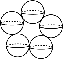
Figure 2.3: The toroidal fibre at an $A_{4}$ singularity. The torus is “pinched” in five places so that it becomes a necklace of five two-spheres joined at points.

2.4.2 Connection to physics

This ADE classification of the fibration (2.9) is a purely mathematical result, but due to the interpretation of the torus modulus $\tau$ as a coupling constant, it has inspired a line of physics investigations that has proved very fruitful. The idea is that each of the singularities listed above corresponds to a four-dimensional ${\cal N}$=2 SYM theory with global symmetry corresponding to the singularity type. In particular, the interesting theories are the ones at strong coupling, i.e. at the seven singularities at finite $\tau$ (Im $\tau=\infty$ corresponds to weak coupling).

For instance, the original Seiberg-Witten theory, i.e. ${\cal N}$=2 SYM with $SU(2)$ gauge group and four hypermultiplets (which has $SO(8,{{\mathbb{C}}\,})$ global symmetry), fits nicely in this picture as the strongly coupled theory at the $D_{4}$ singularity. The $A_{0}$, $A_{1}$ and $A_{2}$ theories (i.e. they have global symmetries $SL(1,{{\mathbb{C}}\,})$, $SL(2,{{\mathbb{C}}\,})$ and $SL(3,{{\mathbb{C}}\,})$) are obtained as certain limits of an $SU(2)$ gauge theory with respectively one, two and three hypermultiplets [23, 24]; these theories can be derived from the $D_{4}$ theory.

The success of this correspondence thus far then prompted the corresponding computation for the $E_{6}$, $E_{7}$ and $E_{8}$ theories, i.e. theories with exceptional global symmetries [25, 26, 27]. The existence of such SW-theories has been shown also via compactifications of higher-dimensional gauge theories [28]. The computation of exceptional varieties is explained in detail in e.g. [29].

2.4.3 Brane picture

The picture of the coupling constant as a torus parameter has given rise to the idea of F-theory [30]. This is a conjectured twelve-dimensional theory which, when compactified on a four-dimensional K3 manifold, is equivalent to Type IIB theory compactified on a two-dimensional manifold such as a sphere or a two-torus. The K3 manifold is a fibration of tori over the two-dimensional manifold, and the coupling constant $\tau$ parameterises the fibre tori.

To see how this picture is relevant to us, we need to go into some detail. Take the two-dimensional base space to be ${\mathbb{P}}^{1}$, parameterised by the complex coordinate $z$. Then the K3 manifold is described by an algebraic variety of the form (2.9) with $f$ and $g$ being of degree eight and twelve respectively in $z$, and it has 24 singularities. These are determined as the zeroes of the discriminant of the variety [21], and correspond in the IIB picture to the positions on ${\mathbb{P}}^{1}$ of 24 spacefilling 7-branes (filling up the eight uncompactified dimensions) [31].

When a specific combination of $(p,q)$ 7-branes (i.e. 7-branes on which $(p,q)$-strings can end) coincide at a particular value of $\tau$, or equivalently, at a particular point on ${\mathbb{P}}^{1}$, then the gauge symmetry on the worldvolume of these 7-branes is enhanced. Which particular gauge group we get depends on the number and types of 7-branes involved [31, 32]; the different possibilities include the ADE groups and were categorised in [27].

Next we do what Banks et al [33] did and introduce a D3-brane parallel to the 7-branes and located close to their position in ${\mathbb{P}}^{1}$. This “probe technique” is a popular approach to studying the properties of string theory backgrounds; by “probe” we mean that the D3-brane does not itself affect the background geometry. This is admittedly an approximation, and backreaction has been taken into account in e.g. [34, 35].

The probe provides an alternative picture of some of the physics on the 7-branes, as features of the worldvolume theory living on the D3-brane. This is a four-dimensional ${\cal N}$=2 SYM theory with a broken gauge symmetry that becomes enhanced at the singularity. Here it also becomes superconformal, and acquires a global symmetry which is the same as the gauge symmetry on the 7-branes [33, 36]. Moreover, the hypermultiplet fields are strings stretched between the D3-brane and the various 7-branes, whereas the vector multiplets correspond to strings with both ends on the D3-brane.

We have thus constructed a somewhat elaborate string theory setup in order to obtain a brane interpretation of the globally symmetric, superconformal theory. But it was worth the effort; we now have a clear picture of the generalised Coulomb branch in terms of F-theory — it is just the K3 manifold on which the twelve-dimensional theory is compactified (the ordinary Coulomb branch of the probe is the base space ${\mathbb{P}}^{1}$). In particular this has made it possible to find the exact moduli space for strongly coupled SW-theories [25, 26, 27].

Moreover, this setup is relevant here because now we have brane pictures for both of the two gauge theories that Paper I relates to. The other theory, the quiver gauge theory, which has a more straightforward brane interpretation, is discussed in the next section. But first we remark that since, as was shown in [8, 9] and Paper I, there is a nontrivial identity between the moduli spaces of these two different theories, we expect there to be some kind of duality between the two string theory backgrounds. However, this turns out to be less than manifest, and attempts at finding such a duality have failed thus far (see e.g. [37]).

Let us now explain what we mean by a quiver theory.

2.5 Quiver gauge theory

Quiver gauge theory is a well-established concept that frequently crops up in string theory [14, 38]. At first sight this type of theory may seem anything but natural, as it involves a rather specific gauge structure — a product of unitary groups and matter fields transforming according to a strict pattern as bifundamentals under pairs of the constituent gauge groups. However, in the quest for realistic physics based on string theory one must break both supersymmetry and gauge symmetry in some way, and one of the most straightforward procedures yields precisely what we call quiver theory.

The idea is to start with Type IIB string theory in ten flat dimensions (coordinates $x^{0},x^{1},...,x^{9}$) and introduce a stack of $N$ coinciding D3-branes. We arrange these branes such that their four-dimensional worldvolumes are aligned with the 0-1-2-3-directions $x^{0},...,x^{3}$. The worldvolume supports a pure ${\cal N}$=$4$ SYM theory, i.e. the only matter present is a vector multiplet containing three complex (= six real) scalar fields transforming in the adjoint representation of the gauge group. In the string theory picture these scalars are the coordinates of the position of the branes along the six dimensions transverse to the branes. As long as they all coincide, the gauge symmetry is $U(N)$; this is due to the way in which the ends of open strings are indexed (by Chan-Paton indices) according to which branes in the stack they are attached to (see [39], Section 6.5).

However, if the branes separate from each other, the gauge group is broken down to some subgroup, since there will be fewer branes for massless strings to end on. This is precisely the Higgs mechanism from the point of view of the gauge theory; moving the branes corresponds to giving expectation values to the scalar fields, which breaks the gauge symmetry.

To break supersymmetry we make an orbifold out of the 6-7-8-9-dimensions by imposing an identification on the coordinates under a group $\Gamma$. That is, two points are considered identical if they differ only by a $\Gamma$-transformation. Note that the origin $x^{\mu}=0$ is fixed under $\Gamma$-transformations — this is the orbifold singularity, which will be blown up later.

Here we choose $\Gamma$ to be a discrete subgroup of $SU(2)$; the motivation for this is that the resulting orbifold ${{\mathbb{C}}\,}^{2}/\Gamma$ follows the same ADE classification as a K3 surface, and may be viewed as a local description of a K3 singularity, at least near the origin. As will become clear presently, this orbifold constitutes the Higgs branch of the worldvolume theory, and as we mentioned in Section 2.3 it is required by ${\cal N}$=2 supersymmetry to be just such an orbifold.

To summarise, we have the following configuration,

$$\begin{array}[]{|c|c|c|c|c|c|c||c|c|c|c|}\hline\cr\textstyle{\mathrm{Spacetime}}\,\,\textstyle{\mathrm{directions}}&0&1&2&3&4&5&6&7&8&9\\ \hline\cr|\Gamma|\,\,\,\textstyle{\mathrm{D3-branes}}&\times&\times&\times&\times&\cdot&\cdot&\cdot&\cdot&\cdot&\cdot\\ \hline\cr\textstyle{\mathrm{Orbifold}}\,\,\,{{\mathbb{C}}\,}^{2}/\Gamma&&&&&&&\times&\times&\times&\times\\ \hline\cr\end{array}$$

where crosses indicate the dimensions along which the brane or orbifold extends, and a dot means the brane is pointlike in that direction.

We now explore the consequences of the $\Gamma$-identification.

2.5.1 Effects of orbifolding

When we perform the orbifolding, the $U(N)$ gauge group breaks down to a product of unitary groups, which we call $F$. One of the ${\cal N}$=$4$ complex scalars remains in the adjoint representation of the broken gauge group. The other two scalars on the other hand transform as bifundamentals according to a special pattern. This rearrangement of the matter fields breaks the supersymmetry down to ${\cal N}$=2; the adjoint scalar becomes the scalar in the ${\cal N}$=2 vector multiplet, while the two bifundamentals constitute the scalars of two hypermultiplets. Thus the worldvolume theory on the branes is now an ${\cal N}$=2 SYM theory with two hypermultiplets.

It is easy to see explicitly how the orbifolding acts on the gauge group and the scalars. A detailed account of the orbifolding procedure is given in [14], and we merely sketch it here. The fields that we are interested in, namely the vector fields $A^{a}_{\mu}$ ($a$ labels the gauge group generators), the complex 4-5-coordinate $\varphi\equiv x^{4}+ix^{5}$, and the complex 6-7-8-9-coordinates $\phi^{1}\equiv x^{6}+ix^{7}$ and $\phi^{2}\equiv x^{8}+ix^{9}$, all arise as massless excitations of open strings. We can therefore represent them by matrices encoding their Chan-Paton indices. With $N$ branes present, these matrices have dimension $N\times N$ with, in a suitable basis, the ($i$,$j$) entry specifying whether or not the string stretches between the $i$:th and $j$:th branes.

Here we take the number of branes to equal the order of the orbifold group, $N=|\Gamma|$. Although the reason for this choice will become clear later, we attempt to justify it already at this point. Our aim is to represent the action of $\Gamma$ on the open string sector, and since there are $|\Gamma|$ distinct elements of the orbifold group, we need $|\Gamma|$ different string states to represent them. Therefore the strings need to be able to end on $|\Gamma|$ different branes; these string states provide a faithful representation of $\Gamma$.

We use the following notation for the Chan-Paton matrices,

$$A^{a}_{\mu} \rightarrow \lambda^{a}_{V},$$ (2.11)

$$\varphi \rightarrow \lambda_{I},$$ (2.12)

$$\phi^{1} \rightarrow \lambda^{1}_{II},$$ (2.13)

$$\phi^{2} \rightarrow \lambda^{2}_{II}.$$ (2.14)

In the unorbifolded theory, all these fields belong to the vector multiplet and therefore transform in the adjoint representation of the unbroken gauge group $U(|\Gamma|)$. However, the requirement that they be invariant under the orbifold group $\Gamma$ imposes restrictions on the Chan-Paton matrices such that this is no longer true.

If we denote by $\gamma_{\Gamma}$ the regular matrix representation of $\Gamma$, then a field is $\Gamma$-invariant if it commutes with $\gamma_{\Gamma}$. We therefore impose

$$\lambda^{a}_{V} = \gamma_{\Gamma}\lambda^{a}_{V}\gamma^{-1}_{\Gamma},$$ (2.15)

$$\lambda_{I} = \gamma_{\Gamma}\lambda_{I}\gamma^{-1}_{\Gamma}.$$ (2.16)

For $\phi^{1,2}$, however, we need to take into account the fact that they live along the orbifold directions. This means that the invariance condition involves an extra $\Gamma$-action on the doublet ($\phi^{1}$, $\phi^{2}$), via the 2$\times$2 matrix representation acting on the quaternion (2.8). We call this matrix $G_{\Gamma}$, and find the following invariance condition for $\phi^{i}$,

$$\lambda^{i}_{II}=\left(G_{\Gamma}\right)^{i}_{\,\,j}\gamma_{\Gamma}\lambda^{j}_{II}\gamma^{-1}_{\Gamma}.$$ (2.17)

It is now a matter of straightforward matrix algebra to derive the form of the Chan-Paton matrices that satisfy Eqs. (2.15)–(2.17), and the result is the aforementioned factorisation of the gauge group and the bifundamental structure. Some explicit such calculations are shown in e.g. [37].

Note that the vacuum moduli space now consists of two branches, as expected of a four-dimensional ${\cal N}$=2 theory. The 4-5-space, induced by the vector multiplet $\varphi$, constitutes the Coulomb branch, and the orbifolded 6-7-8-9-space, induced by the hypermultiplets $\phi^{i}$, is the Higgs branch.

So what about the Fayet-Iliopoulos terms? To find the corresponding object in the string theory picture it is not sufficient to look only at the open string sector. We need to include massless closed strings, in particular the twisted ones. That is, string states that are invariant under the orbifold group only as long as they stay at the singularity. These states enter the worldvolume theory of the D3-branes in exactly the same way as FI-terms [14].

2.5.2 Quiver diagrams

The resulting gauge structure has the interesting feature that it falls into an ADE classification. That is, one may use the ADE (extended) Dynkin diagrams to encode the transformation properties of the bifundamentals. As explained above, these properties are directly related to the group $\Gamma$. For instance, $\Gamma={\mathbb{Z}}_{n}$ breaks the gauge group down to a direct product of $n$ $U(1)$’s and arranges the hypermultiplets to transform as ($\mathbf{1}$, $\mathbf{\bar{1}}$) under pairs of $U(1)$’s according to an $A_{n-1}$ pattern.

That is, we may represent the gauge structure by means of an $A_{n-1}$ extended Dynkin diagram, as shown in Fig. 2.4. The nodes of the diagram each corresponds to a $U(1)$ factor (i.e. a FI-term) and the edges describe the bifundamentals with the arrow pointing towards the antifundamental representation. Similarly, for $\Gamma$ equal to the dihedral group ${\cal D}_{n}$, we obtain a $D_{n-2}$ structure, and $\Gamma={\cal T}$, the tetrahedral group, yields an $E_{6}$ structure. The octahedral group, $\Gamma={\cal O}$, gives $E_{7}$, and the icosahedral $\Gamma={\cal I}$ an $E_{8}$ structure. Thus there is a one-to-one correspondence between the discrete groups $\Gamma$ and the ADE Lie algebras.

Figure 2.4: The $A_{n-1}$ quiver diagram associated with the ${\mathbb{Z}}_{n}$ orbifold group. The “1” in each node refers to the corresponding $U(1)$ factor in the quiver gauge group $U(1)^{n}$, and the arrows indicate the transformation properties of the bifundamentals. In this context the $\alpha_{i}$’s denote FI-parameters.

That the quiver diagrams are extended Dynkin diagrams means that there is an extra $U(1)$ node compared to the ordinary Dynkin diagram. This extra $U(1)$ factor comes from the fact that there is a trivial solution of (2.15), namely $\lambda^{0}_{V}=\hbox{11}$, the identity matrix; the trivial solution corresponds to a $U(1)$ that will always remain unbroken no matter what we do to the branes. In terms of the worldvolume gauge theory this means we can Higgs away all the vector multiplets except the one corresponding to the trivial $U(1)$. This $U(1)$ group is the gauge group in the worldvolume theory of a single D-brane, so we see that the hypermultiplets now parameterise the position in the orbifold of a single D3-brane. From the point of view of the covering space ${{\mathbb{C}}\,}^{2}$, this brane is actually a stack of $|\Gamma|$ fractional branes, moving simultaneously in such a way that they are images of each other under $\Gamma$.

2.6 The ${\cal N}$=2 Higgs branch

The object of Paper I was to show that the Higgs branch of the $E_{8}$ quiver theory is identical to the generalised Coulomb branch of $E_{8}$ Seiberg-Witten theory. There is no problem to do this in the singular limit; then the quiver Higgs branch is just the orbifold ${{\mathbb{C}}\,}^{2}/{\cal I}$, which is described essentially by Eq. (2.9) with $f(z)=0$ and $g(z)=z^{5}$.

The subtle difference is that the variables $x$, $y$ and $z$ are $F$-invariants here, not ${\cal I}$-invariants, although they are isomorphic to the latter [40]. To make the distinction explicit, we call the $F$-invariants $X$, $Y$ and $Z$, and find the variety [8]

$$Y^{2}+X^{3}+Z^{5}=0$$

for the $E_{8}$ quiver Higgs branch.

For nonsingular moduli spaces matters are more involved. We already know the algebraic variety for the resolved SW-theory — it is Eq. (2.9), with [27]

$$f(z) = w_{2}z^{3}+w_{8}z^{2}+w_{14}z+w_{20}$$ (2.18)

$$g(z) = z^{5}+w_{12}z^{3}+w_{18}z^{2}+w_{24}z+w_{30}.$$ (2.19)

Here the coefficients $w_{n}$ are deformation parameters; when they are nonzero, the singularity is deformed so that the space becomes smooth.

However, we did not know the explicit form of the resolved quiver Higgs branch (the ALE space), so we computed it in Paper I, in terms of FI-parameters. The resulting variety was then brought, by means of variable substitutions, to the form (2.9) with $f$ and $g$ given by (2.18) and (2.19), except the coefficients in $f$ and $g$, which we called $\omega_{n}$, were now explicit polynomials in FI-terms. These polynomials may a priori be different from the deformation parameters of the SW-theory, and the conclusion in Paper I was that they are in fact identical.

Before concluding this chapter, we briefly remark on the details of the Higgs branch computation and comparison to the SW-variety.

2.6.1 Comparing the moduli spaces

To compute the Higgs branch we used so-called “bug calculus,” introduced in [8] and reviewed in [41]. It is essentially a technique to avoid writing zillions of indices in computations that involve a lot of fields. Polynomials in the ADE bifundamentals are represented by lines drawn in quiver diagrams, and traces (invariants) correspond to closed loops. These loops may then be manipulated subject to a set of constraints that reflect the D-flatness conditions (i.e. the moment map constraints), and we thus find the algebraic variety for the quiver Higgs branch.

The comparison between the $E_{8}$ quiver Higgs branch and the $E_{8}$ SW-variety boils down to showing that our coefficients $\omega_{n}$ are equal to the deformation parameters $w_{n}$ of Noguchi et al [27]. The link between the two notations goes via the simple roots. To see how, we introduce the characteristic polynomial,

$$P^{{\cal R}}_{G}\equiv\det(t\hbox{11}-v\cdot H)=\prod^{\dim{\cal R}}_{k=1}(t-v_{k}),$$

where ${\cal R}$ is some representation of the group $G$, $t$ is a complex parameter, and $v_{k}$ are the weights of the representation ${\cal R}$. The matrix $v\cdot H\equiv\textstyle{\mathrm{diag}}(v_{k})$ is the matrix with the weights on the diagonal and zeros otherwise, and 11 is the identity matrix. The vanishing of $P^{{\cal R}}_{G}$ encodes the same information about the singularity in an elliptic fibration as the hypersurface (2.9) [18].

In particular, it is convenient to use the characteristic polynomial for computing the Casimir invariants of $G$, and this is what Noguchi et al [27] did to express the $E_{8}$ Casimir invariants (= elements of $E_{8}$ that commute with all generators) in terms of the deformation parameters $w_{n}$. Their equations are easily inverted so as to express the $w_{n}$’s in terms of Casimirs, which in turn are polynomials in the weights $v_{k}$. And since the weights may be written in terms of the simple roots as shown in Section 2.2, we obtain the Casimirs as polynomials in the simple roots. We thus have the $w_{n}$’s expressed in terms of FI-parameters, hence they may be explicitly compared with our coefficients $\omega_{n}$ (which were defined as polynomials in FI-terms already from the beginning).

Chapter 3 Boundary conditions

3.1 Introduction

This chapter is concerned with the dynamics of the ends of open superstrings. As an open string propagates through spacetime it sweeps out a two-dimensional worldsheet. The ends of the string trace out one-dimensional paths, which constitute boundaries of the worldsheet. The motion of the string, and hence the shape of its worldsheet, is dictated by equations of motion derived from a two-dimensional field theory called the nonlinear sigma model. It is an action integral whose domain is the worldsheet, parameterised by two coordinates: $\sigma$ along the string, and a time coordinate $\tau$ along the direction of motion. The target space of this integral is spacetime; that is, the dynamical fields in the action are the vectors $X^{\mu}(\tau,\sigma)$, giving the position in spacetime of the worldsheet point $(\tau,\sigma)$. Thus the dynamics of the string is described by the equations of motion for $X^{\mu}$.

In particular, the end of the string moves according to the equations of motion on the domain boundary (boundary conditions), which restrict it to move on some hypersurface in spacetime. Since open strings are by definition attached to D-branes, this hypersurface is a D-brane. Thus, in defining the hypersurface where the end is allowed to move, the boundary equations of motion are telling us what the corresponding D-brane looks like, see Fig. 3.1.

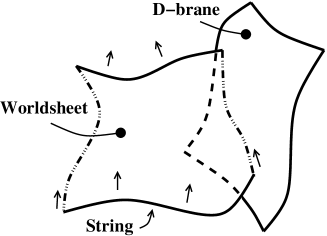
Figure 3.1: An open string propagating in spacetime sweeps out a two-dimensional worldsheet. The hypersurface to which its end is confined defines a D-brane.

How restrictive these equations of motion are depends on the amount of symmetry preserved on the boundary. We focus here on the minimally (${\cal N}$=1) supersymmetric conformal nonlinear sigma model, assuming that the worldsheet bulk superconformal symmetry is preserved also on the boundary (the D-brane). We showed in Papers II–IV that the boundary conditions allowed by this assumption are more general than those commonly used elsewhere — the latter conditions are just special cases. Nevertheless, we will see that our conditions do impose some restrictions on the properties of D-branes.

In deriving the boundary equations of motion, the naive approach would be to do so directly from the action, by use of the principle of least action (i.e. a perturbation of the action should vanish). This is hazardous, as the result does not necessarily preserve the desired symmetries. One could in principle amend this by modifying the action by extra boundary terms to make it superconformal on the boundary. However, there is no systematic way to find those boundary terms, except guessing them. In Papers II and III we therefore went for the safer method of analysing the currents that correspond to the relevant symmetries, requiring that they be conserved on the boundary. This defines boundary conditions for the currents, from which we could derive conditions on the brane.

Having thus obtained the minimal requirements for boundary superconformal invariance in a general background, it is natural to consider a special case of background. In Paper IV we chose the ever popular WZW model, which is a nonlinear sigma model defined on a group manifold, with chiral isometry currents [44, 45]. Here our boundary conditions imply a surprisingly general gluing map between the isometry currents, the geometrical implications of which remain unclear at the time of writing.

3.1.1 Outline

To introduce some fundamental concepts pertaining to symmetries and conserved currents, we begin in Section 3.2 by discussing the bosonic nonlinear sigma model. Then we define the supersymmetric sigma model in Section 3.3, explaining about superspace and superfields, and how to derive the superconformal currents. In Section 3.4 we make an ansatz for the worldsheet fields which, after introducing some necessary notation in Section 3.5, we plug into the conservation laws for the currents and obtain in Section 3.6 the complete set of conditions for a superconformal D-brane, which we interpret in geometrical terms. Prompted by similarities to the structures of almost product manifolds, we look at globally defined boundary conditions in Section 3.7, drawing some conclusions about the global embedding of D-branes in spacetime. Finally in Section 3.8 we apply our analysis to the WZW model, leading to some interesting statements about gluing maps of group currents.

3.2 The bosonic model

Consider an open string of tension $T$ propagating on a spacetime manifold that supports a general background two-tensor $E_{\mu\nu}(X)\equiv G_{\mu\nu}(X)+B_{\mu\nu}(X)$. Here $G_{\mu\nu}$ is the spacetime metric and $B_{\mu\nu}$ an antisymmetric B-field, both of which may depend on the spacetime coordinates $X^{\mu}$. Then the nonlinear sigma model for the string is (see [46], Section 3.4)

$$S = -\frac{T}{2}\int d\tau d\sigma\,\left[\,\sqrt{-g}\,g^{ab}\partial_{a}X^{\mu}\partial_{b}X^{\nu}G_{\mu\nu}(X)\right.$$ (3.1)

$$\left.+\,\epsilon^{ab}\partial_{a}X^{\mu}\partial_{b}X^{\nu}B_{\mu\nu}(X)\,\right],$$

where $g_{ab}$ is the metric on the worldsheet, $g\equiv\det g_{ab}$, and $\epsilon^{ab}$ is the worldsheet antisymmetric tensor with $\epsilon^{\tau\sigma}$=$-\epsilon^{\sigma\tau}$=1 and $\epsilon^{\tau\tau}=\epsilon^{\sigma\sigma}$=0.

One may derive equations of motion for the string by varying (3.1) with respect to $X^{\mu}$. Since the string is open, the domain of the integral has boundaries, which contribute boundary terms to the equations of motion. The dynamics of the ends of the string is then determined by the vanishing of these boundary terms, implying some nontrivial boundary conditions for the open string.

The boundary conditions are of two types; either the string is moving freely along the $X^{\mu}$-direction — Neumann conditions — or it is stuck in that direction — Dirichlet conditions. The hypersurface to which the string’s endpoint is confined, i.e. the D-brane, thus extends along Neumann directions and is pointlike in Dirichlet directions (see [39], Chapter 8).

However, the boundary equations of motion obtained in this way do not necessarily preserve all the symmetries that are preserved in the bulk. If our prime concern is that they do (which it is), then we are better off analysing conserved currents.

3.2.1 Conserved currents

The model (3.1) is invariant under three different symmetries: spacetime Poincaré transformations, worldsheet conformal transformations (rescaling of the two-dimensional metric $g_{ab}$), and worldsheet reparameterisation. The last symmetry allows us to switch to lightcone coordinates on the worldsheet, $\xi^{\pm}\equiv\tau\pm\sigma$, and we use this basis henceforth.

Each symmetry corresponds to a conserved current, obtained by varying the action with respect to the appropriate field. The requirement that the action be invariant under this perturbation (in the bulk) translates into a conservation law saying that the current is divergence-free, i.e. there are no sources. For example in the case of conformal invariance, the corresponding current is the stress energy-momentum tensor and is derived by varying (3.1) with respect to $g_{ab}$. Its components in lightcone coordinates are

$$T_{\pm\pm}=\partial_{\mbox{\tiny${}_{\stackrel{{\scriptstyle{+\!\!\!+}}}{{=}}}$}}X^{\mu}\partial_{\mbox{\tiny${}_{\stackrel{{\scriptstyle{+\!\!\!+}}}{{=}}}$}}X^{\nu}G_{\mu\nu},$$ (3.2)

where $\partial_{\mbox{\tiny${}_{\stackrel{{\scriptstyle{+\!\!\!+}}}{{=}}}$}}$ are the derivatives with respect to $\xi^{\pm}$, and we have rescaled the tension to one. The $T_{++}$ component depends only on $\xi^{+}$, and is called the “left-moving” current, whereas $T_{--}$ depends only on $\xi^{-}$ and is referred to as “right-moving.” Here the bulk conservation law takes the form $\partial_{=}T_{++}=\partial_{{+\!\!\!+}}T_{--}=0$.

To ensure that also the boundary is conformally invariant, we need to impose current conservation on the boundary separately. In general we find the boundary condition for a given current $J^{a}_{\,\,\,b}$ by using its associated charge $Q_{b}\equiv\int d\sigma J^{\tau}_{\,\,\,b}$. This charge is conserved in the sense that it is time-independent, $\partial_{\tau}Q_{b}=0$ (see [11], Section 3.2). Thus, since $J^{a}_{\,\,\,b}$ obeys the conservation law $\partial_{a}J^{a}_{\,\,\,b}=0$, we may write charge conservation as

$$0=\partial_{\tau}Q_{b}=\int d\sigma\,\,\,\partial_{\tau}J^{\tau}_{\,\,\,b}=-\int d\sigma\,\,\,\partial_{\sigma}J^{\sigma}_{\,\,\,b}=-[\,J^{\sigma}_{\,\,\,b}\,]^{\sigma=\pi}_{\sigma=0}.$$ (3.3)

Hence we obtain the boundary condition $J^{\sigma}_{\,\,\,b}=0$, for $b=\tau,\sigma$. Applied to the stress tensor, the result is

$$T_{++}-T_{--}=0,$$ (3.4)

i.e. the left- and right-moving components of the stress tensor must be equal. Via the relation (3.2) between the stress tensor and the worldsheet fields, we thus find a boundary condition relating the left-moving fields $\partial_{{+\!\!\!+}}X^{\mu}$ to the right-moving fields $\partial_{=}X^{\mu}$.

In conclusion, we have derived the condition for conformal invariance on the boundary in the bosonic model. But we are interested in the supersymmetric theory, which looks a little bit different.

3.3 The superspace action

The bosonic model (3.1) has only the three symmetries listed in Section 3.2. If we want more symmetry the action needs to be modified. In particular, to make it supersymmetric we have to add superpartner fields that together with the bosonic worldsheet scalars $X^{\mu}$ make up multiplets (cf. Section 2.3). We thus add two worldsheet spinors $\psi^{\mu}_{\pm}$ and an auxiliary (i.e. nondynamical) field $F^{\mu}_{+-}$.

The fields constituting a multiplet can be conveniently collected in a single superfield. The idea is to promote the ordinary worldsheet to a superspace by supplementing the bosonic worldsheet coordinates $\xi^{\pm}$ with anticommuting coordinates $\theta^{\pm}$. Superfields are terminating polynomials in $\theta^{\pm}$, with the multiplet fields as coefficients. For example, a multiplet ($X^{\mu}$, $\psi^{\mu}_{\pm}$, $F^{\mu}_{+-}$) would correspond to the superfield [15]

$$\Phi^{\mu}\equiv X^{\mu}+i\theta^{+}\psi^{\mu}_{+}+i\theta^{-}\psi^{\mu}_{-}+\theta^{+}\theta^{-}F^{\mu}_{+-}.$$

Similarly, the worldsheet derivatives $\partial_{\mbox{\tiny${}_{\stackrel{{\scriptstyle{+\!\!\!+}}}{{=}}}$}}$ in (the lightcone version of) (3.1) are extended by additional “superderivatives” $D_{\pm}$, and the action becomes an integral over superspace rather than over ordinary space. Superspace comes equipped with integration rules that render this integral equivalent to the ordinary one [15].

The whole point of using superfield notation is that the supersymmetric theory can be analysed in a much more compact way than if we were to use the explicit “component form.” Instead of writing out the kinetic terms in the action for all the multiplet fields individually, we can simply replace the bosonic fields in (3.1) with superfields. In lightcone coordinates we thus obtain

$$S=\int d^{2}\xi d^{2}\theta D_{+}\Phi^{\mu}D_{-}\Phi^{\nu}{{\cal E}}_{\mu\nu}(\Phi),$$ (3.5)

where ${{\cal E}}_{\mu\nu}$ is the superfield whose lowest component is the background tensor $E_{\mu\nu}$. Analysis of the superspace action can then be performed in a way completely analogous to the bosonic case, using superspace quantities instead of bosonic ones.

Without boundaries, the action (3.5) is ${\cal N}$=(1,1) (globally) supersymmetric, i.e. it is invariant under two independent supersymmetry transformations that transform the bosonic and fermionic fields into each other. One is parameterised by a left-moving supersymmetry parameter $\varepsilon^{+}$, and the other by a right-moving one, $\varepsilon^{-}$. These two parameters are a priori independent of each other, and each of them is associated with a conserved supersymmetry current; we denote these currents by $G_{\pm}$.

In the presence of a boundary the supersymmetry parameters and currents are subject to boundary conditions that relate left- and right-movers, as we saw in Section 3.2. The supersymmetry parameters become identified up to a sign, $\varepsilon^{+}=\eta\varepsilon^{-}$ ($\eta\equiv\pm 1$), reducing the ${\cal N}$=(1,1) symmetry to ${\cal N}$=1. For the currents the boundary condition (3.3) is

$$G_{+}-\eta G_{-}=0,$$ (3.6)

which is the condition for the boundary to preserve worldsheet supersymmetry.

The condition (3.6) together with the stress tensor condition (3.4) define the superconformal boundary conditions for the classical open superstring. It is these two conditions that served as our starting point in Papers II–IV. To derive the corresponding boundary conditions for the worldsheet fields we need to write the currents $T_{\pm\pm}$ and $G_{\pm}$ in terms of $X^{\mu}$ and $\psi^{\mu}_{\pm}$. In the bosonic theory the expression for the stress tensor was (3.2); here the relation is more complicated, involving also $\psi^{\mu}_{\pm}$. We now briefly explain how to compute the superconformal currents from a locally supersymmetric sigma model.

3.3.1 Finding the currents

The conformal and supersymmetry currents can be viewed as components of a superfield which we call the “supercurrent,” and which we denote by $T_{A}^{\,\,\,B}$ (the indices $A,B$ run over the superspace indices ${+\!\!\!+},=,+,-$). This is a kind of stress tensor for a locally supersymmetric version of the nonlinear sigma model (3.5).

What one does is to “gauge” the model by replacing the flat superderivatives $D_{\pm}$ with covariant ones, $\nabla_{\pm}$, as well as introducing a supervielbein $\mathfrak{E}_{M}^{\,\,\,A}$ on superspace (see [46], Section 4.3.4). The action then becomes

$$S=\int d^{2}\xi d^{2}\theta\,\,\mathfrak{E}\,\,\nabla_{+}\Phi^{\mu}\,\nabla_{-}\Phi^{\nu}\,{{\cal E}}_{\mu\nu}(\Phi),$$

where $\mathfrak{E}$ is the determinant of the supervielbein.

Next we vary $S$ with respect to the vielbein components and obtain the supercurrent, of which only two components do not vanish on-shell, namely $T^{\,\,\,-}_{{+\!\!\!+}}$ and $T^{\,\,\,+}_{=}$ [48]. These are expressions in covariant superderivatives of superfields, and we revert to global supersymmetry by replacing the covariant derivatives with flat ones again. Finally, we can extract the components of the supercurrent as follows,

$$G_{+}=T_{{+\!\!\!+}}^{\,\,\,-}|,\quad\quad G_{-}=T_{=}^{\,\,\,+}|,$$

$$T_{++}=-iD_{+}T_{{+\!\!\!+}}^{\,\,\,-}|,\quad\quad T_{--}=-iD_{-}T_{=}^{\,\,\,+}|.$$

The result is a set of explicit expressions for the currents in terms of worldsheet fields, which we omit here; they are given in Paper III.

It is now in principle straightforward to convert the boundary conditions (3.4) and (3.6) for the currents into boundary conditions for the fields $X^{\mu}$ and $\psi^{\mu}_{\pm}$. We know that the boundary enforces relations between left- and right-movers, so we can make an ansatz for the way in which the left- and right-moving worldsheet fields are related to each other, and then derive restrictions on this ansatz from the current conditions. Thus our plan of attack is to make the most general ansatz possible for the worldsheet fields, plug it into the current conditions, and reduce these conditions to an independent set of boundary conditions that we can interpret.

3.4 The ansatz

It turns out that the most general, local ansatz we can make in our classical conformal theory is very simple for the fermions, due to the absence of dimensionful parameters. We therefore start with this ansatz and then derive the corresponding bosonic relation by a supersymmetry transformation. A little dimensional analysis reveals that the fermionic ansatz takes the form (the sign $\eta=\pm 1$ is included merely for convenience)

$$\psi_{-}^{\mu}=\eta R^{\mu}_{\,\,\nu}(X)\,\psi_{+}^{\nu},$$ (3.7)

where $R^{\mu}_{\,\,\nu}$ is a general (1,1)-tensor defined on the boundary, which may depend on the worldsheet scalar $X^{\mu}$ at that point, but not on $\psi_{\pm}^{\mu}$. The bosonic superpartner of (3.7) is more complicated,

$$\partial_{=}X^{\mu}-R^{\mu}_{\,\,\nu}\partial_{+\!\!\!+}X^{\nu}+2i(P^{\sigma}_{\,\,\rho}\nabla_{\sigma}R^{\mu}_{\,\,\nu}+P^{\mu}_{\,\,\gamma}G^{\gamma\delta}H_{\delta\sigma\rho}R^{\sigma}_{\,\,\nu})\psi_{+}^{\rho}\psi_{+}^{\nu}=0,$$ (3.8)

where we have defined $2P^{\mu}_{\,\,\nu}\equiv\delta^{\mu}_{\,\,\nu}+R^{\mu}_{\,\,\nu}$ ($\delta^{\mu}_{\,\,\nu}$ is the Kronecker delta), the antisymmetric three-tensor $H_{\mu\nu\rho}$ is the field strength (or torsion) of the background B-field, and $\nabla_{\sigma}$ is the Levi-Civita connection. Note that (3.8) is more general than the usual boundary conditions adopted in the literature (see e.g. [49]), in that there is an extra two-fermion term allowed by superconformal invariance. We showed in Papers II and III that this extra term vanishes only for very special cases.

The ansatz (3.7) encodes in a covariant form the standard Neumann and Dirichlet boundary conditions that define a D-brane. In the presence of a B-field the Neumann condition has an a priori very general form, while the Dirichlet condition is much simpler. If we choose a basis where the worldvolume coordinates of the D-brane are aligned with the spacetime coordinates — called adapted coordinates — then the Dirichlet condition takes the familiar form

$$\partial_{\tau}X^{i}=0,$$ (3.9)

stating that the position of the endpoint along the $i$:th Dirichlet direction does not change with worldsheet time $\tau$, i.e. it is frozen in that direction. The corresponding situation holds for the spinors,

$$\psi_{-}^{i}=-\eta\,\psi_{+}^{i}.$$ (3.10)

At first glance $R^{\mu}_{\,\,\nu}$ seems a completely general object, but we can actually say something about it already at this stage, by going to adapted coordinates at a point. In this basis it should imply (3.10), so the Dirichlet-Dirichlet part is $R^{i}_{\,\,j}=-\delta^{i}_{\,\,j}$. On the other hand, the Neumann condition is still very general ($m,n$ label Neumann directions),

$$\psi_{-}^{m}=\eta R^{m}_{\,\,n}(X)\,\psi_{+}^{n},$$ (3.11)

for some Neumann-Neumann tensor $R^{m}_{\,\,n}$. It is clear that this tensor depends on the B-field, because for $B_{\mu\nu}=0$ we expect (3.11) to reduce to $\psi_{-}^{m}=\eta\,\psi_{+}^{m}$. In fact, one may think of $R^{m}_{\,\,n}$ as defining the B-field; we will see later precisely how.

To summarise, if we write $R^{\mu}_{\,\,\nu}$ as a 2$\times$2 block matrix, with the upper left block being the Neumann-Neumann part, the lower right the Dirichlet-Dirichlet part, and the off-diagonal blocks the mixed parts, we have

$$R^{\mu}_{\,\,\nu}=\left(\begin{array}[]{cc}R^{m}_{\,\,n}&0\\ 0&-\delta^{i}_{\,\,j}\end{array}\right).$$ (3.12)

But we want to work in a basis-independent notation, so we would like to write for example the Dirichlet condition (3.9) in a covariant form. To do this, we need to introduce some structures on our spacetime manifold. These structures are natural from a physical point of view, but there is a rich mathematical machinery associated with them, which will be tremendously useful in writing down and interpreting the final boundary conditions.

3.5 Structures on D-branes

We begin by defining a projector $Q^{\mu}_{\,\,\nu}$ on the worldsheet boundary, which projects vectors on the D-brane onto the space spanned by the Dirichlet directions. That is, given a vector $X^{\mu}$ at some point on the brane, $Q^{\mu}_{\,\,\nu}X^{\nu}$ is by definition normal to the brane at that point. If $X^{\mu}$ is invariant under $Q^{\mu}_{\,\,\nu}$, $Q^{\mu}_{\,\,\nu}X^{\nu}=X^{\mu}$, then it is a pure Dirichlet vector. In this sense, $Q^{\mu}_{\,\,\nu}$ assigns a vector space to each point $u$ on the brane, which we denote by $Q_{u}$. Clearly the dimension of this space equals the rank of $Q^{\mu}_{\,\,\nu}$. We call $Q^{\mu}_{\,\,\nu}$ a Dirichlet projector, and we can use it to write the Dirichlet condition (3.9) on the desired covariant form,

$$Q^{\mu}_{\,\,\nu}\partial_{\tau}X^{\nu}=0.$$

Similarly, we may define a Neumann projector $\pi^{\mu}_{\,\,\nu}$ complementary to $Q^{\mu}_{\,\,\nu}$, satisfying

$$\pi^{\mu}_{\,\,\nu}Q^{\nu}_{\,\,\rho}=0,\quad\quad\pi^{\mu}_{\,\,\nu}+Q^{\mu}_{\,\,\nu}=\delta^{\mu}_{\,\,\nu}.$$

It projects vectors onto the tangent space of the brane (i.e. the Neumann directions) at any given point $u$ on the brane, and thus assigns to $u$ a vector space $\pi_{u}$ of dimension $\textstyle{\mathrm{rank}}(\pi^{\mu}_{\,\,\nu})$.

The two spaces $Q_{u}$ and $\pi_{u}$ are subspaces of the tangent plane $T_{u}({\cal M})$ of the spacetime manifold ${\cal M}$ at the point $u$, and they are orthogonal to each other. That is, any vector in $Q_{u}$ is orthogonal to all vectors in $\pi_{u}$ with respect to the metric $G_{\mu\nu}$ on ${\cal M}$. In other words, $\pi^{\mu}_{\,\,\nu}$ and $Q^{\mu}_{\,\,\nu}$ split $T_{u}({\cal M})$ into a direct sum (see Fig. 3.2),

$$T_{u}({\cal M})=\pi_{u}\oplus Q_{u}.$$ (3.13)

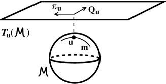
Figure 3.2: The two projectors $\pi^{\mu}_{\,\,\nu}$ and $Q^{\mu}_{\,\,\nu}$ split the tangent plane $T_{u}({\cal M})$ of a manifold ${\cal M}$ at the point $u$ into a direct sum of two orthogonal spaces $\pi_{u}$ and $Q_{u}$. Under certain circumstances (see the text for details), $\pi^{\mu}_{\,\,\nu}$ defines the tangent space of a submanifold m of ${\cal M}$.

It is worth emphasising that the only assumption we make from the outset is that the target space is a smooth manifold equipped with a (pseudo-) Riemannian metric and an antisymmetric two-tensor (the B-field). A priori we do not know anything about the properties of the D-brane; it need not be a regular submanifold of spacetime, and could be singular or ill-defined for all we know. Our object is to start from this unassuming standpoint and derive the properties required of the brane by superconformal invariance. It is thus by no means certain at this point that $\pi^{\mu}_{\,\,\nu}$ defines a tangent space corresponding to a submanifold of spacetime, although the vector space $\pi_{u}$ is a subspace of $T_{u}({\cal M})$. However, we will see in Section 3.7 that, under certain circumstances, this follows as a consequence of the superconformal boundary conditions.

We need one more object before writing down the boundary conditions. Given two orthogonal projectors $\pi^{\mu}_{\,\,\nu}$ and $Q^{\mu}_{\,\,\nu}$ we may define another (1,1)-tensor,

$$r^{\mu}_{\,\,\nu}\equiv\pi^{\mu}_{\,\,\nu}-Q^{\mu}_{\,\,\nu},$$

which squares to the identity, $r^{\mu}_{\,\,\nu}r^{\nu}_{\,\,\rho}=\delta^{\mu}_{\,\,\rho}$, since $\pi^{\mu}_{\,\,\nu}$ and $Q^{\mu}_{\,\,\nu}$ are orthogonal and each of them squares to itself. Alternatively, $\pi^{\mu}_{\,\,\nu}$ and $Q^{\mu}_{\,\,\nu}$ can be written in terms of $r^{\mu}_{\,\,\nu}$,

$$\pi^{\mu}_{\,\,\nu}=\frac{1}{2}\left(\delta^{\mu}_{\,\,\nu}+r^{\mu}_{\,\,\nu}\right),\quad\quad Q^{\mu}_{\,\,\nu}=\frac{1}{2}\left(\delta^{\mu}_{\,\,\nu}-r^{\mu}_{\,\,\nu}\right).$$

The three structures $\pi^{\mu}_{\,\,\nu}$, $Q^{\mu}_{\,\,\nu}$ and $r^{\mu}_{\,\,\nu}$, although very simple and intuitive in essence, were crucial in deriving and understanding the superconformal boundary conditions in Papers II and III. Note that initially they are defined only at a point, the endpoint of the string. However, we will see that superconformal invariance allows us to extend them to a neighbourhood, thus providing some information about the local smoothness of the brane. In fact, we will even define them globally (i.e. at every point in ${\cal M}$), just to see what happens. One can then draw some conclusions about the way in which the D-brane is embedded, globally, in spacetime, rather than merely looking at a small coordinate patch of the brane. But before exploring such possibilities, let us finally write down the boundary conditions explicitly.

3.6 The boundary conditions

Using the ansatz (3.7) and (3.8) in the current conditions (3.4) and (3.6), we found in Paper III the following three boundary conditions,

$$R^{\mu}_{\,\,\rho}G_{\mu\nu}R^{\nu}_{\,\,\sigma}=G_{\rho\sigma},$$ (3.14)

$$\pi^{\rho}_{\,\,\sigma}E_{\nu\rho}\pi^{\nu}_{\,\,\gamma}=\pi^{\rho}_{\,\,\sigma}E_{\rho\nu}\pi^{\nu}_{\,\,\lambda}R^{\lambda}_{\,\,\gamma},$$ (3.15)

$$\pi^{\rho}_{\,\,\sigma}\pi^{\nu}_{\,\,\lambda}\nabla_{[\rho}Q^{\mu}_{\,\,\nu]}=0.$$ (3.16)

We also showed that they make up a complete set, i.e. there are no further independent conditions to be found.

It may seem that these conditions are not in fact conditions on the worldsheet fields, which we claimed we were after. However, they are explicit conditions on the structures on the brane, which is equivalent to restrictions of the motion of the string endpoints.

The first condition says that the boundary map $R^{\mu}_{\,\,\nu}$ preserves the spacetime metric. This implies that the metric diagonalises so that it consists of a Neumann-Neumann part and a Dirichlet-Dirichlet part, but has no “mixed” components. One may see how this happens by going to adapted coordinates; there we have seen that $R^{\mu}_{\,\,\nu}$ has the diagonal form (3.12), so it follows immediately from (3.14) that the metric must be block-diagonal, $G_{\mu\nu}=\textstyle{\mathrm{diag}}(G_{mn},G_{ij})$.

There are two things to note here. First, the diagonal form of the metric does not necessarily imply that the two constituent blocks are completely decoupled. There may still be interdependence such that e.g. $G_{mn}$ depends on Dirichlet coordinates. Second, it is important to realise that the condition (3.14) is not imposing restrictions on the spacetime metric, but on the D-brane — its embedding in target space must be such that the metric diagonalises.

Moving on to the second boundary condition, Eq. (3.15), we see that it is a condition on the Neumann-Neumann part of $R^{\mu}_{\,\,\nu}$. It is essentially the definition of the B-field mentioned in Section 3.4; in adapted coordinates it schematically looks like $E^{-1}E^{T}=R$ (along the Neumann-Neumann directions). From this form we can derive the behaviour of the string for large B-field; as we take $B\rightarrow\infty$, the Neumann-Neumann block of $R^{\mu}_{\,\,\nu}$ goes to $-\delta^{m}_{\,\,n}$, i.e. we find that the Neumann conditions turn into Dirichlet conditions. That is, the endpoint of the string is completely frozen in all directions in this limit. It is also interesting to note that, in the limit $B\rightarrow 0$, we find $R^{\mu}_{\,\,\nu}\rightarrow r^{\mu}_{\,\,\nu}$.

Last but not least, we want to interpret the condition (3.16). This is actually a precise mathematical statement saying that the projector $\pi^{\mu}_{\,\,\nu}$ is integrable [51]. There are several ways of understanding the content of this statement [52], but perhaps the most intuitive one is to consider two displacements along the Neumann directions. If the commutator $[\delta_{1},\delta_{2}]X^{\mu}$ between them vanishes, then regardless of which order we do them in, we always end up in the same point. If, on the other hand, they do not commute, the final position will depend on the order of displacement. The latter case corresponds to some singular D-brane about which we cannot say much. The former situation, however, is the interesting one, because it occurs if and only if (3.16) holds, as is easily seen by inserting $\delta X^{\mu}=\pi^{\mu}_{\,\,\nu}\delta X^{\nu}$ in the commutator. It implies local smoothness at the point $u$ in the sense that we can extend the basis of $\pi_{u}$ to a neighbourhood of $u$ [53]. In particular the adapted coordinate basis, where $\pi^{\mu}_{\,\,\nu}$ takes the form

$$\pi^{\mu}_{\,\,\nu}=\left(\begin{array}[]{cc}\delta^{m}_{\,\,n}&0\\ 0&0\end{array}\right),$$ (3.17)

can be extended to a neighbourhood of $u$ so that $\pi^{\mu}_{\,\,\nu}$ is given by (3.17) on the whole neighbourhood. And since we can define $Q^{\mu}_{\,\,\nu}$ wherever $\pi^{\mu}_{\,\,\nu}$ is defined, and hence $r^{\mu}_{\,\,\nu}$, it follows that we may extend all three of our (1,1)-tensors to a neighbourhood of $u$.

Another consequence of $\pi$-integrability is that the Neumann-Neumann part of the metric is independent of the Dirichlet directions [52] (though as long as $Q^{\mu}_{\,\,\nu}$ is not integrable, the Dirichlet-Dirichlet part of $G_{\mu\nu}$ may still depend on the Neumann coordinates).

This is as far as we get in our interpretation of the conditions (3.14)–(3.16) without making additional assumptions. But the properties of our structures $Q^{\mu}_{\,\,\nu}$, $\pi^{\mu}_{\,\,\nu}$ and $r^{\mu}_{\,\,\nu}$ are exactly the same as those of the structures associated with almost product manifolds [52], except that they are not globally defined. We therefore found it irresistible to add this extra property in Papers II and III, and investigate the consequences.

3.7 Globally defined conditions

By “globally defined” we mean that our structures $Q^{\mu}_{\,\,\nu}$, $\pi^{\mu}_{\,\,\nu}$ and $r^{\mu}_{\,\,\nu}$, as well as $R^{\mu}_{\,\,\nu}$, all are defined not only at a point $u$ (and, by integrability, on a neighbourhood of $u$), but at every point $v$ in spacetime.

In this case, $\pi^{\mu}_{\,\,\nu}$ and $Q^{\mu}_{\,\,\nu}$ are distributions on ${\cal M}$ [51]. That is, they assign a space of vectors ($\pi_{v}$ and $Q_{v}$, respectively) to each point $v\in{\cal M}$, thus splitting the whole tangent space $T({\cal M})$ (not just the tangent plane at a point $u$, cf. Eq. (3.13)) into a direct sum,

$$T({\cal M})=\pi\oplus Q.$$ (3.18)

The tensor $r^{\mu}_{\,\,\nu}$ is now an almost product structure, defining the target space as an almost product manifold [52]. The word “almost” refers to the fact that the manifold is not necessarily a direct product, despite its tangent space being a direct sum. An example of such a manifold is a locally product manifold, i.e. a manifold that locally looks like a direct product but globally is not (think of the Möbius strip).

Let us have a fresh look at the boundary conditions (3.14)–(3.16) through our “global glasses.” We saw in Section 3.6 that the first condition implies that the metric diagonalises. In adapted coordinates it is then easily seen that the metric preserves also the almost product structure, since the latter takes the form

$$r^{\mu}_{\,\,\nu}=\left(\begin{array}[]{cc}\delta^{m}_{\,\,n}&0\\ 0&-\delta^{i}_{\,\,j}\end{array}\right)$$

in this basis. Thus the spacetime manifold is an almost product manifold with a (pseudo-) Riemannian metric that is preserved by the almost product structure; such a manifold is called a (pseudo-) Riemannian almost product manifold [52].

The second boundary condition, Eq. (3.15), gives no new information, so we turn directly to the condition (3.16), which says that $\pi^{\mu}_{\,\,\nu}$ is an integrable distribution. Such an object is by definition a foliation [53, 55]. This means that, at every point $v$ in spacetime, $\pi^{\mu}_{\,\,\nu}$ locally defines, on a neighbourhood of $v$, a set of hyperplanes, or leaves, that in adapted coordinates are described by the system of equations $\{X^{i}$= constant$\}$ [55]. These hyperplanes are contained in the space $\pi_{v}$, but a priori need not be of the same dimension, so they are not necessarily D-branes (recall that $\pi^{\mu}_{\,\,\nu}$ defines the dimensionality of the D-brane). However, there is a theorem by Frobenius saying that when $\pi^{\mu}_{\,\,\nu}$ is a foliation, then through every point $v\in{\cal M}$ there is a unique submanifold of ${\cal M}$ whose tangent space is $\pi_{v}$ (called a maximal integral manifold of $\pi^{\mu}_{\,\,\nu}$) [56]; this is the D-brane we were looking for.

In conclusion, globally defined superconformal boundary conditions imply that spacetime is foliated by D-branes which are submanifolds embedded in such a way that spacetime may be viewed as a (pseudo-) Riemannian almost product manifold. Let us give some concrete examples of such D-brane embeddings.

3.7.1 Examples

As we mentioned above, the obvious special case of an almost product manifold is a direct product, e.g. a torus (a direct product of one-cycles). Thus, if spacetime were a torus, the superconformally allowed D-branes would be those that wrap one or more of the constituent one-cycles.

More interestingly, many exact solutions of Einstein’s equations are almost product manifolds, e.g. the Schwarzschild and Robertson-Walker spaces. To be explicit, we take a closer look at the Schwarzschild space; it makes an instructive example of the way different D-brane embeddings determine the type of the spacetime manifold.

The Schwarzschild metric is

$$ds^{2}=-f(r)dt^{2}+h(r)dr^{2}+r^{2}d\Omega^{2},$$ (3.19)

where $t$ is time, $r$ is the radial coordinate, $f(r)\equiv 1-M/r$ with $M$ a constant, $h(r)\equiv 1/f(r)$, and $d\Omega^{2}$ is the metric on a two-sphere. Assuming that $t$ is the time coordinate also on the worldvolume of the D-brane, there is only one embedding which is allowed by the superconformal boundary conditions (3.14)–(3.16). We can write the manifold at hand as a warped product manifold

$$(\,{\cal M}_{1}\times{\cal M}_{2}\,,\,G_{1}(t,r)\oplus r^{2}G_{2}(\Omega^{2})\,),$$

with $G_{1}(t,r)\equiv-f(r)dt^{2}+h(r)dr^{2}$ being the metric on ${\cal M}_{1}$ and $G_{2}(\Omega^{2})\equiv d\Omega^{2}$ the metric on ${\cal M}_{2}$. It is called “warped” because the factor in front of $G_{2}$ (in our case $r^{2}$) depends on the coordinates of ${\cal M}_{1}$. Then the brane can extend along $t$ and $r$, i.e. we have a D1-brane that coincides with the manifold ${\cal M}_{1}$. Here $G_{1}(t,r)$ is the metric on the brane; it is independent of the ${\cal M}_{2}$-coordinates, which is consistent with integrability of $\pi^{\mu}_{\,\,\nu}$. On the other hand, there is a problem with integrability at the singularity $r=0$; nevertheless, the general principle should be clear.

Alternatively, we may write the metric (3.19) as a different almost product manifold,

$$(\,{\cal M}_{1}\times{\cal M}_{2}\,,\,G_{1}(t,r,\Omega^{2})\oplus G_{2}(r)\,),$$

with $G_{1}(t,r,\Omega^{2})\equiv-f(r)dt^{2}+r^{2}d\Omega^{2}$ and $G_{2}(r)\equiv h(r)dr^{2}$. Here we could have a D2-brane wrapping ${\cal M}_{1}$. However, it would not be superconformal, since $\pi^{\mu}_{\,\,\nu}$ is not integrable in this case; the Neumann-Neumann metric $G_{1}(t,r,\Omega^{2})$ depends on the Dirichlet direction $r$. Finally, there is also the possibility of a D0-brane, extending only along $t$, in which case spacetime again is a warped product manifold, with warp factor $-f(r)$. Also this brane breaks superconformal invariance, since the metric on the brane depends on the Dirichlet directions.

The various embeddings are illustrated in Fig. 3.3.

Figure 3.3: Various D-brane embeddings in a Schwarzschild space. The Schwarzschild space is represented here by a two-sphere, and the D-branes are, respectively, a D2-brane wrapping the two-sphere part of the Schwarzschild space (represented here by a circle), a D1-brane extending along the radius, and a D0-brane, which is just a point in the spacelike directions. Only the D1-brane is allowed by the globally defined superconformal boundary conditions (3.14)–(3.16).

3.8 The WZW model

In the preceding sections we have learnt the minimal requirements for a D-brane to preserve superconformal symmetry in a general spacetime. To put our boundary conditions to the test, we want to study a special case, i.e. a string propagating on a given manifold. The most obvious choice is the extensively studied WZW model [44]. This is a nonlinear sigma model defined on a group manifold of some Lie group $G$; that is, the target space coordinates transform into each other under a group $G$. The importance of this model is due to the fact that it is exactly solvable, and provides a tractable setting for studying D-branes in curved backgrounds. In particular, when $G$ is a semisimple Lie group, the background fields simplify in such a way as to make our boundary conditions more transparent.

3.8.1 Symmetries

The target space (and the action) is invariant under $G\times G$ transformations, so there are two chiral currents (i.e. each current depends only on one of the worldsheet coordinates $\xi^{\pm}$) associated with this symmetry, one for each group $G$. They can be derived from the superspace action (3.5) by varying it with respect to the “left” and “right” group, respectively. The result is left- and right-moving currents,

$$J_{+}\equiv-\mathbf{l}_{\,\,\mu}D_{+}\Phi^{\mu},\quad\quad J_{-}\equiv\mathbf{r}_{\,\,\mu}D_{-}\Phi^{\mu},$$

where $\mathbf{l}_{\,\,\mu}$ and $\mathbf{r}_{\,\,\mu}$ are the superfield Killing vectors associated with each symmetry. We denote the lowest (fermionic) components of $J_{\pm}$ by

$$j_{+}\equiv J_{+}|=-l_{\mu}\psi_{+}^{\mu},\quad\quad j_{-}\equiv J_{-}|=r_{\mu}\psi_{-}^{\mu},$$ (3.20)

where $l_{\mu}$ and $r_{\mu}$ are the lowest components of the superfield Killing vectors.

The vectors $l^{\mu}$ and $r^{\mu}$ can be expanded in the Lie algebra basis $\{T^{A}\}$ of their corresponding groups, as $l^{\mu}\equiv l^{\mu}_{\,\,A}T^{A}$ and $r^{\mu}\equiv r^{\mu}_{\,\,A}T^{A}$. Then the coefficients $l^{\mu}_{\,\,A}$ and $r^{\mu}_{\,\,A}$ satisfy the corresponding Lie algebra,

$$[l_{A},l_{B}]=-f_{AB}^{\,\,\,\,\,\,\,\,\,C}l_{C},\quad\quad[r_{A},r_{B}]=f_{AB}^{\,\,\,\,\,\,\,\,\,C}r_{C}$$

(the sign is just a convention), and they commute with each other, $[l_{A},r_{B}]=0$. Here the Lie bracket for vectors $v^{\mu}_{\,\,A}$ is defined as $[v_{A},v_{B}]^{\mu}\equiv v^{\nu}_{\,\,A}\partial_{\nu}v^{\mu}_{\,\,B}-v^{\nu}_{\,\,B}\partial_{\nu}v^{\mu}_{\,\,A}$.

3.8.2 The gluing map

From (3.20) follows immediately that the fermionic ansatz (3.7) translates into a boundary condition for the group currents,

$$j^{A}_{-}=\eta\,R^{A}_{\,\,\,B}\,j^{B}_{+},$$

where

$$R^{A}_{\,\,\,B}\equiv-l^{A}_{\,\,\mu}R^{\mu}_{\,\,\,\nu}r^{\nu}_{\,\,B}.$$ (3.21)

The transformation in (3.21) is essentially a change of basis from spacetime vectors to the Lie algebra basis [45].

The object $R^{A}_{\,\,\,B}$ is a gluing map between the chiral currents at the worldsheet boundary. Since it maps $j^{B}_{+}$ to $j^{A}_{-}$, which are elements of the Lie algebra, it is clearly a map from the Lie algebra into itself. What more we can say about this map? It is usually assumed in the literature to be a constant Lie algebra automorphism [45, 57, 58]. This means that it preserves the Lie algebra structure in the sense that

$$\left[R^{C}_{\,\,\,A}T_{C},R^{D}_{\,\,\,B}T_{D}\right]=f_{AB}^{\,\,\,\,\,\,\,\,\,C}R^{F}_{\,\,\,C}T_{F}.$$ (3.22)

However, this restriction is always made for practical reasons, as a nonconstant gluing map makes the quantum theory unwieldy. And indeed we found in Paper IV that $R^{A}_{\,\,\,B}$ in the ${\cal N}$=1 model can in principle be a much more general object.

To see how we reach this conclusion, let us write down the boundary conditions for the WZW model. For this purpose, we take advantage of the fact that on group manifolds the metric and torsion can be expressed entirely in terms of Killing vectors, Lie algebra structure constants and the Cartan-Killing metric $\eta_{AB}$ [59]. As a consequence, the boundary conditions (3.14) and (3.16) can be written as equations involving only these quantities plus $R^{A}_{\,\,\,B}$, and we end up with the following conditions,

$$\eta_{AB}=R^{C}_{\,\,\,A}\eta_{CD}R^{D}_{\,\,\,B},$$ (3.23)

$$f_{ABC}-f_{DEF}R^{D}_{\,\,\,A}R^{E}_{\,\,\,B}R^{F}_{\,\,\,C}=\eta_{DE}R^{D}_{\,\,\,[A}\left({\cal L}_{C}R^{E}_{\,\,\,B]}\right).$$ (3.24)

Here the Lie derivative is defined as

$${\cal L}_{C}R^{E}_{\,\,\,B}\equiv{\cal L}_{r_{C}}R^{E}_{\,\,\,B}-R^{H}_{\,\,\,C}{\cal L}_{l_{H}}R^{E}_{\,\,\,B}=\left(r^{\mu}_{C}-R^{H}_{\,\,\,C}l^{\mu}_{H}\right)R^{E}_{\,\,\,B,\mu},$$

with ${\cal L}_{r_{C}}$ the usual Lie derivative with respect to the vector $r^{\mu}_{\,\,C}$.

The first condition, Eq. (3.23), says that the gluing map preserves the Cartan-Killing metric. But it is the second condition, Eq. (3.24), that interests us. To see what it means, let us first use (3.23) to manipulate the Lie bracket (3.22) a little. We can rewrite the left-hand side of (3.22) as

$$R^{D}_{\,\,\,A}R^{E}_{\,\,\,B}\left[T_{D},T_{E}\right]=R^{D}_{\,\,\,A}R^{E}_{\,\,\,B}f_{DE}^{\,\,\,\,\,\,\,\,\,F}T_{F},$$

whence, using (3.23), follows that $R^{A}_{\,\,\,B}$ is a Lie algebra automorphism if and only if

$$f_{ABC}-f_{DEF}R^{D}_{\,\,\,A}R^{E}_{\,\,\,B}R^{F}_{\,\,\,C}=0.$$

Thus we see that $R^{A}_{\,\,\,B}$ is a Lie algebra automorphism if and only if the right-hand side of (3.24) vanishes.

Hence we draw two conclusions from (3.24). First, $R^{A}_{\,\,\,B}$ does not have to be a Lie algebra automorphism. Second, it can be a Lie algebra automorphism without being constant, since the right-hand side can vanish even if $R^{A}_{\,\,\,B}$ is nonconstant. The interpretation of this condition in terms of D-branes was not addressed in Paper IV, but it is known that for the special case where $R^{A}_{\,\,\,B}$ is constant, conformally invariant D-branes are obtained as conjugacy classes of the group $G$ [57].

Bibliography

- [1] A. Bilal, Higher-derivative corrections to the non-abelian Born-Infeld action, Nucl. Phys. B618 (2001) 21-49, hep-th/0106062.
- [2] P. Koerber and A. Sevrin, The non-abelian D-brane effective action through order , JHEP 0210 (2002) 046, hep-th/0208044.
- [3] B. R. Greene, String Theory on Calabi-Yau Manifolds, TASI lecture notes (1996), hep-th/9702155.
- [4] P. S. Aspinwall, K3 surfaces and string duality, TASI lecture notes (1996), hep-th/9611137.
- [5] J. Polchinski, String theory, Vol II (Cambridge University Press, 1998).
- [6] K. Intriligator and N. Seiberg, Mirror Symmetry in Three Dimensional Gauge Theories, Phys. Lett. B387 (1996) 513-519, hep-th/9607207.
- [7] P. B. Kronheimer, The construction of ALE spaces as Hyper-Kähler quotients, J. Diff. Geom. 29 (1989) 665.
- [8] U. Lindström, M. Roček and R. von Unge, Hyperkähler quotients and algebraic curves JHEP 0001 (2000) 022, hep-th/9908082.
- [9] I. Y. Park and R. von Unge, Hyperkähler quotients, mirror symmetry, and F-theory, JHEP 0003 (2000) 037, hep-th/0001051.
- [10] W. Fulton and J. Harris, Representation Theory: A First Course (Springer-Verlag, 1991).
- [11] L. H. Ryder, Quantum field theory (Cambridge University Press, 1996).
- [12] M. Maggiore, Champs et Particules, Chapter 9, lecture notes 2001/02, Département de Physique Théorique de l’Université de Genéve.
- [13] A. Bilal, Duality in =2 susy Yang-Mills theory: A pedagogical introduction to the work of Seiberg and Witten, hep-th/9601007.
- [14] C. V. Johnson and R. C. Myers, Aspects of Type IIB theory on ALE spaces, Phys. Rev. D55 (1997) 6382-6393, hep-th/9610140.
- [15] J. Wess and J. Bagger, Supersymmetry and supergravity (Princeton University Press, 1992).
- [16] P. S. Aspinwall, Compactification, geometry and duality: N=2, TASI lecture notes (1999), hep-th/0001001.
- [17] N. J. Hitchin, A. Karlhede, U. Lindström and M. Roček, Hyperkähler metrics and supersymmetry, Commun. Math. Phys. 108 (1987) 535-589.
- [18] W. Lerche, Introduction to Seiberg-Witten theory and its stringy origin, Nucl. Phys. Proc. Suppl. 55B (1997) 83-117; Fortsch. Phys. 45 (1997) 293-340, hep-th/9611190.
- [19] N. Seiberg and E. Witten, Monopole condensation and confinement in N=2 supersymmetric Yang-Mills theory, Nucl. Phys. B426 (1994) 19-52; Erratum-ibid. B430 (1994) 485-486, hep-th/9407087.
- [20] P. C. Argyres, M. R. Plesser and N. Seiberg, The moduli space of N=2 SUSY QCD and duality in N=1 SUSY QCD, Nucl. Phys. B471 (1996) 159-194, hep-th/9603042.
- [21] N. Koblitz, Introduction to elliptic curves and modular forms, 2nd ed. (Springer-Verlag, 1993).
- [22] K. Kodaira, On compact analytic surfaces, II-III, Ann. of Math. 77 (1963) 563; 78 (1963) 1.
- [23] P. C. Argyres, M. R. Plesser, N. Seiberg and E. Witten, New N=2 superconformal field theories in four dimensions, Nucl. Phys. B461 (1996) 71, hep-th/9511154.
- [24] T. Eguchi, K. Hori, K. Ito and S.-K. Yang, Study of N=2 superconformal field theories in 4 dimensions, Nucl. Phys. B471 (1996) 430, hep-th/9603002.
- [25] J. Minahan and D. Nemeschansky, An N=2 superconformal fixed points with global symmetry, Nucl. Phys. B482 (1996) 142-152, hep-th/9608047.
- [26] J. Minahan and D. Nemeschansky, Superconformal fixed points with global symmetry, Nucl. Phys. B489 (1997) 24-46, hep-th/9610076.
- [27] M. Noguchi, S. Terashima and S.-K. Yang, N=2 superconformal field theory with ADE global symmetry on a D3-brane probe, Nucl. Phys. B556 (1999) 115-151, hep-th/9903215.
- [28] N. Seiberg, Five dimensional SUSY field theories, non-trivial fixed points and string dynamics, Phys. Lett. B388 (1996) 753-760, hep-th/9608111.
- [29] W. Lerche and N. P. Warner, Exceptional SW geometry from ALE fibrations, Phys. Lett. B423 (1998) 79-86, hep-th/9608183.
- [30] C. Vafa, Evidence for F-Theory, Nucl. Phys. B469 (1996) 403-418, hep-th/9602022.
- [31] A. Johansen, A comment on BPS states in F-theory in 8 dimensions, Phys. Lett. B395 (1997) 36, hep-th/9608186.
- [32] M. R. Gaberdiel and B. Zwiebach, Exceptional groups from open strings, Nucl. Phys. B518 (1998) 151-172, hep-th/9709013.
- [33] T. Banks, M. Douglas and N. Seiberg, Probing F-theory with branes, Phys. Lett. B387 (1996) 278, hep-th/9605199.
- [34] A. Fayyazuddin and M. Spalinski, The Seiberg-Witten differential from M-Theory, Nucl. Phys. B508 (1997) 219-228, hep-th/9706087.
- [35] O. Aharony, A. Fayyazuddin and J. Maldacena, The large N limit of field theories from threebranes in F-theory, JHEP 9807 (1998) 013, hep-th/9806159.
- [36] A. Sen, F-theory and orientifolds, Nucl. Phys. B475 (1996) 562-578, hep-th/9605150.
- [37] B. Feng, A. Hanany, Y.-H. He and N. Prezas, Stepwise projection: toward brane setups for generic orbifold singularities, JHEP 0201 (2002) 040, hep-th/0012078.
- [38] M. Douglas and G. Moore, D-branes, quivers, and ALE instantons, hep-th/9603167.
- [39] J. Polchinski, String theory, Vol I (Cambridge University Press, 1998).
- [40] D. Mumford and J. Fogarty, Geometric invariant theory (Springer, 1982).
- [41] C. Albertsson, B. Brinne, U. Lindström, M. Roček and R. von Unge, ADE-quiver theories and mirror symmetry, Nucl. Phys. B Proc. Suppl. 102 & 103 (2001) 3-10, hep-th/0103084.
- [42] U. Lindström and M. Zabzine, N=2 boundary conditions for non-linear sigma models and Landau-Ginzburg models, JHEP 0302 (2003) 006, hep-th/0209098.
- [43] U. Lindström and M. Zabzine, D-branes in N=2 WZW models, to appear in Phys. Lett. B, hep-th/0212042.
- [44] K. Gawedzki, Conformal field theory: a case study, hep-th/9904145.
- [45] S. Stanciu, D-branes in group manifolds, JHEP 0001 (2000) 025, hep-th/9909163.
- [46] M. B. Green, J. H. Schwarz and E. Witten, Superstring theory, Vol I (Cambridge University Press, 1987).
- [47] M. B. Green, J. H. Schwarz and E. Witten, Superstring theory, Vol II (Cambridge University Press, 1987).
- [48] F. Bastianelli and U. Lindström, Induced chiral supergravities in 2D, Nucl. Phys. B416 (1994) 227, hep-th/9303109.
- [49] H. Ooguri, Y. Oz and Z. Yin, D-branes on Calabi-Yau spaces and their mirrors, Nucl. Phys. B477 (1996) 407-430, hep-th/9606112.
- [50] E. Alvarez, J. L. F. Barbon and J. Borlaf, T-duality for open strings, Nucl. Phys. B479 (1996) 218-242, hep-th/9603089.
- [51] K. Yano, Differential geometry on complex and almost complex spaces (Pergamon, Oxford, 1965).
- [52] K. Yano and M. Kon, Structures on manifolds, Series in Pure Mathematics, Vol 3 (World Scientific, Singapore, 1984).
- [53] B. L. Reinhart, Differential geometry of foliations (Springer-Verlag, 1983).
- [54] A. Borowiec, M. Ferraris, M. Francaviglia and I. Volovich, Almost complex and almost product Einstein manifolds from a variational principle, J. Math. Phys. 40 (1999) 3446-3464, dg-ga/9612009.
- [55] P. Tondeur, Foliations on Riemannian manifolds (Springer-Verlag, New York, 1988).
- [56] W. M. Boothby, An introduction to differentiable manifolds and Riemannian geometry (Academic Press, London, 1986).
- [57] A. Y. Alekseev and V. Schomerus, D-branes in the WZW model, Phys. Rev. D60 (1999) 061901, hep-th/9812193.
- [58] T. Itoh and S.-J. Sin, A note on singular D-branes in group manifolds, Nucl. Phys. B650 (2003) 497-521, hep-th/0206238.
- [59] C. M. Hull and B. Spence, The gauged nonlinear sigma model with Wess-Zumino term, Phys. Lett. B232 (1989) 204.