^a Theory Division
CERN
CH-1211 Geneva 23
Switzerland
 
^b Institute of Theoretical Physics
University of Bern
CH-3012 Bern
Switzerland
 

We investigate $B$-type topological Landau-Ginzburg theory with one variable, with $D2$-brane boundary conditions. The allowed brane configurations are determined in terms of the possible factorizations of the superpotential, and compute the corresponding open string chiral rings. These are characterized by bosonic and fermionic generators that satisfy certain relations. Moreover we show that the disk correlators, being continuous functions of deformation parameters, satisfy the topological sewing constraints, thereby proving consistency of the theory. In addition we show that the open string LG model is, in its content, equivalent to a certain triangulated category introduced by Kontsevich, and thus may be viewed as a concrete physical realization of it.

Landau-Ginzburg Realization of Open String TFT

1 Introduction and Summary

The understanding of open-closed topological field theory (TFT) in two dimensions is an important issue in string theory, for it represents a framework to describe the vacuum structure of space-time in the presence of $D$-branes. The works [1, 2, 3] provide us with an axiomatic definition of open-closed TFT via sewing constraints on Riemann surfaces with boundaries, which can be given a formulation in terms of non-commutative Frobenius algebras [4]. In a somewhat different spirit, namely by focusing on cohomological aspects, 2d open string TFT has been investigated for example in [5, 6] and in [7, 8]. A further, though closely related point of view is based on derived categories, which is the general mathematical framework that underlies $D$-branes [9, 10]; aspects of open string TFT from this perspective have been discussed, for example, in [11, 12, 13, 14, 15, 16, 17, 7, 18].

In order to get a better understanding of the interrelation between these more abstract viewpoints, it is desirable to investigate concrete physical realizations of such open-closed TFT’s. First steps were made by formulating boundary linear sigma models [19, 20, 21, 22, 23, 24, 25, 26]; these provide a framework to represent quite general $D$-brane configurations, mathematically defined in terms of bundles and sheaves localized on sub-manifolds, in terms of physical operators.

On the other hand, one can study boundary Landau-Ginzburg models with superpotentials depending on continuous parameters, with the expectation to be able to perform functionally non-trivial explicit computations. This is partly motivated from the experience with the topologically twisted LG theories in the bulk, for which it is often possible to determine the correlation functions by just using consistency conditions [27, 28, 29]. Such Landau-Ginzburg models, apart from being very concrete, also often allow to make direct contact with an exactly solvable CFT description of a given theory. Moreover, they provide a natural setting for the application of mirror symmetry [7].

So far, most approaches to a Landau-Ginzburg realization of $B$-type, open-closed TFT’s have focused on Dirichlet boundary conditions for the fields, which correspond to $D0$-branes [19, 20, 22, 2, 7]. In the present paper we extend this line of research by working out in detail the “minimal” topological LG model with one variable, however with $D2$-brane boundary conditions which turn out to provide a much richer structure. Some general aspects of this model, as well as a detailed analysis for quadratic superpotentials, have been presented recently in [30].

Specifically, we will confirm that the possible supersymmetric $D2$-brane configurations correspond to the different possible factorizations of the bulk superpotential. For each such brane configuration, as well as for each pair of such configurations, we will work out the topological open string spectrum, i.e., the boundary chiral ring. As an important feature, this ring contains bosonic as well as a fermionic generators, both of which satisfy certain relations determined by the factorization data of the superpotential.

We will verify that in the unperturbed limit, the spectra match exactly with the corresponding chiral ring elements known from the BCFT description of B-type branes [31, 32, 33]. In the perturbed theory, the spectrum of boundary changing operators depends critically on the divisibility properties of certain polynomials, and we observe an intriguing branching of the spectrum for generic perturbations.

We will also determine a specific basis for the boundary preserving operators, which allows to write down in an easy way all disk correlation functions in the boundary preserving open string sectors. Next we will demonstrate that the topological sewing constraints that we mentioned above, are indeed satisfied by these disk correlators. The proof applies to whole families of continuously deformed LG theories, and involves the factorization of the superpotential and the fermionic ring relations in a crucial manner (this goes far beyond the usual analysis of sewing constraints which is based on rational BCFT and which therefore applies only to a given, fixed theory).

Moreover we will make contact with a formulation of $B$-type $D$-branes in terms of certain triangulated categories, which is due to Kontsevich. Extending the work of [30, 34], we will in particular show that the underlying cohomology problems are isomorphic, and thus lead to the same open string spectrum. From this point of view, the boundary LG formulation provides a concrete physical realization of this abstract mathematical framework.

We thus have good reasons to expect that extending our work to more general theories will provide further insights in the relationship between open-closed TFT and the categorial descriptions of $D$-branes, apart from sharpening our technical tools for doing explicit computations.

Acknowledgment: We thank Albert Schwarz for discussions.

2 $B$-type boundary conditions in LG models

Starting with the familiar 2-dimensional $(2,2)$-supersymmetric Landau-Ginzburg model for the bulk, one can study the effects of introducing a world sheet boundary [35, 19, 20, 22, 21, 30]. As is well known, the boundary breaks one half of the supersymmetries and there essentially remain two types of symmetries [35], which correspond to $A$- and $B$-type $D$-branes [36]. In the present paper we will restrict ourselves to unbroken $B$-type supersymmetry and include a boundary action such that the total action is invariant under supersymmetry variations without imposing any particular boundary conditions. This approach was used in [35], where it turned out that in order to achieve this, one has to introduce a fermionic supermultiplet on the boundary. We will see in the next section that the boundary fermion plays an essential role in the construction of the open string chiral ring.

The main purpose of the present section is to define the physical setting described above and to fix the notation.

2.1 Bulk action

The $(2,2)$-superspace in two dimensions is spanned by two bosonic coordinates $(x^{0},x^{1})$ and four fermionic coordinates $\theta^{\pm},\bar{\theta}^{\pm}$ (with $(\theta^{\pm})^{\dagger}=\bar{\theta}^{\pm}$). The supercharges and covariant derivatives are represented by

$$Q_{\pm}=\frac{\partial}{\partial\theta^{\pm}}+i\bar{\theta}^{\pm}\frac{\partial}{\partial x^{\pm}}\>,\qquad\bar{Q}_{\pm}=-\frac{\partial}{\partial\bar{\theta}^{\pm}}-i\theta^{\pm}\frac{\partial}{\partial x^{\pm}}\>,$$ (1)

and

$$D_{\pm}=\frac{\partial}{\partial\theta^{\pm}}-i\bar{\theta}^{\pm}\frac{\partial}{\partial x^{\pm}}\>,\qquad\bar{D}_{\pm}=-\frac{\partial}{\partial\bar{\theta}^{\pm}}+i\theta^{\pm}\frac{\partial}{\partial x^{\pm}}\>,$$ (2)

where $x^{\pm}=x^{0}\!\pm\!x^{1}$. They satisfy the supersymmetry algebra

$$\{Q_{\pm},\bar{Q}_{\pm}\}=-2i\partial_{\pm}\>,\quad\{D_{\pm},\bar{D}_{\pm}\}=2i\partial_{\pm}\>.$$ (3)

In the Landau-Ginzburg theory we introduce a chiral and an antichiral superfield $\Phi$ and $\bar{\Phi}$, i.e., $\bar{D}_{\pm}\Phi=0$ and $D_{\pm}\bar{\Phi}=0$. The expansion in component fields reads

$$\Phi(y^{\pm},\theta^{\pm})=\phi(y^{\pm})+\theta^{+}\psi_{+}(y^{\pm})+\theta^{-}\psi_{-}(y^{\pm})+\theta^{+}\theta^{-}F(y^{\pm})\;,$$

where $y^{\pm}=x^{\pm}\!\!-\!i\theta^{\pm}\bar{\theta}^{\pm}$. If we set $\delta=\epsilon_{+}Q_{-}-\epsilon_{-}Q_{+}-\bar{\epsilon}_{+}\bar{Q}_{-}+\bar{\epsilon}_{-}\bar{Q}_{+}$, the variations of the fields take the form

$$\begin{array}[]{cc}\begin{array}[]{l@{\;=\;}l}\delta\phi&+\epsilon_{+}\psi_{-}-\epsilon_{-}\psi_{+}\;,\\[2.84526pt] \delta\psi_{+}&+2i\bar{\epsilon}_{-}\partial_{+}\phi+\epsilon_{+}F\;,\\[2.84526pt] \delta\psi_{-}&-2i\bar{\epsilon}_{+}\partial_{-}\phi+\epsilon_{-}F\;,\end{array}&\begin{array}[]{l@{\;=\;}l}\delta\bar{\phi}&-\bar{\epsilon}_{+}\bar{\psi}_{-}+\bar{\epsilon}_{-}\bar{\psi}_{+}\;,\\[2.84526pt] \delta\bar{\psi}_{+}&-2i\epsilon_{-}\partial_{+}\bar{\phi}+\bar{\epsilon}_{+}\bar{F}\;,\\[2.84526pt] \delta\bar{\psi}_{-}&+2i\epsilon_{+}\partial_{-}\bar{\phi}+\bar{\epsilon}_{-}\bar{F}\;.\end{array}\end{array}$$ (11)

In terms of the chiral and antichiral superfields one can build two supersymmetric contributions for the action. The $D$-term is an integral of a function $K(\Phi,\bar{\Phi})$ over the full superspace. Since we are interested only in topological quantities which do not depend on the $D$-term, we choose $K(\Phi,\bar{\Phi})=\bar{\Phi}\Phi$ for simplicity. The second part is the $F$-term,

$$\int_{{\Sigma}}d^{2}xd^{2}\theta\,W(\Phi)\bigr{|}_{\bar{\theta}^{\pm}=0}+\textrm{c.c.}\;.$$ (12)

It contains the world sheet superpotential, which fully determines the topological sector of the bulk theory. Up to total derivatives, the bulk action can be written as

$$\begin{array}[]{ccc}S_{\Sigma}&=&\displaystyle{\int_{{\Sigma}}d^{2}x\left\{-\partial^{\mu}\bar{\phi}\partial_{\mu}\phi+\frac{i}{2}\bar{\psi}_{-}(\stackrel{{\scriptstyle\leftrightarrow}}{{\partial_{0}}}+\stackrel{{\scriptstyle\leftrightarrow}}{{\partial_{1}}})\psi_{-}+\frac{i}{2}\bar{\psi}_{+}(\stackrel{{\scriptstyle\leftrightarrow}}{{\partial_{0}}}-\stackrel{{\scriptstyle\leftrightarrow}}{{\partial_{1}}})\psi_{+}\right.}\\ &&\left.\displaystyle{-\frac{1}{4}|W^{\prime}|^{2}-\frac{1}{2}W^{\prime\prime}\psi_{+}\psi_{-}-\frac{1}{2}\bar{W}^{\prime\prime}\bar{\psi}_{-}\bar{\psi}_{+}}\right\}\>,\end{array}$$ (13)

where the algebraic equation of motion $F=-1/2\,\bar{W}^{\prime}(\bar{\phi})$ was used.

2.2 Introduction of boundary degrees of freedom

If we wish to formulate our theory on a world sheet with boundary, one recognizes first that the translation symmetry normal to the boundary is broken and, therefore, also one-half of the supersymmetries are broken [35, 36]. We choose the world sheet $\Sigma$ to be given by the strip with coordinates $(x^{0},x^{1})\in(\mathbb{R},[0,\pi])$. We are interested in $B$-type supersymmetry with preserved supercharge $Q=\bar{Q}_{+}+(-1)^{S}\bar{Q}_{-}$. In terms of the parameters $\epsilon_{\pm}$ one can describe $B$-type supersymmetry by setting $\epsilon=\epsilon_{+}=(-1)^{S+1}\epsilon_{-}$. For convenience we set $S=0$ and put the fermions together into the combinations $\eta=\psi_{-}\!\!+\!\psi_{+}$ and $\theta=\psi_{-}\!\!-\!\psi_{+}$. Therefore, the $B$-type supersymmetry transformations ($\delta=\epsilon\bar{Q}-\bar{\epsilon}Q$) read

$$\begin{array}[]{cc}\begin{array}[]{l@{\;=\;}l}\delta\phi&\epsilon\eta\;,\\[2.84526pt] \delta\eta&-2i\bar{\epsilon}\partial_{0}\phi\;,\\[2.84526pt] \delta\theta&2i\bar{\epsilon}\partial_{1}\phi+\epsilon\bar{W}^{\prime}(\bar{\phi})\;,\end{array}&\begin{array}[]{l@{\;=\;}l}\delta\bar{\phi}&-\bar{\epsilon}\bar{\eta}\;,\\[2.84526pt] \delta\bar{\eta}&2i\epsilon\partial_{0}\bar{\phi}\;,\\[2.84526pt] \delta\bar{\theta}&-2i\epsilon\partial_{1}\bar{\phi}+\bar{\epsilon}W^{\prime}(\phi)\;.\end{array}\end{array}$$ (14)

The boundary superspace is spanned by the coordinates $\theta^{0}=1/2(\theta^{-}\!\!+\!\theta^{+})$ and $\bar{\theta}^{0}=1/2(\bar{\theta}^{-}\!\!+\!\bar{\theta}^{+})$, so that the supercharges become

$$\bar{Q}=\frac{\partial}{\partial\theta^{0}}+i\bar{\theta}^{0}\frac{\partial}{\partial x^{0}}\qquad\textrm{and}\qquad Q=-\frac{\partial}{\partial\bar{\theta}^{0}}-i\theta^{0}\frac{\partial}{\partial x^{0}}\;.$$ (15)

From equations (14) we see that the fields of the chiral multiplet $\Phi$ in the bulk rearrange into a bosonic and a fermionic multiplet $\Phi^{\prime}$ and $\Theta^{\prime}$, respectively. The bosonic superfield $\Phi^{\prime}$ containing $\phi$ and $\eta$ turns out to be chiral, i.e., $D\,\Phi^{\prime}=0$, whereas the variation of $\Theta^{\prime}$ contains the term $\partial_{1}\phi$, which cannot be accomplished by (15). This means that $\theta$ and $F$ do not form a chiral multiplet, but rather combine into the fermionic superfield $\Theta^{\prime}$ which satisfies $D\,\Theta^{\prime}=-2i\partial_{1}\Phi^{\prime}$. In components we have

$$\Phi^{\prime}(y^{0},\theta^{0}) = \phi(y^{0})+\theta^{0}\eta(y^{0}),$$

$$\Theta^{\prime}(y^{0},\theta^{0},\bar{\theta}^{0}) = \theta(y^{0})-2\theta^{0}F(y^{0})+2i\;\bar{\theta}^{0}\bigl{[}\partial_{1}\phi(y^{0})+\theta^{0}\partial_{1}\eta(y^{0})\bigr{]},$$ (16)

where $y^{0}=x^{0}-i\theta^{0}\bar{\theta}^{0}$.

Now we turn back to the Lagrangian and construct the necessary boundary terms in order to get a fully supersymmetric action. If we set $W=0$, the $B$-type supersymmetry variation of the bulk action (13) gives rise to a surface term that can be compensated by

$$S_{{\partial{\Sigma}},\psi}=\frac{i}{4}\int\!dx^{0}\,\left\{\bar{\theta}\eta-\bar{\eta}\theta\right\}\Bigr{|}_{0}^{\pi}\>.$$ (17)

If we turn on the superpotential $W$ the following surface term:

$$\delta(S_{\Sigma}+S_{{\partial{\Sigma}},\psi})=\frac{i}{2}\int\!dx^{0}\,\left\{\epsilon\bar{\eta}\bar{W}^{\prime}+\bar{\epsilon}\eta W^{\prime}\right\}\Bigr{|}_{0}^{\pi}\>$$ (18)

remains from the variation. It cannot be compensated by any boundary action containing bulk fields, because the combination $\epsilon\bar{\eta}$ occurs, whereas the transformations (14) generate only $\epsilon\eta$.

In order to ensure invariance of the action we need to introduce an additional superfield on the boundary which is capable to compensate (18). Following [35] we introduce a boundary fermionic superfield $\Pi$, which is not chiral but rather satisfies: $D\,\Pi=E(\Phi^{\prime})$, and which has the expansion

$$\Pi(y^{0},\theta^{0},\bar{\theta}^{0})=\pi(y^{0})+\theta^{0}\,l(y^{0})-\bar{\theta}^{0}\,\bigl{[}E(\phi)+\theta^{0}\eta(y^{0})E^{\prime}(\phi)\bigr{]}\;.$$ (19)

Its component fields transform as:

$$\begin{array}[]{cc}\begin{array}[]{l@{\;=\;}l}\delta\pi&\epsilon l-\bar{\epsilon}E(\phi)\;,\\[2.84526pt] \delta l&-2i\bar{\epsilon}\partial_{0}\pi+\bar{\epsilon}\eta E^{\prime}(\phi),\end{array}&\begin{array}[]{l@{\;=\;}l}\delta\bar{\pi}&\bar{\epsilon}\bar{l}-\epsilon\bar{E}(\bar{\phi})\;,\\[2.84526pt] \delta\bar{l}&-2i\epsilon\partial_{0}\bar{\pi}-\epsilon\bar{\eta}\bar{E}^{\prime}(\bar{\phi})\;.\end{array}\end{array}$$ (20)

Similar to the bulk theory we can build two terms for the action, i.e.,

$$S_{\partial{\Sigma}}=-\frac{1}{2}\int\!\!dx^{0}d^{2}\theta\,\bar{\Pi}\;\Pi\Bigr{|}_{0}^{\pi}\,-\frac{i}{2}\int_{\partial{\Sigma}}\!\!dx^{0}d\theta\,\Pi\;J(\Phi)\,_{\bar{\theta}=0}\Bigr{|}_{0}^{\pi}+\textrm{c.c.}\;.$$ (21)

Using the algebraic equation of motion $l=-i\bar{J}(\bar{\phi})$, the boundary action reads

$$S_{\partial{\Sigma}}=\int\!dx^{0}\left\{i\bar{\pi}\partial_{0}\pi-\frac{1}{2}\bar{J}J-\frac{1}{2}\bar{E}E+\frac{i}{2}\pi\eta J^{\prime}+\frac{i}{2}\bar{\pi}\bar{\eta}\bar{J}^{\prime}-\frac{1}{2}\bar{\pi}\eta E^{\prime}+\frac{1}{2}\pi\bar{\eta}\bar{E}^{\prime}\right\}\biggr{|}_{0}^{\pi}\;,$$ (22)

and the variation of the boundary fermion $\pi$ reduces to

$$\begin{array}[]{ccc}\delta\pi&=&-i\epsilon\bar{J}(\bar{\phi})-\bar{\epsilon}E(\phi)\>,\\[2.84526pt] \delta\bar{\pi}&=&i\bar{\epsilon}J(\phi)-\epsilon\bar{E}(\bar{\phi})\>.\end{array}$$ (23)

We observe an invariance under the exchange of $\{\pi,E\}$ and $\{\bar{\pi},-iJ\}$, which we will use later on to choose $J$ and $E$ such that their polynomial degrees satisfy $deg(J)\leq deg(E)$.

The kinetic term in (22) is supersymmetric by construction, whereas the potential term containing $J$ is not, and this is due to the non-chirality of $\Pi$. Rather, the transformation of (22) generates

$$\delta S_{\partial{\Sigma}}=-\frac{i}{2}\int_{\partial{\Sigma}}\!dx^{0}\,\left\{\epsilon\bar{\eta}(\bar{E}\bar{J})^{\prime}+\bar{\epsilon}\eta(EJ)^{\prime}\right\}\;.$$ (24)

But expression (24) is exactly what we need in order to compensate (18). We see that the whole action is invariant under supersymmetry iff [30]

$$W=EJ+{\rm const.}\;.$$ (25)

This equation will play an essential role for the construction of the bulk and boundary chiral rings, in that it relates the deformation parameters of the bulk superpotential $W(\phi)$ to the parameters of the boundary potentials $J(\phi)$ and $E(\phi)$.

3 $B$-type $D$-branes in Landau-Ginzburg models

3.1 $D0$-brane boundary conditions

So far we have not made use of any boundary conditions. In particular, the action constructed in the previous section is invariant under $B$-type supersymmetry without using additional conditions for the bulk fields on the boundary. However boundary conditions arise from the functional variation of the action by requiring local equations of motion for the bulk fields and have in general to form closed orbits under supersymmetry transformations. Therefore we have to supplement appropriate additional conditions. The only boundary conditions which are compatible with $B$-type supersymmetry correspond to $D0$- and $D2$-branes. In this sub-section we will briefly recall how $D0$-branes arise in the LG formulation found in the previous chapter. This class of $D$-branes has already been considered in [22], [30]. Subsequently, in the following section, we will then consider $D2$-branes, which are the main focus of the present paper.

The $D0$-branes are characterized by Dirichlet boundary conditions:

$$\begin{array}[]{ccc}\textrm{D0-branes:}&\phi|_{\partial\Sigma}=\textrm{const.}\>,&\eta|_{\partial\Sigma}=0\>,\end{array}$$ (26)

and in this case the boundary fermion $\pi$ decouples from the bulk theory, which can easily be seen from the action (22). The only non-trivial fields on the boundary are $\theta$ and $\bar{\theta}$. The $Q$-cohomology classes can be read off from:

$$\begin{array}[]{cc}\begin{array}[]{ccc}Q\phi&=&0\>,\\ Q\eta&=&2i\partial_{0}\phi\>,\\ Q\theta&=&-2i\partial_{1}\phi\>,\end{array}&\begin{array}[]{ccc}Q\bar{\phi}&=&\bar{\eta}\>,\\ Q\bar{\eta}&=&0\>,\\ Q\bar{\theta}&=&-W^{\prime}(\phi)\>.\end{array}\end{array}$$ (27)

From the variations in the bulk we obtain the usual chiral ring $\mathcal{R}$ of the bulk theory [37], which is generated by polynomials of $\phi$ modulo $W^{\prime}(\phi)$,

$$\mathcal{R}=\frac{\mathbb{C}[\phi]}{W^{\prime}(\phi)}\>.$$ (28)

On the boundary the field $\bar{\theta}$ represents a $Q$-cohomology class if $\phi$ takes its value at a critical point of $W$ (cf. [22, 30]). Therefore, the chiral ring ${\cal R}_{B}$ on the boundary is

$${\cal R}_{B}=\frac{\mathbb{C}[\bar{\theta}]}{\bar{\theta}^{2}-\mathrm{const.}}\>.$$ (29)

In particular, the ring is independent of the choice of the polynomials $J(\phi)$ and $E(\phi)$.

3.2 Open string chiral rings for $D2$-brane boundary conditions

We now turn to the more interesting $D2$-branes. The fields $(\phi,\eta)$ in the bosonic boundary multiplet $\Phi^{\prime}$ satisfy generalized Neumann boundary conditions, as follows from the variation of the action and from consistency with supersymmetry. This means that $\partial_{1}\phi$ equals a function of $\phi$ and $\bar{\phi}$ on the boundary; a similar relation holds for $\partial_{1}\eta$. An important observation is the fact that the boundary fermion $\pi$ does not decouple. Instead, the field $\bar{\theta}$ is related to it via the boundary condition $\bar{\theta}|_{\partial\Sigma}=-(J^{\prime}\pi+iE^{\prime}\bar{\pi})|_{\partial\Sigma}$.

The $Q$-cohomology classes of the topological sector on the boundary can be extracted from (14) and (23). They in particular depend on the choice of boundary potentials via

$$\begin{array}[]{cc}\begin{array}[]{ccc}Q\pi&=&E(\phi)\>,\end{array}&\begin{array}[]{ccc}Q\bar{\pi}&=&-iJ(\phi)\>.\end{array}\end{array}$$ (30)

This means that the possible boundary spectra are determined in terms of the possible factorizations (25) of the bulk superpotential. In the following, we will use the symbol ${(\ell)}$ to label the various possible choices for $J(\phi)$ and $E(\phi)$, and study for any given such choice the topological open string spectrum. We will determine both the spectrum of boundary preserving and boundary changing operators of a generically perturbed LG model with one variable. For the special case of the unperturbed, i.e. superconformal $A_{k+1}$ minimal models, we will compare the spectrum obtained from the Landau-Ginzburg formulation with the spectrum one gets using BCFT techniques, as reviewed in Appendix A.

Recall that the chiral ring $\mathcal{R}$ of the bulk theory (28) is determined [37] in terms of the superpotential $W(\phi)$. Assuming that $W(\phi)$ is of degree $k+2$, the ring may be represented by polynomials $\Phi_{i}$ in $\phi$ with degrees $\deg\Phi_{i}=i$ equal to or less than $k$:

$$\left\{\Phi_{i}\right\}=\left\{1,\Phi_{1}(\phi),...,\Phi_{k}(\phi)\right\}\>.$$ (31)

On the other hand, eq. (30) implies that on the boundary the chiral ring ${{\mathcal{R}}^{(\ell)}_{B}}$ is truncated earlier since it consists of polynomials modulo $J^{{(\ell)}}(\phi)$ and $E^{{(\ell)}}(\phi)$. In the generic case, when $J^{{(\ell)}}(\phi)$ and $E^{{(\ell)}}(\phi)$ have no common divisor, the $Q$-cohomology is empty and all topological boundary amplitudes vanish. The interesting case is when the boundary potentials have a common factor, so that we can write

$$\begin{array}[]{cc}\begin{array}[]{ccc}J^{{(\ell)}}(\phi)&=&q^{{(\ell)}}(\phi)G^{{(\ell)}}(\phi)\>,\end{array}&\begin{array}[]{ccc}E^{{(\ell)}}(\phi)&=&p^{{(\ell)}}(\phi)G^{{(\ell)}}(\phi)\>.\end{array}\end{array}$$ (32)

Here $G^{{(\ell)}}(\phi)$ is the greatest common divisor of $J^{{(\ell)}}(\phi)$ and $E^{{(\ell)}}(\phi)$; if it is non-trivial, the bosonic part of the boundary ring is given by the polynomials in $\phi$ modulo truncation by $G^{{(\ell)}}(\phi)$.

In contrast to the bulk, the chiral ring at the boundary also contains fermionic fields, since we can construct the following $Q$-closed field out of the boundary fermions $\pi$ and $\bar{\pi}$:

$$\omega^{(\ell\ell)}\ =\ \sqrt{i}(q^{{(\ell)}}(\phi)\pi-ip^{{(\ell)}}(\phi)\bar{\pi})\ .$$ (33)

Here the labels indicate that $\omega^{(\ell\ell)}$ is a boundary preserving operator, but we will sometimes omit these labels for notational simplicity. There is an algebraic relation that $\omega^{(\ell\ell)}$ satisfies, and it is determined by the canonical anticommutation relations [38]

$$\begin{array}[]{r@{\;\;=\;\;}l}\{\pi,\bar{\pi}\}&1\;,\\ \{\pi,\pi\}&0\;=\;\{\bar{\pi},\bar{\pi}\}\;.\end{array}$$ (34)

One immediately obtains:

$$\begin{array}[]{ccc}\left[\omega^{(\ell\ell)}\right]^{2}=p^{{(\ell)}}(\phi)q^{{(\ell)}}(\phi)\>.\end{array}$$ (35)

In addition, the anticommutation relations allow us to write the boundary part $Q_{B}^{{(\ell)}}$ of the supercharge as

$$Q_{B}^{{(\ell)}}=E^{{(\ell)}}\bar{\pi}-iJ^{{(\ell)}}\pi\>.$$ (36)

Note that in contrast to the total supercharge, $Q_{B}^{{(\ell)}}$ is not nilpotent by itself:

$$[Q_{B}^{{(\ell)}}{}]^{2}=-iE^{(\ell)}J^{(\ell)}=-i(W-\mathrm{const.})\;.$$ (37)

The chiral ring ${{\mathcal{R}}^{(\ell)}_{B}}$ in the boundary sector $(\ell)$ is thus given by the polynomial ring generated by $\phi$ and $\omega$, modulo $G^{{(\ell)}}(\phi)$:

$${{\mathcal{R}}^{(\ell)}_{B}}\ =\ \frac{\mathbb{C}[\phi,\omega]}{\left\{G^{{(\ell)}}(\phi),\omega^{2}-p^{{(\ell)}}(\phi)q^{{(\ell)}}(\phi)\right\}}\ .$$ (38)

The number of elements of the open string chiral ring is controlled by the polynomial degree $d_{\ell}=\deg(G^{{(\ell)}})$. In total we have $d_{\ell}$ bosonic fields and $d_{\ell}$ fermionic fields in the boundary preserving sector. In order to fix notation, let us denote these fields by $\Psi_{\alpha}^{(\ell\ell)}$, where $\alpha$ labels bosonic and fermionic sub-sectors in an obvious manner: $\alpha\equiv(a,\sigma)$ and $a=0,1,\ldots,d_{\ell}-1$, $\sigma=0,1$. We can thus write a basis of ${{\mathcal{R}}^{(\ell)}_{B}}$ as

$$\begin{array}[]{c@{\;=\;}l}\{\Psi_{{(a,0)}}^{(\ell\ell)}\}&\left\{1,\Psi_{1}(\phi),...,\Psi_{d_{\ell}-1}(\phi)\right\}\ ,\\[5.69046pt] \{\Psi_{{(a,1)}}^{(\ell\ell)}\}&\left\{\omega^{(\ell\ell)},\omega^{(\ell\ell)}{\tilde{\Psi}}_{1}(\phi),...,\omega^{(\ell\ell)}{\tilde{\Psi}}_{d_{\ell}-1}(\phi)\right\}\ ,\end{array}$$ (39)

where $\Psi_{a}(\phi),{\tilde{\Psi}}_{a}(\phi)$ are polynomials in $\phi$ of degree $\deg(\Psi_{a})=a$, which will in general be different from the bulk ring polynomials $\Phi_{i}(\phi)$ in (31).

In order to determine the spectrum and the chiral ring $\mathcal{R}_{B}^{{(\ell_{1}\ell_{2})}}$ for boundary changing fields, we can proceed in a similar way as above. First, the action of the supercharge $Q_{B}$ on the boundary fields in the sector ${(\ell_{1}\ell_{2})}$ can consistently be defined as

$$\{Q_{B},\Psi_{\alpha}^{(\ell_{1}\ell_{2})}\}\equiv Q_{B}^{(\ell_{1})}\;\Psi_{\alpha}^{(\ell_{1}\ell_{2})}-(-)^{|\alpha|}\;\Psi_{\alpha}^{(\ell_{1}\ell_{2})}\;Q_{B}^{(\ell_{2})}\>.$$ (40)

Then we realize that the canonical commutation relations (34) for $\pi$ and $\bar{\pi}$ are universal for all boundary conditions, i.e., they do not depend on the polynomials $J^{{(\ell)}}$ and $E^{{(\ell)}}$. In fact, the supercharge $Q_{B}^{{(\ell)}}$ (36) contains all the information on the boundary condition ${(\ell)}$. This implies that we can use the universality of (34) to construct the boundary changing operators in terms of polynomials of $\phi$, $\pi$ and $\bar{\pi}$.

We thus make the ansatz $\omega^{(\ell\ell^{\prime})}=\rho(\phi)\pi+\sigma(\phi)\bar{\pi}$ for the fermionic boundary changing operators and determine its $Q$-cohomology using (40). In order to do so, it is convenient to define the following factorizations

$$\begin{array}[]{cc}\begin{array}[]{ccc}E^{(\ell_{1})}&=&\hat{p}^{(\ell_{1})}\cdot\gcd\{J^{(\ell_{2})},E^{(\ell_{1})}\}\>,\\[2.84544pt] J^{(\ell_{2})}&=&\hat{q}^{(\ell_{2})}\cdot\gcd\{J^{(\ell_{2})},E^{(\ell_{1})}\}\>,\end{array}&\begin{array}[]{ccc}E^{(\ell_{2})}&=&\hat{p}^{(\ell_{2})}\cdot\gcd\{J^{(\ell_{1})},E^{(\ell_{2})}\}\>,\\[2.84544pt] J^{(\ell_{1})}&=&\hat{q}^{(\ell_{1})}\cdot\gcd\{J^{(\ell_{1})},E^{(\ell_{2})}\}\>.\end{array}\end{array}$$ (41)

When computing the $Q$-cohomology we observe that $E^{(\ell_{1})}J^{(\ell_{1})}=E^{(\ell_{2})}J^{(\ell_{2})}$, which implies that in order to obtain nontrivial cohomology classes, the constant in (25) must be the same for the boundary sectors ${(\ell_{1})}$ and ${(\ell_{2})}$. Moreover, from (41) we find that $\hat{p}^{(\ell_{1})}\hat{q}^{(\ell_{1})}=\hat{p}^{(\ell_{2})}\hat{q}^{(\ell_{2})}$. It turns out that there occur two kinds of fermionic solutions for the $Q$-cohomology classes, i.e.,

$$\begin{array}[]{r@{\;\;=\;\;}l}\omega_{qp}^{(\ell_{1}\ell_{2})}\;\Psi_{qp}&\sqrt{i}(\hat{q}^{(\ell_{1})}\pi-i\hat{p}^{(\ell_{2})}\bar{\pi})\;\Psi_{qp}\;,\\[5.69054pt] \omega_{pq}^{(\ell_{1}\ell_{2})}\;\Psi_{pq}&\sqrt{i}(\hat{q}^{(\ell_{2})}\pi-i\hat{p}^{(\ell_{1})}\bar{\pi})\;\Psi_{pq}\;,\end{array}$$ (42)

where $\Psi_{qp}$ and $\Psi_{pq}$ are polynomials of $\phi$ modulo $\gcd\{J^{(\ell_{1})},E^{(\ell_{2})}\}$ and $\gcd\{J^{(\ell_{2})},E^{(\ell_{1})}\}$, respectively. The solutions (42) are not completely independent but rather satisfy the relations

$$\begin{array}[]{r@{\;\;=\;\;}l}\hat{p}^{(\ell_{1})}\;\omega_{qp}^{(\ell_{1}\ell_{2})}&\hat{p}^{(\ell_{2})}\;\omega_{pq}^{(\ell_{1}\ell_{2})}\;,\\ \hat{q}^{(\ell_{2})}\;\omega_{qp}^{(\ell_{1}\ell_{2})}&\hat{q}^{(\ell_{1})}\;\omega_{pq}^{(\ell_{1}\ell_{2})}\;,\\ \end{array}$$ (43)

where it is clear that common divisors could be divided out. In a similar way we make the ansatz $\beta^{(\ell\ell^{\prime})}=\rho(\phi)\pi\bar{\pi}+\sigma(\phi)\bar{\pi}\pi$ for the bosonic boundary changing operators. We define the following factorizations appropriate for this case:

$$\begin{array}[]{cc}\begin{array}[]{ccc}E^{(\ell_{1})}&=&e^{(\ell_{1})}\cdot\gcd\{E^{(\ell_{1})},E^{(\ell_{2})}\}\>,\\[2.84544pt] E^{(\ell_{2})}&=&e^{(\ell_{2})}\cdot\gcd\{E^{(\ell_{1})},E^{(\ell_{2})}\}\>,\end{array}&\begin{array}[]{ccc}J^{(\ell_{2})}&=&j^{(\ell_{2})}\cdot\gcd\{J^{(\ell_{1})},J^{(\ell_{2})}\}\>,\\[2.84544pt] J^{(\ell_{1})}&=&j^{(\ell_{1})}\cdot\gcd\{J^{(\ell_{1})},J^{(\ell_{2})}\}\>,\end{array}\end{array}$$ (44)

which imply $e^{(\ell_{1})}j^{(\ell_{1})}=e^{(\ell_{2})}j^{(\ell_{2})}$. Likewise, there exist two kinds of solutions for the boundary changing bosons, which can be written as

$$\begin{array}[]{r@{\;\;=\;\;}l}\beta_{j}^{(\ell_{1}\ell_{2})}\;\Psi_{j}&(j^{(\ell_{1})}\pi\bar{\pi}+j^{(\ell_{2})}\bar{\pi}\pi)\;\Psi_{j}\;,\\[5.69046pt] \beta_{e}^{(\ell_{1}\ell_{2})}\;\Psi_{e}&(e^{(\ell_{2})}\pi\bar{\pi}+e^{(\ell_{1})}\bar{\pi}\pi)\;\Psi_{e}\;,\end{array}$$ (45)

$\Psi_{j}$ and $\Psi_{e}$ being polynomials modulo $\gcd\{J^{(\ell_{1})},J^{(\ell_{2})}\}$ and $\gcd\{E^{(\ell_{1})},E^{(\ell_{2})}\}$, respectively. We have again relations between the solutions (45), namely

$$\begin{array}[]{r@{\;\;=\;\;}l}e^{(\ell_{1})}\;\beta_{j}^{(\ell_{1}\ell_{2})}&j^{(\ell_{2})}\;\beta_{e}^{(\ell_{1}\ell_{2})}\;,\\[2.84526pt] e^{(\ell_{2})}\;\beta_{j}^{(\ell_{1}\ell_{2})}&j^{(\ell_{1})}\;\beta_{e}^{(\ell_{1}\ell_{2})}\;.\end{array}$$ (46)

Summarizing, what we have found is, in contrast to the boundary preserving sector, that the spectrum “doubles” into two sets of bosonic and two sets of fermionic fields (at least for sufficiently generic perturbations). For a given sector ${(\ell_{1}\ell_{2})}$ we can represent it in the following manner, modulo the relations (43) and (46):

$$\begin{array}[]{r@{\;\;=\;\;}l}\Psi_{{(a,0)}}^{(\ell_{1}\ell_{2})}&\bigl{\{}\beta_{j}^{(\ell_{1}\ell_{2})},\beta_{j}^{(\ell_{1}\ell_{2})}\Psi_{1}(\phi),...,\beta_{j}^{(\ell_{1}\ell_{2})}\Psi_{d_{j}\!-1}(\phi)\bigr{\}}\>,\\[5.69046pt] \Psi_{{(a,2)}}^{(\ell_{1}\ell_{2})}&\bigl{\{}\beta_{e}^{(\ell_{1}\ell_{2})},\beta_{e}^{(\ell_{1}\ell_{2})}\Psi_{1}(\phi),...,\beta_{e}^{(\ell_{1}\ell_{2})}\Psi_{d_{e}\!-1}(\phi)\bigr{\}}\>,\\[5.69046pt] \Psi_{{(a,1)}}^{(\ell_{1}\ell_{2})}&\bigl{\{}\omega_{qp}^{(\ell_{1}\ell_{2})},\omega_{qp}^{(\ell_{1}\ell_{2})}\Psi_{1}(\phi),...,\omega_{qp}^{(\ell_{1}\ell_{2})}\Psi_{d_{qp}\!-1}(\phi)\bigr{\}}\>,\\[5.69046pt] \Psi_{{(a,3)}}^{(\ell_{1}\ell_{2})}&\bigl{\{}\omega_{pq}^{(\ell_{1}\ell_{2})},\omega_{pq}^{(\ell_{1}\ell_{2})}\Psi_{1}(\phi),...,\omega_{pq}^{(\ell_{1}\ell_{2})}\Psi_{d_{pq}\!-1}(\phi)\bigr{\}}\>,\end{array}$$ (47)

where the $d$’s are the polynomial degrees of the respective divisors. In (47) we have extended the set of possible values of the index $\sigma$ in the boundary changing sectors to $\{0,1,2,3\}$, in order to account for the enlarged spectrum. Note that the actual spectrum for a given pair of factorizations is governed by which subsets of roots are common to which factors, and under specific circumstances, an example for which we will discuss momentarily, the basis (47) may collapse to a smaller one.

For the remainder of this section, let us discuss the unperturbed theory, which corresponds to the twisted $N=2$ minimal model with homogeneous superpotential of singularity type $A_{k+1}$:

$$W_{k+2}(\phi)\ =\ \frac{1}{k+2}\,\phi^{k+2}.$$ (48)

This theory has an unbroken $U(1)$ R-symmetry, and in order to maintain it on the boundary, we require $J(\phi)$ and $E(\phi)$ to be homogeneous as well. Equation (25) restricts the degrees of $J(\phi)$ and $E(\phi)$ to certain possibilities, and by an exchange of $\{\pi,E\}$ and $\{\bar{\pi},-iJ\}$ we can always choose $deg(J)\leq deg(E)$. All-in-all we have the following possibilities:

$$\begin{array}[]{ccc}J^{(\ell)}(\phi)=\phi^{\ell+1}\>,&E^{(\ell)}(\phi)=\displaystyle{\frac{1}{k+2}}\phi^{k+1-\ell}\>,&\mbox{for $\ell\in\{0,1,...,[k/2]\}$}\>.\end{array}$$ (49)

This indeed reproduces the set of $B$-type boundary labels in the rational boundary CFT of type $A_{k+1}$, as reviewed in Appendix Appendix A: Boundary spectrum of minimal models from CFT.

bosons	$q\,(k+2)$	fermions	$q\,(k+2)$
$\Psi^{(\ell\ell)}_{(0,0)}=1$	$0$	$\Psi^{(\ell\ell)}_{(0,1)}=\omega\;\;$	$k-2\ell$
$\Psi^{(\ell\ell)}_{(1,0)}=\phi$	$2$	$\Psi^{(\ell\ell)}_{(1,1)}=\omega\phi$	$k-2\ell+2$
⋮	⋮	⋮	⋮
$\Psi^{(\ell\ell)}_{(n,0)}=\phi^{n}$	$2n$	$\Psi^{(\ell\ell)}_{(n,1)}=\omega\phi^{n}$	$k-2\ell+2n$
⋮	⋮	⋮	⋮
$\Psi^{(\ell\ell)}_{(\ell,0)}=\phi^{\ell}$	$2\ell$	$\Psi^{(\ell\ell)}_{(\ell,1)}=\omega\phi^{\ell}$	$k$

Table 1: Elements of the boundary preserving chiral ring and their charges. They match precisely the open string states obtained from BCFT.

Moreover, we can also precisely match the spectrum of boundary fields for any given such boundary condition labeled by $(\ell)$. For this, recall that the charge of the bulk field $\phi$ is determined from the bulk potential, whereas the charge of the boundary fermion $\pi$ follows from the boundary potential in (21), i.e., $q_{\phi}=-q_{\bar{\phi}}=\frac{2}{k+2}$ and $q_{\pi}=-q_{\bar{\pi}}=\frac{k-2\ell}{k+2}$ (we used here the fact that on the boundary the $U(1)$-charge is the sum of left and right charges in the bulk). Furthermore, the $Q$-closed fermion $\omega^{(\ell\ell)}$ takes the form

$$\omega^{(\ell\ell)}=\sqrt{i}(\pi-\frac{i}{k+2}\,\phi^{k-2\ell}\bar{\pi}),$$ (50)

and it has the same charge as $\pi$; it obviously satisfies the relation (35): $[\omega^{(\ell\ell)}]^{2}=\frac{1}{k+2}\phi^{k-2\ell}$. Together with $\phi$ it generates the boundary chiral ring, and from $U(1)$ conservation we get that the natural basis is very simple: $\Psi_{a}(\phi)=\phi^{a}$, i.e.

$$\begin{array}[]{c@{\;=\;}l}\{\Psi_{{(a,0)}}^{(\ell\ell)}\}&\left\{1,\phi,...,\phi^{\ell}\right\}\>,\\[2.84544pt] \{\Psi_{{(a,1)}}^{(\ell\ell)}\}&\left\{\omega^{(\ell\ell)},\omega^{(\ell\ell)}\phi,...,\omega^{(\ell\ell)}\phi^{\ell}\right\}\>.\end{array}$$ (51)

bosons		$q\,(k+2)$	fermions		$q\,(k+2)$
$\Psi^{(\ell_{1}\ell_{2})}_{({\Delta},0)}$  =	$\beta^{(\ell_{1}\ell_{2})}$	$2{\Delta}$	$\Psi^{(\ell_{1}\ell_{2})}_{({\Delta},1)}$  =	$\omega^{(\ell_{1}\ell_{2})}\;\;$	$k-2\,{\bar{\ell}}$
$\Psi^{(\ell_{1}\ell_{2})}_{({\Delta}+1,0)}$  =	$\beta^{(\ell_{1}\ell_{2})}\phi$	$2({\Delta}\!+\!1)$	$\Psi^{(\ell_{1}\ell_{2})}_{({\Delta}+1,1)}$  =	$\omega^{(\ell_{1}\ell_{2})}\phi$	$k-2({\bar{\ell}}\!-\!1)$
⋮		⋮	⋮		⋮
$\Psi^{(\ell_{1}\ell_{2})}_{({\Delta}+n,0)}$  =	$\beta^{(\ell_{1}\ell_{2})}\phi^{n}$	$2({\Delta}\!+\!n)$	$\Psi^{(\ell_{1}\ell_{2})}_{({\Delta}+n,1)}$  =	$\omega^{(\ell_{1}\ell_{2})}\phi^{n}$	$k-2({\bar{\ell}}\!-\!n)$
⋮		⋮	⋮		⋮
$\Psi^{(\ell_{1}\ell_{2})}_{({\bar{\ell}},0)}$  =	$\beta^{(\ell_{1}\ell_{2})}\phi^{{\ell_{<}}}$	$2\,{\bar{\ell}}$	$\Psi^{(\ell_{1}\ell_{2})}_{({\bar{\ell}},1)}$  =	$\omega^{(\ell_{1}\ell_{2})}\phi^{{\ell_{<}}}$	$k-2{\Delta}$

Table 2: Elements of the boundary changing chiral rings and their charges (${\Delta}=\frac{1}{2}|\ell_{1}\!-\!\ell_{2}|$, ${\bar{\ell}}=\frac{1}{2}(\ell_{1}\!+\!\ell_{2})$ and ${\ell_{<}}={\rm min}\{\ell_{1},\ell_{2}\}$). These match as well the results from BCFT.

In the boundary changing sector ${(\ell_{1}\ell_{2})}$, the generators of the algebra read

$$\begin{array}[]{c@{\;=\;}l}\beta^{(\ell_{1}\ell_{2})}&\left\{\begin{array}[]{l@{\quad:\quad}l}\phi^{\ell_{1}-\ell_{2}}\pi\bar{\pi}+\bar{\pi}\pi&\ell_{2}\leq\ell_{1}\\[2.84544pt] \pi\bar{\pi}+\phi^{\ell_{2}-\ell_{1}}\bar{\pi}\pi&{\rm otherwise}\end{array}\right.\>,\\[14.22636pt] \omega^{(\ell_{1}\ell_{2})}&\sqrt{i}\left(\pi-\displaystyle{\frac{i}{k+2}}\phi^{k-\ell_{1}-\ell_{2}}\bar{\pi}\right)\>.\end{array}$$ (52)

From (52) we find the intriguing feature that in this degenerate situation, the two sorts of each bosonic and fermionic fields (47) reduce to only one kind of bosons and fermions, respectively; in other words, the basis collapses to

$$\begin{array}[]{c}\Psi_{{(a,0)}}^{(\ell_{1}\ell_{2})}=\left\{\beta^{(\ell_{1}\ell_{2})},\beta^{(\ell_{1}\ell_{2})}\phi,...,\beta^{(\ell_{1}\ell_{2})}\phi^{\ell_{<}}\right\}\>,\\[5.69046pt] \Psi_{{(a,1)}}^{(\ell_{1}\ell_{2})}=\left\{\omega^{(\ell_{1}\ell_{2})},\omega^{(\ell_{1}\ell_{2})}\phi,...,\omega^{(\ell_{1}\ell_{2})}\phi^{\ell_{<}}\right\}\>,\end{array}$$ (53)

where ${\ell_{<}}={\rm min}\{\ell_{1},\ell_{2}\}$. At first sight the charge of boundary changing operators is not obvious, because $\pi$ and $\bar{\pi}$ do not have a well defined charge in that case. However, taking advantage of charge conservation and the operator product $\beta^{(\ell_{1}\ell_{2})}\,\beta^{(\ell_{2}\ell_{1})}=\phi^{|\ell_{1}-\ell_{2}|}$ mod $\phi^{{\ell_{<}}+1}$ as well as $\omega^{(\ell_{1}\ell_{2})}\,\omega^{(\ell_{2}\ell_{1})}=\phi^{k-\ell_{1}-\ell_{2}}$ mod $\phi^{{\ell_{<}}+1}$, we conclude that $q(\beta^{{(\ell_{1}\ell_{2})}})=\frac{|\ell_{1}-\ell_{2}|}{k+2}$ and $q(\omega^{(\ell_{1}\ell_{2})})=\frac{k-\ell_{1}-\ell_{2}}{k+2}$.

The R-charges for the boundary fields in the basis (51) and (53) are listed in Tables 1 and 2, respectively; as can be inferred from Appendix Appendix A: Boundary spectrum of minimal models from CFT, they perfectly coincide with the charges of the boundary preserving and boundary changing, B-type open string states of the BCFT description of the $A_{k+1}$ minimal model.

3.3 Disk correlators and families of deformed LG theories

We now return to discussing the perturbed LG theory. For simplicity, we will focus on the factorization preserving deformations of a given boundary sector labelled by $(\ell)$, while leaving the generalization to boundary changing sectors to future work. Moreover, we will restrict the discussion to factorizations with $q(\phi)=1$ (so that $J^{(\ell)}=G^{(\ell)}$), the generalization to general $q$ being straightforward.

We will thus consider a perturbed bulk superpotential of the form

$$W_{k+2}(\phi,t)\ =\ \frac{1}{k+2}\,\phi^{k+2}-\sum_{i=0}^{k}g_{k+2-i}(t)\,\phi^{i}\ ,$$ (54)

in connection with the following perturbation at the boundary:

$$G^{(\ell)}(\phi,u)\ =\ \phi^{\ell+1}-\sum_{a=0}^{\ell}h_{\ell+1-a}(u)\,\phi^{a}\ ,$$ (55)

where $g_{k+2-i}(t)=t_{k+2-i}+O(t^{2})$, $h_{\ell+1-a}(u)=u_{\ell+1-a}+O(u^{2})$ are certain polynomials of the flat bulk and boundary coordinates (note that $u_{1}$ is an allowed deformation because the ring truncates at the boundary in a different manner as in the bulk). From the factorization condition (25) it is clear that the boundary deformation parameters $u_{\ell+1-a}$ are not independent from the bulk parameters $t_{k+2-i}$, rather these two sets of parameters will need to be locked together. That is, if we write (where, as we said, we will put $q^{(\ell)}(\phi,v)=1$ for simplicity):

$$E^{(\ell)} = p^{(\ell)}(\phi,u,v)\,G^{(\ell)}(\phi,u)\,,$$

$$J^{(\ell)} = q^{(\ell)}(\phi,u,v)\,G^{(\ell)}(\phi,u)\,,$$ (56)

then the condition $W(\phi,t)=E^{{(\ell)}}(\phi,u,v)\,J^{{(\ell)}}(\phi,u,v)+\mathrm{const.}\$ determines the bulk parameters $t_{k+2-i}$ in terms of the boundary parameters $u_{\ell+1-a}$ (plus some possible extra parameters, $v_{n}$). Obviously, from the bulk point of view, when $G$ is non-trivial the parametrization $t(u,v)$ represents a specialization to a sub-manifold of the parameter space and implies certain relations among the $t$’s; thus, the theory is best parametrized by $u,v$.

Our aim is to study the dependence of correlators as functions of the deformation parameters, and for this it suffices to study the dependence of the various operator product coefficients, i.e., the structure constants of the boundary ring. By standard TFT arguments, these can be computed by simple polynomial multiplication (the fields forming the basis (31) and (39) are $Q$-closed and therefore any correlation function is independent from the position of the insertions). More precisely, in terms of the notation introduced above, the various bulk and boundary operator products, as well as the bulk-boundary couplings $e$, are defined as follows:

$$\begin{array}[]{rclcll}C(\Phi_{i},\Phi_{j})&=&{C_{ij}}^{l}\,\Phi_{l}&=&\Phi_{i}\,\Phi_{j}&\mathrm{mod}\ W^{\prime}\>,\\[2.84544pt] B^{{(\ell)}}(\Psi_{\alpha}^{(\ell\ell)},\Psi_{\beta}^{(\ell\ell)})&=&{{B}_{\alpha\beta}^{{(\ell)}\,\gamma}}\,\Psi_{\gamma}^{(\ell\ell)}&=&\Psi_{\alpha}^{(\ell\ell)}\Psi_{\beta}^{(\ell\ell)}&\mathrm{mod}\left\{G^{{(\ell)}},\omega^{2}-p^{{(\ell)}}q^{{(\ell)}}\right\}\>,\\[2.84544pt] e^{{(\ell)}}(\Phi_{i})&=&{{e}_{i}^{{(\ell)}\,\gamma}}\Psi_{\gamma}^{(\ell\ell)}&=&\Phi_{i}&\mathrm{mod}\ G^{{(\ell)}}\>,\\ \end{array}$$ (57)

where the right-hand side indicates that the equations hold only modulo the respective relations. The operator products preserve a ${\bf Z}_{2}$ grading defined by $|\Phi_{i}^{(\ell\ell)}|=|\Psi_{{(a,0)}}^{(\ell\ell)}|=0$ and $|\Psi_{{(a,1)}}|=1$, which corresponds to setting $|\phi|=0$ and $|\omega|=1$. Nevertheless we find that in the present situation, where we have only one chiral superfield in the bulk action, the boundary structure constants are totally symmetric. For instance we have $\Psi_{{(a,1)}}^{(\ell\ell)}\Psi_{{(b,1)}}^{(\ell\ell)}=\omega{\tilde{\Psi}}_{a}\omega{\tilde{\Psi}}_{b}=\omega{\tilde{\Psi}}_{b}\omega{\tilde{\Psi}}_{a}=\Psi_{{(b,1)}}^{(\ell\ell)}\Psi_{{(a,1)}}^{(\ell\ell)}$.

We expect from the experience with the bulk theory that a judicious “flat” choice of basis of the chiral ring, as a function of the deformation parameters, is crucial for the solution of the theory. Recall how this works in the bulk theory [27]: one introduces suitable polynomials $\Phi_{i}(\phi,t)$ with the distinguished property that their 2-point function on the sphere, i.e. the topological metric, is constant:

$$\eta_{ij}\ =\ \langle\,\Phi_{i}(\phi,t)\Phi_{j}(\phi,t)\,\rangle_{S^{2}}\ =\ \delta_{i+j,k}$$ (58)

(here one made use of $\langle\Phi_{k+2}\rangle_{S^{2}}=1$). The requisite polynomials $\Phi_{i}(\phi,t)$, including their dependence on the flat coordinates, can be explicitly determined in the following simple way [27]. One defines a sequence of $i\times i$ matrices:

$${C_{1}^{(i)}(t)}\ =\ {\left(\begin{array}[]{ccccc}0&1&0&\cdots&\cdots\\ t_{2}&0&1&0&\\ t_{3}&t_{2}&0&1&\ddots\\ \vdots&\ddots&\ddots&\ddots&\\ t_{i}&\cdots&t_{3}&t_{2}&0\\ \end{array}\right)}\ ,$$ (59)

and in terms of those, one has:

$$\Phi_{i}(\phi,t)\ = \ {\rm det}\big{(}\phi\,\delta_{j}^{l}-{(C_{1}^{(i)}(t))_{j}}^{l}\big{)}\$$

$$= -{\partial\over\partial t_{k+2-i}}\,W_{k+2}(\phi,g(t))\ ,\qquad i=0,...,k\ ,$$ (60)

$$W^{\prime}_{k+2}(\phi,g(t))\ = \ {\rm det}\big{(}\phi\,\delta_{j}^{l}-{(C_{1}^{(k+1)}(t))_{j}}^{l}\big{)}\ .$$

Note that $C_{1}^{(k+1)}$ is a matrix representation of the generator $\Phi_{1}(\phi,t)$ of the chiral ring, and the last relation corresponds to the characteristic equation it satisfies.

We now like to find an analogous polynomial basis for the boundary ring elements $\{\Psi_{(a,0)}^{(\ell\ell)},\Psi_{(a,1)}^{(\ell\ell)}\}\equiv\{\Psi_{a}(\phi,u),\omega{\tilde{\Psi}}_{a}(\phi,u)\}$ in the sector $(\ell)$, where $u$ are suitable coordinates that need to be determined.

For this we focus on the 2-point function on the disk. Recall that in the topologically twisted theory, the R-charge has an anomaly which manifests itself as background charge $q$ in the correlators [27]. For the $A_{k+1}$ minimal models on the disk it takes the value $q=\hat{c}=\frac{k}{k+2}$ (as compared to $q=2\hat{c}$ on the sphere). From our basis (51) we see that the only field carrying the correct charge is the top element $\Psi^{(\ell\ell)}_{(\ell,1)}\equiv\omega{\tilde{\Psi}}_{\ell}(\phi,u)$, and it immediately follows that the overall fermion number of any non-vanishing disk correlator must be odd. More specifically, we can define as the basic non-vanishing correlator

$$\langle\,\omega{\tilde{\Psi}}_{\ell}(\phi,u)\,\rangle^{(\ell)}_{D^{2}}\ =\ 1\ ,$$ (61)

and accordingly the metric in the boundary sector $(\ell)$,

$$\eta_{\alpha\beta}^{(\ell)}=\langle\,\Psi_{\alpha}^{(\ell\ell)}\Psi_{\beta}^{(\ell\ell)}\,\rangle_{D^{2}}\ ,$$ (62)

must obey:

$$\eta_{\alpha\beta}^{(\ell)}\ =\ B^{{(\ell)}}_{(a,\sigma)(b,\rho)}{}^{(\ell,1)}\ \simeq\ \delta_{\sigma+\rho,1}\ .$$ (63)

Our aim, thus, is to determine the polynomials $\Psi_{a}(\phi,u),{\tilde{\Psi}}_{a}(\phi,u)$ such that in addition we have: $B^{{(\ell)}}_{(a,\sigma)(b,\rho)}{}^{(\ell,1)}=\delta_{a+b,\ell}\ \delta_{\sigma+\rho,1}$. This condition does in fact not fix the polynomials uniquely, and one may impose further physical conditions like integrability of the correlators. However for our present purposes, namely studying the sewing constraints in the next section, it suffices to invoke the construction outlined above, and view the ideal in the boundary ring simply as arising from an auxiliary superpotential: $G^{(\ell)}(\phi,u)={\partial\over\partial\phi}\widehat{W}_{\ell+2}(\phi-u_{1},u_{2},...,u_{\ell+2})$, by writing:

$$G^{(\ell)}(\phi,h(u))\ =\ {\rm det}\big{(}(\phi-u_{1})\,\delta_{b}^{c}-{(C_{1}^{(\ell+1)}(u))_{b}}^{c}\big{)}\ ,$$ (64)

where $C_{1}^{(\ell+1)}(u)$ is a matrix just like (59), except that the bulk flat coordinates $t_{k+2-i}$ are replaced by the boundary flat coordinates, $u_{\ell+1-a}$. Accordingly, the polynomials

$${\tilde{\Psi}}_{a}(\phi,u)\ =\ \Psi_{a}(\phi,u)\ =\ {\rm det}\big{(}(\phi-u_{1})\,\delta_{b}^{c}-{(C_{1}^{(a)}(u))_{b}}^{c}\big{)}\ ,\qquad a=0,...,\ell\ ,$$ (65)

satisfy the desired property $B^{{(\ell)}}_{(a,\sigma)(b,\rho)}{}^{(\ell,1)}=\delta_{a+b,\ell}\ \delta_{\sigma+\rho,1}$. They obey the completeness relation

$$\sum_{a=0}^{\ell}\Psi_{\ell-a}{\tilde{\Psi}}_{a}\ =\ \frac{\partial}{\partial x}G^{(\ell)}(\phi,u)\ ,$$ (66)

which will prove important later on.

With these ingredients we can obtain an explicit matrix representation of the boundary chiral ring acting on itself, i.e., of the structure constants $B_{\alpha}^{{(\ell)}}\equiv{({B}_{\alpha}^{{(\ell)}})_{\beta}^{\ \gamma}}$ in (57). Concretely, the generators $B_{(1,0)}\cong\phi$ and $B_{(0,1)}\cong\omega$ can be written as:

$$B_{(1,0)}^{{(\ell)}}(u) = C_{1}^{(\ell+1)}(u)\otimes\left(\begin{array}[]{cc}1&0\\ 0&1\end{array}\right)\ ,$$ (69)

$$B_{(0,1)}^{{(\ell)}}(u) = \left(\begin{array}[]{cc}0&{\bf 1}\\ p^{{(\ell)}}(C_{1}^{(\ell+1)}(u)+{\bf 1}u_{1},v)&0\end{array}\right)\ ,$$ (72)

and from this the ring relations are easily verified:

$$G^{{(\ell)}}(B_{(1,0)}^{{(\ell)}}(u)) \equiv \widehat{W}^{\prime}_{\ell+2}(C_{1}^{(\ell+1)}(u),u)\otimes\left(\begin{array}[]{cc}1&0\\ 0&1\end{array}\right)\ =\ 0\ ,$$ (75)

$$\omega^{{(\ell)}}(u,v)\cdot\omega^{{(\ell)}}(u,v) = p^{{(\ell)}}(B^{(\ell)}_{(1,0)}(u)+{\bf 1}u_{1},v)\ .$$ (76)

Lowering indices of the ring structure constants, by contracting with the constant topological metrics $\eta_{ij}$ and $\eta_{\alpha\beta}$, these matrices then yield the boundary preserving correlators on the sphere and the disk defined by:

$$C_{ijl}(t(u,v)) = \langle\,\Phi_{i}\Phi_{j}\Phi_{l}\,\rangle_{S^{2}},$$

$$B_{\alpha\beta\gamma}^{{(\ell)}}(u,v) = \langle\,\Psi_{\alpha}^{(\ell\ell)}\Psi^{(\ell\ell)}_{\beta}\Psi^{(\ell\ell)}_{\gamma}\,\rangle_{D^{2}}^{{(\ell)}},$$ (77)

$$e_{i\alpha}^{{(\ell)}}(u,v) = \langle\,\Phi_{i}\Psi^{(\ell\ell)}_{\alpha}\,\rangle_{D^{2}}^{{(\ell)}}.$$

Here, taking $\langle...\rangle_{S^{2}}$ amounts to extracting the part proportional to $\Phi_{k}$ and $\langle...\rangle_{D^{2}}^{(\ell)}$ amounts to extracting the part proportional to $\omega{\tilde{\Psi}}_{\ell}$, modulo the relevant relations in the ring. Note that in the present situation with one LG variable, both bulk and boundary 3-point functions are symmetric in the indices.

With these building blocks, we can supposedly determine any correlator in the theory in a fixed given boundary sector $(\ell)$. However, despite having constructed some flat basis of the ring of physical operators and having expressed the sphere and disk amplitudes in terms of them, it is not yet clear whether the objects (3.3) really define a consistent open string TFT - what remains to be done is to verify that the topological sewing constraints are indeed satisfied.

Before we will do so in the next section, let us recall that the open string sewing constraints are the defining axioms of an (in general non-commutative) extended Frobenius manifold [4]. So if they are satisfied, and this is what we will show below, we know from the general results of [4] that there exists a formal “structure series” whose derivatives generate the disk correlators of the theory. In a string theory context, this topological disk partition function would correspond to the effective $N=1$ superpotential on the brane world-volume.

A more detailed discussion of flat coordinates in relation with the integrability of the correlators is beyond the scope of our present paper, and we defer it to forthcoming work in preparation.

3.4 Open-closed sewing constraints in LG formulation

We will now verify that the family of generically perturbed boundary LG models with one variable indeed obeys the sewing constraints of an open-closed TFT. As in the preceding section, we restrict ourselves to the algebra of boundary preserving fields. In [1, 2] the open-closed TFT was axiomatically formulated in terms of five sewing constraints. Two of those correspond to the associativity of the bulk and boundary operator products, respectively. Two further bulk-boundary crossing relations control the behavior of bulk fields when moving to the boundary, and finally the generalized topological Cardy condition serves as a link between the open and the closed string sectors.

Since both the bulk ring (28) and the boundary ring (38) of chiral primary fields are defined by polynomial multiplication modulo some fixed polynomials, the pure bulk and boundary crossing symmetry relations are satisfied by construction. Moreover, the bulk-boundary crossing relation [1]

$$B^{(\ell)}\bigl{(}\,\Psi^{(\ell\ell)}_{\alpha},\,e^{(\ell)}(\Phi_{i})\,\bigr{)}=B^{(\ell)}\bigl{(}\,e^{(\ell)}(\Phi_{i}),\,\Psi^{(\ell\ell)}_{\alpha}\,\bigr{)}$$ (78)

is trivially satisfied, since in our situation with one bulk LG variable the boundary structure constants are totally symmetric for boundary preserving operators.

The only non-trivial bulk-boundary crossing symmetry is

$$B^{(\ell)}\bigl{(}\,e^{(\ell)}(\Phi_{i}),\,e^{(\ell)}(\Phi_{j})\,\bigr{)}=e^{(\ell)}\bigl{(}\,C(\Phi_{i},\Phi_{j})\,\bigr{)}\;.$$ (79)

This equation means that $e^{(\ell)}$ is a morphism from the bulk to the boundary ring and therefore gives rise to a relation between the polynomials $W^{\prime}(\phi)$ and $G^{{(\ell)}}(\phi)$. We will show that this connection is indeed already implied by the factorization condition (25) together with (32).

Let us take two general bulk fields $P_{i}$ and $P_{j}$ of polynomial degree $i$ and $j$. If we plug these polynomials into relation (79), we have to distinguish between the cases $r<k+1$ and $r\geq k+1$, where $r=i+j$. In the first case we get the trivial statement

$$\left[P_{i}\>\mathrm{mod}\>G^{{(\ell)}}(\phi)\right]\cdot\left[P_{j}\>\mathrm{mod}\>G^{{(\ell)}}(\phi)\right]=P_{i}P_{j}\>\mathrm{mod}\>G^{{(\ell)}}(\phi)\>,$$

because we need not make use of the vanishing relation $W^{\prime}(\phi)=0$. As for the second case, if we write $P_{i}P_{j}=r(\phi)W^{\prime}(\phi)+s(\phi)$, the constraint boils down to:

$$\begin{array}[]{ccc}r(\phi)W^{\prime}(\phi)&\mathrm{mod}&G^{{(\ell)}}(\phi)=0\>.\end{array}$$ (80)

Choosing $r=k+1$ we have $r(\phi)=1$ and the above condition becomes

$$\begin{array}[]{ccc}W^{\prime}(\phi)&\mathrm{mod}&G^{{(\ell)}}(\phi)=0\>.\end{array}$$ (81)

For $r>k+1$ condition (81) is already sufficient for (80) to be satisfied.

On the other hand, if we use the factorization condition (25) as well as the decompositions (32), we can write the superpotential $W(\phi)$ as

$$W(\phi)=p^{{(\ell)}}(\phi)q^{{(\ell)}}(\phi)\left[G^{{(\ell)}}(\phi)\right]^{2}+{\rm const.}\;.$$

The derivative $W^{\prime}(\phi)$ is then

$$W^{\prime}(\phi)=\left\{\left[p^{{(\ell)}}(\phi)q^{{(\ell)}}(\phi)\right]^{\prime}G^{{(\ell)}}(\phi)+2p^{{(\ell)}}(\phi)q^{{(\ell)}}(\phi)G^{{(\ell)}\prime}(\phi)\right\}G^{{(\ell)}}(\phi)\>,$$

which implies (81). We thus see that the topological sewing constraint (79) is already satisfied as a consequence of the conditions for a supersymmetric action.

The remaining consistency condition that needs to be checked is the topological Cardy condition [1, 2]. In order to formulate it conveniently, we first introduce the adjoint boundary-bulk mapping, $f^{(\ell)}$. It is defined by [1]

$$\langle e^{(\ell)}(\Phi_{i})\;\Psi^{(\ell\ell)}_{\alpha}\rangle^{(\ell)}_{D^{2}}=\langle\Phi_{i}\;f^{(\ell)}(\Psi^{(\ell\ell)}_{\alpha})\rangle_{S^{2}}\;,$$ (82)

and in our LG theory it takes the form:

$$f^{(\ell)}(\omega{\tilde{\Psi}}_{a}(\phi)) = \{(p^{(\ell)}q^{(\ell)})^{\prime}G^{(\ell)}+2p^{(\ell)}q^{(\ell)}G^{(\ell)}{}^{\prime}\}\;{\tilde{\Psi}}_{a}(\phi)\;,$$ (83)

$$f^{(\ell)}(\Psi_{a}(\phi)) = 0\;.$$

Note that $f^{(\ell)}$ is consistent with the truncations of the bulk and the boundary ring, i.e. $f^{(\ell)}(\omega G^{(\ell)})=W^{\prime}$. The second expression in (83) vanishes identically because of the fermionic character of the boundary metric.

We are now prepared to formulate the topological Cardy condition and to describe how it is satisfied in the Landau-Ginzburg theory. The Cardy constraint, which we write in the form:

$$e^{(\ell)}\circ f^{(\ell)}(\Psi^{(\ell\ell)}_{\gamma})=\Pi^{(\ell)}(\Psi^{(\ell\ell)}_{\gamma})\;,$$ (84)

relates the two ways the topological annulus amplitude depicted in figure 1 can be decomposed into open and closed string channels. The left-hand side of (84) corresponds to the closed string channel, whereas the right-hand side is the double-twist diagram,

$$\Pi^{{(\ell)}}(\Psi^{(\ell\ell)}_{\gamma})\ \equiv\ \sum_{\alpha,\beta}(-)^{(|\gamma|+|\alpha|)|\alpha|}\;\eta^{(\ell)}{}^{\beta\alpha}B^{(\ell)}\bigl{(}\,\Psi^{(\ell\ell)}_{\beta},\,B^{(\ell)}(\Psi^{(\ell\ell)}_{\gamma},\,\Psi^{(\ell\ell)}_{\alpha})\,\bigr{)}\;,$$ (85)

of the open string channel. The sign in (85) comes from the twist on the open string side of figure 1. Using (83), the left-hand side of (84) becomes

$$e^{(\ell)}\circ f^{(\ell)}(\omega{\tilde{\Psi}}_{a}(\phi))=(2\,p^{(\ell)}q^{(\ell)}\,G^{(\ell)}{}^{\prime})\,{\tilde{\Psi}}_{a}(\phi)\quad\textrm{mod}\quad G^{(\ell)}\;.$$ (86)

We remember that the $f$-mapping of a bosonic insertion vanishes trivially. In order to evaluate the double-twist side, we use the basis $\{\Psi_{a},\omega{\tilde{\Psi}}_{b}\}$ with the off-diagonal metric $\eta_{ab}=\delta_{a+b,\ell}$. For bosonic fields the double-twist diagram leads to zero, as it should be, because bosonic and fermionic contributions in (85) cancel each other, i.e.,

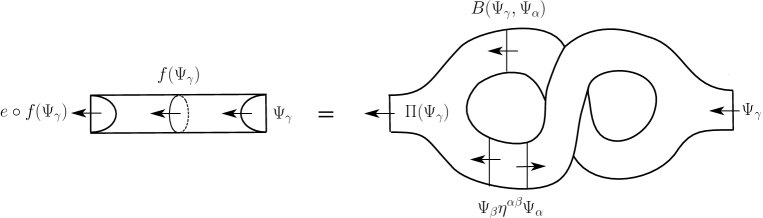
Figure 1: The Cardy condition requires that the factorization of the topological annulus amplitude on closed and open string channels yields the same result. We show in the text that its solution is intimately tied to the factorization condition $W=EJ$ of the LG superpotential.

$$\Pi^{(\ell)}(\Psi_{c}(\phi)) = \sum_{a,b}\bigl{(}\;\eta^{ba}B^{(\ell)}(\omega{\tilde{\Psi}}_{b},B^{(\ell)}(\Psi_{c},\Psi_{a}))$$ (87)

$$\;\;-\;\eta^{ba}B^{(\ell)}(\Psi_{b},B^{(\ell)}(\Psi_{c},\omega{\tilde{\Psi}}_{a}))\bigr{)}=0\;.$$

Applied to a fermionic field, equation (85) becomes

$$\Pi^{(\ell)}(\omega{\tilde{\Psi}}_{c}(\phi)) = \sum_{a,b}\bigl{(}\eta^{ba}B^{(\ell)}(\omega{\tilde{\Psi}}_{b},B^{(\ell)}(\omega{\tilde{\Psi}}_{c},\Psi_{a}))+\eta^{ba}B^{(\ell)}(\Psi_{b},B^{(\ell)}(\omega{\tilde{\Psi}}_{c},\omega{\tilde{\Psi}}_{a}))\bigr{)}$$ (88)

$$= 2\;\omega^{2}\,{\tilde{\Psi}}_{c}\sum_{a,b}\eta^{ba}\Psi_{a}{\tilde{\Psi}}_{b}\quad\textrm{mod}\quad G^{(\ell)}\;,$$

and using relation $\sum_{a,b}\eta^{ab}\Psi_{a}(\phi){\tilde{\Psi}}_{b}(\phi)=G^{(\ell)}{}^{\prime}$ (66) for the flat basis, we obtain

$$\Pi^{(\ell)}(\omega{\tilde{\Psi}}_{c})=(2\,\omega^{2}\,G^{(\ell)}{}^{\prime})\,{\tilde{\Psi}}_{c}\quad\textrm{mod}\quad G^{(\ell)}\;.$$ (89)

The comparison of (86) and (89) shows that the fermionic ring relation (35), $\omega^{2}=p^{(\ell)}q^{(\ell)}$, is a crucial ingredient in order to satisfy the Cardy relation. The other important ingredient, the factorization $W=p^{(\ell)}q^{(\ell)}G^{(\ell)}{}^{2}+$ const., enters the Cardy condition through the adjoint mapping (83).

Before closing this section we want to make a remark on topological sewing constraints for boundary changing operators, since there occur some subtleties. The topological metric (62) for boundary changing operators (47) is generically degenerate. Therefore, the Cardy condition cannot be formulated in terms of the double-twist diagram (85), because it contains explicitly the inverse metric. Moreover, one can show that the bulk boundary crossing relation (78) is only satisfied in the sense of Ward identities, i.e., only in correlation functions and not as operator identities. This might suggest a relaxation of some of the axioms [1] for a topological field theory.

4 Categorial description of $B$-type $D$-branes

We know from [9, 10] that $D$-branes can often be mathematically described in the language of categories. The branes, or equivalently the boundary conditions or boundary states, provide the objects of the category, whereas the open strings stretching between the $D$-branes are the morphisms. Direct contact between a mathematical description of this type and a field theoretical approach has been made in [10, 13] in the context of B-type branes on Calabi-Yau manifolds, where it was shown that the derived category of coherent sheaves on a manifold $X$ can be obtained as a category of boundary conditions in the B-type topologically twisted sigma model on $X$. To generalize these ideas to Landau-Ginzburg models, the essential new ingredient that has to be taken into account is the superpotential $W$, or, in other words, a regular function $W$ on $X$.

A mathematical definition of B-branes for such models has been proposed by Kontsevich, as reviewed in [34], and investigated in a physics context in [30]. In this section, we will work out this description of $D$-branes for the open string TFT with superpotential $W=\frac{1}{k+2}\phi^{k+2}+\ldots$, where the dots denote general perturbations; we will find that our results of the previous sections are equivalent to Kontsevich’s in that the underlying relevant cohomologies are isomorphic.

Let us briefly recapitulate the construction of Kontsevich, where we closely follow [34]. The first step is to define a triangulated category $DB_{w}$ for each value $w\in{\mathbb{C}}$. The category of B-type branes is then obtained as the disjoint union of all $DB_{w}$. As shown in [34], only finitely many $w$ contribute to this union, namely only those corresponding to critical points of the superpotential. For our purposes, the relevant variety will be $X={\mathbb{C}}$, which simplifies the general discussion in [34], and the only relevant value for $w$ is $w=0$. The category $DB_{0}$ is then defined in the following way:

The objects

The objects of the category are ordered pairs

$$\overline{P}:=\Bigl{(}\lx@xy@svg{\hbox{\raise 0.0pt\hbox{\kern 8.30452pt\hbox{\ignorespaces\ignorespaces\ignorespaces\hbox{\vtop{\kern 0.0pt\offinterlineskip\halign{\entry@#!@&&\entry@@#!@\cr&\crcr}}}\ignorespaces{\hbox{\kern-8.30452pt\raise 0.0pt\hbox{\hbox{\kern 0.0pt\raise 0.0pt\hbox{\hbox{\kern 3.0pt\raise 0.0pt\hbox{$\textstyle{P_{1}\ignorespaces\ignorespaces\ignorespaces\ignorespaces}$}}}}}}}\ignorespaces\ignorespaces\ignorespaces\ignorespaces{}{\hbox{\lx@xy@droprule}}\ignorespaces\ignorespaces\ignorespaces{\hbox{\kern 14.54358pt\raise 7.77084pt\hbox{{}\hbox{\kern 0.0pt\raise 0.0pt\hbox{\hbox{\kern 3.0pt\hbox{\hbox{\kern 0.0pt\raise-0.8264pt\hbox{$\scriptstyle{p_{1}}$}}}\kern 3.0pt}}}}}}\ignorespaces{\hbox{\kern 32.30452pt\raise 2.58334pt\hbox{\hbox{\kern 0.0pt\raise 0.0pt\hbox{\lx@xy@tip{1}\lx@xy@tip{-1}}}}}}{\hbox{\lx@xy@droprule}}{\hbox{\lx@xy@droprule}}{\hbox{\kern 32.30452pt\raise 0.0pt\hbox{\hbox{\kern 0.0pt\raise 0.0pt\hbox{\hbox{\kern 3.0pt\raise 0.0pt\hbox{$\textstyle{P_{0}\ignorespaces\ignorespaces\ignorespaces\ignorespaces}$}}}}}}}\ignorespaces\ignorespaces\ignorespaces\ignorespaces{}{\hbox{\lx@xy@droprule}}\ignorespaces\ignorespaces\ignorespaces{\hbox{\kern 14.54358pt\raise-7.77083pt\hbox{{}\hbox{\kern 0.0pt\raise 0.0pt\hbox{\hbox{\kern 3.0pt\hbox{\hbox{\kern 0.0pt\raise-0.8264pt\hbox{$\scriptstyle{p_{0}}$}}}\kern 3.0pt}}}}}}\ignorespaces{\hbox{\kern 8.30452pt\raise-2.58334pt\hbox{\hbox{\kern 0.0pt\raise 0.0pt\hbox{\lx@xy@tip{1}\lx@xy@tip{-1}}}}}}{\hbox{\lx@xy@droprule}}{\hbox{\lx@xy@droprule}}\ignorespaces}}}}\ignorespaces\Bigl{)}\;. \textstyle{P_{1}\ignorespaces\ignorespaces\ignorespaces\ignorespaces} \scriptstyle{p_{1}} \textstyle{P_{0}\ignorespaces\ignorespaces\ignorespaces\ignorespaces} \scriptstyle{p_{0}}$$ (90)

In the general case, $P_{0}$ and $P_{1}$ are projective $A$-modules, where $A$ is such that the smooth variety $X$ is obtained as $X=Spec(A)$. In the simple case that we consider, where $X$ is the complex plane, the only relevant projective module corresponds to the structure sheaf ${\cal O}$, so that $P_{0}=P_{1}={\cal O}$. The choice for the maps $p_{0}$, $p_{1}$ is restricted by the requirement that their composition is the multiplication by $W$. As we will see, they correspond to the polynomials $E$ and $J$ in (25).

The morphisms

The morphisms of the category are given by

$$Hom(\overline{P},\overline{Q})=\bigoplus_{i,j}Hom(P_{i},Q_{j}),$$ (91)

subject to the restriction that they are closed with respect to a differential operator $D$, and taken modulo $D$-exact operators. We define the differential $D$ acting on a morphism $f\in Hom(P_{i},Q_{j})$ by

$$Df=q\circ f-(-1)^{k}f\circ p.$$ (92)

Here, $k$ is a ${\mathbb{Z}}_{2}$ grade of $f$, given by $i-j$. We refer to degree $0$ operators as bosons and to degree $1$ operators as fermions. The differential maps even to odd morphisms, i.e. is itself an odd operator, as it should be.

To determine the open string spectrum on a $D$-brane in the language of categories, we will now spell out explicitly the conditions for an operator to be physical. A bosonic operator $f$, which maps $\overline{P}\to\overline{Q}$, consists of two components $f=(f_{0},f_{1})$, where $f_{0}:P_{0}\to Q_{0}$ and $f_{1}:P_{1}\to Q_{1}$. The differential $D$ acts as

$$Df=\left(\begin{array}[]{c}q_{0}f_{0}-f_{1}p_{0}\\ q_{1}f_{1}-f_{0}p_{1}\end{array}\right)\ ,$$ (93)

and this implies in particular that the condition $Df=0$ can be formulated in terms of the components as

$$q_{1}f_{1}=f_{0}p_{1},\quad q_{0}f_{0}=f_{1}p_{0}.$$ (94)

Likewise, a fermionic operator $t$ has two components, $t=(t_{0},t_{1})$, where $t_{0}:P_{0}\to Q_{1}$ and $t_{1}:P_{1}\to Q_{0}$. The differential acts on the fermions as

$$Dt=\left(\begin{array}[]{c}q_{1}t_{0}+t_{1}p_{0}\\ q_{0}t_{1}+t_{0}p_{1}\end{array}\right)\ .$$ (95)

For the bosonic spectrum, we thus want to divide out the operators that can be written as

$$f_{0} = q_{1}t_{0}+t_{1}p_{0}\ ,$$

$$f_{1} = q_{0}t_{1}+t_{0}p_{1}.$$ (96)

The conditions for a fermionic operator $(s_{0},s_{1})$ to be in the physical spectrum are

$$q_{1}s_{0}=-s_{1}p_{0},\quad q_{0}s_{1}=-s_{0}p_{1},$$ (97)

modulo the operators that are derivatives of a boson $(g_{0},g_{1})$

$$s_{0} = q_{0}g_{0}-g_{1}q_{0}\ ,$$

$$s_{1} = q_{1}g_{1}-g_{0}p_{1}\ .$$ (98)

It is sometimes useful to summarize the operators in matrix notation in the following way:

$${\cal F}_{\overline{P}\overline{Q}}=\left(\begin{array}[]{cc}f_{0}&0\\ 0&f_{1}\end{array}\right),\quad{\cal S}_{\overline{P}\overline{Q}}=\left(\begin{array}[]{cc}0&s_{1}\\ s_{0}&0\end{array}\right)\ .$$ (99)

Here, ${\cal F}$ and ${\cal S}$ are bosonic and fermionic operators, respectively, and it is understood that $f_{0}$ maps $P_{0}$ to $Q_{0}$, $f_{1}:P_{1}\to Q_{1}$, $s_{0}:P_{0}\to Q_{1}$ and $s_{1}:P_{1}\to Q_{0}$. The matrix multiplication is then compatible with the composition of operators. It is possible to represent also the derivative $D$ in terms of matrices. For this, define

$${\cal Q}=\left(\begin{array}[]{cc}0&q_{1}\\ q_{0}&0\end{array}\right),\quad{\cal P}=\left(\begin{array}[]{cc}0&p_{1}\\ p_{0}&0\end{array}\right),\quad\epsilon=\left(\begin{array}[]{cc}1&0\\ 0&-1\end{array}\right).$$ (100)

The derivative acting on a matrix ${\cal F}$ can then be expressed as

$$D{\cal F}_{\overline{P}\overline{Q}}={\cal Q}{\cal F}_{\overline{P}\overline{Q}}-\epsilon{\cal F}_{\overline{P}\overline{Q}}\epsilon{\cal P}\ .$$ (101)

Since the category $DB_{0}$ is triangulated, there exists a translation functor denoted by “$[1]$”, or, in physics language, a notion of an anti-brane. It is defined by

$$\overline{P}[1]=\lx@xy@svg{\hbox{\raise 0.0pt\hbox{\kern 11.41563pt\hbox{\ignorespaces\ignorespaces\ignorespaces\hbox{\vtop{\kern 0.0pt\offinterlineskip\halign{\entry@#!@&&\entry@@#!@\cr&\crcr}}}\ignorespaces{\hbox{\kern-11.41563pt\raise 0.0pt\hbox{\hbox{\kern 0.0pt\raise 0.0pt\hbox{\hbox{\kern 3.0pt\raise 0.0pt\hbox{$\textstyle{\Bigl{(}P_{0}\ignorespaces\ignorespaces\ignorespaces\ignorespaces}$}}}}}}}\ignorespaces\ignorespaces\ignorespaces\ignorespaces{}{\hbox{\lx@xy@droprule}}\ignorespaces\ignorespaces\ignorespaces{\hbox{\kern 14.93248pt\raise 7.77084pt\hbox{{}\hbox{\kern 0.0pt\raise 0.0pt\hbox{\hbox{\kern 3.0pt\hbox{\hbox{\kern 0.0pt\raise-0.8264pt\hbox{$\scriptstyle{-p_{0}}$}}}\kern 3.0pt}}}}}}\ignorespaces{\hbox{\kern 35.41563pt\raise 2.58334pt\hbox{\hbox{\kern 0.0pt\raise 0.0pt\hbox{\lx@xy@tip{1}\lx@xy@tip{-1}}}}}}{\hbox{\lx@xy@droprule}}{\hbox{\lx@xy@droprule}}{\hbox{\kern 35.41563pt\raise 0.0pt\hbox{\hbox{\kern 0.0pt\raise 0.0pt\hbox{\hbox{\kern 3.0pt\raise 0.0pt\hbox{$\textstyle{P_{1}\ignorespaces\ignorespaces\ignorespaces\ignorespaces}$}}}}}}}\ignorespaces\ignorespaces\ignorespaces\ignorespaces{}{\hbox{\lx@xy@droprule}}\ignorespaces\ignorespaces\ignorespaces{\hbox{\kern 14.93248pt\raise-7.77083pt\hbox{{}\hbox{\kern 0.0pt\raise 0.0pt\hbox{\hbox{\kern 3.0pt\hbox{\hbox{\kern 0.0pt\raise-0.8264pt\hbox{$\scriptstyle{-p_{1}}$}}}\kern 3.0pt}}}}}}\ignorespaces{\hbox{\kern 11.41565pt\raise-2.58334pt\hbox{\hbox{\kern 0.0pt\raise 0.0pt\hbox{\lx@xy@tip{1}\lx@xy@tip{-1}}}}}}{\hbox{\lx@xy@droprule}}{\hbox{\lx@xy@droprule}}\ignorespaces}}}}\ignorespaces\Bigl{)}. \textstyle{\Bigl{(}P_{0}\ignorespaces\ignorespaces\ignorespaces\ignorespaces} \scriptstyle{-p_{0}} \textstyle{P_{1}\ignorespaces\ignorespaces\ignorespaces\ignorespaces} \scriptstyle{-p_{1}}$$ (102)

The spectrum of bosonic physical operators between $\overline{P}$ and $\overline{Q}[1]$ coincides with the fermionic part of the spectrum between $\overline{P}$ and $\overline{Q}$. Switching to anti-branes shifts the grade of all operators by one unit.

To give the full data of a triangulated category, we have to define a set of standard triangles in the category. To do so, we first associate to any morphism $f:\overline{P}\to\overline{Q}$ a mapping cone $C(f)$ as an object

$$C(f)=\lx@xy@svg{\hbox{\raise 0.0pt\hbox{\kern 21.7684pt\hbox{\ignorespaces\ignorespaces\ignorespaces\hbox{\vtop{\kern 0.0pt\offinterlineskip\halign{\entry@#!@&&\entry@@#!@\cr&\crcr}}}\ignorespaces{\hbox{\kern-21.7684pt\raise 0.0pt\hbox{\hbox{\kern 0.0pt\raise 0.0pt\hbox{\hbox{\kern 3.0pt\raise 0.0pt\hbox{$\textstyle{\Bigl{(}Q_{1}\oplus P_{0}\ignorespaces\ignorespaces\ignorespaces\ignorespaces}$}}}}}}}\ignorespaces\ignorespaces\ignorespaces\ignorespaces{}{\hbox{\lx@xy@droprule}}\ignorespaces\ignorespaces\ignorespaces{\hbox{\kern 26.6982pt\raise 7.73473pt\hbox{{}\hbox{\kern 0.0pt\raise 0.0pt\hbox{\hbox{\kern 3.0pt\hbox{\hbox{\kern 0.0pt\raise-0.8625pt\hbox{$\scriptstyle{c_{1}}$}}}\kern 3.0pt}}}}}}\ignorespaces{\hbox{\kern 45.7684pt\raise 2.58334pt\hbox{\hbox{\kern 0.0pt\raise 0.0pt\hbox{\lx@xy@tip{1}\lx@xy@tip{-1}}}}}}{\hbox{\lx@xy@droprule}}{\hbox{\lx@xy@droprule}}{\hbox{\kern 45.7684pt\raise 0.0pt\hbox{\hbox{\kern 0.0pt\raise 0.0pt\hbox{\hbox{\kern 3.0pt\raise 0.0pt\hbox{$\textstyle{Q_{0}\oplus P_{1}\ignorespaces\ignorespaces\ignorespaces\ignorespaces}$}}}}}}}\ignorespaces\ignorespaces\ignorespaces\ignorespaces{}{\hbox{\lx@xy@droprule}}\ignorespaces\ignorespaces\ignorespaces{\hbox{\kern 26.69821pt\raise-7.73473pt\hbox{{}\hbox{\kern 0.0pt\raise 0.0pt\hbox{\hbox{\kern 3.0pt\hbox{\hbox{\kern 0.0pt\raise-0.8625pt\hbox{$\scriptstyle{c_{0}}$}}}\kern 3.0pt}}}}}}\ignorespaces{\hbox{\kern 21.7684pt\raise-2.58334pt\hbox{\hbox{\kern 0.0pt\raise 0.0pt\hbox{\lx@xy@tip{1}\lx@xy@tip{-1}}}}}}{\hbox{\lx@xy@droprule}}{\hbox{\lx@xy@droprule}}\ignorespaces}}}}\ignorespaces\Bigl{)}\ , \textstyle{\Bigl{(}Q_{1}\oplus P_{0}\ignorespaces\ignorespaces\ignorespaces\ignorespaces} \scriptstyle{c_{1}} \textstyle{Q_{0}\oplus P_{1}\ignorespaces\ignorespaces\ignorespaces\ignorespaces} \scriptstyle{c_{0}}$$ (103)

such that

$$c_{0}=\begin{pmatrix}q_{0}&f_{1}\\ 0&-p_{1}\end{pmatrix},\qquad c_{1}=\begin{pmatrix}q_{1}&f_{0}\\ 0&-p_{0}\end{pmatrix}.$$ (104)

Then there are maps $g:\overline{Q}\to C(f),\;g=({\rm id},0)$ and $h:C(f)\to\overline{P}[1],\;h=(0,-{\rm id})$, and the standard triangles are given as

$$\overline{P}\stackrel{{\scriptstyle f}}{{\longrightarrow}}\overline{Q}\stackrel{{\scriptstyle g}}{{\longrightarrow}}C(f)\stackrel{{\scriptstyle h}}{{\longrightarrow}}\overline{P}[1].$$ (105)

To make the connection to physics, note that the triangles are the appropriate language to discuss tachyon condensation [13]: The tachyon corresponds to the map $f$, representing an open string state. “Tachyon condensation” means to form the “sum” of two branes $\overline{P}$ and $\overline{Q}$ and to deform by $f$. The result is a single $D$-brane, mathematically described by the cone, $C(f)$. The meaning of the triangle (105) is that $\overline{P}$ and $\overline{Q}$ can combine to give $C(f)$ after tachyon condensation.

Calculation of the spectrum

As already mentioned, for an arbitrary Landau-Ginzburg model in one variable, the only relevant projective module to consider is ${\cal O}$. The maps $p_{0}$ and $p_{1}$ are polynomials whose product is $W$. On a single $D$-brane the derivative $D$ acts on operators that are either purely bosonic or purely fermionic as $D{\cal F}=[{\cal P},{\cal F}]_{\pm}$, where, as usual, one picks the commutator if ${\cal F}$ is bosonic and the anti-commutator if ${\cal F}$ is fermionic.

The condition for $D$-closedness for bosons on a single brane is simply $f_{0}=f_{1}$, so that the bosonic physical operators are diagonal matrices. The matrix multiplication of two bosons reduces to the multiplication of holomorphic polynomials $f_{0}$ in one variable $z$. Polynomials of the type $f_{0}=t_{0}p_{1}+t_{1}p_{0}$, where $t_{0},t_{1}$ are arbitrary, are divided out. To solve for the cohomology, let us decompose $p_{0}$ and $p_{1}$ as

$$p_{0}=G^{p_{0}p_{1}}\hat{p}_{0}^{p_{1}},\quad\quad p_{1}=G^{p_{0}p_{1}}\hat{p}_{1}^{p_{0}},$$ (106)

where $G^{p_{0}p_{1}}$ is the greatest common divisor of $p_{0}$, $p_{1}$. One can then see that $f_{0}$ has to be taken modulo $G^{p_{0}p_{1}}$.

For the fermions, $D$-closedness means that $p_{1}s_{0}=-p_{0}s_{1}$, where, according to (98), $s_{0}$ has to be taken modulo $p_{0}$, and $s_{1}$ is defined modulo $p_{1}$. It follows immediately that if one has two fermionic solutions to these equations, they can only differ by multiplication by a diagonal matrix. Hence, all physical fermions are of the form $\omega p(z)$, where $\omega$ is a solution to the constraint equation for the fermions and $p(z)$ a polynomial in $z$ corresponding to a physical boson. We can thus write the following expression for $\omega$

$$\omega=\alpha\left(\begin{array}[]{cc}0&-\hat{p}_{1}^{p_{0}}\\ \hat{p}_{0}^{p_{1}}&0\end{array}\right)$$ (107)

Notice that the computation of the cohomology we have just outlined is strongly reminiscent of the computation in the boundary LG theory, presented in section 3.2. To show that these computations are in fact isomorphic, observe that

$$D\left(\begin{array}[]{cc}0&0\\ 1&0\end{array}\right)=p_{1},\quad D\left(\begin{array}[]{cc}0&1\\ 0&0\end{array}\right)=p_{0},$$ (108)

which reproduces (30) if we identify

$${\cal P}=\sqrt{i}Q,\quad\pi=\left(\begin{array}[]{cc}0&0\\ \sqrt{i}&0\end{array}\right),\quad\bar{\pi}=\left(\begin{array}[]{cc}0&-i\sqrt{i}\\ 0&0\end{array}\right),\quad p_{0}=J,\quad p_{1}=E.$$ (109)

If we set $\alpha=i$ in (107) and use the above identification we get back the expression (33). This shows explicitly that the cohomology problem of the Kontsevich approach is exactly the same as the one encountered in the Landau-Ginzburg formulation. Therefore, the spectrum necessarily agrees in the two formulations.

The same holds for the boundary changing operators: since at this point we can map the cohomology problem to the equivalent problem in the Lagrangian approach, we omit an explicit analysis of those operators in the language of categories.

To recover the structure of the boundary rings discussed in earlier sections, note that “taking the o.p.e.” corresponds to the composition of morphisms. In this way, the Kontsevich approach reproduces the boundary structure constants in the second line of (57).

The restriction to $W=z^{k+2}$

Although it is clear from the above arguments that the spectrum of boundary preserving and boundary changing operators for the special case $W=z^{k+2}$ agrees exactly with the one obtained from the LG theory, we find it an instructive exercise to explicitly work out the full spectrum for this simple case. To specify boundary conditions, we choose $p_{1}=z^{\mu}$, which determines $p_{0}=z^{k+2-\mu}$. The bosonic open string spectrum between the brane $\overline{P}$ with $(p_{0},p_{1})=(z^{k+2-\mu},z^{\mu})$ and the brane $\overline{Q}$ with $(q_{0},q_{1})=(z^{k+2-\nu},z^{\nu})$ is determined using (94), which becomes

$$f_{1}z^{k+2-\mu}=f_{0}z^{k+2-\nu},\quad f_{0}z^{\mu}=z^{\nu}f_{1},$$

which is to be taken modulo

$$f_{0} = t_{0}z^{k+2-\mu}+t_{1}z^{\nu}$$

$$f_{1} = t_{0}z^{k+2-\nu}+t_{1}z^{\mu}\ .$$

Evaluating these conditions, we conclude that for $\mu\geq\nu$ the physical operators are

$$\left(\begin{array}[]{cc}f_{0}&0\\ 0&f_{1}\end{array}\right)_{l}=\left(\begin{array}[]{cc}z^{l}&0\\ 0&z^{l+\mu-\nu}\end{array}\right)\ .$$ (110)

Here, $l$ can take the values $l=0,\dots,\min\{\nu,k+2-\mu\}-1=\min\{\nu,\mu,k+2-\nu,k+2-\mu\}-1$. Similarly, for $\mu\leq\nu$ we get

$$\left(\begin{array}[]{cc}f_{0}&0\\ 0&f_{1}\end{array}\right)_{l}=\left(\begin{array}[]{cc}z^{l-\mu+\nu}&0\\ 0&z^{l}\end{array}\right),$$ (111)

where $l$ can take the values $0,\dots,\min\{\mu,k+2-\nu\}-1=\min\{\nu,\mu,k+2-\nu,k+2-\mu\}-1$. A similar analysis for the fermions leads to the following spectrum of operators:

$$\left(\begin{array}[]{cc}0&s_{1}\\ s_{0}&0\end{array}\right)_{l}=\left(\begin{array}[]{cc}0&-z^{l+\mu+\nu-k-2}\\ z^{l}&0\end{array}\right),\quad l=0,\dots,\min\{k+2-\mu,k+2-\nu\}-1\;,$$ (112)

for $\mu+\nu\geq k+2$ or

$$\left(\begin{array}[]{cc}0&s_{1}\\ s_{0}&0\end{array}\right)_{l}=\left(\begin{array}[]{cc}0&z^{l}\\ -z^{l+k+2-(\mu+\nu)}&0\end{array}\right),\quad l=0,\dots,\min\{\mu,\nu\}-1\;,$$ (113)

for $\mu+\nu\leq k+2$. The spectrum obtained in this way agrees perfectly with the one obtained from the boundary Landau-Ginzburg model (setting $\mu=\ell_{1}\!+\!1$ and $\nu=\ell_{2}\!+\!1$), as well as with the boundary conformal field theory results summarized in Appendix A below.

Appendix A: Boundary spectrum of minimal models from CFT

The $N=2$ minimal model can be realized as an $SU(2)$ WZW model and a Dirac fermion, coupled through a $U(1)$ gauge field. The symmetry group is ${\mathbb{Z}}_{2k+4}\times{\mathbb{Z}}_{2}$, where ${\mathbb{Z}}_{2k+4}$ is an axial $R$-rotation whose generator is denoted by $a$ and ${\mathbb{Z}}_{2}$ is the fermion number $(-1)^{F}$. Taking the orbifold by $(-1)^{F}$ (a non-chiral GSO-projection) one obtains the rational conformal field theory $SU(2)_{k}\times U(1)_{2}/U(1)_{k+2}$. Its $D$-branes can be studied using standard BCFT techniques; their relation to geometry has been studied in [20, 39, 40].

In order to compare with the results of the present paper obtained from the LG model, we are interested to obtain the spectrum on B-type $D$-branes in the $unprojected$ theory, including the statistics of the boundary operators. Starting from the B-type boundary states of the rational model, one first has to undo the GSO projection to obtain the boundary states in the unprojected theory. One can then identify the action of $a$ and $(-1)^{F}$ in the open string sector; the latter in particular determines the statistics. These steps have been performed in [33], and we refer to that paper for a detailed discussion. For completeness, we summarize the main steps and the result.

The primary fields of the rational model are labeled by the triple $(l,m,s)$ where $l\in\{0,1,2,...,k\}$, $m$ is an integer modulo $2k+4$, and $s$ is an integer modulo 4. The NS sectors are defined by $s=0,2$ and the R sectors by $s=-1,1$. We also have the identification $(l,m,s)\sim(k-l,m+k+2,s+2)$ and the selection rule $l+m+s=0$ mod 2. The chiral primary (antichiral primary) states in the NS sector are labeled by $(l,l,0$) ($(l,-l,0)$) if we use the identification in order to set $s=0$. The symmetry group of the model is ${\mathbb{Z}}_{4k+8}$ (generated by the simple current $(0,1,1)$) for $k$ odd and ${\mathbb{Z}}_{2k+4}\times{\mathbb{Z}}_{2}$ (generated by $(0,1,1)$ and $(0,0,2)$) for $k$ even. The current $(0,0,2)$ distinguishes the R and NS sectors of the theory and can be viewed as the quantum symmetry of $(-1)^{F}$.

The Cardy states (A-type boundary states) $|L,M,S\rangle_{C}$ are labeled by the same set $(L,M,S)$ as the primary states. B-type boundary states can be constructed using the fact that one can obtain the diagonal form of the charge conjugation modular invariant by taking a ${\mathbb{Z}}_{k+2}\times{\mathbb{Z}}_{2}$ orbifold. Hence, taking ${\mathbb{Z}}_{k+2}\times{\mathbb{Z}}_{2}$ orbits of A-type states plus an application of the “mirror map” (charge conjugation on the left-movers) leads to B-type boundary states. The ${\mathbb{Z}}_{k+2}$ acts on the Cardy states by shifting $M$ by $2$ and the ${\mathbb{Z}}_{2}$ acts by shifting $S$ by $2$. We therefore label B-type states by the orbit labels $L=\{0,1,2,...,[\frac{k}{2}]\}$, $M=0$ and $S=0,1$. All of these states are purely in the NSNS sector, and these branes are unoriented. A special case arises for the case $k$ even and $L=\frac{k}{2}$ (this observation traces back to [41]). In this case the orbit boundary state is not elementary but can be decomposed further: There are altogether four states $|B,\frac{k}{2},\hat{S}\rangle$ with $\hat{S}=-1,0,1,2$, which are linear combination of an “orbit” NSNS part $|B,\frac{k}{2},S\rangle$ (where $S$ is the mod $2$ reduction of $\hat{S}$) and an extra RR piece. In particular, these branes are oriented. We refer to [40] for details of the construction.

The task is now to resolve the GSO projection to obtain the branes of the unprojected theory. As explained in [33], the unoriented branes remain the same in the projected and unprojected theory. On the other hand, the oriented (short orbit) branes get re-decomposed into a NSNS and an RR part. In this paper, we have developed a LG formulation of the unoriented orbit-type branes, and we point out that a LG interpretation of the oriented B-type branes has been proposed by the authors of [7].

The open string spectrum between the unoriented branes can be obtained as

$${\cal H}_{(L,S)(L^{\prime},S^{\prime})}=\bigoplus_{l+m+s\,{\rm even}}N_{LL^{\prime}}^{l}\Scr{H}^{N=2}_{l,m,S-S^{\prime}},$$ (A.1)

where $N_{LL^{\prime}}^{l}$ are the $SU(2)_{k}$ fusion rule coefficients. The spaces ${\Scr H}^{N=2}_{l,m,[s]}$ are the modules of the unprojected $N=2$ theory, which can be written in terms of the GSO-projected modules as ${\Scr H}^{N=2}_{l,m,[s]}={\Scr H}_{l,m,s}+{\Scr H}_{l,m,s+2}$. $[s]$ denotes the mod $2$ reduction of $s$ and distinguishes NS and R sectors. (Note that $S$ and $S^{\prime}$ in (A.1) were only defined mod $2$, therefore $[S-S^{\prime}]=S-S^{\prime}$ and the bracket can be omitted.)

Since these boundary states are purely in the NSNS sector, it is clear from the closed string sector that the Witten index between them vanishes. For the R-ground states in the open string sector this means that their contributions to ${\rm tr}(-1)^{F}$ cancel out, in other words, half of the supersymmetric $R$ ground states are bosonic, and half of them are fermionic. More precisely, one can see that on a $(L,S)(L^{\prime},S\!+\!1)$-brane pair the ground states from ${\Scr H}^{N=2}_{l,l+1,1}$ and ${\Scr H}^{N=2}_{l,-l-1,1}$ (which is an element of the Hilbert space ${\Scr H}_{l,-l-1,-1}$ of the GSO-projected theory) contribute with opposite sign [33].

By spectral flow $(0,\!-\!1,\!-\!1)$ these representations are related to ${\Scr H}^{N=2}_{l,l,0}$ . Note however that the spectral flow operator is not part of the spectrum of a single brane: RR ground states only propagate if $S-S^{\prime}=1$ mod $2$ and NSNS states only if $S-S^{\prime}=0$ mod $2$. In particular, there are never RR states on a single brane. It is natural to assume that the NSNS chiral primaries split up into a set of bosonic and fermions just as their RR counter parts, which propagate between branes with appropriately shifted label $S$.

To be explicit, the chiral ring consists of elements with charges ($\tilde{q}=q\,(k\!+\!2)$)

$$\begin{array}[]{l@{\;\;\in\;\;}l@{\quad\mathrm{in}\;\;}l}\tilde{q}=l&\left\{|L\!-\!L^{\prime}|,\ |L\!-\!L^{\prime}|\!+\!2,\ \ldots,\ (L\!+\!L^{\prime})\right\}&\;{\Scr H}^{N=2}_{l,l,0}\;,\\[2.84526pt] \tilde{q}=k\!-\!l&\left\{k\!-\!(L\!+\!L^{\prime}),\ k\!-\!(L\!+\!L^{\prime})\!+\!2,\ \ldots,\ k\!-\!|L\!-\!L^{\prime}|\right\}&\;{\Scr H}^{N=2}_{l,-l-2,2}\;,\end{array}$$ (A.4)

where the states of ${\Scr H}^{N=2}_{l,l,0}$ have opposite fermion number parity as compared with the states of ${\Scr H}^{N=2}_{l,-l-2,2}$. This spectrum coincides precisely with the one listed in Tables 1 and 2, as obtained from the unperturbed Landau-Ginzburg theory; the label $L$ of the BCFT formulation corresponds to $\ell$ in the LG formulation.

References

- [1] C. I. Lazaroiu, “On the structure of open-closed topological field theory in two dimensions,” Nucl. Phys. B603 (2001) 497–530, \hrefhttp://www.arxiv.org/abs/hep-th/0010269hep-th/0010269.
- [2] G. Moore and G. Segal, “unpublished,” see lectures by G. Moore at http://online.itp.ucsb.edu/online/mp01.
- [3] G. Moore, “Some comments on branes, G-flux, and K-theory,” Int. J. Mod. Phys. A16 (2001) 936–944, \hrefhttp://www.arxiv.org/abs/hep-th/0012007hep-th/0012007.
- [4] S. M. Natanzon, “Extention cohomological fields theory and noncommutative Frobenius manifolds,” \hrefhttp://www.arxiv.org/abs/math-ph/0206033math-ph/0206033.
- [5] C. Hofman and W.-K. Ma, “Deformations of topological open strings,” JHEP 01 (2001) 035, \hrefhttp://www.arxiv.org/abs/hep-th/0006120hep-th/0006120.
- [6] C. Hofman, “On the open-closed B-model,” \hrefhttp://www.arxiv.org/abs/hep-th/0204157hep-th/0204157.
- [7] K. Hori, S. Katz, A. Klemm, R. Pandharipande, R. Thomas, R. Vakil, and E. Zaslow, “Mirror Symmetry,” to be published in AMS/CMI.
- [8] W. Lerche, P. Mayr, and N. Warner, “N = 1 special geometry, mixed Hodge variations and toric geometry,” \hrefhttp://www.arxiv.org/abs/hep-th/0208039hep-th/0208039.
- [9] M. Kontsevich, “Homological algebra of mirror symmetry,” \hrefhttp://www.arxiv.org/abs/alg-geom/9411018alg-geom/9411018.
- [10] M. R. Douglas, “D-branes, categories and N = 1 supersymmetry,” J. Math. Phys. 42 (2001) 2818–2843, \hrefhttp://www.arxiv.org/abs/hep-th/0011017hep-th/0011017.
- [11] C. I. Lazaroiu, “Generalized complexes and string field theory,” JHEP 06 (2001) 052, \hrefhttp://www.arxiv.org/abs/hep-th/0102122hep-th/0102122.
- [12] C. I. Lazaroiu, “Unitarity, D-brane dynamics and D-brane categories,” JHEP 12 (2001) 031, \hrefhttp://www.arxiv.org/abs/hep-th/0102183hep-th/0102183.
- [13] P. S. Aspinwall and A. E. Lawrence, “Derived categories and zero-brane stability,” JHEP 08 (2001) 004, \hrefhttp://www.arxiv.org/abs/hep-th/0104147hep-th/0104147.
- [14] D.-E. Diaconescu, “Enhanced D-brane categories from string field theory,” JHEP 06 (2001) 016, \hrefhttp://www.arxiv.org/abs/hep-th/0104200hep-th/0104200.
- [15] P. S. Aspinwall and M. R. Douglas, “D-brane stability and monodromy,” JHEP 05 (2002) 031, \hrefhttp://www.arxiv.org/abs/hep-th/0110071hep-th/0110071.
- [16] J. Distler, H. Jockers, and H.-j. Park, “D-brane monodromies, derived categories and boundary linear sigma models,” \hrefhttp://www.arxiv.org/abs/hep-th/0206242hep-th/0206242.
- [17] S. Katz and E. Sharpe, “D-branes, open string vertex operators, and Ext groups,” \hrefhttp://www.arxiv.org/abs/hep-th/0208104hep-th/0208104.
- [18] C. I. Lazaroiu, “D-brane categories,” \hrefhttp://www.arxiv.org/abs/hep-th/0305095hep-th/0305095.
- [19] S. Govindarajan and T. Jayaraman, “On the Landau-Ginzburg description of boundary CFTs and special Lagrangian submanifolds,” JHEP 07 (2000) 016, \hrefhttp://www.arxiv.org/abs/hep-th/0003242hep-th/0003242.
- [20] K. Hori, A. Iqbal, and C. Vafa, “D-branes and mirror symmetry,” \hrefhttp://www.arxiv.org/abs/hep-th/0005247hep-th/0005247.
- [21] S. Govindarajan and T. Jayaraman, “Boundary fermions, coherent sheaves and D-branes on Calabi-Yau manifolds,” Nucl. Phys. B618 (2001) 50–80, \hrefhttp://www.arxiv.org/abs/hep-th/0104126hep-th/0104126.
- [22] K. Hori, “Linear models of supersymmetric D-branes,” \hrefhttp://www.arxiv.org/abs/hep-th/0012179hep-th/0012179.
- [23] P. Mayr, “Phases of supersymmetric D-branes on Kähler manifolds and the McKay correspondence,” JHEP 01 (2001) 018, \hrefhttp://www.arxiv.org/abs/hep-th/0010223hep-th/0010223.
- [24] S. Hellerman and J. McGreevy, “Linear sigma model toolshed for D-brane physics,” JHEP 10 (2001) 002, \hrefhttp://www.arxiv.org/abs/hep-th/0104100hep-th/0104100.
- [25] S. Govindarajan, T. Jayaraman, and T. Sarkar, “On D-branes from gauged linear sigma models,” Nucl. Phys. B593 (2001) 155–182, \hrefhttp://www.arxiv.org/abs/hep-th/0007075hep-th/0007075.
- [26] S. Hellerman, S. Kachru, A. E. Lawrence, and J. McGreevy, “Linear sigma models for open strings,” JHEP 07 (2002) 002, \hrefhttp://www.arxiv.org/abs/hep-th/0109069hep-th/0109069.
- [27] R. Dijkgraaf, H. Verlinde, and E. Verlinde, “Topological strings in ,” Nucl. Phys. B352 (1991) 59–86.
- [28] S. Cecotti and C. Vafa, “Topological antitopological fusion,” Nucl. Phys. B367 (1991) 359–461.
- [29] S. Cecotti and C. Vafa, “Ising model and N=2 supersymmetric theories,” Commun. Math. Phys. 157 (1993) 139–178, \hrefhttp://www.arxiv.org/abs/hep-th/9209085hep-th/9209085.
- [30] A. Kapustin and Y. Li, “D-branes in Landau-Ginzburg models and algebraic geometry,” \hrefhttp://www.arxiv.org/abs/hep-th/0210296hep-th/0210296.
- [31] A. Recknagel and V. Schomerus, “D-branes in Gepner models,” Nucl. Phys. B531 (1998) 185–225, \hrefhttp://www.arxiv.org/abs/hep-th/9712186hep-th/9712186.
- [32] J. Fuchs and C. Schweigert, “Branes: From free fields to general backgrounds,” Nucl. Phys. B530 (1998) 99–136, \hrefhttp://www.arxiv.org/abs/hep-th/9712257hep-th/9712257.
- [33] I. Brunner and K. Hori, “Orientifolds and mirror symmetry,” \hrefhttp://www.arxiv.org/abs/hep-th/0303135hep-th/0303135.
- [34] D. Orlov, “Triangulated categories of singularities and D-branes in Landau-Ginzburg models,” \hrefhttp://www.arxiv.org/abs/math.ag/0302304math.ag/0302304.
- [35] N. P. Warner, “Supersymmetry in boundary integrable models,” Nucl. Phys. B450 (1995) 663–694, \hrefhttp://www.arxiv.org/abs/hep-th/9506064hep-th/9506064.
- [36] H. Ooguri, Y. Oz, and Z. Yin, “D-branes on Calabi-Yau spaces and their mirrors,” Nucl. Phys. B477 (1996) 407–430, \hrefhttp://www.arxiv.org/abs/hep-th/9606112hep-th/9606112.
- [37] W. Lerche, C. Vafa, and N. P. Warner, “Chiral rings in N=2 superconformal theories,” Nucl. Phys. B324 (1989) 427.
- [38] J. Ishida and A. Hosoya, “Path integral for a color spin and path ordered phase factor,” Prog. Theor. Phys. 62 (1979) 544.
- [39] W. Lerche, C. A. Lütken, and C. Schweigert, “D-branes on ALE spaces and the ADE classification of conformal field theories,” Nucl. Phys. B622 (2002) 269–278, \hrefhttp://www.arxiv.org/abs/hep-th/0006247hep-th/0006247.
- [40] J. M. Maldacena, G. W. Moore, and N. Seiberg, “Geometrical interpretation of D-branes in gauged WZW models,” JHEP 07 (2001) 046, \hrefhttp://www.arxiv.org/abs/hep-th/0105038hep-th/0105038.
- [41] G. Pradisi, A. Sagnotti, and Y. S. Stanev, “Completeness conditions for boundary operators in 2d conformal field theory,” Phys. Lett. B381 (1996) 97–104, \hrefhttp://www.arxiv.org/abs/hep-th/9603097hep-th/9603097.