UT-03-15

hep-th/0305103

May, 2003

Level-Expansion Analysis in
NS Superstring Field Theory Revisited

Kazuki Ohmori
Department of Physics, Faculty of Science, University of Tokyo
Hongo 7-3-1, Bunkyo-ku, Tokyo 113-0033, Japan

We study the level-expansion structure of the NS string field theory actions, mainly focusing on the modified (i.e. 0-picture in the NS sector) cubic superstring field theory. This theory has a non-trivial structure already at the quadratic level due to presence of the picture-changing operator. It is explicitly shown how the usual Maxwell and tachyon actions can be obtained after integrating out the auxiliary fields. We then discuss the reality of the action in the CFT language for all of modified cubic, Witten’s cubic and Berkovits’ non-polynomial theories. The tachyon condensation problems in modified cubic theory are re-examined. We also carry out level truncation analysis in vacuum superstring field theory proposed in our previous paper, and find some difficulties in both of cubic and non-polynomial formulations.

1 Introduction

The construction of covariant open superstring field theory based on the RNS formalism [1] has been a long-standing problem due to the complications coming from the concept of ‘picture’. In Witten’s original proposal [2] for cubic superstring field theory, which was the natural extension of his bosonic cubic string field theory [3], the NS string field was taken to be in the ‘natural’ $-1$-picture. However, it turned out that this theory suffered from contact-term divergences at the tree-level caused by the colliding picture-changing operators [4]. About 10 years later, Berkovits found a way to construct a gauge-invariant NS open string field theory action without making use of the picture-changing operators [5]. However, it has been realized that it is impossible to include the Ramond (R) sector string field in the action in a manifestly ten-dimensional Lorentz covariant manner without introducing the picture-changing operations [6]. Furthermore, its ten-dimensional supersymmetric structure still remains unclear.

Before Berkovits’ discovery, in 1990 more conservative method of modifying Witten’s cubic theory had been proposed [8, 9, 10]. There, the NS string field was defined to carry picture number 0 so that the quadratic vertex had the same picture-changing operator insertion as the cubic vertex. In spite of containing the picture-changing operators in the action, it was shown [9, 10] that this theory is free from contact-term divergence problems. With the help of picture-changing operators, we are able not only to include the R sector string field of picture number $-\frac{1}{2}$ in a ten-dimensional Lorentz covariant manner, but also to construct the $d=10$, $\mathcal{N}=1$ spacetime supersymmetry generator. However, a subtle problem regarding the picture-changing operator still remains: The linearized equation of motion $Y_{-2}Q_{B}A=0$ for the NS string field can differ from the usual one $Q_{B}A=0$ because $Y_{-2}$ has a non-trivial kernel. But since the picture-changing operator is inserted at the open string midpoint ($\pm i$ in the UHP representation), $Y_{-2}Q_{B}A=0$ gives the same result as $Q_{B}A=0$ as long as $A$ is restricted to being in the finite-dimensional Fock space. Hence it is conceivable that the level truncation procedure provides an ad hoc way of regularizing the problem of non-trivial kernel of $Y_{-2}$, although the explicit truncation of the states in the kernel of $Y_{-2}$ in the full theory would ruin the associativity of the $*$-product (see e.g. [6, 12]). One of the aims of this paper is to see to what extent the level-truncated modified cubic superstring field theory can reproduce the structure expected of open superstring theory: Action for the low-lying fields, open string tachyon condensation, etc.

This work is also motivated by the desire to investigate the proposed form of vacuum superstring field theory [14] within the level truncation scheme, because no exact D-brane solutions have been found in this theory so far.

Besides, we have found that there have been very few reports on how the reality of the action is guaranteed by imposing appropriate conditions on the string fields. We will answer this question using the CFT method for all three proposals for superstring field theory.

This paper is organized as follows. In section 2 we calculate the cubic superstring field theory action for the NS($+$) massless sector, and show that, even though the $c_{0}L_{0}^{\mathrm{m}}$ term is absent, the correct Maxwell lagrangian can be reproduced after integrating out the auxiliary fields. In section 3 we discuss how to include the NS($-$) states in the action, paying attention to the problem of fixing sign ambiguities. Section 4 is devoted to the discussion about the reality conditions on the string fields. In section 5 we re-examine the non-trivial vacuum solutions previously obtained in the non–GSO-projected [15] and GSO-projected [16] theories in the level truncation scheme, and present a (new) space-dependent kink solution of codimension 1 on a non-BPS D-brane at the lowest level. In section 6 we perform the level-truncation analysis in vacuum superstring field theory. We summarize our results in section 7. The explicit expressions for the component action and technical remarks about the computations involving $X^{\mu}$ are collected in Appendices.

2 NS($+$) Massless Sector

We begin with the detailed study of how the massless gauge field, which belongs to the NS($+$) sector, is described in the modified cubic superstring field theory. Some results have already been shown in the literature [17, 18], but since we are using different conventions from theirs, we will explicitly write them down. The action for the NS($+$) string field $A_{+}$ is given by [8, 9, 10]

$$S=\frac{1}{g_{o}^{2}}\left(\frac{1}{2\alpha^{\prime}}\langle\!\langle Y_{-2}|A_{+},Q_{B}A_{+}\rangle\!\rangle+\frac{1}{3}\langle\!\langle Y_{-2}|A_{+},A_{+}*A_{+}\rangle\!\rangle\right),$$ (2.1)

where $g_{o}$ is the open string coupling constant and the 2- and 3-string vertices are defined as the following correlation functions on the upper half plane,

$$\langle\!\langle Y_{-2}|A_{1},A_{2}\rangle\!\rangle=\lim_{z\to 0}\left\langle Y(i)Y(-i)I\circ A_{1}(z)\ A_{2}(z)\right\rangle_{\mathrm{UHP}},$$ (2.2)

$$\langle\!\langle Y_{-2}|A_{1},A_{2}*A_{3}\rangle\!\rangle=\left\langle Y(i)Y(-i)f^{(3)}_{1}\circ A_{1}(0)f^{(3)}_{2}\circ A_{2}(0)f^{(3)}_{3}\circ A_{3}(0)\right\rangle_{\mathrm{UHP}},$$ (2.3)

where $Y=c\partial\xi e^{-2\phi}$ is the inverse picture-changing operator and $f\circ A(z)$ denotes the conformal transform of the vertex operator $A(z)$ by the conformal map $f$. Concretely, for a primary field $A$ of conformal weight $h$ we have $f\circ A(z)=(f^{\prime}(z))^{h}A(f(z))$. The conformal maps appearing in eqs.(2.2), (2.3) are

$$I(z)=-\frac{1}{z}=h^{-1}(-h(z)),\quad f^{(3)}_{k}(z)=h^{-1}\left(e^{2\pi i\frac{k-2}{3}}h(z)^{2/3}\right),\ \ (k=1,2,3)$$ (2.5)

with

$$h(z)=\frac{1+iz}{1-iz},\quad h^{-1}(z)=-i\frac{z-1}{z+1}.$$

The correlation function is normalized as

$$\left\langle\frac{1}{2}\partial^{2}c\partial cc(x)e^{-2\phi(y)}e^{ikX(w)}\right\rangle_{\mathrm{UHP}}=(2\pi)^{10}\delta^{10}(k),$$ (2.6)

and $(2\pi)^{10}\delta^{10}(0)\equiv V_{10}$ is the volume of the $(9+1)$-dimensional spacetime. The BRST operator $Q_{B}=\oint\frac{dz}{2\pi i}j_{B}(z)$ is nilpotent and acts as a graded derivation in the $*$-algebra. The picture-changing operator $Y_{-2}$ is BRST-invariant in the sense that $[Q_{B},Y_{-2}]=\oint\frac{dz}{2\pi i}j_{B}(z)Y(i)Y(-i)=0$. The 3-string vertex, as well as the $n$-string vertices induced from the repeated use of the $*$-multiplication, satisfies the cyclicity relation

$$\langle\!\langle Y_{-2}|A_{1},A_{2}*A_{3}\rangle\!\rangle=\langle\!\langle Y_{-2}|A_{2},A_{3}*A_{1}\rangle\!\rangle=\langle\!\langle Y_{-2}|A_{3},A_{1}*A_{2}\rangle\!\rangle.$$

It then follows that the action (2.1) is invariant under the gauge transformation

$$\delta A_{+}=\frac{1}{\alpha^{\prime}}Q_{B}\Lambda+A_{+}*\Lambda-\Lambda*A_{+},$$ (2.7)

where $\Lambda$ is an infinitesimal gauge transformation parameter.

It is important to decide whether the overall multiplicative factor in front of the action (2.1) should be positive or negative, because it cannot be absorbed by the redefinition of the real string field. We cannot answer this question at this point, and it should be determined by looking at the sign of the kinetic term of the physical component field, as will be done.

For the superconformal ghost sector, we will entirely be working in the ‘fermionized’ language without referring to the original bosonic $\beta\gamma$-ghost system. But we would like to make a remark on the fermionization formula here. $\beta$ and $\gamma$ are fermionized as

$$\beta=e^{-\phi}(-1)^{-N_{F}}\partial\xi,\quad\gamma=\eta e^{\phi}(-1)^{N_{F}},$$ (2.8)

where

$$N_{F}=\oint\frac{dz}{2\pi i}\left(-:bc:-:\xi\eta:+\sum_{a=0}^{4}:\psi_{a}^{+}\psi_{a}^{-}:\right)$$

and $\psi_{0}^{\pm}=\frac{1}{\sqrt{2}}(\pm\psi_{0}+\psi_{1})$,  $\psi^{\pm}_{a}=\frac{1}{\sqrt{2}}(\psi_{2a}\pm i\psi_{2a+1})\quad(a=1,2,3,4)$. Since $N_{F}$ is an operator that counts the number (mod 2) of the world-sheet fermions $\psi^{\mu},b,c,\xi$ and $\eta$, $\mathit{(-1)^{N_{F}}}$ anticommutes with them. Thus $(-1)^{\pm N_{F}}$ is considered as a cocycle factor attached to $e^{\pm\phi}$ such that $e^{\pm\phi}(-1)^{\pm N_{F}}$ anticommutes with the world-sheet fermions as a whole. The existence of this cocycle factor is important because, if it were absent, the statistics of $\gamma$ and that of $\eta e^{\phi}$ would not agree. From the OPE

$$:e^{q_{1}\phi(z)}::e^{q_{2}\phi(w)}: = (z-w)^{-q_{1}q_{2}}:e^{q_{1}\phi(z)}e^{q_{2}\phi(w)}:$$

$$= (z-w)^{-q_{1}q_{2}}\left(:e^{(q_{1}+q_{2})\phi(w)}:+\mathcal{O}(z-w)\right)$$

one finds that $e^{q_{1}\phi}$ and $e^{q_{2}\phi}$ naturally anticommute with each other when both $q_{1}$ and $q_{2}$ are odd integers. After all, we have found that $e^{q\phi}(-1)^{qN_{F}}$ with odd $q$ anticommutes with all of the fermions and $e^{q^{\prime}\phi}(-1)^{q^{\prime}N_{F}}$ with odd $q^{\prime}$, whereas $e^{q\phi}(-1)^{qN_{F}}$ with even $q=2n$ commutes with everything because $2nN_{F}$ in the NS sector is always an even integer. Therefore, we can abbreviate $e^{q\phi}(-1)^{qN_{F}}$ to $e^{q\phi}$, with the understanding that $e^{q\phi}$ should be treated as a fermion/boson when $q$ is odd/even, respectively. In fact, it appears that almost all the calculations in the literature have been performed using this ‘abbreviation rule’. Also in the rest of this paper we will simply regard $e^{q\phi}$ with odd $q$ as fermionic, instead of explicitly writing the cocycle factor $(-1)^{qN_{F}}$.

We define the ghost number current $j_{\mathrm{gh}}$ and the picture number current $j_{\mathrm{pic}}$ as

$$j_{\mathrm{gh}}=-:bc:-:\xi\eta:,\quad j_{\mathrm{pic}}=:\xi\eta:-\partial\phi.$$ (2.9)

Given the OPEs

$$c(z)b(w)\sim\frac{1}{z-w},\quad\eta(z)\xi(w)\sim\frac{1}{z-w},\quad\phi(z)\phi(w)\sim-\log(z-w),$$ (2.10)

the assignment of the ghost and picture numbers for the ghost fields is found to be

$$\begin{array}[]{|c||c|c|c|c|c|}\hline\cr&b&c&\xi&\eta&e^{q\phi}\\ \hline\cr\#_{\mathrm{gh}}&-1&1&-1&1&0\\ \hline\cr\#_{\mathrm{pic}}&0&0&1&-1&q\\ \hline\cr\end{array}\ .$$

The string field $A_{+}$ is defined to be a Grassmann-odd element in the state space of the 2-dimensional conformal field theory, consisting of states of ghost number 1 and picture number 0. At the massless level, it is expanded as

$$|A_{+}^{(0)}\rangle = A_{+}^{(0)}(0)|0\rangle,$$

$$A_{+}^{(0)}(z) = \int\frac{d^{10}k}{(2\pi)^{10}}\biggl{[}\frac{i}{\sqrt{2\alpha^{\prime}}}A^{1}_{\mu}(k)c\partial X^{\mu}+A^{2}_{\mu}(k)\eta e^{\phi}\psi^{\mu}$$

$${}+\frac{\sqrt{2\alpha^{\prime}}}{2i}F_{\mu\nu}(k)c\psi^{\mu}\psi^{\nu}+iv(k)\partial c+iw(k)c\partial\phi\biggr{]}e^{ikX}(z),$$

where $|0\rangle$ denotes the $SL(2,\mathbb{R})$-invariant vacuum. The reality condition on the string field implies the following reality conditions for the component fields (see section 4 for details),

$$A^{1}_{\mu}(k)^{*}=A^{1}_{\mu}(-k),\quad A^{2}_{\mu}(k)^{*}=A^{2}_{\mu}(-k),\quad F_{\mu\nu}(k)^{*}=F_{\mu\nu}(-k),$$ (2.12)

$$v(k)^{*}=v(-k),\quad w(k)^{*}=w(-k),$$

where ^∗ denotes the complex conjugation.

We will now show the detailed calculations of the quadratic action, i.e. rewriting the action (2.1) in terms of the component fields appearing in (2). In the Abelian case no cubic interactions among the massless fields (2) survive due to the twist symmetry. First, we have to compute the action on $A_{+}^{(0)}$ of the BRST operator

$$Q_{B}=\oint\frac{dz}{2\pi i}\left(cT^{\mathrm{m}}+c\partial\xi\eta+cT^{\phi}+bc\partial c+\eta e^{\phi}G^{\mathrm{m}}-\eta\partial\eta e^{2\phi}b\right),$$ (2.13)

where the energy-momentum tensors $T^{\mathrm{m}},T^{\phi}$ and the matter supercurrent $G^{\mathrm{m}}$ are

$$T^{\mathrm{m}}=-\frac{1}{4\alpha^{\prime}}\partial X^{\mu}\partial X_{\mu}-\frac{1}{2}\psi^{\mu}\partial\psi_{\mu},\qquad T^{\phi}=-\frac{1}{2}\partial\phi\partial\phi-\partial^{2}\phi,\phantom{QQQQQ}$$ (2.14)

$$G^{\mathrm{m}}=\frac{i}{\sqrt{2\alpha^{\prime}}}\partial X^{\mu}\psi_{\mu}.$$

After lengthy calculations we reach

$$Q_{B}|A_{+}^{(0)}\rangle = \int\frac{d^{10}k}{(2\pi)^{10}}\biggl{[}\partial^{2}cc\left(\sqrt{\frac{\alpha^{\prime}}{2}}k^{\mu}A_{\mu}^{1}(k)-iv(k)-iw(k)\right)$$ (2.19)

$${}+\partial cc\partial X^{\mu}\left(i\sqrt{\frac{\alpha^{\prime}}{2}}k^{2}A^{1}_{\mu}(k)+k_{\mu}v(k)\right)$$

$${}+\partial cc\psi^{\mu}\psi^{\nu}\left(-i\alpha^{\prime}k^{2}\sqrt{\frac{\alpha^{\prime}}{2}}F_{\mu\nu}(k)\right)$$

$${}+\partial cc\partial\phi\left(i\alpha^{\prime}k^{2}w(k)\right)$$

$${}+\eta e^{\phi}c\partial\psi^{\mu}\left(-A^{1}_{\mu}(k)+A^{2}_{\mu}(k)-\sqrt{2\alpha^{\prime}}ik_{\mu}w(k)\right)$$

$${}+\eta e^{\phi}c\psi^{\nu}\partial X^{\mu}\left(-ik_{\nu}A^{1}_{\mu}(k)+ik_{\mu}A^{2}_{\nu}(k)-F_{\mu\nu}(k)+\frac{1}{\sqrt{2\alpha^{\prime}}}\eta_{\mu\nu}w(k)\right)$$

$${}+\eta e^{\phi}c\psi^{\rho}\psi^{\mu}\psi^{\nu}\left(i\alpha^{\prime}k_{[\rho}F_{\mu\nu]}(k)\right)$$

$${}+\partial\eta e^{\phi}c\psi^{\mu}\left(-A^{1}_{\mu}(k)+A^{2}_{\mu}(k)-2i\alpha^{\prime}k^{\nu}F_{\mu\nu}(k)-\sqrt{2\alpha^{\prime}}ik_{\mu}w(k)\right)$$

$${}+\eta\partial e^{\phi}c\psi^{\mu}\left(-A^{1}_{\mu}(k)+A^{2}_{\mu}(k)-2i\alpha^{\prime}k^{\nu}F_{\mu\nu}(k)-2\sqrt{2\alpha^{\prime}}ik_{\mu}w(k)\right)$$

$${}+\eta e^{\phi}\partial c\psi^{\mu}\left(\alpha^{\prime}k^{2}A^{2}_{\mu}(k)-\sqrt{2\alpha^{\prime}}ik_{\mu}v(k)\right)$$

$${}+\partial^{2}\eta\eta e^{2\phi}\left(-\sqrt{\frac{\alpha^{\prime}}{2}}k^{\mu}A^{2}_{\mu}(k)+iv(k)+2iw(k)\right)$$

$${}+\partial\eta\eta\partial e^{2\phi}\left(-\sqrt{\frac{\alpha^{\prime}}{2}}k^{\mu}A^{2}_{\mu}(k)+iv(k)+\frac{5}{2}iw(k)\right)$$

$${}+\partial\eta\eta e^{2\phi}\partial X^{\mu}\left(\frac{i}{\sqrt{2\alpha^{\prime}}}(A^{1}_{\mu}(k)-A^{2}_{\mu}(k))\right)$$

$${}+\partial\eta\eta e^{2\phi}\psi^{\mu}\psi^{\nu}\left(\sqrt{2\alpha^{\prime}}k_{[\nu}A^{2}_{\mu]}(k)+\frac{\sqrt{2\alpha^{\prime}}}{2i}F_{\mu\nu}(k)\right)$$

$${}+\partial\eta\eta e^{2\phi}bc(2iw(k))\biggr{]}e^{ikX}(0)|0\rangle,$$

where we have used the OPEs

$$X^{\mu}(z)X^{\nu}(w)\sim-2\alpha^{\prime}\eta^{\mu\nu}\log(z-w),\quad\psi^{\mu}(z)\psi^{\nu}(w)\sim\frac{\eta^{\mu\nu}}{z-w},$$ (2.20)

and eqs.(2.10). _[…] denotes the antisymmetrization operation

$$A_{[\mu}B_{\nu]} = \frac{1}{2!}(A_{\mu}B_{\nu}-A_{\nu}B_{\mu}),$$

$$A_{[\mu}B_{\nu}C_{\rho]} = \frac{1}{3!}(A_{\mu}B_{\nu}C_{\rho}+A_{\nu}B_{\rho}C_{\mu}+A_{\rho}B_{\mu}C_{\nu}-A_{\mu}B_{\rho}C_{\nu}-A_{\nu}B_{\mu}C_{\rho}-A_{\rho}B_{\nu}C_{\mu}).$$

The on-shell conditions are obtained from $Q_{B}|A_{+}^{(0)}\rangle=0$. The full set of resulting 15 equations, however, must be highly redundant because we have only five independent fields. First we choose as four independent equations the non-dynamical ones derived from the expressions (2.19)–(2.19),

$$w(k)=0,\quad A^{1}_{\mu}(k)=A^{2}_{\mu}(k),$$ (2.21)

$$v(k)=-\sqrt{\frac{\alpha^{\prime}}{2}}ik^{\mu}A^{2}_{\mu}(k),$$ (2.22)

$$F_{\mu\nu}(k)=ik_{\mu}A^{2}_{\nu}(k)-ik_{\nu}A^{2}_{\mu}(k),$$ (2.23)

by which the auxiliary fields $w,v,F_{\mu\nu},A^{1}_{\mu}$ can be eliminated. Then the fifth equation from (2.19) implies the Maxwell equation

$$k^{\mu}F_{\mu\nu}(k)=0$$

for the field strength tensor determined in (2.23). One can see that the remaining ten equations are automatically satisfied. Among them is a Bianchi identity $ik_{[\rho}F_{\mu\nu]}=0$.

Let us consider the gauge degree of freedom. The gauge parameter $\Lambda$, which has ghost number 0 and picture number 0, has only one component $\lambda$ at the massless level,

$$\Lambda=\int\frac{d^{10}k}{(2\pi)^{10}}i\sqrt{\frac{\alpha^{\prime}}{2}}\lambda(k)e^{ikX}.$$ (2.24)

At the linearized level, the gauge transformation law (2.7) reduces to

$$\delta A_{+}^{(0)}=\frac{1}{\alpha^{\prime}}Q_{B}\Lambda = \int\frac{d^{10}k}{(2\pi)^{10}}\biggl{(}\frac{i}{\sqrt{2\alpha^{\prime}}}ik_{\mu}\lambda(k)c\partial X^{\mu}$$

$${}+ik_{\mu}\lambda(k)\eta e^{\phi}\psi^{\mu}+i\sqrt{\frac{\alpha^{\prime}}{2}}k^{2}\lambda(k)\partial c\biggr{)}e^{ikX}.$$

Comparing it with the expansion (2), we can read off the gauge transformation law for the component fields:

$$\delta A^{1}_{\mu}(k)=\delta A^{2}_{\mu}(k)=ik_{\mu}\lambda(k),$$

$$\delta v(k)=\sqrt{\frac{\alpha^{\prime}}{2}}k^{2}\lambda(k),\quad\delta F_{\mu\nu}(k)=\delta w(k)=0,$$ (2.26)

which are consistent with the equations of motion. In the Feynman-Siegel gauge $b_{0}|A_{+}\rangle=0$, the coefficient $v$ of $\partial c$ is set to zero. Via the field equation (2.22), $v=0$ means $k^{\mu}A^{2}_{\mu}(k)=0$. Therefore, after eliminating the auxiliary fields using the linearized equations of motion, the Feynman-Siegel gauge condition implies the Lorentz gauge $k^{\mu}A^{2}_{\mu}(k)=0$ for the physical gauge field.

Plugging (2.21)–(2.23) into (2), we get

$$A_{+}^{(0)}(z) = \int\frac{d^{10}k}{(2\pi)^{10}}\Biggl{(}\frac{i}{\sqrt{2\alpha^{\prime}}}A^{2}_{\mu}(k)c\partial X^{\mu}+A^{2}_{\mu}(k)\eta e^{\phi}\psi^{\mu}$$

$${}+\sqrt{2\alpha^{\prime}}k_{[\mu}A^{2}_{\nu]}(k)c\psi^{\mu}\psi^{\nu}+\sqrt{\frac{\alpha^{\prime}}{2}}k^{\mu}A^{2}_{\mu}(k)\partial c\Biggr{)}e^{ikX}(z).$$

This ‘on-shell’ vertex operator in fact coincides with the one obtained by acting with the picture-raising operator

$$\mathrm{X}=c\partial\xi+e^{\phi}G^{\mathrm{m}}+e^{2\phi}b\partial\eta+\partial(e^{2\phi}b\eta)$$ (2.28)

on the massless vertex $V$ in the $-1$ picture,

$$V(w)=\int\frac{d^{10}k}{(2\pi)^{10}}\Bigl{(}-\tilde{A}_{\mu}(k)ce^{-\phi}\psi^{\mu}e^{ikX}(w)-i\tilde{v}(k)c\partial c\partial\xi e^{-2\phi}e^{ikX}(w)\Bigr{)}.$$ (2.29)

Generically, $\displaystyle\lim_{z\to w}\mathrm{X}(z)V(w)$ contains a divergent piece:

$$\mathrm{X}(z)V(w) = \int\frac{d^{10}k}{(2\pi)^{10}}\biggl{[}\frac{1}{z-w}\left(\sqrt{2\alpha^{\prime}}k^{\mu}\tilde{A}_{\mu}(k)-2i\tilde{v}(k)\right)c(w)+\frac{i}{\sqrt{2\alpha^{\prime}}}\tilde{A}_{\mu}(k)c\partial X^{\mu}(w)$$

$${}+\tilde{A}_{\mu}(k)\eta e^{\phi}\psi^{\mu}(w)+\sqrt{2\alpha^{\prime}}k_{[\mu}\tilde{A}_{\nu]}(k)c\psi^{\mu}\psi^{\nu}(w)+i\tilde{v}(k)\partial c(w)$$

$${}+\left(\sqrt{2\alpha^{\prime}}k^{\mu}\tilde{A}_{\mu}(k)-2i\tilde{v}(k)\right)c\partial\phi(w)+\mathcal{O}(z-w)\biggr{]}e^{ikX(w)}.$$

However, this divergent contribution can be removed by setting $\tilde{v}(k)=-\sqrt{\frac{\alpha^{\prime}}{2}}ik^{\mu}\tilde{A}_{\mu}(k)$, which is one of the field equations obtained from the on-shell condition $Q_{B}V=0$. At the same time, the resulting expression agrees with (2) if we identify $\tilde{A}_{\mu}$ with $A^{2}_{\mu}$.

Let us return to the computation of the action. Noting that $\partial X^{\mu}e^{ikX},\partial c$ and $\partial\phi$ are no longer primary fields, we find

$$I\circ A^{(0)}_{+}(z) = \int\frac{d^{10}k}{(2\pi)^{10}}|z^{-2}|^{\alpha^{\prime}k^{2}}\biggl{[}\frac{i}{\sqrt{2\alpha^{\prime}}}A^{1}_{\mu}(k)c\partial X^{\mu}+A^{2}_{\mu}(k)\eta e^{\phi}\psi^{\mu}$$

$${}+\frac{\sqrt{2\alpha^{\prime}}}{2i}F_{\mu\nu}(k)c\psi^{\mu}\psi^{\nu}+iv(k)\partial c+iw(k)c\partial\phi$$

$${}+z\left(-\sqrt{2\alpha^{\prime}}k^{\mu}A^{1}_{\mu}(k)+2iv(k)+2iw(k)\right)c\biggr{]}e^{ikX}\left(-\frac{1}{z}\right).$$

The final step is to substitute the expressions for $Q_{B}A_{+}^{(0)}(z)$ and $I\circ A^{(0)}_{+}(z)$ into

$$\langle\!\langle Y_{-2}|A_{+}^{(0)},Q_{B}A_{+}^{(0)}\rangle\!\rangle=\lim_{z\to 0}\left\langle Y(i)Y(-i)I\circ A^{(0)}_{+}(z)\ Q_{B}A_{+}^{(0)}(z)\right\rangle_{\mathrm{UHP}}$$ (2.32)

and evaluate numerous correlators using the OPEs (2.10), (2.20) and the normalization (2.6). The fully off-shell action for the massless component fields finally becomes

$$S^{(0)} = \frac{1}{2\alpha^{\prime}g_{o}^{2}}\int\frac{d^{10}k}{(2\pi)^{10}}\biggl{[}-\eta^{\mu\nu}A^{1}_{\mu}(-k)A^{2}_{\nu}(k)+\frac{1}{2}\eta^{\mu\nu}A^{1}_{\mu}(-k)A^{1}_{\nu}(k)$$

$${}+\frac{1}{2}\eta^{\mu\nu}A^{2}_{\mu}(-k)A^{2}_{\nu}(k)-2\alpha^{\prime}\eta^{\mu\nu}ik^{\rho}A^{2}_{\mu}(-k)F_{\nu\rho}(k)-\sqrt{2\alpha^{\prime}}ik^{\mu}A^{2}_{\mu}(-k)w(k)$$

$${}+\frac{\alpha^{\prime}}{2}F^{\mu\nu}(-k)F_{\mu\nu}(k)+\frac{5}{2}w(-k)w(k)+2v(-k)w(k)\biggr{]},$$

where $\eta^{\mu\nu}=\mathrm{diag}(-+\ldots+)$ is the spacetime metric. The set of five equations of motion derived by varying the action with respect to the field variables coincides with the previous one which has been found from $Q_{B}A_{+}^{(0)}=0$, as it should be. Surprisingly, the above expression does not contain any contributions from the ‘Klein-Gordon operator’ $c_{0}L_{0}^{\mathrm{m}}\sim\alpha^{\prime}p^{2}$ in $Q_{B}$. From the (anomalous) $\phi$-charge conservation, one may naïvely expect that $\langle\!\langle Y_{-2}|A,\oint\frac{dz}{2\pi i}cT^{\mathrm{m}}A\rangle\!\rangle$ is non-vanishing if $A$ has $\phi$-charge $+1$. However, this correlator actually vanishes for the string field of the form $\eta e^{\phi}\mathcal{V}(X^{\mu},\psi^{\mu})$ with $\mathcal{V}$ denoting an arbitrary vertex operator made out of the matter fields, because $\langle\partial\xi(i)\partial\xi(-i)\eta(-1/z)\eta(z)\rangle_{\xi\eta}=0$ for any $z$. Nevertheless, the usual kinetic term for the physical gauge field $A_{\mu}^{2}$ can be obtained after integrating out the auxiliary fields by their equations of motion:

$$S^{(0)}[A^{2}] = \frac{1}{g_{o}^{2}}\int\frac{d^{10}k}{(2\pi)^{10}}\left(-\frac{1}{4}\mathcal{F}^{\mu\nu}(-k)\mathcal{F}_{\mu\nu}(k)\right)$$ (2.34)

$$= \frac{1}{g_{o}^{2}}\int d^{10}x\left(-\frac{1}{4}\mathcal{F}^{\mu\nu}(x)\mathcal{F}_{\mu\nu}(x)\right),$$

where we have Fourier-transformed to the position space as $\mathcal{F}_{\mu\nu}(k)=\int d^{10}x\mathcal{F}_{\mu\nu}(x)e^{-ikx},$ and $\mathcal{F}_{\mu\nu}$ is the field strength tensor for the gauge potential, $\mathcal{F}_{\mu\nu}(x)=\partial_{\mu}A^{2}_{\nu}(x)-\partial_{\nu}A^{2}_{\mu}(x).$ Needless to say, the action (2.34) is exactly the Maxwell action we are familiar with. Here, we can at last answer the question raised at the beginning of this section: Since the above kinetic term for the gauge field is accompanied by the standard coefficient $-\frac{1}{4}$, we conclude that the sign of the overall multiplicative factor in front of the string field theory action should be plus, as already indicated in eq.(2.1), if we use the normalization convention (2.6) of the correlator.

3 Including the GSO($-$) Tachyon

3.1 Precise definition of the vertices

The defining property of the GSO($-$) states is that they have odd world-sheet spinor numbers, where we assign to $\psi^{\mu},e^{q\phi}$ world-sheet spinor numbers 1 and $q$, respectively. If we restrict ourselves to the subspace of ghost number 1, it then follows that the GSO($-$) string field $A_{-}$ is Grassmann-even and contains states of half-integer–valued conformal weights. First of all, since $A_{-}$ has different Grassmannality from the GSO($+$) string field $A_{+}$, it seems that they fail to obey common algebraic relations. This problem can be resolved by attaching the $2\times 2$ internal Chan-Paton matrices to the string fields and the operator insertions as [20, 21, 22]

$$\widehat{Q}_{B}=Q_{B}\otimes\sigma_{3},\quad\widehat{Y}_{-2}=Y_{-2}\otimes\sigma_{3},$$

$$\widehat{A}=A_{+}\otimes\sigma_{3}+A_{-}\otimes i\sigma_{2}.$$ (3.1)

Due to the fact that $A_{-}$ has half-integer weights $h_{-}$, $A_{-}$ changes its sign under the conformal transformation $\mathcal{R}_{2\pi}$ representing the $2\pi$ rotation of the unit disk, namely

$$\mathcal{R}_{2\pi}\circ A_{-}(z)=(\mathcal{R}_{2\pi}^{\prime}(z))^{h_{-}}A_{-}(\mathcal{R}_{2\pi}(z))=e^{2\pi ih_{-}}A_{-}(z)=-A_{-}(z).$$ (3.2)

This in particular means that an additional minus sign arises in the cyclicity relation,

$$\langle\!\langle Y_{-2}|A_{-},B_{-}\rangle\!\rangle=-\langle\!\langle Y_{-2}|B_{-},A_{-}\rangle\!\rangle,$$ (3.3)

$$\langle\!\langle Y_{-2}|A_{-},B_{1}*B_{2}\rangle\!\rangle=-\langle\!\langle Y_{-2}|B_{1},B_{2}*A_{-}\rangle\!\rangle.$$ (3.4)

Then, the cubic superstring field theory action including both NS($\pm$) string fields can be written as [15, 22]

$$S = \frac{1}{2g_{o}^{2}}\mathrm{Tr}\left[\frac{1}{2\alpha^{\prime}}\langle\!\langle\widehat{Y}_{-2}|\widehat{A},\widehat{Q}_{B}\widehat{A}\rangle\!\rangle+\frac{1}{3}\langle\!\langle\widehat{Y}_{-2}|\widehat{A},\widehat{A}*\widehat{A}\rangle\!\rangle\right]$$

$$= \frac{1}{g_{o}^{2}}\Biggl{[}\frac{1}{2\alpha^{\prime}}\langle\!\langle Y_{-2}|A_{+},Q_{B}A_{+}\rangle\!\rangle+\frac{1}{3}\langle\!\langle Y_{-2}|A_{+},A_{+}*A_{+}\rangle\!\rangle$$

$$\ \ {}+\frac{1}{2\alpha^{\prime}}\langle\!\langle Y_{-2}|A_{-},Q_{B}A_{-}\rangle\!\rangle+\langle\!\langle Y_{-2}|A_{-},A_{+}*A_{-}\rangle\!\rangle\Biggr{]}.$$

However, the last two terms still have sign ambiguities because of the square-roots in the conformal factors

$$(I^{\prime}(z))^{h_{-}},\quad(f^{(3)\prime}_{1}(0))^{h_{-}},\quad(f^{(3)\prime}_{3}(0))^{h_{-}}.$$

The authors of [21] proposed a natural prescription to this problem in the case of the disk representation of the string vertices, and in addition showed how to translate it into the UHP representation:

If the conformal maps $$f^{(n)}_{k} n$$ defining the -string vertex have the property that

all $$f^{(n)}_{k}(0) f^{(n)}_{1}(0)<f^{(n)}_{2}(0)<\ldots<f^{(n)}_{n}(0)$$ are real and satisfy , (3.6)

then we should choose the positive sign for all $$(f^{(n)\prime}_{k}(0))^{1/2}$$.

In this paper we will follow this prescription and write down explicit expressions for the 2- and 3-string vertices. For the 3-string vertex, the prescription (3.6) can immediately be applied because our definition (2.5) of $f^{(3)}_{k}$ satisfies the condition

$$f^{(3)}_{1}(0)=-\sqrt{3}<f^{(3)}_{2}(0)=0<f^{(3)}_{3}(0)=\sqrt{3}.$$

Hence we take

$$(f^{(3)\prime}_{1}(0))^{h_{-}}=(f^{(3)\prime}_{3}(0))^{h_{-}}\equiv\bigg{|}\left(\frac{8}{3}\right)^{h_{-}}\bigg{|}.$$ (3.7)

In the case of the 2-string vertex, however, we have to be more careful. We define $\mathcal{R}_{\theta}$ to be a conformal map corresponding to the rotation of the unit disk by an angle $\theta$,

$$\mathcal{R}_{\theta}(z)=h^{-1}\left(e^{i\theta}h(z)\right),$$ (3.8)

which forms an Abelian subgroup of $SL(2,\mathbb{R})$. Noting that the inversion can be expressed as $I(z)=h^{-1}(e^{-\pi i}h(z))=\mathcal{R}_{-\pi}(z)$, we write the 2-vertex (2.2) as

$$\langle\!\langle Y_{-2}|A,B\rangle\!\rangle=\left\langle Y(i)Y(-i)\ \mathcal{R}_{-\pi}\circ A(0)\ B(0)\right\rangle_{\mathrm{UHP}}.$$ (3.9)

In order to make the above prescription applicable, we use the $SL(2,\mathbb{R})$-invariance of the correlation function to rewrite the 2-vertex in the following way,

$$\langle\!\langle Y_{-2}|A,B\rangle\!\rangle = \lim_{\epsilon\to 0^{+}}\left\langle Y(i)Y(-i)\ \mathcal{R}_{-\pi+2\epsilon}\circ A(0)\ \mathcal{R}_{2\epsilon}\circ B(0)\right\rangle_{\mathrm{UHP}}$$ (3.10)

$$=\lim_{\epsilon\to 0^{+}}(\mathcal{R}^{\prime}_{2\epsilon}(0))^{h_{A}+h_{B}}(\mathcal{R}^{\prime}_{-\pi}(z))^{h_{A}}\left\langle Y(i)Y(-i)A(-1/z)B(z)\right\rangle_{\mathrm{UHP}},$$

where we have defined $z\equiv\mathcal{R}_{2\epsilon}(0)\simeq\epsilon\ (>0)$, and used the (de)composition law $\mathcal{R}_{-\pi+2\epsilon}=\mathcal{R}_{-\pi}\circ\mathcal{R}_{2\epsilon}$. In addition, we have assumed $A,B$ to be primary fields for simplicity. Then, since $f^{(2)}_{1}(0)\equiv\mathcal{R}_{-\pi+2\epsilon}(0)<0<f^{(2)}_{2}(0)\equiv\mathcal{R}_{2\epsilon}(0)$, we can determine the prefactors of (3.10) to be

$$(\mathcal{R}^{\prime}_{2\epsilon}(0))^{h_{A}+h_{B}}(\mathcal{R}^{\prime}_{-\pi}(z))^{h_{A}}=|(\sec\epsilon)^{2(h_{A}+h_{B})}||z^{-2h_{A}}|$$

according to the prescription (3.6). As for the first factor, nothing prevents us from taking the limit $\epsilon\to 0^{+}$ in advance, and it gives a factor of 1. Thus, we have finally found the 2-vertex to be given by

$$\langle\!\langle Y_{-2}|A,B\rangle\!\rangle=\lim_{z\to 0^{+}}\left\langle Y(i)Y(-i)\ \mathcal{R}_{-\pi}\circ A(z)\ B(z)\right\rangle_{\mathrm{UHP}},$$ (3.11)

with the prescription for the conformal factor

$$(\mathcal{R}_{-\pi}^{\prime}(z))^{h}=z^{-2h},$$ (3.12)

where we have used $|z|=z$ under $z\to 0^{+}$. Consistency of the composition law $\mathcal{R}_{\pi}=\mathcal{R}_{-\pi}\circ\mathcal{R}_{2\pi}$ and the action of $\mathcal{R}_{2\pi}$ (3.2) then requires

$$(\mathcal{R}_{\pi}^{\prime}(z))^{h}=e^{2\pi ih}z^{-2h}.$$ (3.13)

For notational simplicity we shall use the conventional symbol $I$ as $I=\mathcal{R}_{-\pi},\ I^{-1}=\mathcal{R}_{\pi}$ with the prescriptions (3.12), (3.13) included. That is to say, we define

$$(I^{\prime}(z))^{h}=z^{-2h},\qquad((I^{-1})^{\prime}(z))^{h}=e^{2\pi ih}z^{-2h}.$$ (3.14)

Notice that $I^{2}\circ\Phi=\mathcal{R}_{-2\pi}\circ\Phi=(-1)^{2h}\Phi$. Once we have found which of the square-root branches we should choose, we no longer need to specify how to take the limit $z\to 0$. To summarize, the 2-vertex is computed as

$$\langle\!\langle Y_{-2}|A,B\rangle\!\rangle=\lim_{z\to 0}\langle Y(i)Y(-i)I\circ A(z)\ B(z)\rangle_{\mathrm{UHP}},$$ (3.15)

with the prescription (3.14).

So far we have had zero-momentum vertex operators in mind. We need some special care for the treatment of the momentum factor $e^{ikX}$, see Appendix B.

3.2 Action for the tachyons

In the space of ghost number 1 and picture number 0, there are three negative-dimensional operators $c,\gamma,c\psi^{\mu}$. In this subsection we consider these ‘tachyon sectors’,

$$|\widehat{A}\rangle = A_{+}^{(-1)}(0)|0\rangle\otimes\sigma_{3}+A_{-}^{(-1/2)}(0)|0\rangle\otimes i\sigma_{2},$$ (3.16)

$$A_{+}^{(-1)}(z) = \int\frac{d^{10}k}{(2\pi)^{10}}\sqrt{2}u(k)ce^{ikX}(z),$$ (3.17)

$$A_{-}^{(-1/2)}(z) = \int\frac{d^{10}k}{(2\pi)^{10}}\left(t(k)\eta e^{\phi}+is_{\mu}(k)c\psi^{\mu}\right)e^{ikX}(z).$$ (3.18)

According to the prescriptions (3.14) and (B.6), the inversion $I$ acts on $A_{-}^{(-1/2)}$ as

$$I\circ A^{(-1/2)}_{-}(z)=\int\frac{d^{10}p}{(2\pi)^{10}}z|z^{-2}|^{\alpha^{\prime}p^{2}}\left(t(p)\eta e^{\phi}+is_{\mu}(p)c\psi^{\mu}\right)e^{ipX}\left(-\frac{1}{z}\right).$$ (3.19)

Plugging (3.17)–(3.18) into the action (3.1), we get the component action for $u,t,s_{\mu}$ as

$$S = \frac{1}{g_{o}^{2}}\int\frac{d^{10}k}{(2\pi)^{10}}\frac{1}{2\alpha^{\prime}}\biggl{(}u(-k)u(k)+\frac{1}{2}t(-k)t(k)+\frac{1}{2}s^{\mu}(-k)s_{\mu}(k)+\sqrt{2\alpha^{\prime}}ik_{\mu}s^{\mu}(-k)t(k)\biggr{)}$$ (3.20)

$${}+\frac{1}{g_{o}^{2}}\int\frac{d^{10}k_{1}d^{10}k_{2}d^{10}k_{3}}{(2\pi)^{20}}\delta^{10}(k_{1}+k_{2}+k_{3})\frac{9\sqrt{2}}{16}K^{-\alpha^{\prime}(k_{1}^{2}+k_{2}^{2}+k_{3}^{2})}t(k_{1})u(k_{2})t(k_{3}),$$

where $K=3\sqrt{3}/4$. The standard kinetic term for the physical tachyon field $t$ is obtained only after eliminating the auxiliary field $s_{\mu}$ by its equation of motion

$$s_{\mu}(k)+\sqrt{2\alpha^{\prime}}ik_{\mu}t(k)=0.$$ (3.21)

Substituting (3.21) back into (3.20) and Fourier-transforming it, we obtain

$$S=\frac{1}{g_{o}^{2}}\int d^{10}x\left[-\frac{1}{2}\left(-\frac{1}{\alpha^{\prime}}\right)u(x)^{2}-\frac{1}{2}(\partial_{\mu}t(x))^{2}-\frac{1}{2}\left(-\frac{1}{2\alpha^{\prime}}\right)t(x)^{2}+\frac{9\sqrt{2}}{16}\tilde{u}(x)\tilde{t}(x)^{2}\right],$$ (3.22)

where we have defined

$$\tilde{u}(x)=\exp\left(-\alpha^{\prime}\ln\frac{4}{3\sqrt{3}}\partial^{2}\right)u(x),\quad\tilde{t}(x)=\exp\left(-\alpha^{\prime}\ln\frac{4}{3\sqrt{3}}\partial^{2}\right)t(x).$$

Looking at the quadratic terms, we find that the physical tachyon field $t$ has correct kinetic and mass terms. On the other hand, the field $u$ lacks its kinetic term, so that it has non-dynamical equation of motion $u=0$ at the linearized level. Therefore, $u$ is indeed an auxiliary field and does not appear in the physical perturbative spectrum. Nevertheless $u$ can have significant effects on non-perturbative physics through the cubic interactions with other fields.

We conclude this section by noting that, if we substitute (3.21) into (3.18), we again find that the resulting vertex operator

$$(\eta e^{\phi}+\sqrt{2\alpha^{\prime}}ck_{\mu}\psi^{\mu})e^{ikX}$$

coincides with the one obtained by acting on the $-1$-picture vertex $-ce^{-\phi}e^{ikX}$ with the picture-raising operator $\mathrm{X}$ (2.28). Hence, in order to analyse the fully off-shell dynamics of this theory we should use the intrinsically 0-picture vertex operators like (2) and (3.18), instead of the picture-changed ones.

4 Reality Conditions

We go on to discuss the reality condition of the string field. As in the bosonic case, we represent it by combining the hermitian conjugation with the BPZ conjugation.

4.1 Preliminaries

In terms of vertex operators, the BPZ conjugation is nothing but the conformal transformation by the inversion $I(z)=-1/z$. However, as discussed in the last section, its action on operators of half-integer weight contains sign ambiguity. Here we define the BPZ conjugation as $I$ with the prescription (3.14). Then, its action on the $n$-th oscillator mode $\varphi_{n}$ of an arbitrary primary field $\varphi(z)$ becomes

$$\mathrm{bpz}(\varphi_{n}) = \mathrm{bpz}\left(\oint\frac{dz}{2\pi i}z^{n+h-1}\varphi(z)\right)\equiv\oint\frac{dz}{2\pi i}z^{n+h-1}I\circ\varphi(z)$$ (4.1)

$$= \oint\frac{dz}{2\pi i}z^{n-h-1}\varphi\left(-\frac{1}{z}\right)=(-1)^{-n+h}\varphi_{-n},$$

which also holds for fields of half-integer weight (in which case $n$ takes half-integer values in the NS sector). BPZ conjugation is a linear map (i.e. not accompanied by the complex conjugation), and preserves the order of operators. Since bpz satisfies $\mathrm{bpz}^{2}=(-1)^{2h}$, the distinction between bpz and $\mathrm{bpz}^{-1}$ is important.

Generically, for a field $\varphi(z)$ of conformal weight $h$ having the mode expansion $\varphi(z)=\sum_{n=-\infty}^{\infty}\varphi_{n}z^{-n-h}$, the hermitian conjugation, denoted by hc or $\dagger$, is taken as $(\varphi_{n})^{\dagger}=\pm\varphi_{-n}$, together with the complex conjugation on $z$, $z^{\dagger}\to z^{*}$. Then we have

$$(\varphi(z))^{\dagger}=\pm\sum_{n}\frac{\varphi_{-n}}{(z^{*})^{n+h}}=\pm(z^{*})^{-2h}\varphi\left(\frac{1}{z^{*}}\right),$$ (4.2)

where the upper sign is for a hermitian field and the lower sign for an antihermitian field. This sign must be chosen so as not to contradict the commutation relations

$$[\alpha^{\mu}_{n},\alpha_{m}^{\nu}]=n\eta^{\mu\nu}\delta_{n+m,0},\quad\{\psi^{\mu}_{r},\psi^{\nu}_{s}\}=\eta^{\mu\nu}\delta_{r+s,0},$$ (4.3)

$$\{c_{n},b_{m}\}=\delta_{n+m,0},\quad\qquad[\gamma_{r},\beta_{s}]=\delta_{r+s,0}.$$

Noting that the hermitian conjugation reverses the order of operators as $(AB)^{\dagger}=B^{\dagger}A^{\dagger}$, we adopt

$$(\alpha^{\mu}_{n})^{\dagger}=\alpha^{\mu}_{-n},\quad(\psi^{\mu}_{r})^{\dagger}=\psi^{\mu}_{-r},\quad(b_{n})^{\dagger}=b_{-n},\quad(c_{n})^{\dagger}=c_{-n},$$ (4.4)

$$(\gamma_{r})^{\dagger}=\gamma_{-r},\quad(\beta_{r})^{\dagger}=-\beta_{-r}.$$

In other words, $\frac{i}{\sqrt{2\alpha^{\prime}}}\partial X^{\mu}(z)=\sum_{n}\alpha_{n}^{\mu}z^{-n-1},\psi^{\mu},b,c$ and $\gamma$ are hermitian fields, while $\beta$ is an antihermitian field. The hermitian conjugation is an antilinear map in the sense that $(\lambda A)^{\dagger}=A^{\dagger}\lambda^{*}$ for $\lambda\in\mathbb{C}$, and by definition it is idempotent, $(A^{\dagger})^{\dagger}=A$. Hence we do not distinguish hc from $\mathrm{hc}^{-1}$.

In the following we will consider the composition map $\mathrm{bpz}\circ\mathrm{hc}$,

$$\mathrm{bpz}\circ\mathrm{hc}(\varphi(z))=I\circ[(\varphi(z))^{\dagger}]=\pm\varphi(-z^{*}).$$ (4.5)

Notice that each $z$-derivative $\partial$ flips the hermiticity of fields:

$$(\partial\varphi(z))^{\dagger} = \left(\sum_{n}\frac{(-n-h)\varphi_{n}}{z^{n+h+1}}\right)^{\dagger}=\pm\sum_{n}\frac{(-n-h)\varphi_{-n}}{(z^{*})^{n+h+1}}=\pm\sum_{n}\frac{(n-h)\varphi_{n}}{(1/z^{*})^{n+h+1}(z^{*})^{2h+2}}$$ (4.6)

$$= \pm\left(-\frac{1}{(z^{*})^{2(h+1)}}\sum_{n}\frac{(-n-h)\varphi_{n}}{(1/z^{*})^{n+h+1}}-\frac{2h}{(z^{*})^{2h+1}}\sum_{n}\frac{\varphi_{n}}{(1/z^{*})^{n+h}}\right)$$

$$= \mp(z^{*})^{-2(h+1)}\partial\varphi\left(\frac{1}{z^{*}}\right)\mp 2h(z^{*})^{-2h-1}\varphi\left(\frac{1}{z^{*}}\right),$$

which shows that the hermiticity of $\partial\varphi$ is opposite to that of $\varphi$. The second term reflects the non-primary nature of $\partial\varphi$. In fact, in calculating the composition map $\mathrm{bpz}\circ\mathrm{hc}$ this extra term is precisely cancelled and we have

$$\mathrm{bpz}\circ\mathrm{hc}(\partial\varphi(z))=I\circ[(\partial\varphi(z))^{\dagger}]=\mp\partial\varphi(-z^{*}).$$

In order to discuss the reality condition in the fermionized language, we must reveal the hermiticity properties of the ghosts $\xi,\eta,e^{q\phi}$. From the abbreviated form of the fermionization formula we have

$$\gamma^{\dagger}=(e^{\phi})^{\dagger}\eta^{\dagger}=-\eta^{\dagger}(e^{\phi})^{\dagger},\qquad\beta^{\dagger}=(\partial\xi)^{\dagger}(e^{-\phi})^{\dagger}=-(e^{-\phi})^{\dagger}(\partial\xi)^{\dagger}.$$ (4.7)

If we require that they be consistent with the hermiticity properties of $\gamma,\beta$, namely

$$\gamma(z)^{\dagger}=z^{*}\gamma(1/z^{*})\quad\mbox{ and }\quad\beta(z)^{\dagger}=-(z^{*})^{-3}\beta(1/z^{*}),$$ (4.8)

then it must be true that either $\eta$ or $e^{\phi}$ is antihermitian, and that both $e^{-\phi}$ and $\partial\xi$ are hermitian or antihermitian. Given that $e^{q\phi}=1+q\phi+\ldots$ contains the unit operator in it, one finds that $e^{q\phi}$ cannot be antihermitian. In addition, it follows from the result (4.6) that the hermiticity of $\partial\xi$ is opposite to that of $\xi$. All in all, we have found that:

$$\eta\mbox{ is antihermitian}\quad:\quad\eta_{n}^{\dagger}=-\eta_{-n},\quad\eta(z)^{\dagger}=-(z^{*})^{-2}\eta(1/z^{*}),$$

$$\xi\mbox{ is antihermitian}\quad:\quad\xi_{n}^{\dagger}=-\xi_{-n},\quad\xi(z)^{\dagger}=-\xi(1/z^{*}),$$ (4.9)

$$:e^{q\phi}:\mbox{ (as well as }\phi)\mbox{ is hermitian}\quad:\quad(:e^{q\phi(z)}:)^{\dagger}=(z^{*})^{q(q+2)}:e^{q\phi(1/z^{*})}:.$$

The rules (4.9) are of course consistent with the commutation relation

$$\{\eta_{m},\xi_{n}\}=\delta_{m+n,0}.$$

4.2 Reality of the NS actions

modified cubic theory
Making use of the tools prepared in the last subsection, we discuss what conditions on the string field guarantee the reality of the cubic action. We will show that for the NS($+$) sector in the 0-picture, whose structure is rather similar to that of bosonic string theory, the following condition on the vertex operator representation of the string field works well:

$$\mathrm{bpz}\circ\mathrm{hc}(A_{+}(z))\equiv I\circ[A_{+}(z)^{\dagger}]=A_{+}(-z^{*}),$$ (4.10)

or equivalently,

$$A_{+}(z)^{\dagger}=I^{-1}\circ A_{+}(-z^{*}).$$ (4.11)

(In the NS($+$) sector the distinction between $\mathrm{bpz}=I$ and $\mathrm{bpz}^{-1}=I^{-1}$ is irrelevant.) This in particular means that, by taking the limit $z\to 0$, $\mathrm{bpz}\circ\mathrm{hc}(|A_{+}\rangle)=|A_{+}\rangle$ in the state formalism. As mentioned in section 2, the reality condition (4.10) on the string field $A_{+}^{(0)}$ (2) implies (2.12). Note that $\partial c$ and $\partial\phi$ are antihermitian.

Next we consider the NS($-$) sector. From the form of the action (3.1) one immediately finds that the NS($-$) string field $A_{-}$ enters the action only quadratically. It then follows that not only “real” string field but also “pure imaginary” string field gives rise to a real-valued action. We fix this ambiguity by requiring the real physical component fields to have the correct kinetic terms. Since we have obtained in the last section the correctly-looking kinetic term $-\frac{1}{2}(\partial_{\mu}t)^{2}$ for the physical tachyon field $t$ after eliminating the auxiliary vector $s_{\mu}$, we take this tachyon field to be real: $t(x)^{*}=t(x)$ or $t(k)^{*}=t(-k)$. Together with the vertex operator to which the tachyon is associated, it satisfies

$$\mathrm{bpz}\circ\mathrm{hc}\left(\int\frac{d^{10}k}{(2\pi)^{10}}t(k)(\eta e^{\phi}+\sqrt{2\alpha^{\prime}}ck_{\mu}\psi^{\mu})e^{ikX}(z)\right)$$

$$\hskip 19.91692pt=\int\frac{d^{10}k}{(2\pi)^{10}}z^{*}|z^{-2}|^{\alpha^{\prime}k^{2}}I\circ\left[e^{-ikX}(-e^{\phi}\eta+\sqrt{2\alpha^{\prime}}k_{\mu}\psi^{\mu}c)\left(1/z^{*}\right)\right]t(k)^{*}$$

$$\hskip 19.91692pt=\int\frac{d^{10}k}{(2\pi)^{10}}t(-k)(\eta e^{\phi}+\sqrt{2\alpha^{\prime}}c(-k_{\mu})\psi^{\mu})e^{-ikX}(-z^{*})$$

$$\hskip 19.91692pt=\int\frac{d^{10}k}{(2\pi)^{10}}t(k)(\eta e^{\phi}+\sqrt{2\alpha^{\prime}}ck_{\mu}\psi^{\mu})e^{ikX}(-z^{*}),$$ (4.12)

where in the last line we have converted the integration variable from $k$ to $-k$. Extending it to the whole NS($-$) sector, we impose the following reality condition on the NS($-$) string field,

$$\mathrm{bpz}\circ\mathrm{hc}(A_{-}(z))\equiv I\circ[A_{-}(z)^{\dagger}]=A_{-}(-z^{*}),$$ (4.13)

where we must be careful to follow the sign convention (3.14).

Now we prove in the CFT language that the conditions (4.10), (4.13) guarantee the reality of the cubic action (3.1). First we note that the real string fields satisfy

$$I\circ[(Q_{B}A_{\pm}(z))^{\dagger}]=-(-1)^{\mathrm{Grassmann}(A_{\pm})}Q_{B}A_{\pm}(-z^{*})=\pm Q_{B}A_{\pm}(-z^{*}),$$ (4.14)

which can be shown from the hermiticity property of $Q_{B}$, or can be explicitly verified by looking at the expressions (2.19)–(2.19) for $Q_{B}A_{+}^{(0)}$ and $Q_{B}A_{-}^{(-1/2)}$. From (4.10) and (4.13) it follows that

$$(I\circ A_{\pm}(z))^{\dagger}=\pm A_{\pm}(-z^{*}).$$

Then, the complex conjugate of the quadratic part of the action is calculated as

$$\langle\!\langle Y_{-2}|A_{\pm},Q_{B}A_{\pm}\rangle\!\rangle^{*} = \lim_{z\to 0}\left\langle(Q_{B}A_{\pm}(z))^{\dagger}(I\circ A_{\pm}(z))^{\dagger}(-Y(-i))(-Y(i))\right\rangle$$ (4.15)

$$=(\pm)^{2}\lim_{z\to 0}\left\langle Y(i)Y(-i)A_{\pm}(-z^{*})I^{-1}\circ(Q_{B}A_{\pm}(-z^{*}))\right\rangle$$

$$=\lim_{z^{\prime}\to 0}\left\langle Y(i)Y(-i)I\circ A_{\pm}(z^{\prime})Q_{B}A_{\pm}(z^{\prime})\right\rangle=\langle\!\langle Y_{-2}|A_{\pm},Q_{B}A_{\pm}\rangle\!\rangle,$$

where we have used the facts that $Y(\pm i)$ is an antihermitian primary field of conformal weight 0, that the Grassmannality of $A_{\pm}$ and that of $Q_{B}A_{\pm}$ are different so that they commute with no sign factor, and that the correlator is invariant under the $SL(2,\mathbb{R})$ transformation $I$. This shows that the quadratic part is indeed real. To examine the cubic term, we expand the string field as $A=\sum\Phi_{i}$, with each $\Phi_{i}$ having a definite conformal weight $h_{i}$. Then the cubic part of the action can be written as the sum of terms of the form

$$S_{(i,j,k)} = \langle\!\langle Y_{-2}|\Phi_{i},\Phi_{j}*\Phi_{k}\rangle\!\rangle+\langle\!\langle Y_{-2}|\Phi_{k},\Phi_{j}*\Phi_{i}\rangle\!\rangle$$ (4.16)

$$= \left\langle Y(i)Y(-i)f^{(3)}_{1}\circ\Phi_{i}(0)f^{(3)}_{2}\circ\Phi_{j}(0)f^{(3)}_{3}\circ\Phi_{k}(0)\right\rangle_{\mathrm{UHP}}+(i\leftrightarrow k).$$

For simplicity we will assume $\Phi_{i}$’s to be primary, but the argument can be generalized to the non-primary case. Since the conformal factors $(f^{(3)\prime}_{i}(0))^{h}$ are real and $f^{(3)\prime}_{1}(0)=f^{(3)\prime}_{3}(0)=\frac{8}{3}$, we find

$$S_{(i,j,k)}^{*} = (f^{(3)\prime}_{1}(0))^{h_{i}}(f^{(3)\prime}_{2}(0))^{h_{j}}(f^{(3)\prime}_{3}(0))^{h_{k}}$$ (4.17)

$${}\times\left\langle\Phi_{k}(\sqrt{3})^{\dagger}\Phi_{j}(0)^{\dagger}\Phi_{i}(-\sqrt{3})^{\dagger}Y(-i)Y(i)\right\rangle_{\mathrm{UHP}}+(i\leftrightarrow k)$$

$$= (f^{(3)\prime}_{3}(0))^{h_{i}}(f^{(3)\prime}_{2}(0))^{h_{j}}(f^{(3)\prime}_{1}(0))^{h_{k}}$$

$${}\times\left\langle Y(i)Y(-i)I^{-1}\circ\Phi_{k}(-\sqrt{3})I^{-1}\circ\Phi_{j}(0)I^{-1}\circ\Phi_{i}(\sqrt{3})\right\rangle_{\mathrm{UHP}}+(i\leftrightarrow k)$$

$$= \left\langle Y(i)Y(-i)f^{(3)}_{1}\circ\Phi_{k}(0)f^{(3)}_{2}\circ\Phi_{j}(0)f^{(3)}_{3}\circ\Phi_{i}(0)\right\rangle_{\mathrm{UHP}}+(i\leftrightarrow k),$$

where we have used the reality conditions (4.11), (4.13) and the $I$-invariance of the correlator. The last expression of (4.17) is equal to $S_{(i,j,k)}$ thanks to the presence of the $(i\leftrightarrow k)$ term. This completes the proof of the reality of the modified NS cubic action. Incidentally, the fact that the ordering of the operators has been reversed after taking the complex conjugation should be related to the orientation reversal appearing in the functional form of the reality condition $\Phi[X^{\mu}(\sigma)]^{*}=\Phi[X^{\mu}(\pi-\sigma)]$.

Witten’s cubic theory
In Witten’s original proposal for open superstring field theory [2] we propose the following reality conditions for the NS($\pm$) string fields $V_{\pm}$ in the $-1$-picture,

$$I\circ\left(V_{\pm}(z)^{\dagger}\right)=-V_{\pm}(-z^{*}).$$ (4.18)

The $-$ sign originates from the fact that the picture-changing operators $\mathrm{X},Y$ are antihermitian. The easiest way to show how the above conditions work would be to demonstrate some examples: The vertex operators to which the tachyon and the massless gauge field are associated are $ce^{-\phi}e^{ikX}\ (\sim-Y\cdot\gamma e^{ikX})$ and $\psi^{\mu}ce^{-\phi}e^{ikX}$ respectively, and they satisfy

$$I\circ\left[\left(\int\frac{d^{10}k}{(2\pi)^{10}}t(k)ce^{-\phi}e^{ikX}(z)\right)^{\dagger}\right] = -\int\frac{d^{10}k}{(2\pi)^{10}}t(k)^{*}ce^{-\phi}e^{-ikX}(-z^{*}),$$

$$I\circ\left[\left(\int\frac{d^{10}k}{(2\pi)^{10}}A_{\mu}(k)\psi^{\mu}ce^{-\phi}e^{ikX}(z)\right)^{\dagger}\right] = -\int\frac{d^{10}k}{(2\pi)^{10}}A_{\mu}(k)^{*}\psi^{\mu}ce^{-\phi}e^{-ikX}(-z^{*}),$$

so the conditions (4.18) lead to $t(k)^{*}=t(-k)$ and $A_{\mu}(k)^{*}=A_{\mu}(-k)$. The cubic action is given by [2, 23, 19]

$$S = \frac{1}{g_{o}^{2}}\biggl{[}\frac{1}{2\alpha^{\prime}}\langle V_{+},Q_{B}V_{+}\rangle+\frac{1}{3}\langle\!\langle\mathrm{X}|V_{+},V_{+}*V_{+}\rangle\!\rangle$$ (4.19)

$$\ \ +\frac{1}{2\alpha^{\prime}}\langle V_{-},Q_{B}V_{-}\rangle+\langle\!\langle\mathrm{X}|V_{-},V_{+}*V_{-}\rangle\!\rangle\biggr{]},$$

where the 2-string vertex $\langle\cdots,\cdots\rangle$ is defined by the simple BPZ inner product,

$$\langle A,B\rangle=\lim_{z\to 0}\langle I\circ A(z)\ B(z)\rangle_{\mathrm{UHP}}$$

with the sign prescription (3.14), while the cubic interaction vertex is defined as

$$\langle\!\langle\mathrm{X}|A,B*C\rangle\!\rangle=\left\langle\mathrm{X}(i)\ f^{(3)}_{1}\circ A(0)f^{(3)}_{2}\circ B(0)f^{(3)}_{3}\circ C(0)\right\rangle_{\mathrm{UHP}},$$

with (3.7). The proof of the reality of the action is almost identical to the modified cubic case: For the quadratic terms, considering that $Y(i)Y(-i)$ played no special rôle in the previous proof, the same argument as in (4.15) holds true. For the cubic terms, we need to use $I\circ\mathrm{X}(i)=\mathrm{X}(-\frac{1}{i}=i)$ and $\mathrm{X}(i)^{\dagger}=-\mathrm{X}(1/i^{*}=i)$. This $-$ sign cancels the extra three $-$ signs arising from (4.18), giving rise to the real action.

Berkovits’ non-polynomial theory
The string fields $\Phi_{\pm}$ in this theory have vanishing ghost and picture numbers, and in a partial gauge $\xi_{0}\Phi_{\pm}=0$, $\Phi_{\pm}$ are in a one-to-one correspondence to the above $-1$-picture string fields $V_{\pm}$ through $\Phi_{\pm}=:\xi V_{\pm}:$ [5]. Therefore the reality conditions on $\Phi_{\pm}$ can be deduced from those on $V_{\pm}$ as

$$I\circ\left(\Phi_{\pm}(z)^{\dagger}\right)=\mp\Phi_{\pm}(-z^{*}),$$ (4.20)

because $\xi$ is antihermitian and Grassmann-odd. The WZW-like action is given by

$$S = \frac{1}{4g_{o}^{2}}\mathrm{Tr}\biggl{\langle}\!\!\!\biggl{\langle}\left(e^{-\widehat{\Phi}}\widehat{Q}_{B}e^{\widehat{\Phi}}\right)\left(e^{-\widehat{\Phi}}\widehat{\eta}_{0}e^{\widehat{\Phi}}\right)$$ (4.21)

$${}-\int_{0}^{1}dt\left(e^{-t\widehat{\Phi}}\partial_{t}e^{t\widehat{\Phi}}\right)\left\{\left(e^{-t\widehat{\Phi}}\widehat{Q}_{B}e^{t\widehat{\Phi}}\right),\left(e^{-t\widehat{\Phi}}\widehat{\eta}_{0}e^{t\widehat{\Phi}}\right)\right\}\biggr{\rangle}\!\!\!\biggr{\rangle}$$

$$= \frac{1}{2g_{o}^{2}}\sum_{M,N=0}^{\infty}\frac{(-1)^{N}}{(M+N+2)!}\left({M+N\atop N}\right)\mathrm{Tr}\biggl{\langle}\!\!\!\biggl{\langle}\left(\widehat{Q}_{B}\widehat{\Phi}\right)\widehat{\Phi}^{M}\left(\widehat{\eta}_{0}\widehat{\Phi}\right)\widehat{\Phi}^{N}\biggr{\rangle}\!\!\!\biggr{\rangle},$$ (4.22)

where in the last line we have expanded the exponentials in a formal power series. We will now give the proof of the reality of the action (4.22) in the GSO-projected case. The GSO($-$) sector can be incorporated with a little more care.

The action (4.22) can be arranged in the form

$$S = \frac{1}{2g_{o}^{2}}\sum_{M,N=0}^{\infty}\frac{1}{(M+N+2)!}\biggl{[}(-1)^{N}\left({M+N\atop N}\right)\langle\!\langle(Q_{B}\Phi)\Phi^{M}(\eta_{0}\Phi)\Phi^{N}\rangle\!\rangle$$

$$\hskip 116.65646pt{}+(-1)^{M}\left({N+M\atop M}\right)\langle\!\langle(Q_{B}\Phi)\Phi^{N}(\eta_{0}\Phi)\Phi^{M}\rangle\!\rangle\biggr{]}$$

$$= \frac{1}{2g_{o}^{2}}\sum_{M,N=0}^{\infty}\frac{(-1)^{N}}{(M+N+2)!}\left({M+N\atop N}\right)$$

$${}\times\biggl{[}\langle\!\langle(Q_{B}\Phi)\Phi^{M}(\eta_{0}\Phi)\Phi^{N}\rangle\!\rangle+(-1)^{M-N+1}\langle\!\langle\Phi^{N}(\eta_{0}\Phi)\Phi^{M}(Q_{B}\Phi)\rangle\!\rangle\biggr{]},$$

where we have used the cyclicity of the bracket. Note that the factor of $1/2$ has been compensated for by taking the trace. Upon expanding the string field $\Phi=\sum\Phi_{i}$ as above, we find that, in order to prove the reality of the full action (4.2), it is sufficient to show that the specific combination $\mathcal{L}_{1}+(-1)^{M+N+1}\mathcal{L}_{2}$ is real, where

$$\mathcal{L}_{1}=\langle\!\langle(Q_{B}\Phi_{1})\Phi_{2}\cdots\Phi_{M+1}(\eta_{0}\Phi_{M+2})\Phi_{M+3}\cdots\Phi_{M+N+2}\rangle\!\rangle,$$ (4.24)

$$\mathcal{L}_{2}=\langle\!\langle\Phi_{M+N+2}\cdots\Phi_{M+3}(\eta_{0}\Phi_{M+2})\Phi_{M+1}\cdots\Phi_{2}(Q_{B}\Phi_{1})\rangle\!\rangle.$$

From the reality condition for the GSO($+$) string field (the upper sign of (4.20)) it follows that

$$(\eta_{0}\Phi(z))^{\dagger}=-I\circ(\eta_{0}\Phi(-z^{*})),\qquad(Q_{B}\Phi(z))^{\dagger}=I\circ(Q_{B}\Phi(-z^{*})).$$ (4.25)

If we further assume that $Q_{B}\Phi_{1}$ and $\eta_{0}\Phi_{M+2}$ are primary, then the complex conjugate of $\mathcal{L}_{1}$ is calculated as

$$\mathcal{L}_{1}^{*} = \Bigl{\langle}\tilde{f}^{(M+N+2)}_{1}\circ(Q_{B}\Phi_{1}(0))\tilde{f}^{(M+N+2)}_{2}\circ\Phi_{2}(0)\cdots\tilde{f}^{(M+N+2)}_{M+1}\circ\Phi_{M+1}(0)$$

$${}\times\tilde{f}^{(M+N+2)}_{M+2}\circ(\eta_{0}\Phi_{M+2}(0))\tilde{f}^{(M+N+2)}_{M+3}\circ\Phi_{M+3}(0)\cdots\tilde{f}^{(M+N+2)}_{M+N+2}\circ\Phi_{M+N+2}(0)\Bigr{\rangle}^{*}_{\mathrm{disk}}$$

$$= \prod_{k=1}^{M+N+2}\left[\tilde{f}^{(M+N+2)\prime}_{k}(0)^{h_{k}}\right]^{*}(-1)^{M+N+1}\Bigl{\langle}I\circ\Phi_{M+N+2}(-z_{M+N+2}^{*})\cdots I\circ\Phi_{M+3}(-z_{M+3}^{*})$$

$${}\times I\circ\left(\eta_{0}\Phi_{M+2}(-z_{M+2}^{*})\right)I\circ\Phi_{M+1}(-z_{M+1}^{*})\cdots I\circ\Phi_{2}(-z_{2}^{*})I\circ\left(Q_{B}\Phi_{1}(-z_{1}^{*})\right)\Bigr{\rangle}_{\mathrm{disk}},$$

where the conformal maps and the values of their derivatives at the origin are defined as

$$\tilde{f}^{(N)}_{k}(z)=e^{2\pi i\frac{2k-1}{2N}}\left(\frac{1+iz}{1-iz}\right)^{\frac{2}{N}},\qquad\tilde{f}^{(N)\prime}_{k}(0)^{h}=\bigg{|}\left(\frac{4}{N}\right)^{h}\bigg{|}e^{2\pi ih(\frac{2k-1}{2N}+\frac{1}{4})},$$ (4.27)

and $z_{k}\equiv\tilde{f}^{(M+N+2)}_{k}(0)=e^{2\pi i\frac{2k-1}{2(M+N+2)}}$. For later convenience, we have adopted different phase factors for $\tilde{f}^{(N)}_{k}(z)$ than [21]. The complex conjugate of the conformal factor becomes

$$\left[\tilde{f}^{(M+N+2)\prime}_{k}(0)^{h_{k}}\right]^{*} = \bigg{|}\left(\frac{4}{M+N+2}\right)^{h_{k}}\bigg{|}\exp\left(-2\pi ih_{k}\left(\frac{2k-1}{2(M+N+2)}+\frac{1}{4}\right)\right)$$ (4.28)

$$=\bigg{|}\left(\frac{4}{M+N+2}\right)^{h_{k}}\bigg{|}\exp\left(2\pi ih_{k}\left(\frac{2(M+N+3-k)-1}{2(M+N+2)}+\frac{1}{4}\right)\right)e^{-2\pi ih_{k}(1+\frac{1}{2})}$$

$$=\tilde{f}^{(M+N+2)\prime}_{M+N+3-k}(0)^{h_{k}}e^{-3\pi ih_{k}}.$$

Plugging it into (4.2) and performing the $SL(2,\mathbb{R})$ transformations $I^{-1}$ and $z\to e^{\pi i}z$ inside the disk correlator, we find

$$\mathcal{L}_{1}^{*} = \left(\prod_{k=1}^{M+N+2}\tilde{f}^{(M+N+2)\prime}_{M+N+3-k}(0)^{h_{k}}\right)e^{-3\pi i\sum_{k=1}^{M+N+2}h_{k}}(-1)^{M+N+1}e^{\pi i\sum_{k=1}^{M+N+2}h_{k}}$$

$$\times\Bigl{\langle}\Phi_{M+N+2}(z_{M+N+2}^{*})\cdots\Phi_{M+3}(z_{M+3}^{*})\eta_{0}\Phi_{M+2}(z_{M+2}^{*})\Phi_{M+1}(z_{M+1}^{*})\cdots\Phi_{2}(z_{2}^{*})Q_{B}\Phi_{1}(z_{1}^{*})\Bigr{\rangle}_{\mathrm{disk}}.$$

The two phase factors cancel each other because the sum of the weights is always an integer. Using

$$z_{k}^{*}=\tilde{f}^{(M+N+2)}_{k}(0)^{*}=e^{-2\pi i\frac{2k-1}{2(M+N+2)}}=e^{2\pi i\left(\frac{2(M+N+3-k)-1}{2(M+N+2)}-1\right)}=z_{M+N+3-k},$$ (4.30)

$\mathcal{L}_{1}^{*}$ can further be rewritten as

$$\mathcal{L}_{1}^{*} = (-1)^{M+N+1}\Bigl{\langle}\tilde{f}^{(M+N+2)}_{1}\circ\Phi_{M+N+2}(0)\cdots\tilde{f}^{(M+N+2)}_{N}\circ\Phi_{M+3}(0)\tilde{f}^{(M+N+2)}_{N+1}\circ(\eta_{0}\Phi_{M+2}(0))$$

$${}\times\tilde{f}^{(M+N+2)}_{N+2}\circ\Phi_{M+1}(0)\cdots\tilde{f}^{(M+N+2)}_{M+N+1}\circ\Phi_{2}(0)\tilde{f}^{(M+N+2)}_{M+N+2}\circ(Q_{B}\Phi_{1}(0))\Bigr{\rangle}_{\mathrm{disk}},$$

which precisely coincides with $(-1)^{M+N+1}\mathcal{L}_{2}$. This shows that $\mathcal{L}_{1}+(-1)^{M+N+1}\mathcal{L}_{2}$ is real.

5 Application to Tachyon Condensation

5.1 Homogeneous tachyon condensation on a non-BPS D-brane

In this subsection we reconsider the problem of the static and spatially homogeneous tachyon condensation on a non-BPS D9-brane in the framework of level-truncated modified cubic superstring field theory, which was first investigated by Aref’eva, Belov, Koshelev and Medvedev [15] and further by Raeymaekers [19]. Its physical interpretation is, of course, the decay of the unstable D-brane. We assign to each component field $\phi_{i}$ the level number defined by $h_{i}+1$, where $h_{i}$ is the conformal weight of the vertex operator to which $\phi_{i}$ is associated, in such a way that the state of the lowest weight has level 0. Since the physical tachyon field $t$ we want to investigate is at level $1/2$ by this definition, we should start with the level $(1/2,1)$ approximation instead of $(0,0)$. Let us first recall the mechanism of how the expected tachyon potential of the double-well form can be reproduced from the cubic action (3.1). The level $(1/2,1)$-truncated tachyon potential $V^{(\frac{1}{2},1)}$ can immediately be obtained by setting $u(x)$ and $t(x)$ to constants in (3.22),

$$V^{(\frac{1}{2},1)}\equiv-\frac{S^{(\frac{1}{2},1)}}{V_{10}}=\frac{1}{g_{o}^{2}}\left(-\frac{1}{2\alpha^{\prime}}u^{2}-\frac{1}{4\alpha^{\prime}}t^{2}-\frac{9\sqrt{2}}{16}ut^{2}\right).$$ (5.1)

To obtain the effective potential for $t$ we integrate out the auxiliary field $u$ at the tree-level, i.e. by its equation of motion

$$u=-\frac{9\sqrt{2}}{16}\alpha^{\prime}t^{2}.$$ (5.2)

The resulting effective tachyon potential becomes [15]

$$V^{(\frac{1}{2},1)}_{\mathrm{eff}}=\frac{1}{g_{o}^{2}}\left(-\frac{1}{4\alpha^{\prime}}t^{2}+\frac{81}{256}\alpha^{\prime}t^{4}\right),$$ (5.3)

which is quartic and really takes the double-well form (see Fig.1).

Figure 1: The effective tachyon potential at level $(\frac{1}{2},1)$.

In short, the tachyon potential with a qualitatively desirable profile has been obtained by integrating out an auxiliary field which sits at the level lower than the tachyon, despite the absence of genuinely higher order interactions in the action (3.1). This is in sharp contrast to the case of Berkovits’ superstring field theory where the tachyon is the field of the lowest level and reproduces the quartic potential by itself [20]. In order to compare the depth of the potential with the D-brane tension quantitatively, we need a formula relating the open string coupling $g_{o}$ to the non-BPS D9-brane tension $\tilde{\tau}_{9}$. By applying the method invented in [26] we have found

$$\tilde{\tau}_{9}=\frac{1}{2\pi^{2}g_{o}^{2}\alpha^{\prime}{}^{3}}$$ (5.4)

in our convention. Then, the minimum value of the effective potential (5.3) can easily be evaluated as

$$V_{\mathrm{eff}}^{(\frac{1}{2},1)}\big{|}_{\mathrm{min}}=-\frac{8}{81}\pi^{2}\tilde{\tau}_{9}\simeq-0.975\ \tilde{\tau}_{9}\qquad\mathrm{at}\quad t=\pm\frac{4\sqrt{2}}{9\alpha^{\prime}}\simeq\pm\frac{0.629}{\alpha^{\prime}}.$$ (5.5)

According to the Sen’s conjecture, the value of the tachyon potential at the minimum should cancel the tension of the unstable D-brane, so $V_{\mathrm{eff}}^{(\mathrm{exact})}\big{|}_{\mathrm{min}}=-\tilde{\tau}_{9}$. Hence we have found that about 97.5% of the expected value has already been reproduced at the lowest level of approximation. This behavior of the minimum value of the potential is again very different from the case of Berkovits’ theory, where only 61.7% of the brane tension is obtained at the lowest level and the vacuum value gradually approaches $-\tilde{\tau}_{9}$ as the level is increased [25].

As shown in [15], the modified cubic action (3.1) is invariant under the $\mathbb{Z}_{2}$ twist transformation $A_{\pm}\to\Omega A_{\pm}$, where $\Omega$ acts on each $L_{0}^{\mathrm{tot}}$-eigenstate as

$$\Omega(\Phi)=\left\{\begin{array}[]{lcl}(-1)^{h_{\Phi}+1}\Phi&\mathrm{for}&\mbox{NS($+$) states}\quad(h_{\Phi}\in\mathbb{Z})\\ (-1)^{h_{\Phi}+\frac{1}{2}}\Phi&\mathrm{for}&\mbox{NS($-$) states}\quad\left(h_{\Phi}\in\mathbb{Z}+\frac{1}{2}\right)\end{array}\right..$$ (5.6)

Due to this twist symmetry, all the twist-odd fields (e.g. fields at levels $1,\frac{3}{2}$) can be set to zero without contradicting the equations of motion. (Note that the tachyon $t$ and the auxiliary scalar $u$ are twist-even.) Therefore we should include the level-2 fields at the next step.

At level 2, we have 9 independent component fields in the so-called universal basis,

$$A^{(1)}_{+} = v_{1}\partial^{2}c+v_{2}cT^{\mathrm{m}}+v_{3}c:\partial\xi\eta:+v_{4}cT^{\phi}+v_{5}c\partial^{2}\phi$$

$${}+v_{6}\eta e^{\phi}G^{\mathrm{m}}+v_{7}:bc\partial c:+v_{8}\partial c\partial\phi+v_{9}b\eta\partial\eta e^{2\phi},$$

where we are keeping the field $v_{9}b\eta\partial\eta e^{2\phi}$ of $\phi$-charge 2, which was dropped in [15]. Note that the reality condition (4.10) requires the component fields $v_{i}$ to be real. Substituting $A_{+}=\sqrt{2}uc+A_{+}^{(1)}$ and $A_{-}=t\eta e^{\phi}$ into (3.1), we have computed the tachyon potential up to level (2,6), whose explicit expression is shown in Appendix A. At this level, however, there are gauge degrees of freedom

$$\Lambda_{+}^{(1)}=\lambda_{1}:bc:+\lambda_{2}\partial\phi.$$ (5.8)

In the following we will try several gauge-fixing conditions.

The Feynman-Siegel gauge $b_{0}A_{\pm}=0$
First we choose the Feynman-Siegel gauge

$$b_{0}A_{\pm}(0)\equiv\oint\frac{dz}{2\pi i}zb(z)A_{\pm}(0)=0,$$ (5.9)

which implies $v_{7}=v_{8}=0$ at level 2. Its perturbative validity can be shown in the same way as in bosonic string field theory [27]. By extremizing the action (A.1) under the conditions $v_{7}=v_{8}=0$ we can numerically look for the tachyon vacuum solution and calculate the depth of the potential. The results are:

$$V^{(2,4)}\big{|}_{\mathrm{min}}=-1.08273\ \tilde{\tau}_{9},\qquad V^{(2,6)}\big{|}_{\mathrm{min}}=-0.999584\ \tilde{\tau}_{9}.$$

We have also calculated the effective tachyon potential at each level, whose profile is shown in Fig.2.

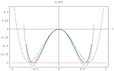
Figure 2: The effective tachyon potential in the Feynman-Siegel gauge at level $(\frac{1}{2},1)$ (dashed line), level (2,4) (dotted line) and level (2,6) (solid line). The dashed straight line indicates the expected depth of $-1$. At level (2,6) the branch ends at $t\simeq\pm 0.691$.

The minimum value calculated at level (2,6) is surprisingly close to the expected value of $-1$ times the D9-brane tension, but we consider it as just a coincidence because it is not clear at all even whether the minimum value of the potential is really converging or not.

The multiscalar tachyon potential at level $(\frac{5}{2},5)$ in the Feynman-Siegel gauge has been calculated by Raeymaekers [19]. He argued that, although there exists a candidate tachyon vacuum solution, the branch of the potential on which the candidate tachyon vacuum exists does not cross the unstable perturbative vacuum ($V_{\mathrm{eff}}(t=0)=0$), so that it should not be considered as the correct tachyon vacuum solution. In fact, when we used his multi-scalar lagrangian to calculate the effective tachyon potential starting from the perturbative vacuum, we have found that the branch connected to the perturbative vacuum hits a singularity before it reaches a minimum (see Fig.3).

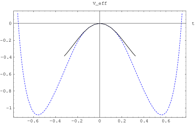
Figure 3: The effective tachyon potential in the Feynman-Siegel gauge at level $(\frac{5}{2},5)$ (solid line). The branch ends at $t\simeq\pm 0.322$. The dotted line shows the potential at level (2,4).

In view of the result [28] obtained in bosonic string field theory, it may indicate that the Feynman-Siegel gauge choice is no longer valid beyond this singularity. If this is the case, we have to find a good gauge choice which works well at level ($\frac{5}{2},5$) or higher.

$3v_{2}-3v_{4}+2v_{5}=0$ with $v_{9}=0$
In [15] Aref’eva, Belov, Koshelev and Medvedev proposed the gauge choice $3v_{2}-3v_{4}+2v_{5}=0$ such that the terms linear in $v_{6}$ should vanish, and in a subsequent paper [29] they studied the validity of this gauge in the level truncation scheme. With this choice, the equations of motion admit a solution with $v_{6}=0$, which makes the analysis much simplified. They also proposed that the string field configurations should be restricted to the space of $\phi$-charge 0 or 1. That is, if we expand the NS string field as $A=\sum_{q\in\mathbb{Z}}A_{q}$ according to $\phi$-charge $q$, then we should set $A_{q}=0$ for $q\neq 0,1$. This means that the coefficient $v_{9}$ of $b\eta\partial\eta e^{2\phi}$ is set to zero. We refer to the conditions $3v_{2}-3v_{4}+2v_{5}=0,v_{9}=0$ as ‘ABKM gauge’ below. As already claimed in [15], the solutions at levels (2,4) and (2,6) coincide with each other in this gauge, and we find

$$V^{(2,4)}\big{|}_{\mathrm{min}}=V^{(2,6)}\big{|}_{\mathrm{min}}=-1.05474\ \tilde{\tau}_{9},$$

which confirms their result.

$(b_{1}+b_{-1})A_{\pm}=0$
In a pioneering paper [10] Preitschopf, Thorn and Yost proposed a gauge choice (which we call ‘PTY gauge’)

$$(b_{1}+b_{-1})A_{\pm}(0)=\oint\frac{dz}{2\pi i}(1+z^{2})b(z)A_{\pm}(0)=0,$$ (5.10)

and showed that the correct tree-level scattering amplitudes were obtained in this gauge. We have also used this gauge to look for the non-perturbative tachyon vacuum solution. The condition (5.10) relates the coefficient of the state $c_{-1}|\psi\rangle$ to that of $c_{1}|\psi\rangle$, where $|\psi\rangle$ is an arbitrary state of ghost number 0 and picture number 0 which contains neither $c_{1}$ nor $c_{-1}$. Up to level 2, only one state $c_{-1}|0\rangle\simeq\frac{1}{2}\partial^{2}c(0)$ contains the $c_{-1}$ mode, so the gauge condition (5.10) implies

$$v_{1}=-\frac{1}{\sqrt{2}}u.$$

With this condition, however, we have not found any suitable solution for the tachyon vacuum. For example, at level (2,4) we have found a solution with vevs $u\simeq-0.446$ and $t\simeq 0.553$, but its energy density is about 203% of the expected value. At level (2,6), we have found no solution around the above point in the field configuration space. This indicates that the PTY gauge may not be useful in searching for the non-perturbative tachyon vacuum solution.

Without gauge fixing

Finally we look for the tachyon vacuum solution without any gauge-fixing conditions. From Fig. 4 one sees that, at level (2,4), the effective tachyon potential in this case shows a similar behavior to the Feynman-Siegel gauge potential (Fig. 2).

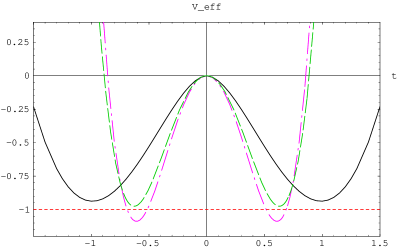
Figure 4: The gauge-unfixed effective tachyon potential at level $(\frac{1}{2},1)$ (dashed line), level (2,4) (chain line) and level (2,6) (solid line).

Its depth is about 109% of the expected D-brane tension. At the next level (2,6), however, the value of the tachyon field at the minimum becomes too large, although the potential depth $\simeq-0.937\ \tilde{\tau}_{9}$ may seem to be reasonable. Hence it is doubtful whether the effective tachyon potential without gauge-fixing really converges or not.

The results obtained in this subsection are summarized in Table 1.

level	Feynman-Siegel gauge	ABKM gauge	PTY gauge	gauge unfixed
($\frac{1}{2},1$)	$-0.974776$
(2,4)	$-1.08273$	$-1.05474$	$-2.02738$	$-1.08791$
(2,6)	$-0.999584$		—	$-0.937313$

Table 1: The depth of the tachyon potential calculated in several gauges (normalized by the non-BPS D9-brane tension).

5.2 Non-perturbative vacuum on a BPS D-brane?

Given that there exists a negative-dimensional operator $c$ in the GSO($+$) sector, one might wonder whether it induces a ‘tachyon condensation’ even in the GSO-projected theory, i.e. on a BPS D-brane. More than a decade ago, Aref’eva, Medvedev and Zubarev used modified cubic superstring field theory with the picture-changing operator $\mathcal{Z}$ (2.4) to explore such a possibility [16]. In this theory, the cubic self-interaction $u^{3}$ among the auxiliary field $u$ does not vanish, so that the effective potential for $u$ takes the ‘cubic form’ just like the tachyon potential in bosonic string field theory. Then it becomes possible for $u$ to condense to the local minimum of its potential, though to our present knowledge we cannot give any physical interpretation to such a solution. They also argued that the spacetime supersymmetry was spontaneously broken in this vacuum.

What happens if we carry out the same analysis in modified cubic superstring field theory with $Y_{-2}=Y(i)Y(-i)$, which is of our interest? The GSO-projected action can be obtained simply by setting all the GSO($-$) components to zero in the non–GSO-projected action (A.1). At level (2,4) in the Feynman-Siegel gauge, the effective potential for $u$ seems to have a minimum at $u\simeq-0.476$ (Fig. 5A).

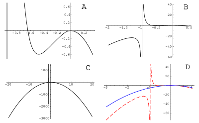
Figure 5: The Feynman-Siegel gauge effective potential for $u$ in the GSO-projected theory. A–C: The level (2,4) potential at various ranges. D: The potential at level (2,4) (dashed line) and at level (2,6) (solid line) where the singular structure has been resolved.

However, this critical point, together with the singularity at $u\simeq-0.952$, disappears in the level (2,6) potential (Fig. 5D). Furthermore, without gauge fixing, there is no extremum in the effective potential up to level (2,6) (Fig. 6).

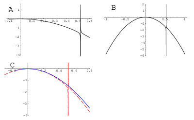
Figure 6: The gauge-unfixed effective potential for $u$ in the GSO-projected theory. A–B: The level (2,4) potential at different ranges. C: The potential at level (2,4) (dashed line) and at level (2,6) (solid line).

From these results, we conclude that there are no locally stable vacua to which the auxiliary field $u$ condenses. This is in agreement with the expectation that the BPS D-brane is stable.

5.3 A brief survey of spatially inhomogeneous condensation

An efficient method for constructing lower-dimensional D-branes as tachyon lump solutions in bosonic string field theory was invented by Moeller, Sen and Zwiebach [30], and it was shown in [31] that this method can also be applied to the case of Berkovits’ superstring field theory where a kink solution on a non-BPS D-brane represents a BPS D-brane of one lower dimension. In this method we suppose that not only the oscillator non-zero modes but also the center-of-mass momentum $e^{ikX}$ contributes to the level. For example, $ce^{ikX}$ and $\psi^{\mu}\eta e^{\phi}e^{ikX}$ have level numbers $\alpha^{\prime}k^{2}$ and $\alpha^{\prime}k^{2}+1$, respectively. The truncation of the string field at level $N$ means that we drop all terms in the string field with levels higher than $N$. Let us consider the field configurations which depend only on one spatial direction, say $x\equiv x^{9}$, and set $k_{\mu}=0$ for all $\mu\neq 9$. If we compactify the $x$-direction on a circle of radius $R$, the momentum $k\equiv k_{9}$ is discretized as $k_{n}=n/R$. As a result, the total number of degrees of freedom remains finite at any finite level even after the inclusion of the non-zero momentum modes. The computational framework based on the above procedure is called ‘modified level truncation scheme’.

Here we apply the above method to the modified cubic superstring field theory defined on a non-BPS D9-brane. By substituting

$$u(x)=u_{0}+2\sum_{n=1}^{n_{\mathrm{max}}}u_{n}\cos\frac{n}{R}x,\qquad t(x)=\sum_{r=1/2}^{r_{\mathrm{max}}}\tau_{r}\sin\frac{n}{R}x$$ (5.11)

into the action (3.22) and extremizing it with respect to $\{u_{n},\tau_{r}\}$, we can find a solution which corresponds to the BPS D8-brane at the lowest level of approximation. More details are found in [31]. We show the two sets of results: level $(\frac{4}{3},\frac{19}{6})$ for $R=\sqrt{3\alpha^{\prime}}$ and level $(\frac{67}{36},\frac{25}{6})$ for $R=3\sqrt{\alpha^{\prime}}$. From the tachyon profile $t(x)$ shown in Fig. 7, we see that the tachyon field correctly approaches one of the tachyon vacua in the asymptotic regions.

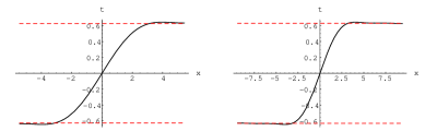
Figure 7: Kink solutions at $R=\sqrt{3\alpha^{\prime}}$ (left) and at $R=3\sqrt{\alpha^{\prime}}$ (right).

The energy density $\mathcal{T}_{8}$ of the kink solution relative to the BPS D8-brane tension $\tau_{8}$ can be calculated by the formula [31]

$$r\equiv\frac{\mathcal{T}_{8}}{\tau_{8}}=\sqrt{2}\frac{R}{\sqrt{\alpha^{\prime}}}(f(A_{\mathrm{kink}})-f(A_{0})),$$ (5.12)

where $f=-S/(2\pi RV_{9}\tilde{\tau}_{9})$, and $A_{\mathrm{kink}},A_{0}$ denote the kink solution and the tachyon vacuum solution, respectively. The expected value of $r$ is, of course, 1. We have found

$$r=1.01499 \mathrm{for} R=\sqrt{3\alpha^{\prime}},$$ (5.13)

$$r=1.01441 \mathrm{for} R=3\sqrt{\alpha^{\prime}}.$$

Although we again regard these close agreements as accidental, these results suggest that the modified cubic theory truncated to low levels captures the quantitative as well as qualitative features of the space-dependent tachyon condensation. It would also be interesting to calculate the energy distribution of the kink solution in the $x$-direction, as was done in [32] for the lump solution in bosonic string field theory.

From the definition of the modified level it is clear that the modified level truncation scheme cannot be applied to the study of time-dependent solutions, because the level number is not bounded below if we allow large time-like momenta $k^{2}<0$, by which the level truncation procedure itself is invalidated. Instead, using the oscillator-level truncation scheme (i.e. the action (3.22)) Aref’eva et al. found numerically a time-dependent solution of cubic superstring field theory equations of motion in which the tachyon starts rolling from the unstable vacuum and approaches one of the tachyon vacua in the asymptotic future [33]. On the other hand, in bosonic string theory where the tachyon potential has its minimum at a finite distance away from the origin, nobody has succeeded so far in constructing a time-dependent solution with a desirable rolling profile (see e.g. [34, 35, 36, 37]).

6 Level Truncation Analysis in Vacuum Superstring Field Theory

In bosonic VSFT, Gaiotto, Rastelli, Sen and Zwiebach showed by the level truncation analysis that there exists a spacetime-independent solution whose form, up to an overall normalization, converges to the twisted butterfly state [38]. It is believed that this solution corresponds to a spacetime-filling D25-brane. This result can be considered as a piece of evidence for the usefulness of the level truncation calculations in VSFT. Here we will try a similar analysis in vacuum superstring field theory.

6.1 Cubic vacuum superstring field theory

Following an earlier work [22], we proposed the following form of $\widehat{\mathcal{Q}}$ as a candidate kinetic operator of vacuum superstring field theory [14]:

$$\widehat{\mathcal{Q}}=\mathcal{Q}_{\mathrm{odd}}\otimes\sigma_{3}+\mathcal{Q}_{\mathrm{even}}\otimes(-i\sigma_{2});$$ (6.1)

$$\mathcal{Q}_{\mathrm{odd}}=\frac{1}{2i\varepsilon_{r}^{2}}(c(i)-c(-i))-\frac{q_{1}^{2}}{2}\oint\frac{dz}{2\pi i}b\gamma^{2}(z),$$

$$\mathcal{Q}_{\mathrm{even}}^{\mathrm{GSO}(+)}=\frac{q_{1}}{2i\varepsilon_{r}}(\gamma(i)-\gamma(-i)),$$

$$\mathcal{Q}_{\mathrm{even}}^{\mathrm{GSO}(-)}=-\frac{q_{1}}{2\varepsilon_{r}}(\gamma(i)+\gamma(-i)),$$

with $\varepsilon_{r}\to 0$ and $q_{1}$ is some unknown constant. This operator was constructed such that:

• $\widehat{\mathcal{Q}}$ should satisfy the axioms such as nilpotency, derivation property and hermiticity in order for $\widehat{\mathcal{Q}}$ to be used to construct (classically) gauge invariant actions,

• $\widehat{\mathcal{Q}}$ should have vanishing cohomology in order to support no perturbative physical open string degrees of freedom around the tachyon vacuum,

• $\widehat{\mathcal{Q}}$ should preserve the twist symmetry of the action,

• $\mathcal{Q}_{\mathrm{even}}$ should be non-zero in order that the VSFT action does not possess the $\mathbb{Z}_{2}$ GSO symmetry under $A_{-}\to-A_{-}$, because such a symmetry should be spontaneously broken after the tachyon condenses to one of the stable vacua (Fig.8).

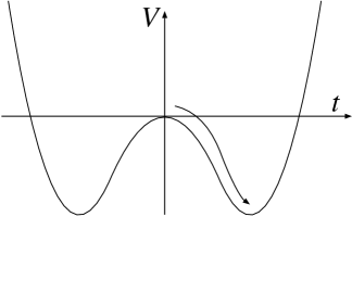
Figure 8: The reflection symmetry should be spontaneously broken after the tachyon condensation.

In spite of some efforts [39, 40, 41, 14], no exact solution representing the unstable D9-brane has been found so far.

Cubic vacuum superstring field theory action is given by

$$S_{V} = \frac{\kappa_{0}}{2}\mathrm{Tr}\left[\frac{1}{2}\langle\!\langle\widehat{Y}_{-2}|\widehat{\mathcal{A}},\widehat{\mathcal{Q}}\widehat{\mathcal{A}}\rangle\!\rangle+\frac{1}{3}\langle\!\langle\widehat{Y}_{-2}|\widehat{\mathcal{A}},\widehat{\mathcal{A}}*\widehat{\mathcal{A}}\rangle\!\rangle\right]$$

$$= \kappa_{0}\biggl{[}\frac{1}{2}\langle\!\langle Y_{-2}|\mathcal{A}_{+},\mathcal{Q}_{\mathrm{odd}}\mathcal{A}_{+}\rangle\!\rangle+\frac{1}{2}\langle\!\langle Y_{-2}|\mathcal{A}_{-},\mathcal{Q}_{\mathrm{odd}}\mathcal{A}_{-}\rangle\!\rangle+\langle\!\langle Y_{-2}|\mathcal{A}_{-},\mathcal{Q}_{\mathrm{even}}^{\mathrm{GSO}(+)}\mathcal{A}_{+}\rangle\!\rangle$$

$${}+\frac{1}{3}\langle\!\langle Y_{-2}|\mathcal{A}_{+},\mathcal{A}_{+}*\mathcal{A}_{+}\rangle\!\rangle+\langle\!\langle Y_{-2}|\mathcal{A}_{-},\mathcal{A}_{+}*\mathcal{A}_{-}\rangle\!\rangle\biggr{]},$$

where we have set $\alpha^{\prime}=1$ and $\kappa_{0}$ is some positive constant. Here, a surprising thing happens: Since $c(\pm i)$ are in the kernel of $Y(i)Y(-i)$, such terms in $\mathcal{Q}_{\mathrm{odd}}$ give no contributions to the action. On the other hand, $\gamma(\pm i)$ in $\mathcal{Q}_{\mathrm{even}}$ are still non-vanishing because

$$\lim_{z\to i}Y(z)\eta e^{\phi}(i)=-ce^{-\phi}(i)$$

is finite. One may consider it is absurd that the $c$-ghost insertions at the open string midpoint vanish, but we will proceed anyway. After the rescaling $\mathcal{A}_{\pm}\to\frac{q_{1}^{2}}{2}\mathcal{A}_{\pm}$ of the string fields, the VSFT action can be arranged as

$$S_{V} = \kappa_{0}\left(\frac{q_{1}^{2}}{2}\right)^{3}\biggl{[}\frac{1}{2}\langle\!\langle Y_{-2}|\mathcal{A}_{+},Q_{2}\mathcal{A}_{+}\rangle\!\rangle+\frac{1}{2}\langle\!\langle Y_{-2}|\mathcal{A}_{-},Q_{2}\mathcal{A}_{-}\rangle\!\rangle$$

$$\hskip 51.21504pt{}+\frac{1}{i\epsilon}\langle\!\langle Y_{-2}|\mathcal{A}_{-},(\gamma(i)-\gamma(-i))\mathcal{A}_{+}\rangle\!\rangle$$

$$\hskip 51.21504pt{}+\frac{1}{3}\langle\!\langle Y_{-2}|\mathcal{A}_{+},\mathcal{A}_{+}*\mathcal{A}_{+}\rangle\!\rangle+\langle\!\langle Y_{-2}|\mathcal{A}_{-},\mathcal{A}_{+}*\mathcal{A}_{-}\rangle\!\rangle\biggr{]},$$

where $Q_{2}\equiv-\oint\frac{dz}{2\pi i}b\gamma^{2}(z)$ and $\epsilon\equiv q_{1}\varepsilon_{r}$. Inserting the expansion

$$\mathcal{A}_{+} = \sqrt{2}uc+v_{1}\partial^{2}c+v_{2}cT^{\mathrm{m}}+v_{3}c:\partial\xi\eta:+v_{4}cT^{\phi}+v_{5}c\partial^{2}\phi$$ (6.4)

$${}+v_{6}\eta e^{\phi}G^{\mathrm{m}}+v_{7}:bc\partial c:+v_{8}\partial c\partial\phi+v_{9}b\eta\partial\eta e^{2\phi},$$

$$\mathcal{A}_{-} = t\eta e^{\phi},$$

into (6.1), we obtain the action truncated up to level (2,6). Explicit expression of it is shown in Appendix A.

Up to level (2,4), the GSO($+$) fields can be integrated out exactly. In the Siegel gauge $v_{7}=v_{8}=0$, the resulting effective potential for $t$ becomes

$$V^{(\frac{1}{2},1)}_{\mathrm{eff}}(t) \equiv -\frac{S^{(\frac{1}{2},1)}_{V,\mathrm{eff}}}{\kappa_{0}V_{10}(q_{1}^{2}/2)^{3}}=\frac{t^{2}(16+9\epsilon t)^{2}}{256\epsilon^{2}},$$ (6.5)

$$V^{(2,4)}_{\mathrm{eff}}(t) \equiv -\frac{S^{(2,4)}_{V,\mathrm{eff}}}{\kappa_{0}V_{10}(q_{1}^{2}/2)^{3}}=\frac{t^{2}(96237504+119417628\epsilon t+37335269\epsilon^{2}t^{2})}{127993536\epsilon^{2}}.$$ (6.6)

Note that the potential is no longer an even function of $t$ as a consequence of the presence of $\mathcal{Q}_{\mathrm{even}}$. From the profiles shown in Fig.9,

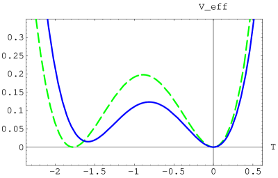
Figure 9: The cubic VSFT effective potential at level (1/2,1) (dashed line) and at level (2,4) in the Siegel gauge (solid line). The horizontal axis represents $T=\epsilon t$, while the vertical axis $\epsilon^{4}V_{\mathrm{eff}}$.

it is clear that there are two translationally invariant solutions at each level, one of which (maximum) would correspond to the unstable D9-brane, while the other (minimum) to ‘another tachyon vacuum’ with vanishing energy density. If we did not impose any gauge-fixing condition, we would obtain the effective potential shown in Fig. 10 at level (2,4).

Figure 10: The cubic VSFT effective potential without gauge fixing at level (2,4).

In this potential there is no clear distinction between the maximum and the non-trivial minimum. Hence we proceed by choosing the Siegel gauge.

At level (2,6) we can no longer analytically integrate out the massive fields. Instead of constructing the effective potential numerically, we solve the full set of equations of motion including that for $t$. In the Siegel gauge, we have found four real solutions. The field values and the potential height for each solution are shown in Table 2.

	level (2,4)		level (2,6)
	minimum	maximum	solution(1)	solution(2)	solution(3)	solution(4)
$\epsilon t$	$-1.58654$	$-0.812353$	$-1.17746$	$-1.27738$	$-0.602025$	$-2.21251$
$\epsilon^{2}u$	$-1.38402$	0.160340	0.293931	0.475872	$-0.554083$	2.04485
$\epsilon^{2}v_{1}$	$-1.02701$	$-0.486343$	$-0.483380$	$-0.309084$	0.528839	$-0.948461$
$\epsilon^{2}v_{2}$	0.177618	0.0701144	$0.207129$	0.156708	$-0.116926$	$-0.660358$
$\epsilon^{2}v_{3}$	$-0.330186$	$-0.255363$	$-0.311352$	$-0.174039$	$-0.0944988$	0.852255
$\epsilon^{2}v_{4}$	$-0.00116238$	$-0.139197$	$-0.161496$	$-0.0484503$	0.327373	0.260061
$\epsilon^{2}v_{5}$	1.23853	0.249494	0.132412	0.0669892	0.0981466	$-0.207735$
$v_{6}$	0	0	0	0	0	0
$v_{9}$	0.276184	$-0.463130$	0.220859	0.988841	$-3.10354$	$-2.24061$
$\epsilon^{4}V_{\mathrm{min}}$	0.0148204	0.123052	0.165213	0.175943	$-0.0233896$	$-0.625412$

Table 2: The vacuum expectation values of the fields and the height of the potential for the Siegel gauge solutions.

Comparing them with the level (2,4) solutions, we expect that the solution (1) would correspond to the maximum of the potential. However, it seems that there is no candidate solution for the minimum: The energy of the solution (3) is almost zero, but the vev of $t$ is unaccetably too small. Therefore, although the seemingly desirable double-well potential was obtained at low levels, this success may not continue to level (2,6) or higher.

6.2 Non-polynomial vacuum superstring field theory

We also examine the vacuum superstring field theory action based on the Berkovits’ formulation. It was argued in [42, 14] that the action around the tachyon vacuum should be given by simply replacing the kinetic operator $\widehat{Q}_{B}$ in (4.22) with $\widehat{\mathcal{Q}}$,

$$S_{V}=\frac{\kappa_{0}}{2}\sum_{M,N=0}^{\infty}\frac{(-1)^{N}}{(M+N+2)!}\left({M+N\atop N}\right)\mathrm{Tr}\biggl{\langle}\!\!\!\biggl{\langle}\left(\widehat{\mathcal{Q}}\widehat{\Phi}\right)\widehat{\Phi}^{M}\left(\widehat{\eta}_{0}\widehat{\Phi}\right)\widehat{\Phi}^{N}\biggr{\rangle}\!\!\!\biggr{\rangle}.$$ (6.7)

Let us first consider terms with $M+N\geq 1$. Since the conformal transformations of $c(\pm i)$ and $\gamma(\pm i)$ give rise to vanishing factors of $(f^{(n)\prime}_{k}(\pm i))^{h}$ with $h<0$, $\widehat{\mathcal{Q}}$ reduces to $\widehat{Q}_{2}=-\oint\frac{dz}{2\pi i}b\gamma^{2}(z)\otimes\sigma_{3}$, at least for Fock space states $\widehat{\Phi}$. Incidentally, this is reminiscent of the pregeometric action proposed in [43]. For the quadratic vertex ($M=N=0$) $f^{(2)\prime}_{k}(\pm i)$ is finite, so that the midpoint insertions can survive. From the above considerations, one sees that the $\mathbb{Z}_{2}$-symmetry breaking effect (i.e. $\mathcal{Q}_{\mathrm{even}}$) could come only from the GSO($+$)/GSO($-$) transition vertex

$$\langle\!\langle(\mathcal{Q}_{\mathrm{even}}\Phi_{+})(\eta_{0}\Phi_{-})\rangle\!\rangle.$$ (6.8)

However, the actual calculations show that all the above $\mathbb{Z}_{2}$-breaking terms vanish for level-2 string field (in the Feynman-Siegel gauge)

$$\Phi_{+} = a\ \xi\partial\xi c\partial^{2}ce^{-2\phi}+e\ \xi\eta+f\ \xi ce^{-\phi}G^{\mathrm{m}},$$

$$\Phi_{-} = t\ \xi ce^{-\phi}+k\ \xi c\partial^{2}(e^{-\phi})+l\ \xi c\partial^{2}\phi e^{-\phi}$$

$${}+m\ \xi cT^{\mathrm{m}}e^{-\phi}+n\ \xi\partial^{2}ce^{-\phi}+p\ \xi\partial\xi\eta ce^{-\phi}.$$

As a result, the effective potential for the lowest mode $t$ becomes left-right symmetric as shown in Fig. 11.

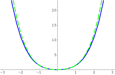
Figure 11: The non-polynomial VSFT effective potential in the Siegel gauge at levels (0,0) (dashed line) and ($\frac{3}{2},3$) (solid line).

To make matters worse, there exist no real solutions other than $\widehat{\Phi}=0$. From a lot of examples we have learned that in the successful level truncation calculations the correct (expected) qualitative behavior is reproduced already at the lowest level, and the contributions from higher-level states only give small corrections to it. If we assume this empirical law in this case as well, we should attribute the above unwelcome result to the fact that there is no $t^{3}$ term in the action at level (0,0). However, to make the 3-string vertex $\langle\!\langle(\mathcal{Q}_{\mathrm{even}}\Phi_{-})\Phi_{-}(\eta_{0}\Phi_{-})\rangle\!\rangle$ non-vanishing for $\Phi_{-}=t\xi ce^{-\phi}$ we must modify the precise form of $\mathcal{Q}_{\mathrm{even}}$. In particular, the insertion of the negative-dimensional operators to the open string midpoint does not fulfill this purpose. However, no alternatives are available now since it is very difficult to construct nilpotent $\widehat{\mathcal{Q}}$ with $\mathcal{Q}_{\mathrm{even}}\neq 0$.

7 Summary and Discussion

In the first half (sections 2–4) of this paper, we have examined the component structure of the superstring field theory action in some detail. We have explicitly shown that in modified cubic theory the correct Maxwell action (2.34) and tachyon action (3.22) are obtained after integrating out the auxiliary fields. We have specified the precise way of fixing the sign ambiguities arising in the conformal factors of the GSO($-$) components in the case of the UHP representation of the string vertices. Furthermore, we have discussed the conditions on the string fields which guarantee the reality of the action, for all of modified cubic, Witten’s cubic and Berkovits’ non-polynomial superstring field theories, using the CFT method.

The latter half is devoted to the level truncation analysis of the tachyon condensation problems. In modified cubic superstring field theory, though the tachyon potential on a non-BPS D-brane as well as its minimum is well constructed up to level (2,6) in the Feynman-Siegel gauge, its extension to higher levels may be subtle. We have not found any gauge choice which seems particularly better than the Feynman-Siegel gauge. Restricting ourselves to the lowest level ($\frac{1}{2},1$), we have obtained the static kink solution representing a BPS D-brane of one lower dimension, whose energy density is remarkably close to the expected D-brane tension ($\sim$101%). We have also verified that no such non-perturbative vacuum as was found in [16] in the theory with the picture-changing operator $\mathcal{Z}$ exists on a BPS D-brane if we employ $Y(i)Y(-i)$ as the picture-changing operator which is preferable to $\mathcal{Z}$. Lastly, we have investigated whether vacuum superstring field theory with the pure-ghost kinetic operator (6.1) can support the correct (expected) solutions in the level truncation scheme. Unfortunately, we have obtained disappointing results in both of cubic and Berkovits’ non-polynomial theories.

In the study of tachyon condensation in modified cubic superstring field theory, we have found the following unusual features: (i) The potential depth and the kink tension are very close to the expected values already at the lowest level $\left(\frac{1}{2},1\right)$, (ii) The vacuum energy does not seem to improve regularly as the truncation level is increased, (iii) The tachyon vacuum is not reached in the Feynman-Siegel gauge at level $\left(\frac{5}{2},5\right)$ [19]. These are in contrast with the results obtained in bosonic and Berkovits’ theories (see [44, 25]). We consider these behaviors should be attributed to the unconventional choice (0-picture) of field variables. More precisely, we would like to suggest the following interpretation: Let us recall that a solution $\Phi_{0}$ in Berkovits’ superstring field theory and a solution $A_{0}$ in modified cubic theory which share the same physical content are formally related through the map $A_{0}=e^{-\Phi_{0}}Q_{B}e^{\Phi_{0}}$ (see [14] for details). Then, the low-lying fields in $A_{0}$ would receive contributions from various higher modes in $\Phi_{0}$, because the $*$-product mixes fields of different levels. Furthermore, since $b_{0}$ is not a derivation of the $*$-algebra, a Siegel gauge solution $\Phi_{0}$ in Berkovits’ theory does not in general map to a Siegel gauge solution $A_{0}$ in modified cubic theory. Given that the Siegel gauge solution for the tachyon vacuum shows the ‘regular’ behavior in Berkovits’ theory [25], the above consideration may give a possible explanation for all the strange behaviors (i)–(iii) of modified cubic theory, though we cannot prove it at all.

In light of the results obtained in the level truncation analysis of vacuum superstring field theory, it seems that the pure-ghost kinetic operator (6.1) fails to describe the theory around the tachyon vacuum. It is even possible that the pure-ghost ansatz for the kinetic operator is too simple to correctly reproduce the complicated D-brane spectrum of type II superstring theory. If this is indeed true, we have to look for a matter-ghost mixed kinetic operator which is suitable for the description of the tachyon vacuum. This would require us to make a fresh start for the construction of vacuum superstring field theory.

Appendices

A Cubic Action at Level (2,6)

The cubic action truncated at level (2,6) is found to be (in units where $\alpha^{\prime}=1$)

$$f = -\frac{S}{\tilde{\tau}_{9}V_{10}}=-\frac{2\pi^{2}g_{o}^{2}S}{V_{10}}\equiv f_{\mathrm{quad}}+f_{\mathrm{cubic}};$$ (A.1)

$$f_{\mathrm{quad}} = -2\pi^{2}\biggl{[}\frac{1}{4}t^{2}+\frac{1}{2}u^{2}+\sqrt{2}uv_{1}+v_{1}^{2}+\frac{15}{8}v_{2}^{2}-\frac{1}{\sqrt{2}}uv_{3}+2v_{1}v_{3}$$ (A.2)

$${}+\frac{1}{4}v_{3}^{2}-2\sqrt{2}uv_{4}-8v_{1}v_{4}-4v_{3}v_{4}+\frac{77}{8}v_{4}^{2}+2\sqrt{2}uv_{5}+6v_{1}v_{5}+v_{3}v_{5}$$

$${}-13v_{4}v_{5}+\frac{11}{2}v_{5}^{2}-\frac{15}{2}v_{2}v_{6}+\frac{15}{2}v_{4}v_{6}-5v_{5}v_{6}+\frac{5}{2}v_{6}^{2}+\frac{1}{\sqrt{2}}uv_{7}+v_{1}v_{7}$$

$${}-\frac{1}{2}v_{3}v_{7}-2v_{4}v_{7}+2v_{5}v_{7}+3v_{3}v_{8}-5v_{4}v_{8}+2v_{5}v_{8}+v_{7}v_{8}+\frac{1}{\sqrt{2}}uv_{9}$$

$${}+2v_{1}v_{9}-\frac{15}{4}v_{2}v_{9}+v_{3}v_{9}-\frac{5}{4}v_{4}v_{9}+v_{5}v_{9}+v_{7}v_{9}+v_{8}v_{9}\biggr{]},$$

$$f_{\mathrm{cubic}} = -2\pi^{2}\bigg{[}\frac{9\sqrt{2}}{16}t^{2}u+\frac{9}{8}t^{2}v_{1}-\frac{25}{32}t^{2}v_{2}-\frac{9}{16}t^{2}v_{3}-\frac{59}{32}t^{2}v_{4}+\frac{43}{24}t^{2}v_{5}+\frac{40}{9}\sqrt{\frac{2}{3}}uv_{6}^{2}$$ (A.3)

$${}+\frac{80}{9\sqrt{3}}v_{1}v_{6}^{2}-\frac{20}{9\sqrt{3}}v_{2}v_{6}^{2}-\frac{40}{9\sqrt{3}}v_{3}v_{6}^{2}-\frac{1180}{81\sqrt{3}}v_{4}v_{6}^{2}+\frac{3440}{243\sqrt{3}}v_{5}v_{6}^{2}+\frac{2}{3}t^{2}v_{7}$$

$${}+\frac{1280}{243\sqrt{3}}v_{6}^{2}v_{7}+\sqrt{3}u^{2}v_{9}+\frac{70}{9}\sqrt{\frac{2}{3}}uv_{1}v_{9}+\frac{86}{9\sqrt{3}}v_{1}^{2}v_{9}-\frac{25}{3\sqrt{6}}uv_{2}v_{9}-\frac{875}{81\sqrt{3}}v_{1}v_{2}v_{9}$$

$${}+\frac{4435}{648\sqrt{3}}v_{2}^{2}v_{9}+\frac{5}{9}\sqrt{\frac{2}{3}}uv_{3}v_{9}+\frac{350}{243\sqrt{3}}v_{1}v_{3}v_{9}-\frac{125}{162\sqrt{3}}v_{2}v_{3}v_{9}-\frac{37}{18\sqrt{3}}v_{3}^{2}v_{9}$$

$${}-\frac{193}{9\sqrt{6}}uv_{4}v_{9}-\frac{6755}{243\sqrt{3}}v_{1}v_{4}v_{9}+\frac{4825}{324\sqrt{3}}v_{2}v_{4}v_{9}-\frac{965}{486\sqrt{3}}v_{3}v_{4}v_{9}+\frac{39809}{1944\sqrt{3}}v_{4}^{2}v_{9}$$

$${}+\frac{86}{9}\sqrt{\frac{2}{3}}uv_{5}v_{9}+\frac{6020}{243\sqrt{3}}v_{1}v_{5}v_{9}-\frac{1075}{81\sqrt{3}}v_{2}v_{5}v_{9}+\frac{430}{243\sqrt{3}}v_{3}v_{5}v_{9}-\frac{979}{27\sqrt{3}}v_{4}v_{5}v_{9}$$

$${}+\frac{4082}{243\sqrt{3}}v_{5}^{2}v_{9}+\frac{8}{3}\sqrt{\frac{2}{3}}uv_{7}v_{9}+\frac{1552}{243\sqrt{3}}v_{1}v_{7}v_{9}-\frac{100}{27\sqrt{3}}v_{2}v_{7}v_{9}+\frac{40}{81\sqrt{3}}v_{3}v_{7}v_{9}$$

$${}-\frac{772}{81\sqrt{3}}v_{4}v_{7}v_{9}+\frac{688}{81\sqrt{3}}v_{5}v_{7}v_{9}+\frac{16}{9}\sqrt{\frac{2}{3}}uv_{8}v_{9}+\frac{32}{9\sqrt{3}}v_{1}v_{8}v_{9}-\frac{200}{81\sqrt{3}}v_{2}v_{8}v_{9}$$

$${}+\frac{80}{243\sqrt{3}}v_{3}v_{8}v_{9}-\frac{1544}{243\sqrt{3}}v_{4}v_{8}v_{9}+\frac{1120}{243\sqrt{3}}v_{5}v_{8}v_{9}+\frac{256}{81\sqrt{3}}v_{7}v_{8}v_{9}\biggr{]}.$$

As a verification of our result, let us compare it with the results of refs. [19, 15]. Our function $f$ (A.1) up to level (2,4) precisely agrees with that of Raeymaekers [19], if we make the replacements

$$v_{7}\to 0,\quad v_{8}\to 0,\quad(\mbox{Feynman-Siegel gauge})$$ (A.4)

$$v_{6}\to-v_{6},\quad u\to\frac{u}{\sqrt{2}},\quad t\to\frac{t}{2},$$

and then $v_{9}\to v_{7}$. Ours, however, does not coincide with the result of Aref’eva et al. (version 3 of [15]) even after setting

$$v_{6}\to-v_{6},\quad v_{9}\to 0,\quad u\to\frac{u}{\sqrt{2}},\quad t\to\frac{t}{2}.$$ (A.5)

In view of our and Raeymaeker’s results, the $-$ sign in front of the parenthesis in the last line of eq.(3.3) of (version 3 of) [15] should be $+$. If so, ours and theirs agree with each other.

The cubic vacuum superstring field theory action truncated up to level (2,6) is, after the rescaling $\mathcal{A}_{\pm}\to(q_{1}^{2}/2)\mathcal{A}_{\pm}$ mentioned in subsection 6.1, given by

$$S_{V} = \kappa_{0}\left(\frac{q_{1}^{2}}{2}\right)^{3}V_{10}\left(-\tilde{f}_{\mathrm{quad}}-\frac{1}{2\pi^{2}}f_{\mathrm{cubic}}\right),$$ (A.6)

$$-\tilde{f}_{\mathrm{quad}} = \frac{1}{2}u^{2}+\sqrt{2}uv_{1}+v_{1}^{2}+\frac{15}{8}v_{2}^{2}-\frac{1}{\sqrt{2}}uv_{3}+2v_{1}v_{3}+\frac{1}{4}v_{3}^{2}-2\sqrt{2}uv_{4}-8v_{1}v_{4}$$

$${}-4v_{3}v_{4}+\frac{77}{8}v_{4}^{2}+2\sqrt{2}uv_{5}+6v_{1}v_{5}+v_{3}v_{5}-13v_{4}v_{5}+\frac{11}{2}v_{5}^{2}+\frac{1}{\sqrt{2}}uv_{7}$$

$${}+v_{1}v_{7}-\frac{1}{2}v_{3}v_{7}-2v_{4}v_{7}+2v_{5}v_{7}+3v_{3}v_{8}-5v_{4}v_{8}+2v_{5}v_{8}+v_{7}v_{8}$$

$${}+\frac{1}{\epsilon}\left(\sqrt{2}tu+2tv_{1}-tv_{3}-\frac{5}{2}tv_{4}+3tv_{5}+tv_{7}\right),$$

where $\epsilon=q_{1}\varepsilon_{r}$ and $f_{\mathrm{cubic}}$ is the same as in (A.3).

B Technical Remarks about the Correlators and the Conformal Transform of $e^{ikX}$

The fact that each $X^{\mu}$ contains both left- and right-movers makes the computations of the correlators including $X^{\mu}$ in the open string case complicated. In the presence of the open string boundary, the OPE between two $X$’s inserted in the interior of the world-sheet becomes [45]

$$X^{\mu}(z,\bar{z})X^{\nu}(w,\bar{w})\sim-\frac{\alpha^{\prime}}{2}\eta^{\mu\nu}\ln|z-w|^{2}-\frac{\alpha^{\prime}}{2}\eta^{\mu\nu}\ln|z-\bar{w}|^{2}.$$ (B.1)

Hence, when two $X$’s are inserted on the boundary ($z=\bar{z},w=\bar{w}$) we should have

$$X^{\mu}(z)X^{\nu}(w)\sim-2\alpha^{\prime}\eta^{\mu\nu}\ln(z-w),$$ (B.2)

where $z,w$ are real numbers satisfying $z>w$. The $XX$ OPE appearing in (2.20) should be understood this way.

If we want to calculate the string field theory vertices for string fields having non-zero momenta, we must compute the conformal transformations $f^{(n)}_{k}\circ e^{ikX}$ and the correlators $\langle e^{ik_{1}X(z_{1})}\cdots e^{ik_{n}X(z_{n})}\rangle_{\mathrm{UHP}}$. Since the world-sheet scalars $X^{\mu}$ are bosonic variables, two exponentials of $X$ must commute with each other without any phase factor irrespective of the values of momenta. For the OPE to be consistent with this commutation rule, we must have

$$:e^{ik_{1}X(z_{1})}::e^{ik_{2}X(z_{2})}:\ \sim|z_{1}-z_{2}|^{2\alpha^{\prime}k_{1}\cdot k_{2}}:e^{ik_{1}X(z_{1})+ik_{2}X(z_{2})}:,$$ (B.3)

$$\partial X^{\mu}(z):e^{ikX(w)}:\ =\ :e^{ikX(w)}:\partial X^{\mu}(z)\sim-\frac{2\alpha^{\prime}ik^{\mu}}{z-w}:e^{ikX(w)}:,$$

on the boundary. In general, the $n$-point correlator among $e^{ik_{j}X(z_{j})}$ becomes

$$\langle e^{ik_{1}X(z_{1})}\cdots e^{ik_{n}X(z_{n})}\rangle_{\mathrm{UHP}}=\left(\prod_{i>j}|z_{i}-z_{j}|^{2\alpha^{\prime}k_{i}\cdot k_{j}}\right)(2\pi)^{10}\delta^{10}\left(\sum k_{i}\right).$$ (B.4)

From the remark in the last paragraph, it would be natural to consider that the conformal factor of $e^{ikX}$ contains both contributions from holomorphic and antiholomorphic sides. Then, since $e^{ikX}$ is a primary field of conformal weight $\alpha^{\prime}k^{2}$, the conformal transform of $e^{ikX}$ by $f$ should be given by

$$f\circ e^{ikX(z)}=|f^{\prime}(z)|^{\alpha^{\prime}k^{2}}e^{ikX(f(z))}.$$ (B.5)

Otherwise, the phase of the conformal factor would be ill-defined for a general value of momentum. In the particular case of $f=I$ (inversion), we have

$$I\circ e^{ikX(z)}=|z^{-2}|^{\alpha^{\prime}k^{2}}e^{ikX(-1/z)}.$$ (B.6)

Finally, the hermitian conjugation of $e^{ikX(z)}$ is defined to be

$$\left(e^{ikX(z)}\right)^{\dagger}=|z^{-2}|^{\alpha^{\prime}k^{2}}e^{-ikX(1/z^{*})},$$ (B.7)

in accordance with (B.6). Note that there is no difference between $z^{2}$ and $|z^{2}|$ for real $z$. We have performed all the calculations in the text according to the above rules.

References

• [1] D. Friedan, E. Martinec and S. Shenker, “Conformal Invariance, Supersymmetry and String Theory,” Nucl. Phys. B271 (1986) 93.
• [2] E. Witten, “Interacting Field Theory of Open Superstrings,” Nucl. Phys. B276 (1986) 291.
• [3] E. Witten, “Non-commutative Geometry and String Field Theory,” Nucl. Phys. B268 (1986) 253.
• [4] C. Wendt, “Scattering Amplitudes and Contact Interactions in Witten’s Superstring Field Theory,” Nucl. Phys. B314 (1989) 209.
• [5] N. Berkovits, “Super-Poincaré Invariant Superstring Field Theory,” Nucl. Phys. B459(1996)439 [hep-th/9503099].
• [6] N. Berkovits, “The Ramond Sector of Open Superstring Field Theory,” hep-th/0109100.
• [7] L. Barosi and C. Tello, “GSO($-$) Vertex Operators and Open Superstring Field Theory in Hybrid Variables,” hep-th/0303246.
• [8] I.Y. Aref’eva, P.B. Medvedev and A P. Zubarev, “Background Formalism for Superstring Field Theory,” Phys. Lett. 240B (1990) 356.
• [9] I.Y. Aref’eva, P.B. Medvedev and A.P. Zubarev, “New Representation for String Field Solves the Consistency Problem for Open Superstring Field Theory,” Nucl, Phys. B341 (1990) 464.
• [10] C.R. Preitschopf, C.B. Thorn and S.A. Yost, “Superstring Field Theory,” Nucl. Phys. B337 (1990) 363.
• [11] I. Bars, Phys. Lett. B517 (2001) 436-444 [hep-th/0106157];
I. Bars and Y. Matsuo, Phys. Rev. D65 (2002) 126006 [hep-th/0202030];
I. Bars and Y. Matsuo, Phys. Rev. D66 (2002) 066003 [hep-th/0204260];
I. Bars, I. Kishimoto and Y. Matsuo, Phys. Rev. D67 (2003) 066002 [hep-th/0211131];
I. Bars, hep-th/0211238;
I. Bars, I. Kishimoto and Y. Matsuo, hep-th/0302151;
I. Bars, I. Kishimoto and Y. Matsuo, hep-th/0304005.
• [12] N. Berkovits, “Review of Open Superstring Field Theory,” hep-th/0105230.
• [13] K. Bardakci, “Dual Models and Spontaneous Symmetry Breaking,” Nucl. Phys. B68 (1974) 331;
K. Bardakci and M. B. Halpern, “Explicit Spontaneous Breakdown in a Dual Model,” Phys. Rev. D10 (1974) 4230;
K. Bardakci and M. B. Halpern, “Explicit Spontaneous Breakdown in a Dual Model II: N Point Functions,” Nucl. Phys. B96 (1975) 285;
K. Bardakci, “Spontaneous Symmetry Breakdown in the Standard Dual String Model,” Nucl. Phys. B133 (1978) 297.
• [14] K. Ohmori, “On Ghost Structure of Vacuum Superstring Field Theory,” Nucl. Phys. B648 (2003) 94-130 [hep-th/0208009].
• [15] I.Y. Aref’eva, D.M. Belov, A.S. Koshelev and P.B. Medvedev, “Tachyon Condensation in Cubic Superstring Field Theory,” Nucl. Phys. B638 (2002) 3-20 [hep-th/0011117].
• [16] I.Y. Aref’eva, P.B. Medvedev and A.P. Zubarev, “Non-Perturbative Vacuum for Superstring Field Theory and Supersymmetry Breaking,” Mod. Phys. Lett. A6 (1991) 949.
• [17] B.V. Urosevic and A.P. Zubarev, “On the component analysis of modified superstring field theory actions,” Phys. Lett. 246B (1990) 391.
• [18] I.Y. Aref’eva, D.M. Belov, A.A. Giryavets, A.S. Koshelev and P.B. Medvedev, “Noncommutative Field Theories and (Super)String Field Theories,” hep-th/0111208.
• [19] J. Raeymaekers, “Tachyon condensation in string field theory: the tachyon potential in the conformal field theory approach,” Ph.D thesis, KULeuven, 2001.
• [20] N. Berkovits, “The Tachyon Potential in Open Neveu-Schwarz String Field Theory,” JHEP 0004 (2000) 022 [hep-th/0001084].
• [21] N. Berkovits, A. Sen and B. Zwiebach, “Tachyon Condensation in Superstring Field Theory,” Nucl. Phys. B587 (2000) 147-178, [hep-th/0002211].
• [22] I.Y. Aref’eva, D.M. Belov and A.A. Giryavets, “Construction of the Vacuum String Field Theory on a non-BPS Brane,” JHEP 0209 (2002) 050 [hep-th/0201197].
• [23] P.-J. De Smet and J. Raeymaekers, “The Tachyon Potential in Witten’s Superstring Field Theory,” JHEP 0008 (2000) 020 [hep-th/0004112].
• [24] K. Ohmori, “A Review on Tachyon Condensation in Open String Field Theories,” hep-th/0102085.
• [25] P.-J. De Smet, “Tachyon Condensation: Calculations in String Field Theory,” hep-th/0109182.
• [26] A. Sen, “Universality of the Tachyon Potential,” JHEP 9912(1999)027 [hep-th/9911116].
• [27] A. Sen and B. Zwiebach, “Tachyon Condensation in String Field Theory,” JHEP 0003 (2000) 002 [hep-th/9912249].
• [28] I. Ellwood and W. Taylor, “Gauge Invariance and Tachyon Condensation in Open String Field Theory,” hep-th/0105156.
• [29] I.Y. Aref’eva, D.M. Belov, A.S. Koshelev and P.B. Medvedev, “Gauge Invariance and Tachyon Condensation in Cubic Superstring Field Theory,” Nucl. Phys. B638 (2002) 21-40 [hep-th/0107197].
• [30] N. Moeller, A. Sen and B. Zwiebach, “D-branes as Tachyon Lumps in String Field Theory,” JHEP 0008 (2000) 039 [hep-th/0005036].
• [31] K. Ohmori, “Tachyonic Kink and Lump-like Solutions in Superstring Field Theory,” JHEP 0105(2001)035 [hep-th/0104230].
• [32] H. Yang, “Stress Tensors in p-adic String Theory and Truncated OSFT,” JHEP 0211 (2002) 007 [hep-th/0209197].
• [33] I.Y. Aref’eva, L.V. Joukovskaya and A.S. Koshelev, “Time Evolution in Superstring Field Theory on non-BPS brane.I. Rolling Tachyon and Energy-Momentum Conservation,” hep-th/0301137;
Y. Volovich, “Numerical Study of Nonlinear Equations with Infinite Number of Derivatives,” math-ph/0301028.
• [34] N. Moeller and B. Zwiebach, “Dynamics with Infinitely Many Time Derivatives and Rolling Tachyons,” JHEP 0210 (2002) 034 [hep-th/0207107].
• [35] J. Klusoň, “Time Dependent Solution in Open Bosonic String Field Theory,” hep-th/0208028.
• [36] M. Fujita and H. Hata, “Time Dependent Solution in Cubic String Field Theory,” hep-th/0304163.
• [37] N. Moeller and M. Schnabl, “Tachyon condensation in open-closed p-adic string theory,” hep-th/0304213.
• [38] D. Gaiotto, L. Rastelli, A. Sen and B. Zwiebach, “Ghost Structure and Closed Strings in Vacuum String Field Theory,” hep-th/0111129.
• [39] I.Y. Aref’eva, A.A. Giryavets and A.S. Koshelev, “NS Ghost Slivers,” Phys. Lett. B536 (2002) 138-146 [hep-th/0203227];
A. Koshelev, “Solutions of Vacuum Superstring Field Theory,” hep-th/0212055.
• [40] K. Ohmori, “Comments on Solutions of Vacuum Superstring Field Theory,” JHEP 0204 (2002) 059 [hep-th/0204138].
• [41] O. Lechtenfeld, A.D. Popov and S. Uhlmann, “Exact Solutions of Berkovits’ String Field Theory,” Nucl. Phys. B637 (2002) 119-142 [hep-th/0204155];
A. Kling, O. Lechtenfeld, A.D. Popov and S. Uhlmann, “On Nonperturbative Solutions of Superstring Field Theory,” Phys. Lett. B551 (2003) 193-201 [hep-th/0209186].;
A. Kling, O. Lechtenfeld, A.D. Popov and S. Uhlmann, “Solving String Field Equations: New Uses for Old Tools,” hep-th/0212335.
• [42] J. Klusoň, “Some Remarks About Berkovits’ Superstring Field Theory,” JHEP 0106 (2001) 045 [hep-th/0105319];
M. Mariño and R. Schiappa, “Towards Vacuum Superstring Field Theory: The Supersliver,” hep-th/0112231.
• [43] J. Klusoň, “Proposal for Background Independent Berkovits’ Superstring Field Theory,” JHEP 0107 (2001) 039 [hep-th/0106107];
M. Sakaguchi, “Pregeometrical Formulation of Berkovits’ Open RNS Superstring Field Theories,” hep-th/0112135.
• [44] D. Gaiotto and L. Rastelli, “Experimental String Field Theory,” hep-th/0211012.
• [45] J. Polchinski, “String Theory,” vol.1, Cambridge University Press.