Light-front Schwinger Model at Finite Temperature

Abstract

We study the light-front Schwinger model at finite temperature following the recent proposal in alves . We show that the calculations are carried out efficiently by working with the full propagator for the fermion, which also avoids subtleties that arise with light-front regularizations. We demonstrate this with the calculation of the zero temperature anomaly. We show that temperature dependent corrections to the anomaly vanish, consistent with the results from the calculations in the conventional quantization. The gauge self-energy is seen to have the expected non-analytic behavior at finite temperature, but does not quite coincide with the conventional results. However, the two structures are exactly the same on-shell. We show that temperature does not modify the bound state equations and that the fermion condensate has the same behavior at finite temperature as that obtained in the conventional quantization.

I Introduction

In an earlier paper alves , it was shown that light-front field theories brodsky do not admit a naive generalization to finite temperature. A proper thermal description of such theories was proposed in ref alves , the meaning of which was clarified nicely by Weldon weldon . The calculations carried out in refs alves ; weldon1 showed that the thermal contributions to the self-energy in scalar theories (both in $\phi^{4}$ and $\phi^{3}$ theories) at one loop coincide with the result from a conventional calculations. In this paper, we extend such an investigation to fermionic and gauge theories. In particular, we study various questions of interest within the context of the Schwinger model schwinger at finite temperature.

As is well known, the Schwinger model which describes massless QED in $1+1$ dimensions is exactly soluble and has been widely studied in both conventional klaiber ; elcio as well as light-front quantization harindranath at zero temperature. In this paper, we study various questions associated with the Schwinger model in the light-front quantization at finite temperature kapusta ; lebellac ; das . In section II, we briefly recapitulate the finite temperature formalism proposed in alves for light-front quantized theories. We give explicitly the forms of the scalar as well as the gauge boson propagators in various gauges, both in the imaginary time as well as the real time formalisms. The fermion case needs to be discussed carefully and we do this separately in section III, where we give the propagators in both the imaginary time and real time formalisms. In section IV, we undertake a detailed study of the light-front Schwinger model at finite temperature. While conventionally, in the light-front quantized theories one works with only the independent fermion components, we argue that working with the full theory can be simpler and one can even avoid subtleties generally arising from light-front regularizations. We show this by explicitly calculating the anomaly at zero temperature. We then show that the finite temperature correction to the anomaly vanishes, as is also the case in the conventional quantization karev ; das . In the case of the light-front Schwinger model, only one of the fermion components thermalizes and, consequently, we show that while the thermal self-energy for the photon has the expected non-analytic structure weldon2 ; bedaque ; hott , it does not quite agree with the conventional result adilson . However, these thermal contributions vanish on-shell in both the quantizations, once again showing equivalence in the observable sector. We also show that the bound state equation harindranath remains unchanged at finite temperature. We calculate the fermion condensate at finite temperature jayawardene ; smilga using the method of bosonization liguori and show that the result in the light-front formalism coincides with that obtained using conventional quantization. Finally, we conclude with a brief summary in section V.

II Formalism

In this section, we will briefly recapitulate the essential results from refs alves ; weldon and list the forms of the propagators for scalar and gauge fields in the light-front quantization at finite temperature. As was shown by Weldon weldon , the proposal in alves corresponds to choosing a coordinate system

$$x^{\mu}\rightarrow\bar{x}^{\mu},\qquad\mu=0,1,\cdots,n-1,$$ (1)

such that

$$\bar{x}^{0} = x^{0}+x^{n-1},$$

$$\bar{x}^{i} = x^{i},\qquad i=1,2,\cdots,n-1.$$ (2)

Such a coordinate redefinition, which does not correspond to a Lorentz transformation, has a unit Jacobian. One can quantize the theory on the light-front, $\bar{x}^{0}=0$, and in this coordinate system can preserve all the simple relations of conventional light-front quantization as well as have a thermal description of the system with a heat bath at rest.

Such a coordinate system, however, has a nontrivial metric structure in the ($2\times 2$) space of “$0$-$(n-1)$” indices, namely,

$$\bar{g}^{\mu\nu}=\left(\begin{array}[]{rr}0&-1\\ -1&-1\end{array}\right),\qquad\bar{g}_{\mu\nu}=\left(\begin{array}[]{rr}1&-1\\ -1&0\end{array}\right).$$ (3)

Furthermore, the energy-momentum, in the new coordinates, take the form

$$\bar{p}_{0} = p_{0},$$

$$\bar{p}_{n-1} = -p_{0}+p_{n-1},$$

$$\bar{p}_{\alpha} = p_{\alpha},\qquad\alpha=1,2,\cdots,n-2,$$ (4)

so that with (3), the form of the Einstein relation for a massive particle follows to be

$$(2\bar{p}_{0}+\bar{p}_{n-1})\bar{p}_{n-1}+\bar{p}_{\alpha}\bar{p}_{\alpha}+m^{2} = 0$$

$${\rm or,}\quad 2\bar{p}_{0}\bar{p}_{n-1}+\omega_{\bar{p}}^{2} = 0,$$ (5)

where we have defined

$$\omega_{\bar{p}}^{2}=\bar{p}_{i}\bar{p}_{i}+m^{2},\qquad i=1,2,\cdots,n-1.$$ (6)

In this case, the density matrix for a system, interacting with a heat bath at rest, takes the form

$$\rho(\beta)=e^{-\beta\bar{p}_{0}},$$ (7)

where $\beta=\frac{1}{T}$ in units of the Boltzmann constant. (We note parenthetically that $\bar{p}_{0}=p_{0}=\frac{1}{\sqrt{2}}(p^{+}+p^{-})$, which is what was used in alves .) The statistical description of quantum field theories can now be developed in the standard manner kapusta ; lebellac ; das . For example, we list below the propagators for bosonic (scalar and gauge) fields in both imaginary and real time (closed time path) formalisms. The propagators for the fermions would be discussed separately in the next section.

II.1 Scalar Propagator

At zero temperature, the propagator for a scalar field has the form

$$iG(\bar{p})=\frac{i}{-(2\bar{p}_{0}\bar{p}_{n-1}+\omega_{\bar{p}}^{2})+i\epsilon}.$$ (8)

The form of the propagator, in the imaginary time formalism, now follows from (8) to be

$$G^{(\beta)}(\bar{p})=\frac{1}{2\bar{p}_{0}\bar{p}_{n-1}+\omega_{\bar{p}}^{2}},$$ (9)

with $\bar{p}_{0}=\frac{2i\pi n}{\beta}$ where $n$ takes integer values.

In the real time formalism, on the other hand, the degrees of freedom are known to double das . Here, we note only the form of the propagator in the closed time path formalism (a similar form can be derived in a straightforward manner for thermofield dynamics).

$$iG_{++}(\bar{p}) = \frac{i}{-(2\bar{p}_{0}\bar{p}_{n-1}+\omega_{\bar{p}}^{2})+i\epsilon}+2\pi n_{B}(|\bar{p}_{0}|)\delta(2\bar{p}_{0}\bar{p}_{n-1}+\omega_{\bar{p}}^{2}),$$

$$iG_{+-}(\bar{p}) = 2\pi[\theta(-\bar{p}_{0})+n_{B}(|\bar{p}_{0}|)]\delta(2\bar{p}_{0}\bar{p}_{n-1}+\omega_{\bar{p}}^{2}),$$

$$iG_{-+}(\bar{p}) = 2\pi[\theta(\bar{p}_{0})+n_{B}(|\bar{p}_{0}|)]\delta(2\bar{p}_{0}\bar{p}_{n-1}+\omega_{\bar{p}}^{2}),$$

$$iG_{--}(\bar{p}) = \frac{i}{(2\bar{p}_{0}\bar{p}_{n-1}+\omega_{\bar{p}}^{2})+i\epsilon}+2\pi n_{B}(|\bar{p}_{0}|)\delta(2\bar{p}_{0}\bar{p}_{n-1}+\omega_{\bar{p}}^{2}).$$ (10)

Here,

$$n_{B}(|\bar{p}_{0}|)=\frac{1}{e^{\beta|\bar{p}_{0}|}-1},$$ (11)

represents the bosonic distribution function.

II.2 Gauge Boson Propagator

The propagators for the gauge fields can also be derived in a straightforward manner. Without going into details, let us simply note here that in the path integral formalism with a general covariant gauge, the zero temperature propagator has the form

$$iD_{\mu\nu}(\bar{p})=-\frac{i}{\bar{p}^{2}}\left(\bar{g}_{\mu\nu}-(1-\xi)\frac{\bar{p}_{\mu}\bar{p}_{\nu}}{\bar{p}^{2}}\right),$$ (12)

where $\xi$ represents the gauge fixing parameter (the Feynman prescription is understood) and

$$\bar{p}^{2}=-2\bar{p}_{0}\bar{p}_{n-1}-\bar{p}_{i}\bar{p}_{i}.$$ (13)

The finite temperature propagator, in the imaginary time formalism, has the form

$$D_{\mu\nu}^{(\beta)}(\bar{p})=\frac{1}{\bar{p}^{2}}\left(\bar{g}^{(E)}_{\mu\nu}-(1-\xi)\frac{\bar{p}_{\mu}\bar{p}_{\nu}}{\bar{p}^{2}}\right),$$ (14)

with $\bar{p}_{0}=\frac{2i\pi n}{\beta}$ and $\bar{g}^{(E)}_{\mu\nu}$ is the properly rotated Euclidean metric.

Parenthetically, we note that, as has been already pointed out in weldon , going to oblique coordinates and rotating to imaginary time do not commute. Nonetheless, once we are in the oblique coordinates, we can go to the imaginary time formalism and our conventions for this are as follows.

$$\bar{x}^{\mu}=(-i\bar{x}^{0}_{(E)},\bar{x}^{i}_{(E)}).$$ (15)

The energy-momentum vector, on the other hand, is rotated as

$$\bar{p}_{\mu}=(i\bar{p}_{0}^{(E)},\bar{p}_{i}),$$ (16)

which is required from the analytic structure of the propagator (so that we do not cross a singularity). Under the rotation in (15), it is easy to check that the component of the metric (in the $0-(n-1)$ space) transforms as (the other components of the metric do not change)

$$\bar{g}^{\mu\nu(E)}=\left(\begin{array}[]{rr}0&-i\\ -i&-1\end{array}\right),\qquad\bar{g}^{(E)}_{\mu\nu}=\left(\begin{array}[]{rr}-1&i\\ i&0\end{array}\right).$$ (17)

We note that, in an oblique coordinate system, the upper and lower index tensors can be different, which is reflected in (17). Transformation of other vectors and tensors can be determined from the rotation in (15).

In the real time formalism, the degrees of freedom will double and the propagator will have the form (once again, the Feynman prescription is understood as in (10))

$$iD_{\mu\nu,++}^{(\beta)}(\bar{p}) = -\left(\bar{g}_{\mu\nu}-(1-\xi)\frac{\bar{p}_{\mu}\bar{p}_{\nu}}{\bar{p}^{2}}\right)\left(\frac{i}{\bar{p}^{2}}+2\pi n_{B}(|\bar{p}_{0}|)\delta(\bar{p}^{2})\right),$$

$$iD_{\mu\nu,+-}^{(\beta)}(\bar{p}) = -\left(\bar{g}_{\mu\nu}-(1-\xi)\frac{\bar{p}_{\mu}\bar{p}_{\nu}}{\bar{p}^{2}}\right)2\pi\left(\theta(-\bar{p}_{0})+n_{B}(|\bar{p}_{0}|)\right)\delta(\bar{p}^{2}),$$

$$iD_{\mu\nu,-+}^{(\beta)}(\bar{p}) = -\left(\bar{g}_{\mu\nu}-(1-\xi)\frac{\bar{p}_{\mu}\bar{p}_{\nu}}{\bar{p}^{2}}\right)2\pi\left(\theta(\bar{p}_{0})+n_{B}(|\bar{p}_{0}|)\right)\delta(\bar{p}^{2}),$$

$$iD_{\mu\nu,--}^{(\beta)}(\bar{p}) = -\left(\bar{g}_{\mu\nu}-(1-\xi)\frac{\bar{p}_{\mu}\bar{p}_{\nu}}{\bar{p}^{2}}\right)\left(-\frac{i}{\bar{p}^{2}}+2\pi n_{B}(|\bar{p}_{0}|)\delta(\bar{p}^{2})\right).$$ (18)

On the other hand, in a general axial gauge, the zero temperature propagator in the path integral formalism takes the form

$$iD_{\mu\nu}(\bar{p})=-\frac{i}{\bar{p}^{2}}\left(\bar{g}_{\mu\nu}-\frac{\bar{n}_{\mu}\bar{p}_{\nu}+\bar{n}_{\nu}\bar{p}_{\mu}}{\bar{n}\cdot\bar{p}}+\frac{\bar{n}^{2}\bar{p}_{\mu}\bar{p}_{\nu}}{(\bar{n}\cdot\bar{p})^{2}}+\frac{\xi\bar{p}^{2}\bar{p}_{\mu}\bar{p}_{\nu}}{(\bar{n}\cdot\bar{p})^{2}}\right),$$ (19)

where $\bar{n}^{\mu}$ represents an arbitrary vector (not necessarily normalized). The finite temperature propagator, in this case, in the imaginary time formalism takes the form

$$D_{\mu\nu}^{(\beta)}(\bar{p})=\frac{1}{\bar{p}^{2}}\left(\bar{g}^{(E)}_{\mu\nu}-\frac{\bar{n}_{\mu}\bar{p}_{\nu}+\bar{n}_{\nu}\bar{p}_{\mu}}{\bar{n}\cdot\bar{p}}+\frac{\bar{n}^{2}\bar{p}_{\mu}\bar{p}_{\nu}}{(\bar{n}\cdot\bar{p})^{2}}+\frac{\xi\bar{p}^{2}\bar{p}_{\mu}\bar{p}_{\nu}}{(\bar{n}\cdot\bar{p})^{2}}\right),$$ (20)

with $\bar{p}_{0}=\frac{2i\pi n}{\beta}$ and $n_{\mu}$ representing the appropriately rotated Euclidean vectors. In the real time formalism, the degrees double and we simply note here the $(++)$ component of the propagator (the other components can be determined much like the forms given above)

$$iD_{\mu\nu,++}^{(\beta)}(\bar{p})=-\left(\bar{g}_{\mu\nu}-\frac{\bar{n}_{\mu}\bar{p}_{\nu}+\bar{n}_{\nu}\bar{p}_{\mu}}{\bar{n}\cdot\bar{p}}+\frac{\bar{n}^{2}\bar{p}_{\mu}\bar{p}_{\nu}}{(\bar{n}\cdot\bar{p})^{2}}+\frac{\xi\bar{p}^{2}\bar{p}_{\mu}\bar{p}_{\nu}}{(\bar{n}\cdot\bar{p})^{2}}\right)\left(\frac{i}{\bar{p}^{2}}+2\pi n_{B}(|\bar{p}_{0}|)\delta(\bar{p}^{2})\right).$$ (21)

The gauge propagators in other gauges can, of course, be easily derived, but these are the two most commonly used gauges in light-front field theories, which is why we have listed their forms.

III Fermions

In the light-front theories, the handling of the fermions is a little tricky. This is because one of the components of the fermion field becomes constrained. To see this, let us note that, under the coordinate redefinition in (2), the Dirac gamma matrices transform as

$$\bar{\gamma}^{0} = \gamma^{0}+\gamma^{n-1},$$

$$\bar{\gamma}^{i} = \gamma^{i},\qquad i=1,2,\cdots,n-1.$$ (22)

The transformed Dirac matrices satisfy the algebra

$$\left\{\bar{\gamma}^{\mu},\bar{\gamma}^{\nu}\right\}=2\bar{g}^{\mu\nu}.$$ (23)

This implies, in particular, from (3) that

$$(\bar{\gamma}^{0})^{2}=0,\quad(\bar{\gamma}^{n-1})^{2} = -1,$$

$$\bar{\gamma}^{0}\bar{\gamma}^{n-1}+\bar{\gamma}^{n-1}\bar{\gamma}^{0} = -2.$$ (24)

With these matrices, we can define the projection operators

$$P^{+}=-\frac{1}{2}\bar{\gamma}^{n-1}\bar{\gamma}^{0},\quad P^{-}=-\frac{1}{2}\bar{\gamma}^{0}\bar{\gamma}^{n-1},\quad(P^{\pm})^{\dagger}=P^{\pm},\quad P^{+}+P^{-}=1,$$ (25)

which allows us to decompose the fermion field as

$$\psi_{\pm}=P^{\pm}\psi.$$ (26)

In terms of these components, the Lagrangian density for a free massive fermion takes the form

$${\cal L}=i\psi_{+}^{\dagger}(2\bar{\partial}_{0}+\bar{\partial}_{n-1})\psi_{+}-i\psi_{-}^{\dagger}\bar{\partial}_{n-1}\psi_{-}+\psi_{+}^{\dagger}\bar{\gamma}^{n-1}(i\bar{\gamma}^{\alpha}\bar{\partial}_{\alpha}+m)\psi_{-}-\psi_{-}^{\dagger}\bar{\gamma}^{n-1}(i\bar{\gamma}^{\alpha}\bar{\partial}_{\alpha}+m)\psi_{+},$$ (27)

where, as defined earlier, $\alpha=1,2,\cdots,n-2$.

This shows that while the fermion component $\psi_{+}$ is dynamical, the component $\psi_{-}$ is constrained and is related to the dynamical component $\psi_{+}$. Because of this, the conventional practice in calculations using light-front quantization is to eliminate the constrained variable, which in some cases introduces additional contact interactions into the theory for the dynamical component. From the point of view of thermal field theory, however, we find that it is more appropriate to work in the full Dirac space without eliminating the dependent components. Even in the zero temperature case, we find that this simplifies the calculations (in this case, of course, one does not have to worry about additional contact interactions which is certainly an advantage) as we will demonstrate with the calculation of the anomaly in the Schwinger model in the next section.

From the fact that $\bar{\gamma}^{0}$ is nilpotent (see (24)) and the forms of the projection operators in (25), we see that

$$\overline{\psi}_{+}=\psi_{+}^{\dagger}\bar{\gamma}^{0}=0.$$ (28)

As a result, in such a theory, it is more appropriate to define a fermion propagator as

$$iS(\bar{x}-\bar{x}^{\prime})=\langle T(\psi(\bar{x})\psi^{\dagger}(\bar{x}^{\prime}))\rangle,$$ (29)

where “$T$” represents ordering with respect to $\bar{x}^{0}$. We will be working in the path integral formalism, where the propagator would simply represent the inverse of the two point function. In the momentum space, this then leads to the complete propagator for a massive fermion at zero temperature (in the path integral formalism) to be

$$iS(\bar{p})=\frac{i}{-(2\bar{p}_{0}\bar{p}_{n-1}+\omega_{\bar{p}}^{2})+i\epsilon}\left(\begin{array}[]{cc}-\bar{p}_{n-1}&-\bar{\gamma}^{n-1}(-\bar{\gamma}^{\alpha}\bar{p}_{\alpha}+m)\\ \bar{\gamma}^{n-1}(-\bar{\gamma}^{\alpha}\bar{p}_{\alpha}+m)&2\bar{p}_{0}+\bar{p}_{n-1}\end{array}\right).$$ (30)

It can be easily checked that this reduces to the conventional propagator for the dynamical independent component when restricted to the proper projection alves ; brodsky1 . We note here that this propagator can also be written as

$$iS(\bar{p})=\frac{i(\bar{p}\!\!\!/+m)(\bar{\gamma}^{0}-\bar{\gamma}^{n-1})}{-(2\bar{p}_{0}\bar{p}_{n-1}+\omega_{\bar{p}}^{2})+i\epsilon}.$$ (31)

It now follows from (30) that the fermion propagator at finite temperature in the imaginary time formalism takes the form

$$S^{(\beta)}(\bar{p})=\frac{1}{2\bar{p}_{0}\bar{p}_{n-1}+\omega_{\bar{p}}^{2}}\left(\begin{array}[]{cc}-\bar{p}_{n-1}&-\bar{\gamma}^{n-1}(-\bar{\gamma}^{\alpha}\bar{p}_{\alpha}+m)\\ \bar{\gamma}^{n-1}(-\bar{\gamma}^{\alpha}\bar{p}_{\alpha}+m)&2\bar{p}_{0}+\bar{p}_{n-1}\end{array}\right),$$ (32)

with $\bar{p}_{0}=\frac{2i\pi(n+1)}{\beta}$.

In the real time formalism, the four components of the matrix propagator take the forms

$$iS_{++}^{(\beta)}(\bar{p}) = \left(\begin{array}[]{cc}-\bar{p}_{n-1}&-\bar{\gamma}^{n-1}(-\bar{\gamma}^{\alpha}\bar{p}_{\alpha}+m)\\ \bar{\gamma}^{n-1}(-\bar{\gamma}^{\alpha}\bar{p}_{\alpha}+m)&2\bar{p}_{0}+\bar{p}_{n-1}\end{array}\right)\left(\frac{i}{-(2\bar{p}_{0}\bar{p}_{n-1}+\omega_{\bar{p}}^{2})+i\epsilon}-2\pi n_{F}(|\bar{p}_{0}|)\delta(2\bar{p}_{0}\bar{p}_{n-1}+\omega_{\bar{p}}^{2})\right),$$ (35)

$$iS_{+-}^{(\beta)}(\bar{p}) = 2\pi\left(\begin{array}[]{cc}-\bar{p}_{n-1}&-\bar{\gamma}^{n-1}(-\bar{\gamma}^{\alpha}\bar{p}_{\alpha}+m)\\ \bar{\gamma}^{n-1}(-\bar{\gamma}^{\alpha}\bar{p}_{\alpha}+m)&2\bar{p}_{0}+\bar{p}_{n-1}\end{array}\right)\left(\theta(-\bar{p}_{0})-n_{F}(|\bar{p}_{0}|)\right)\delta(2\bar{p}_{0}\bar{p}_{n-1}+\omega_{\bar{p}}^{2}),$$ (38)

$$iS_{-+}^{(\beta)}(\bar{p}) = 2\pi\left(\begin{array}[]{cc}-\bar{p}_{n-1}&-\bar{\gamma}^{n-1}(-\bar{\gamma}^{\alpha}\bar{p}_{\alpha}+m)\\ \bar{\gamma}^{n-1}(-\bar{\gamma}^{\alpha}\bar{p}_{\alpha}+m)&2\bar{p}_{0}+\bar{p}_{n-1}\end{array}\right)\left(\theta(\bar{p}_{0})-n_{F}(|\bar{p}_{0}|)\right)\delta(2\bar{p}_{0}\bar{p}_{n-1}+\omega_{\bar{p}}^{2}),$$ (41)

$$iS_{--}^{(\beta)}(\bar{p}) = \left(\begin{array}[]{cc}-\bar{p}_{n-1}&-\bar{\gamma}^{n-1}(-\bar{\gamma}^{\alpha}\bar{p}_{\alpha}+m)\\ \bar{\gamma}^{n-1}(-\bar{\gamma}^{\alpha}\bar{p}_{\alpha}+m)&2\bar{p}_{0}+\bar{p}_{n-1}\end{array}\right)\left(\frac{i}{(2\bar{p}_{0}\bar{p}_{n-1}+\omega_{\bar{p}}^{2})+i\epsilon}-2\pi n_{F}(|\bar{p}_{0}|)\delta(2\bar{p}_{0}\bar{p}_{n-1}+\omega_{\bar{p}}^{2})\right)\!\!,$$ (44)

where

$$n_{F}(|\bar{p}_{0}|)=\frac{1}{e^{\beta|\bar{p}_{0}|}+1},$$ (45)

represents the fermion distribution function. We note here that the propagators in (44) can be checked to reduce to the ones in alves when restricted to the dynamical independent components only. However, as we will show next with the Schwinger model as an example, in actual calculations, it may be more efficient to use the full form of the propagator.

IV Schwinger Model

The Schwinger model describes quantum electrodynamics in $(1+1)$ dimensions for massless fermions and represents an exactly soluble model. The Lagrangian density in the new coordinates takes the form

$${\cal L}=i\psi_{+}^{\dagger}(2\bar{\partial}_{0}+\bar{\partial}_{1})\psi_{+}-i\psi_{-}^{\dagger}\bar{\partial}_{1}\psi_{-}+e\psi^{\dagger}(\bar{\gamma}^{0}-\bar{\gamma}^{1})\bar{\gamma}^{\mu}\psi\bar{A}_{\mu},\quad\mu=0,1.$$ (46)

We note that we have not separated out the interaction term into components (although one can do so easily and the interaction is diagonal in the Dirac space) just to demonstrate that calculations with the full propagator may be more efficient. In $(1+1)$ dimensions, some further simplifications occur. First of all, in this case, we can show that, under the coordinate transformation, the Levi-Civita tensor remains invariant (the magnitude of the determinant of the metric is unity) and we can identify

$$\bar{\gamma}_{5}=-\frac{1}{2}\bar{\epsilon}_{\mu\nu}\bar{\gamma}^{\mu}\bar{\gamma}^{\nu},\quad(\bar{\gamma}_{5})^{2}=1,\quad\left\{\bar{\gamma}_{5},\bar{\gamma}^{\mu}\right\}=0.$$ (47)

It follows then, from the definitions of the projection operators in (25) as well as the algebraic relations in (24) that

$$P^{\pm}=\frac{1}{2}(1\pm\bar{\gamma}_{5}).$$ (48)

Furthermore, the usual duality relations continue to hold in this case, namely,

$$\bar{\gamma}_{5}\bar{\gamma}^{\mu}=\bar{\epsilon}^{\mu\nu}\bar{\gamma}_{\nu},\quad\bar{\gamma}^{\mu}=\bar{\epsilon}^{\mu\nu}\bar{\gamma}_{5}\bar{\gamma}_{\nu}.$$ (49)

In this case, from the invariances of the theory as well as (49), we can identify

$$\bar{\jmath}^{\mu}=\psi^{\dagger}(\bar{\gamma}^{0}-\bar{\gamma}^{1})\bar{\gamma}^{\mu}\psi,\quad\bar{\jmath}_{5}^{\mu}=\psi^{\dagger}(\bar{\gamma}^{0}-\bar{\gamma}^{1})\bar{\gamma}_{5}\bar{\gamma}^{\mu}\psi=\bar{\epsilon}^{\mu\nu}\bar{\jmath}_{\nu}.$$ (50)

Let us next calculate the anomaly in the chiral current $\bar{\jmath}_{5}^{\mu}$ - both at zero temperature as well as at finite temperature.

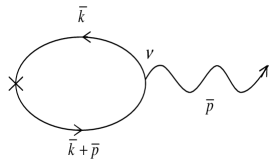
Figure 1: One-loop graph contributing to the anomaly in the chiral current. The solid lines represent fermions, the wavy line a photon and the cross denotes the divergence of the chiral current.

The calculation of the anomaly is best carried out in the real time formalism. First, we note that, in the case of the Schwinger model, we cannot simply take over the form of the fermion propagator from (44). This is because, for a massless fermion in $1+1$ dimensions, the non-dynamical component of the fermion is, in fact, decoupled from the dynamical one as is obvious from (46). As a result, even at zero temperature, the form of the propagator has the form (with the Feynman prescription understood, see also (30))

$$iS(\bar{p}) = \frac{i}{-(2\bar{p}_{0}+\bar{p}_{1})\bar{p}_{1}}\left(\begin{array}[]{cc}-\bar{p}_{1}&0\\ 0&2\bar{p}_{0}+\bar{p}_{1}\end{array}\right)=\left(\begin{array}[]{cc}\frac{i}{2\bar{p}_{0}+\bar{p}_{1}}&0\\ 0&-\frac{i}{\bar{p}_{1}}\end{array}\right)$$ (55)

$$= \frac{i}{2\bar{p}_{0}+\bar{p}_{1}}P^{+}-\frac{i}{\bar{p}_{1}}P^{-}.$$ (56)

As in (31), we note here that this propagator can also be written as

$$iS(\bar{p})=\frac{i\bar{\gamma}^{\mu}\bar{p}_{\mu}(\bar{\gamma}^{0}-\bar{\gamma}^{1})}{-(2\bar{p}_{0}+\bar{p}_{1})\bar{p}_{1}},$$ (57)

which reflects the propagator relations between the conventional quantization and the light-front quantization from the point of view of a coordinate transformation.

The zero temperature anomaly can be calculated using the component fields (which is what is conventionally done in the light-front studies). However, we wish to point out that it is equally convenient to carry out the light-front calculations using the full propagator and the complete vertex of the theory. Both lead to the same result, however, using the full fermion propagator and the complete vertex, one can avoid subtleties arising from regularization. To demonstrate this, let us calculate the zero temperature anomaly in the Schwinger model using the full propagator in (57) and the complete vertex in (46). We note from Fig. 1 that the zero temperature amplitude has the form

$$= -e^{2}\int\frac{d^{2}\bar{k}}{(2\pi)^{2}}\,{\rm Tr}\,(\bar{\gamma}^{0}-\bar{\gamma}^{1})\bar{\gamma}_{5}\bar{p}\!\!\!/S(\bar{k})(\bar{\gamma}^{0}-\bar{\gamma}^{1})\bar{\gamma}^{\nu}S(\bar{k}+\bar{p})$$ (58)

$$= -e^{2}\int\frac{d^{2}\bar{k}}{(2\pi)^{2}}\,{\rm Tr}\,\bar{\gamma}_{5}\bar{p}\!\!\!/\bar{k}\!\!\!/\bar{\gamma}^{\nu}(\bar{k}\!\!\!/+\bar{p}\!\!\!/)\,\frac{1}{\bar{k}^{2}(\bar{k}+\bar{p})^{2}}.$$

Here, we have used the form of the full propagator in (57), the notation

$$\bar{k}^{2}=-(2\bar{k}_{0}+\bar{k}_{1})\bar{k}_{1},$$ (59)

as well as the identity

$$(\bar{\gamma}^{0}-\bar{\gamma}^{1})^{2}=1.$$ (60)

There are several things to note from Eq. (58). First, the form of the integrand is the same as would be obtained in the conventional quantization except for barred quantities. However, since scalar quantities are unchanged under the coordinate transformation (2) and vectors transform in a simple manner, we expect the results to be quite similar to the standard result. In fact, the fermion trace leads to the same result in the barred variables. Normally, the light-front integrals have to be treated with care, but with the full propagator, we note that we can make a change of variables of integration (basically, the inverse redefinition of (2))

$$\bar{k}_{0}=k_{0},\quad\bar{k}_{3}=-k_{0}+k_{3},$$ (61)

which allows us to use standard dimensional regularization (in this case, of course, the result turns out to be finite because of gauge invariance) leading to the value of the amplitude

$$-\frac{e^{2}}{\pi}\bar{\epsilon}^{\mu\nu}\bar{p}_{\mu},$$ (62)

which determines that the anomaly in the chiral current, at zero temperature, is given by

$$\bar{\partial}_{\mu}\bar{\jmath}_{5}^{\mu}=-\frac{e^{2}}{2\pi}\bar{\epsilon}^{\mu\nu}\bar{F}_{\mu\nu}.$$ (63)

To calculate the thermal correction to the anomaly, we note that in the imaginary time formalism, the fermion propagator has the form (see Eq. (56))

$$S^{(\beta)}(\bar{p})=-\frac{1}{2\bar{p}_{0}+\bar{p}_{1}}P^{+}+\frac{1}{\bar{p}_{1}}P^{-},$$ (64)

with $\bar{p}_{0}=\frac{(2n+1)i\pi}{\beta}$. For the calculation of the anomaly, however, the real time formalism is more suitable and the propagator, in this case, is given by (we give only the $++$ component which is relevant)

$$iS_{++}^{(\beta)}(\bar{p})=\bar{\gamma}^{\mu}\bar{p}_{\mu}(\bar{\gamma}^{0}-\bar{\gamma}^{1})\left(\frac{i}{-(2\bar{p}_{0}+\bar{p}_{1})\bar{p}_{1}+i\epsilon}-P^{+}2\pi n_{F}(|\bar{p}_{0}|)\delta((2\bar{p}_{0}+\bar{p}_{1})\bar{p}_{1})\right),$$ (65)

where $n_{F}$ represents the fermion distribution function defined in (45). The interesting thing to note from (65) is the presence of the projection operator $P^{+}$ in the thermal term. This simply reflects the fact that the fermion component $\psi_{-}$ is nondynamical and, as a consequence, does not thermalize. This is also reflected in the form of the propagator (64) in the imaginary time formalism where the component involving $P^{-}$ has no $\bar{p}_{0}$ dependence and, consequently, does not have any temperature dependence. We would like to emphasize that the propagator in (65) also results if we start with a massive fermion propagator as in (44) (for $1+1$ dimensions) and take the limit $m\rightarrow 0$.

With the form of the propagator in (65), we can now calculate the temperature dependence of the amplitude in Fig. 1. Once again, the calculations can be done in components or with the full propagator and both yield the same result. If we take the full propagator and the vertex, the temperature dependent part of the amplitude can be calculated very easily. The terms linear in the fermion distribution function (with a little algebra) take the form

$$\sim\int\frac{d^{2}\bar{k}}{(2\pi)^{2}}\,\bar{\epsilon}^{\mu\nu}\bar{k}_{\mu}\,n_{F}(|\bar{k}_{0}|)\delta(\bar{k}^{2})=0.$$ (66)

Similarly, the terms in the amplitude quadratic in the fermion distribution function give (even before doing the Dirac trace)

$$\sim\int\frac{d^{2}\bar{k}}{(2\pi)^{2}}\,{\rm Tr}\,(1+\bar{\gamma}_{5})\bar{k}\!\!\!/\bar{\gamma}^{\nu}(\bar{p}^{2}+2\bar{p}\cdot\bar{k})n_{F}(|\bar{k}_{0}|)n_{F}(|\bar{k}_{0}+\bar{p}_{0}|)\delta(\bar{k}^{2})\delta((\bar{k}+\bar{p})^{2})=0.$$ (67)

This shows that the anomaly is unchanged by temperature corrections which is, of course, well known in the conventional quantization das ; karev ; itoyama , but holds true also in the light-front quantization. Since the chiral anomaly is directly related to the mass of the photon in the Schwinger model, this also implies that the photon mass is unchanged by the temperature corrections.

Let us next calculate the temperature dependent correction to the self-energy of the photon. The photon self-energy is a second rank symmetric tensor and it is easy to see from the form of the amplitude that

$$\bar{\Pi}^{00(\beta)}(\bar{p})=2\bar{\Pi}^{01(\beta)}(\bar{p})=2\bar{\Pi}^{10(\beta)}(\bar{p})=4\bar{\Pi}^{11(\beta)}(\bar{p}),$$ (68)

so that only one independent component needs to be calculated. The calculation is straightforward and leads to

$$\bar{\Pi}^{01(\beta)}(\bar{p})=-e^{2}\delta(2\bar{p}_{0}+\bar{p}_{1})\int d\bar{k}_{1}\,{\rm sgn}(\bar{k}_{1}){\rm sgn}(\bar{k}_{1}+\bar{p}_{1})\left(n_{F}(\frac{|\bar{k}_{1}|}{2})+n_{F}(\frac{|\bar{k}_{1}+\bar{p}_{1}|}{2})-2n_{F}(\frac{|\bar{k}_{1}|}{2})n_{F}(\frac{|\bar{k}_{1}+\bar{p}_{1}|}{2})\right).$$ (69)

There are several things to note from Eqs. (68)-(69). First of all, it is clear that the self-energy is gauge invariant (transverse). Second taking the dual (in one of the indices) and contracting with the external momentum gives zero, which shows again that the anomaly has no temperature dependent contribution. The presence of the delta function structure in the amplitude is a reflection of the non-analyticity in amplitudes at finite temperature and the amplitude in (69) reflects the structure found in the conventionally quantized theory adilson . However, there is a difference in the sense that the amplitude in Eq. (69) shows only one delta function structure whereas in the conventionally quantized theory, there are two independent delta function structures present. This difference can be traced back to the fact that in the light-front quantization of the Schwinger model, only one of the fermion components thermalizes (which is how one delta function structure arises and which also reflects the fact that light-front quantization inherently breaks parity invariance dharam ). Thus, it would seem that there is finally a difference between the light-front and conventionally quantized theories. Let us recall, however, that the photon is massive in the Schwinger model whereas the thermal self-energies in (68), (69) as well as those in adilson contribute nontrivially only when $2\bar{p}_{0}+\bar{p}_{1}=0$ (or $p_{0}\pm p_{1}=0$ in adilson ). Consequently, for a massive photon on-shell, the thermal self-energies vanish in both conventional as well as light-front quantizations. On the other hand, they are non-vanishing and distinct in the two quantizations away from the physical mass-shell. This calculation can be easily generalized to the thermal $n$-point amplitudes for the photon completely along the lines discussed in adilson . Without going into technical details, we simply summarize our result here. The non-vanishing components of the thermal $n$-point amplitude have an identical structure to that in adilson except that we find only a single product of delta functions of the kind in (69) (which again reflects that only one fermion component thermalizes). Once again, this shows that these thermal amplitudes vanish on-shell for a massive photon as is the case in adilson , but off-shell, the two results are quite distinct.

An important aspect of the light-front quantization is that it allows for a simpler description of questions involving bound states. From our discussion above, since the on-shell thermal self-energy for the photon vanishes, the equation for the bound state of fermions (and, therefore, the solution) should not change at finite temperature. This can also be seen quantitatively as follows. In the axial gauge (which is conventionally used in the study of bound states in this problem), $\bar{A}_{1}=0$, the photon equation becomes a constraint. In fact, the Lagrangian density for a massive fermion (the mass parameter can be taken to zero) interacting with an electromagnetic potential in the axial gauge takes the form

$${\cal L}=\frac{1}{2}(\bar{\partial}_{1}\bar{A}_{0})^{2}+i\psi_{+}^{\dagger}(2\bar{\partial}_{0}+\bar{\partial}_{1})\psi_{+}-i\psi_{-}^{\dagger}\bar{\partial}_{1}\psi_{-}+m\psi_{+}^{\dagger}\bar{\gamma}^{1}\psi_{-}-m\psi_{-}^{\dagger}\bar{\gamma}^{1}\psi_{+}+2e\psi_{+}^{\dagger}\psi_{+}\bar{A}_{0},$$ (70)

leading to the equation for the photon of the form

$$\bar{A}_{0}=\frac{2e}{(\bar{\partial}_{1})^{2}}\,\psi_{+}^{\dagger}\psi_{+}.$$ (71)

Eliminating this constraint, the Hamiltonian takes the form

$$H=\int d\bar{x}^{1}\left[-i\psi_{+}^{\dagger}\bar{\partial}_{1}\psi_{+}+im^{2}\psi_{+}^{\dagger}\frac{1}{\bar{\partial}_{1}}\psi_{+}-2e^{2}\psi_{+}^{\dagger}\psi_{+}\frac{1}{(\bar{\partial}_{1})^{2}}\psi_{+}^{\dagger}\psi_{+}\right].$$ (72)

The self-energy term depends on $\frac{1}{(\bar{\partial}_{1})^{2}}$, which does not change at finite temperature. As a result, the bound state equation as well as the solution remains unchanged at finite temperature.

Another interesting quantity that can be calculated in this model is the fermion condensate. There are various ways of calculating this at finite temperaturejayawardene ; smilga . However, we follow, for simplicity, the method in smilga which uses bosonization and is relatively straightforward. The bosonized version of the Schwinger model describes a free, massive scalar field

$${\cal L}=\frac{1}{2}\bar{\partial}_{\mu}\phi\bar{\partial}^{\mu}\phi-\frac{m_{\rm ph}^{2}}{2}\phi^{2},$$ (73)

where

$$m_{\rm ph}=\frac{e}{\sqrt{\pi}}.$$ (74)

The correspondence between the bosonic and the fermionic degrees of freedom, among other things, leads to the identification

$$\bar{\psi}\psi=-\frac{m_{\rm ph}e^{\gamma}}{2\pi}:\cos\sqrt{4\pi}\phi:\,.$$ (75)

Here $\gamma$ represents Euler’s constant and the “colons” stand for normal ordering with respect to the scalar annihilation and creation operators. It is straightforward to calculate from this the value of the fermion condensate at zero temperature,

$$\langle\bar{\psi}\psi\rangle_{T=0}=-\frac{m_{\rm ph}e^{\gamma}}{2\pi},$$ (76)

since the normal ordered fields lead to trivial vacuum expectation values at zero temperature. At finite temperature, on the other hand, the condensate has the form

$$\langle\bar{\psi}\psi\rangle_{T}=\langle\bar{\psi}\psi\rangle_{T=0}\,e^{-2i\pi(G^{(\beta)}(0)-G(0))}.$$ (77)

Using the representation for the scalar propagator in (10) (in $1+1$ dimensions and using only the $++$ component), it is easy to see that

$$iG^{(\beta)}(0)-iG(0)=\frac{1}{2\pi}\int_{0}^{\infty}\frac{d\bar{k}_{1}}{\bar{k}_{1}}\,\frac{1}{e^{\beta(\bar{k}_{1}+\frac{m_{\rm ph}^{2}}{\bar{k}_{1}})}-1}.$$ (78)

The integral in (78) cannot be evaluated in closed form in general. However, for low temperatures (large $\beta$), it has the form gradshteyn

$$iG^{(\beta)}(0)-iG(0) \approx \frac{1}{2\pi}\int_{0}^{\infty}\frac{d\bar{k}_{1}}{\bar{k}_{1}}\,e^{-\beta(\bar{k}_{1}+\frac{m_{\rm ph}^{2}}{\bar{k}_{1}})}=\frac{1}{\pi}K_{0}(\beta m_{\rm ph})$$ (79)

$$\rightarrow \sqrt{\frac{T}{2\pi m_{\rm ph}}}\,e^{-\frac{m_{\rm ph}}{T}}.$$

On the other hand, at high temperatures (small $\beta$), we have gradshteyn

$$iG^{(\beta)}(0)-iG(0) = \frac{1}{2\pi}\sum_{n=1}^{\infty}\int_{0}^{\infty}\frac{d\bar{k}_{1}}{\bar{k}_{1}}\,e^{-n\beta(\bar{k}_{1}+\frac{m_{\rm ph}^{2}}{\bar{k}_{1}})}=\frac{1}{\pi}\sum_{n=1}^{\infty}K_{0}(n\beta m_{\rm ph})$$ (80)

$$\rightarrow \frac{T}{2m_{\rm ph}}+\frac{1}{2\pi}\ln\frac{m_{\rm ph}}{4\pi T}+\frac{\gamma}{2\pi}.$$

Using Eq. (79) in (77), we obtain the value of the condensate at low temperatures to be

$$\langle\bar{\psi}\psi\rangle_{T}\approx\langle\bar{\psi}\psi\rangle_{T=0}\left(1-\sqrt{\frac{2\pi T}{m_{\rm ph}}}e^{-\frac{m_{\rm ph}}{T}}\right),$$ (81)

whereas Eq. (80) leads to the high temperature value of the condensate as

$$\langle\bar{\psi}\psi\rangle_{T}\approx-2Te^{-\frac{\pi T}{m_{\rm ph}}}.$$ (82)

These are precisely the values of the condensates obtained earlier using the conventional quantization jayawardene ; smilga and we see once again that the results in the two quantizations coincide even at finite temperature.

V Conclusion

In this paper, we have studied the light-front Schwinger model in detail following the recent proposal alves . We have shown, with the calculation of the anomaly at zero temperature, that it may be more efficient to calculate with the full theory when fermions are involved. We have shown that the thermal corrections to the anomaly vanish, consistent with the expectation from the calculations with the conventional quantization. The thermal photon self-energy is shown to have the expected non-analytic behavior, but coincides with the result from the conventional quantization only on-shell. We have shown that the bound state equations are unchanged at non zero temperature and that the fermion condensate has the same value at finite temperature as in conventional quantization. In fact, if light-front quantization is viewed as quantization in a general coordinate system weldon , the physical S-matrix elements will be naively expected to be the same in both light-front as well as conventional quantizations. At zero temperature, particularly, such an equivalence in the physical sector, even though expected chang , is hard to prove rigorously owing to subtleties involving regularization of ultraviolet divergences brodsky2 . However, the thermal contributions are free from ultraviolet divergences and, consequently, one may expect equivalence of physical thermal amplitudes in the two quantizations. Our calculations, in the Schwinger model, explicitly exhibit this feature in this model and furthermore show that off-shell Greens functions in the two quantizations need not be the same.

Acknowledgment:

One of us (AD) would like to thank Prof. J. Frenkel for helpful discussions. This work was supported in part by US DOE Grant number DE-FG 02-91ER40685.

Note added: In a later paper new , complete thermal equivalence between conventional quantization and light-front quantization is claimed where the general proof is based on formal arguments. In this paper, on the other hand, we have explicitly evaluated the thermal amplitudes in a given theory, namely, the Schwinger model and our calculation shows that the off-shell thermal Green’s functions, in this theory, are different in the two quantizations. It is quite likely, therefore, that some of the assumptions that go into the general proof are violated in this model, as our calculation seems to suggest.

References

- (1) V. S. Alves, A. Das and S. Perez, Phys. Rev. D66, 125008 (2002).
- (2) There are numerous papers on the subject to list individually. Therefore, we list only the following review papers which contain an exhaustive list of references to the subject. M. Burkhadt, Adv. Nucl. Phys. 23, 1 (1996); S. J. Brodsky, H. C. Pauli and S. S. Pinsky, Phys. Rep. 301, 299 (1998); K. Yamawaki, “Zero mode problem on the light-front”, hep-th/9802037; T. Heinzl, “Light-cone quantization: Foundations and applications”, hep-th/0008096.
- (3) H. A. Weldon, “Thermal field theory and generalized light front quantization”, hep-ph/0302147, to be published in Phys. Rev. D.
- (4) H. A. Weldon, “Thermal self-energies using light-front quantization”, hep-ph/0304096, to be published in Phys. Rev. D.
- (5) J. Schwinger, Phys. Rev. 128, 2425 (1962).
- (6) B. Klaiber, in Lectures in Theoretical Physics, Boulder 1967 (Gordon and Breach, New York, 1968).
- (7) E. Abdalla, M. C. B. Abdalla and K. D. Rothe, Non-perturbative Methods in Two Dimensional Quantum Field Theories (World Scientific, Singapore, 2001).
- (8) See, for example, H. Bergknoff, Nucl. Phys. B122, 215 (1977); T. Eller, H. C. Pauli and S. Brodsky, Phys. Rev. D35, 1493 (1987) as well as the review article by A. Harindranath, An Introduction to Light-front Dynamics for Pedestrians, hep-ph/9612244.
- (9) J. Kapusta, Finite Temperature Field Theory (Cambridge University Press, Cambridge, England, 1989).
- (10) M. Le Bellac, Thermal Field Theory (Cambridge University Press, Cambridge, England, 1996).
- (11) A. Das, Finite Temperature Field Theory (World Scientific, Singapore, 1997).
- (12) A. Das and A. Karev, Phys. Rev. D36, 623 (1987).
- (13) The temperature independence of the anomaly in dimensions was first shown in H. Itoyama and A. H. Muller, Nuc. Phys. B218, 349 (1983).
- (14) H. A. Weldon, Phys. Rev. D28, 2007 (1983); Phys. Rev. D47, 594 (1993).
- (15) P. F. Bedaque and A. Das, Phys. Rev. D47, 601 (1993).
- (16) A. Das and M. Hott, Phys. Rev. D50, 6655 (1994).
- (17) A. Das and A. J. da Silva, Phys. Rev. D59, 105011 (1999).
- (18) D. V. Ahluwalia and M. Sawicki, Phys. Rev. D47, 5161 (1993) and references therein.
- (19) Y-C. Kao, UCB-PTH 83/14 (unpublished); C. Jayewardena, Helv. Phys. Acta 61, 636 (1988); I. Sachs and A. Wipf, Helv. Phys. Acta 65, 652 (1992); Y-C. Kao, Mod. Phys. Lett. A7, 1411 (1992).
- (20) A. V. Smilga, Phys. Lett. B278, 371 (1992).
- (21) A. Liguori, M. Mintchev and L. Pilo, Nucl. Phys. B569, 577 (2000).
- (22) P. P. Srivastava and S. J. Brodsky, Phys. Rev. D64, 045006 (2001).
- (23) I. S. Gradshteyn and I. M. Ryzhik, Table of Integrals, Series and Products (Academic Press, New York, 1980).
- (24) S. J. Chang, R. G. Root, T-M. Yan, Phys. Rev. D7, 1133 (1973); S. J. Chang, T-M. Yan, Phys. Rev. D7, 1147 (1973).
- (25) The equivalence is established only case by case and there is no known counter example (S. Brodsky, private communication).
- (26) A. N. Kvinikhidze and B. Blakleider, “Equivalence of light-front and conventional thermal field theory”, hep-th/0305115.