In this paper we study general properties of noncommutative field theories obtained from the Seiberg-Witten limit of string theories in the presence of an external $B$-field. We analyze the extension of the Wightman axioms to this context and explore their consequences, in particular we present a proof of the CPT theorem for theories with space-space noncommutativity. We analyze as well questions associated to the spin-statistics connections, and show that noncommutative $\mathcal{N}=4$, U(1) gauge theory can be softly broken to $\mathcal{N}=0$ satisfying the axioms and providing an example where the Wilsonian low energy effective action can be constructed without UV/IR problems, after a judicious choice of soft breaking parameters is made. We also assess the phenomenological prospects of such a theory, which are in fact rather negative.

1 Introduction and motivation

Noncommutative geometry has had a profound influence in Mathematics (cf. [1]). Also in Physics it has had an effect in a number of subjects ranging from applications to the integer and fractional quantum Hall effects [2, 3] in condensed matter physics [4], to the noncommutative formulation of the standard model by Connes and Lott [5] (see also [6] for a review).

In string theory the use of noncommutative geometry was pioneered by Witten [7] in his formulation of open string field theory. Compactifications of string and M-theory on noncommutative tori were studied in [8]. Shortly after this, Seiberg and Witten [9] realized that a certain class of quantum field theories on noncommutative Minkowski space-times can be obtained as a particular low energy limit of open strings in the presence of a constant NS-NS $B_{\mu\nu}$ field (see also [10]). This result generated a flurry of activity in the study of quantum field theories in noncommutative spaces (see [11] for reviews). Part of the interest has been aimed at getting new insights into the regularization and renormalization of quantum field theories in this novel framework. In fact, many features of ordinary (commutative) field theories have found rich analogues in the noncommutative context [12].

The noncommutative field theories obtained from string theory via the Seiberg-Witten limit are neither local nor Lorentz invariant, since the fields in the action appear multiplied with Moyal products. Locality, together with Lorentz invariance, have been traditionally considered to be two of the holy principles in a quantum field theory. With few exceptions, there has been little motivation to try to extend the principles of quantum field theory to non-local (or non-Lorentz invariant) theories. Although in general allowing for non-locality in quantum field theory creates havoc, the Seiberg-Witten limit yields a very specific class of non-local theories where, together with some unusual features, some of the desirable properties of local theories are preserved. Therefore it has been a challenge to understand the consequences, both theoretical and phenomenological, of these theories [13].

The first unexpected property of noncommutative field theories was pointed out by Minwalla, van Raamsdonk and Seiberg [14]. These authors realized that quantum theories on noncommutative spaces are afflicted from an endemic mixing of ultraviolet and infrared divergences. Even in massive theories the existence of ultraviolet divergences induce infrared problems [15]. As a consequence the Wilsonian approach to field theory seems to break down: integrating out high-energy degrees of freedom produces unexpected low-energy divergences, inducing in the infrared operators of negative dimension. This lack of decoupling of high energy modes seem to doom these theories from any phenomenological perspective (see Section 5).

In ordinary Quantum Field Theory there are important consequences that follow from the general principles of relativistic invariance and locality, which do not necessarily extend to the noncommutative case. Results like the CPT theorem [16, 17, 18] and the spin-statistic connection [19] will not necessarily hold. Similarly, questions concerning the existence of an $S$-matrix, its unitarity and the notion of asymptotic completeness are in need of drastic revisions. In Refs. [20, 21, 22, 23] the CPT invariance of noncommutative field theories was studied, and it was concluded that the CPT theorem holds, both in the case of space-space and time-space noncommutativity. However, this analysis deals with the tree-level action and it is not sensitive to possible problems arising from quantum corrections. In the case of noncommutative field theories problems might appear in the form of unitarity violations or UV/IR mixing. In particular, the mixing of scales may jeopardize the tempered nature of the Wightman functions as distributions. These issues might demand a revision of the proof of the CPT theorem presented in [23].

In the present paper we will study in detail some general properties of noncommutative quantum field theories, such as the CPT theorem and the spin-statistics connection, as well as the possibility of constructing theories that are well-defined in the infrared. We will propose an axiomatic formulation leading to a proof of the CPT theorem along the lines of the one given by Jost for ordinary theories [17, 18]. In this axiomatic formulation the vacuum expectation value of the Heisenberg fields should define tempered distributions. This mathematical condition imposes non-trivial restrictions on the correlation functions both in the ultraviolet and the infrared. In order to give meaning to noncommutative gauge theories in the infrared we present a detailed analysis of noncommutative U(1)_⋆ gauge theory with $\mathcal{N}=4$ supersymmetry softly broken to $\mathcal{N}=0$ in a way that preserves finiteness in the ultraviolet and that leads to a well-defined theory at low energies. The resulting theory provides correlation functions that behave like tempered distributions, while in the infrared we recover the free Maxwell theory. We show that the theory defined in this way satisfies the proposed axioms and assess its phenomenological viability.

This paper is organized as follows: in Section 2 we briefly review the Seiberg-Witten limit, and analyze heuristically when CPT-invariance and unitarity of the $S$-matrix are expected to hold. In Section 3 we adapt the Wightman axioms to the noncommutative context. In particular we analyze the issue of microscopic causality [17]. In Section 4 we show that with the modified axioms it is still possible to prove the CPT theorem but, in the general case, the connection between spin and statistics is not guaranteed. In Section 5 we analyze the softly broken $\mathcal{N}=4$ noncommutative U(1)_⋆ gauge theory and show that it is possible to formulate it in such a way that the adapted axioms are satisfied at least in perturbation theory. We also make some general remarks on the possible phenomenological perspectives of noncommutative field theories. Finally, our conclusions are presented in Section 6.

A final remark is in order before closing this introduction. We are going to study the class of noncommutative field theories obtained from the Seiberg-Witten limit of string theories in the presence of a constant $B$-field. These theories are defined quantum-mechanically in perturbation theory in terms of their Feynman rules which follow from the parent string theory. For reasons to be explained in the next section, we consider here only the case of space-space noncommutativity. However, from a purely field-theoretical point of view, other procedures can be envisaged to quantize them. In particular, the authors of Ref. [25], motivated by the work of [26], proposed a different way to look at noncommutative theories that leads to a unitary $S$-matrix and, if uncertainty relations for the space-time coordinates are implemented, they claim to obtain not only a unitary theory but also one that is ultraviolet-finite. In [27] the authors start with Dyson’s formula to define the Green functions, and by a careful analysis of the passage from time-ordered products to Wick products, they conclude that the Feynman rules change when there is time-space noncommutativity in a way that preserves perturbative unitarity. For space-space noncommutativity the Feynman rules are the same as those obtained from string theory via the Seiberg-Witten limit.

2 Heuristic considerations

Noncommutative field theories, i.e. theories with ordinary products replaced by Moyal products, are from a quantum point of view theories of dipoles [28]. Since the elementary excitations are extended objects, the resulting theory is nonlocal and the scale of non-locality is set by the length of these dipoles.

This fact is easy to visualize in the cases where noncommutative theories arise as effective description of the dynamics in a certain limit. In Ref. [9] it was shown how noncommutative field theories are obtained as a particular low-energy limit of open string theory on D-brane backgrounds in the presence of constant NS-NS $B$-field. In this case, the endpoints of the open strings behave as electric charges in the presence of an external magnetic field $B_{\mu\nu}$ resulting in a polarization of the open strings. Labelling by $i=1,\ldots,p$ the D-brane directions, the difference between the zero modes of the string endpoints is given by ($B_{0i}=0$) [10]

$$\Delta X^{i}=X^{i}(\tau,0)-X^{i}(\tau,\pi)=(2\pi\alpha^{\prime})^{2}g^{ij}B_{jk}p^{k},$$ (2.1)

where $g_{\mu\nu}$ is the closed string ($\sigma$-model) metric and $p^{\mu}$ is the momentum of the string. In the ordinary low-energy limit ($\alpha^{\prime}\rightarrow 0$, $g_{\mu\nu}$, $B_{\mu\nu}$ fixed) the distance $|\Delta X|$ goes to zero and the effective dynamics is described by a theory of particles, i.e. by a commutative quantum field theory.

There are, however, other possibilities of decoupling the massive modes without collapsing at the same time the length of the open strings. Seiberg and Witten proposed to consider a low energy limit $\alpha^{\prime}\rightarrow 0$ where both $B_{ij}$ and the open string metric

$$G_{ij}=-(2\pi\alpha^{\prime})^{2}(Bg^{-1}B)_{ij}$$ (2.2)

are kept fixed. Introducing the notation $\theta^{ij}=(B^{-1})^{ij}$, the separation between the string endpoints can be expressed as

$$\Delta X^{i}=\theta^{ij}G_{jk}p^{k},$$ (2.3)

fixed in the low energy limit. The resulting low-energy effective theory is a noncommutative field theory with noncommutative parameter $\theta^{ij}$.

The Seiberg-Witten limit can be viewed as a stringy analog of the projection onto the lowest Landau level in a system of electrons in a magnetic field. Indeed, the condition fixing the open string metric $G_{\mu\nu}$ in the low-energy limit is equivalent to considering a large $B$-field limit in which the interaction of the external field with the end-points of the string dominates the worldsheet dynamics. In more physical term, Eq. (2.1) can be interpreted as a competition between the Lorentz force exerted on the endpoints of the string and the tension that tends to collapse the string to zero size. The Seiberg-Witten limit corresponds to making the string rigid by taking the tension to infinity (thus decoupling the excited states) while at the same time keeping the $B$-field large in string units, in such a way that the length of the string is kept constant.

The previous analysis was confined to situations in which the $B_{0i}$ components are set to zero. This results in a noncommutative field theory with only space-space noncommutativity. From a purely field-theoretical point of view it is possible to consider also noncommutative theories where the time coordinate does not commute with the spatial ones, i.e. $\theta^{i0}\neq 0$. In this case, however, non-locality is accompanied by a breakdown of unitarity reflected in the fact that the optical theorem is not satisfied [29, 30]. In addition there is no well-defined Hamiltonian formalism (see, however, [25]).

Noncommutative field theories with time-space noncommutativity cannot be obtained from string theory in a limit in which strings are completely decoupled. One can try to obtain these kind of theories by looking for a decoupling limit of string theory in D-brane backgrounds in the presence of $B$-fields with $B_{0i}\neq 0$. That the existence of such a decoupling limit is not inmediate can be envisaged by noticing that having $B_{0i}\neq 0$ is equivalent to a nonvanishing electric field on the brane, and that in this case the electric field has to be smaller that the critical value [31]

$$E<E_{\rm crit}={1\over 2\pi\alpha^{\prime}}.$$ (2.4)

For fields larger than $E_{\rm crit}$ the background decays via the formation of pairs of open strings in a stringy version of the Schwinger mechanism. A partial decoupling limit can be achieved in the limit $E\rightarrow E_{\rm crit}$ while keeping $\theta^{\mu\nu}$ and the string tension fixed. In this limit closed strings decople from open strings while the latter ones remain in the spectrum [32]. Actually, the optical theorem can be formally restored by taking into account the interchange of undecoupled string states in intermediate channels, although they are both tachyonic and have negative norm [30].

In order to avoid these problems, in the following we restrict ourselves to theories with space-space noncommutativity. Then the existence of a parent string theory provides a good guiding principle to study their properties. The parent string theory also provides a ultraviolet completion where non-locality is realized by string fuzziness.

The CPT theorem in string theory has been investigated by several groups [33]. If the parent string theory satisfies the CPT theorem in perturbation theory, since the constant background $B$-field is CPT-even, it is reasonable to expect that the noncommutative quantum field theory obtained in the Seiberg-Witten limit should also preserve CPT. At the level of the noncommutative field theory it is also expected to have CPT-invariance for theories with $\theta^{0i}=0$. As discussed above, these kind of noncommutative theories preserve perturbative unitarity. In ordinary quantum field theory there is an intimate connection between unitarity and CPT-invariance. Indeed, if the condition of asymptotic completeness holds, it can be seen using either the Yang-Feldman relation [34] or the Haag-Ruelle scattering theory [35] that the $S$-matrix can be written in terms of the CPT operator of the complete theory $\Theta$ and the corresponding one for the asymptotic theory $\Theta_{0}$ (see also [36])

$$S=\Theta^{-1}\Theta_{0}.$$ (2.5)

The unitarity of the $S$-matrix follows then from the antiunitarity of $\Theta$ and $\Theta_{0}$. Therefore a theory with CPT invariance is likely to be unitary.

Motivated by these heuristic arguments we proceed to construct the CPT theorem along the lines of the proof given in [18]. As a first step we attempt an axiomatic formulation of noncommutative field theories as a modification of the Wightman axioms [37, 38, 39].

3 Modified constructions

Compared to ordinary theories, two basic features of noncommutative theories are their non-locality and the breaking of Lorentz invariance due to the presence of the antisymmetric tensor $\theta^{\mu\nu}$. In the following we will take it of the form

$$\theta^{\mu\nu}=\left(\begin{array}[]{cccc}0&\theta_{e}&0&0\\ -\theta_{e}&0&0&0\\ 0&0&0&\theta_{m}\\ 0&0&-\theta_{m}&0\end{array}\right),$$ (3.5)

with $\theta_{e},\theta_{m}\in\mathbb{R}$. The Wightman axioms have to be modified in order to accommodate noncommutativity and reduced Poincaré invariance. Eventually we will be interested in theories with space-space noncommutativity $\theta_{e}=0$. Nevertheless, for most of this section we will keep $\theta_{e}$ explicitly.

3.1 Symmetries of noncommutative field theories

The commutation relations for the coordinates $[x^{\mu},x^{\nu}]=i\theta^{\mu\nu}$ are not preserved by the Lorentz group O(1,3) although they are indeed left invariant by the group of rigid translations $x^{\mu}\rightarrow x^{\mu}+a^{\mu}$ with $a^{\mu}\in\mathbb{R}$. Using (3.5) it is straightforward to find that the largest subgroup of O(1,3) leaving invariant the commutation relations is SO(1,1)$\times$SO(2), where the SO(1,1) factor acts on the “electrical” coordinates $x_{e}=(x^{0},x^{1})$ whereas SO(2) rotates the “magnetic” ones $\vec{x}_{m}=(x^{2},x^{3})$. In the case of space-space noncommutativity ($\theta_{e}=0$) this group is enhanced to O(1,1)$\times$ SO(2). Since we will be mostly concerned about this latter case, we will take the symmetry group of the noncommutative theory to be $\mathfrak{P}=[\mbox{O(1,1)}\times\mbox{SO(2)}]\rtimes\mathcal{T}_{4}$,where $\mathcal{T}_{4}$ is the group of translations.

The representation theory of O(1,1)$\times$SO(2) shares many common features with that of the Lorentz group O(1,3). Representations of SO(2) are parametrized by the angle $\varphi\in[0,2\pi]$. The O(1,1) factor has a richer structure. As in the standard case, it has four sheets

$$\mathfrak{L}_{\pm}^{\uparrow}: \hskip 14.22636pt\det{\Lambda}=\pm 1;\hskip 7.11317pt\Lambda^{0}_{\,\,0}\geq 1,$$ (3.6)

$$\mathfrak{L}_{\pm}^{\downarrow}: \hskip 14.22636pt\det{\Lambda}=\pm 1;\hskip 7.11317pt\Lambda^{0}_{\,\,0}\leq-1.$$ (3.7)

The elements of the four sheets can be expressed as a product of an element of $\mathfrak{L}_{+}^{\uparrow}$ and one of the three discrete transformations inverting one or the two electric coordinates

$$\mathfrak{L}_{+}^{\downarrow}=\mathfrak{L}_{+}^{\uparrow}I_{\rm st},\hskip 28.45274pt\mathfrak{L}_{-}^{\uparrow}=\mathfrak{L}_{+}^{\uparrow}I_{\rm s},\hskip 28.45274pt\mathfrak{L}_{-}^{\downarrow}=\mathfrak{L}_{+}^{\uparrow}I_{\rm t}$$ (3.8)

where

$$I_{\rm st}=\left(\begin{array}[]{cc}-1&0\\ 0&-1\end{array}\right),\hskip 28.45274ptI_{\rm s}=\left(\begin{array}[]{cc}1&0\\ 0&-1\end{array}\right),\hskip 28.45274ptI_{\rm t}=\left(\begin{array}[]{cc}-1&0\\ 0&1\end{array}\right).$$ (3.15)

Each element of $\mathfrak{L}_{+}^{\uparrow}$ is parametrized by a single number $\gamma\in\mathbb{R}$, the rapidity of the boosts along $x^{1}$

$$\Lambda=\left(\begin{array}[]{cc}\cosh\gamma&\sinh\gamma\\ \sinh\gamma&\cosh\gamma\end{array}\right).$$ (3.18)

The transformations of $x_{e}$ are specially simple introducing null-coordinates $x^{\pm}={1\over\sqrt{2}}(x^{0}\pm x^{1})$. These transform according to

$$\mathfrak{L}_{+}^{\uparrow}:x^{\pm}\longrightarrow e^{\pm\gamma}x^{\pm}$$ (3.19)

together with

$$I_{\rm st}x^{\pm}=-x^{\pm},\hskip 28.45274ptI_{\rm s}x^{\pm}=x^{\mp},\hskip 28.45274ptI_{\rm t}x^{\pm}=-x^{\mp}.$$ (3.20)

Similar to four dimensions, the complexification of O(1,1) connects continuously different sheets. In particular $\mathfrak{L}_{+}^{\uparrow}$ and $\mathfrak{L}_{+}^{\downarrow}$ can be connected by a family of transformations with complex rapidity $\gamma+i\vartheta$ where $0\leq\vartheta\leq\pi$. Denoting $\mathfrak{L}_{+}=\mathfrak{L}_{+}^{\uparrow}\cup\mathfrak{L}_{+}^{\downarrow}\equiv\mbox{SO(1,3)}$ we find

$$\mathfrak{L}_{+}(\mathbb{C})=\mathbb{C}^{*}\equiv\mathbb{C}-\{0\}$$ (3.21)

where the action of $\mathfrak{L}_{+}(\mathbb{C})$ on the coordinates is given by $x^{\pm}\rightarrow zx^{\pm}$, $z\in\mathbb{C}^{*}$. In particular, this result implies that the transformation inverting $x_{e}$ can be continuously connected with the identity using transformations of $\mathfrak{L}_{+}(\mathbb{C})$. At the same time $\vec{x}_{m}$ can also be inverted by a 180 degrees SO(2)-rotation. This result is central in the proof of the CPT theorem (see Section 4).

Representations of SO(1,1) are labelled by a helicity $\lambda\in\mathbb{R}$ and those of SO(2) by the “angular momentum” $j$ ($2j\in\mathbb{Z}$). Any quantity $\Psi^{(j)}_{\lambda}$ in the $(\lambda,j)$ representation of O(1,1)$\times$ SO(2) transforms as

$$\Psi^{(j)}_{\lambda}\longrightarrow e^{\lambda\gamma}\,e^{j\varphi}\,\Psi^{(j)}_{\lambda}.$$ (3.22)

In $\mathfrak{P}$ we can build two Casimir operators with $P_{\mu}$

$$s\equiv(P^{0})^{2}-(P^{1})^{2},\hskip 28.45274ptt\equiv(P^{2})^{2}+(P^{3})^{2},$$ (3.23)

In perturbative calculations in noncommutative field theories these two invariants appear usually in the combinations

$$p^{2}=s-t,\hskip 28.45274ptp\circ p=\theta_{e}^{2}s+\theta_{m}^{2}t.$$ (3.24)

Since by definition $t\geq 0$, the representations of $\mathfrak{P}$ can be classified according to the sign of $s$ into “massless” ($s=0$), “massive” ($s>0$) and “tachyonic” ($s<0$). Since $\mathfrak{P}\subset\mathscr{P}={\rm O}(1,3)\rtimes\mathcal{T}_{4}$, it is important to notice that the type of the representations of $\mathfrak{P}$ do not necessarily coincide with those of $\mathscr{P}$. In particular, from (3.24), we see that “massive” and “massless” representations of $\mathfrak{P}$ can be tachyonic when interpreted as representations of $\mathscr{P}$. On the other hand, any “tachyonic” representation of $\mathfrak{P}$ will be tachyonic with respect to $\mathscr{P}$, but not the other way around.

3.2 Microcausality

The second issue that has to be studied in our attempt to find an axiomatic formulation of noncommutative field theories is the notion of microcausality. In ordinary theories causality is implemented by demanding that fields should commute or anticommute outside their relative light cone. For noncommutative theories there is no structure preserving the four-dimensional Lorentz group O(1,3) and the concept of a light cone is lost.

From our discussion of the symmetries of noncommutative field theories it follows that causality, if preserved at all, must be defined with respect to the O(1,1) factor of the symmetry group. This means that the light cone $x^{2}=0$ is actually replaced by the “light wedge” $V_{+}=\{x\in\mathbb{R}^{1,3}|x_{e}^{2}=0\}$ (see Fig. 1).

Figure 1: The causal wedge $V_{+}$.

This suggests a change in the concept of microcausality by replacing the light cone by the light wedge, so fields will either commute or anticommute whenever their relative coordinate $x-y$ satisfies $(x_{e}-y_{e})^{2}<0$.

In the following, we study a weaker version of this condition, namely under which conditions the vacuum expectation value of the commutator of two noncommutative scalar fields vanishes outside the light wedge. To achieve this we construct a Källén-Lehmann representation for $\langle\Omega|[\phi(x),\phi(y)]|\Omega\rangle$ (with $|\Omega\rangle$ the unique vacuum state of the theory) using invariance under the group $\mathfrak{P}$. Therefore we introduce the [O(1,1)$\times$SO(2)]-invariant measure:

$$d\mu(p)={d^{4}p\over(2\pi)^{4}}\vartheta(p^{0})\,(2\pi)\,\delta(p_{e}^{2}-\alpha^{2})\,(2\pi)\,\delta(\vec{p}_{m}^{\,2}-\beta^{2}).$$ (3.25)

Using a basis of the Hilbert space $\{|j,p_{e},\vec{p}_{m}\rangle\}$, where $j$ is a collective index denoting any other set of quantum numbers needed to specify the state, we write the closure relation

$$1=|\Omega\rangle\langle\Omega|+\sum_{j}\int d\mu(p_{j})|j,p_{e},\vec{p}_{m}\rangle\langle j,p_{e},\vec{p}_{m}|.$$ (3.26)

Starting with $\langle\Omega|\phi(x)\phi(y)|\Omega\rangle$ and inserting the identity as in (3.26) one arrives, after some algebra, at

$$\langle\Omega|[\phi(x),\phi(y)]|\Omega\rangle = i\,{\rm sign}(x^{0}-y^{0})$$

$$\times \int_{-\infty}^{\infty}{d\alpha^{2}\over 2\pi}\int_{0}^{\infty}{d\beta^{2}\over 2\pi}\varrho(\alpha^{2},\beta^{2}){\rm Im\,}G_{F}(x_{e}-y_{e},\alpha^{2})\,J_{0}\left(\sqrt{\beta^{2}(\vec{x}_{m}-\vec{y}_{m})^{2}}\,\right).$$

Here $J_{0}(x)$ is a Bessel function of the first kind, and $G_{F}(x,m^{2})$ is the two-dimensional Feynman propagator for a free scalar field of mass $m$,

$$G_{F}(x_{e}-y_{e},m^{2})=\int{d^{2}p_{e}\over(2\pi)^{2}}{i\over p_{e}^{2}-m^{2}+i\epsilon}e^{-ip_{e}\cdot(x_{e}-y_{e})}.$$ (3.28)

Finally, the spectral function $\varrho(\alpha^{2},\beta^{2})$ is given by

$$\varrho(\alpha^{2},\beta^{2})=\sum_{j}(2\pi)\,\delta(\alpha^{2}-\alpha_{j}^{2})\,(2\pi)\,\delta(\beta^{2}-\beta_{j}^{2})\,\left|\langle\Omega|\phi(0)|j,p_{e},\vec{p}_{m}\rangle\right|^{2}.$$ (3.29)

Using the invariance of the theory under $\mathfrak{P}$ it is straightforward to show that the overlaps $\left|\langle\Omega|\phi(0)|j,p_{e},\vec{p}_{m}\rangle\right|^{2}$ only depend on $\alpha_{j}^{2}$ and $\beta_{j}^{2}$, the eigenvalues of the Casimir operators $P_{e}^{2}$ and $\vec{P}_{m}^{\,2}$ corresponding to the state $|j,p_{e},\vec{p}_{m}\rangle$.

Up to this point we have only used the symmetry properties of the theory, without any reference to the fact that we might be dealing with a noncommutative theory. Actually, from Eqs. (3.2) and (3.29) it is possible to extract some general consequences. Taking into account the property of the two-dimensional Feynman propagator

$${\rm Im\,}G_{F}(x_{e}-y_{e},m^{2})=0,\hskip 28.45274pt\mbox{for}\,\,\,\,(x_{e}-y_{e})^{2}<0\,\,\,\,\mbox{and}\,\,\,\,m^{2}\geq 0$$ (3.30)

we conclude that the vacuum expectation value of the commutator vanishes outside the light wedge whenever the theory does not contain in its Hilbert space tachyonic representations of O(1,1).

If there are O(1,1)-tachyonic states in the spectrum, i.e. if the spectral function $\varrho(\alpha^{2},\beta^{2})$ has support for $\alpha^{2}<0$, the imaginary part of the Feynman propagator does not vanish and in general $\langle\Omega|[\phi(x),\phi(y)]|\Omega\rangle$ will not be zero outside the light wedge. In the latter case, the modification of microcausality proposed here will not be satisfied (cf. [30]).

Particularizing this result to the case of noncommutative field theories we conclude that, in general, the adapted notion of microcausality is not preserved by theories with time-space noncommutativity. For them poles in the two-point function at $p\circ p<0$ induce a support of $\varrho(\alpha^{2},\beta^{2})$ for $\alpha^{2}<0$. This also occurs for theories with space-space noncommutativity but containing O(1,1)-tachyons, as it is the case for noncommutative QED [40]. In Section 5 we will study how to construct theories in which this tachyonic instabilities are absent and look like QED at low energies.

3.3 The adapted axioms

After discussing the consequences of Lorentz symmetry breaking in noncommutative theories, we come to the modification of Wightman axioms needed to accommodate noncommutative theories. Here we will not discuss in details the whole set of axioms [18] but only comment on the modifications required.

Concerning the space of states of the theory, we take it to be given by a (separable) Hilbert space carrying a unitary representation of the group $\mathfrak{P}=[\mbox{O(1,1)}\times\mbox{SO(2)}]\rtimes\mathcal{T}_{4}$. In addition we will assume the existence of a unique vacuum state $|\Omega\rangle$ invariant under $\mathfrak{P}$. The spectrum of the momentum operator $P$ is in the forward light wedge

$$\mbox{Spec}(P)=\left\{(p^{0})^{2}-(p^{1})^{2}\geq 0,p^{0}\geq 0\right\}.$$ (3.31)

Fields $\Phi(x)$ are operator-valued distributions in the noncommutative space $\mathbb{R}^{1,3}$ transforming under $\mathfrak{P}$ as

$$\mathcal{U}(\Lambda,a)\,\Phi(x)\,\mathcal{U}(\Lambda,a)^{-1}={U}_{\Lambda}\Phi(\Lambda x+a)$$ (3.32)

where $U_{\Lambda}$ is a matrix acting on the indices of the field $\Phi(x)$. Wightman functions, i.e. vacuum expectation values of fields,

$$W(x_{1},\ldots,x_{n})\equiv\langle\Omega|\Phi(x_{1})\ldots\Phi(x_{n})|\Omega\rangle$$ (3.33)

define tempered distributions on the Schwartz space $\mathscr{S}[(\mathbb{R}^{1,3})^{n}]$ of smooth test functions which decrease, together with all their derivatives, faster than any power at infinity [42]. As we will see in Section 5, in noncommutative theories, the tempered character of the distributions can be spoiled by the appearance of hard infrared singularities induced by quadratic divergences due to UV/IR mixing.

Finally, as argued above, in order to adapt the postulate of microcausality one has to relax the condition that field (anti)commutators vanish outside the light cone. This is done by replacing the light cone by the light wedge, namely

$$[\Phi(x),\Phi(y)]_{\pm}=0\hskip 14.22636pt\mbox{if}\hskip 14.22636pt(x^{0}-y^{0})^{2}-(x^{1}-y^{1})^{2}<0.$$ (3.34)

The rest of the axioms, such as hermiticity and completeness are taken over without modification.

4 The CPT theorem in noncommutative quantum field theory

In what follows we proceed to prove the CPT theorem for noncommutative theories satisfying the adapted axioms of Section 3.3. In order to keep things simple, we restrict our analysis in the case of a real scalar field. The generalization to fields transforming in other representations of O(1,1)$\times$SO(2) is not difficult.

In ordinary theories satisfying the Wightman axioms, the CPT theorem can be proved directly on the Wightman functions by taking advantage of their analyticity properties [17]. Because of translational invariance, the $n$-point Wightman function $W_{n}(x_{1},\ldots,x_{n})$ is actually a function of the $(n-1)$ coordinate differences $\xi_{1}=x_{1}-x_{2},\ldots,\xi_{n-1}=x_{n-1}-x_{n}$

$$W_{n}(x_{1},\ldots,x_{n})=\mathscr{W}_{n}(x_{1}-x_{2},\ldots,x_{n-1}-x_{n})\equiv\mathscr{W}_{n}(\xi_{1},\ldots,\xi_{n-1}).$$ (4.1)

The functions $\mathscr{W}_{n}(\xi_{1},\ldots,\xi_{n-1})$ can be analytically continued into the tube $\mathscr{T}_{n-1}=\{\xi_{j}-i\eta_{j},(\eta_{j})^{2}>0,\eta_{j}^{0}>0\}$, and further into the extended tube $\mathscr{T}_{n-1}^{\prime}$ containing all the points in $\mathbb{C}^{4(n-1)}$ that can be reached from $\mathscr{T}_{n-1}$ by a complex Lorentz transformation. The CPT theorem is proved by noticing that the analytic continuation of the Wightman function $\mathscr{W}_{n}(\xi_{1},\ldots,\xi_{n-1})$ and its CPT-transformed $\mathscr{W}_{n}(\xi_{n-1},\ldots,\xi_{1})$ coincide on a real neighborhood of $\mathscr{T}_{n-1}^{\prime}$, so by the “edge of the wedge” theorem they have to coincide on their whole domain of analyticity. A key ingredient in the proof is that at spatially separated real points the following identity holds

$$\mathscr{W}_{n}(-\xi_{n-1},\ldots,-\xi_{1})=\mathscr{W}_{n}(\xi_{1},\ldots,\xi_{n-1}),\,\,\mbox{for real $(\xi_{1},\ldots,\xi_{n-1})\in\mathscr{T}_{n-1}^{\prime}$ and $\xi_{j}^{2}<0$}.$$ (4.2)

This property, weak local commutativity, follows from the postulate of microcausality.

4.1 Preliminaries

For noncommutative theories, we follow the strategy outlined above. Two important ingredients in the proof are: the possibility of implementing the PT-transformation on the coordinates by a transformation of the complexified symmetry group $\mathfrak{L}_{+}(\mathbb{C})$, and a weaker version of local commutativity (3.34). Since the causal structure of the theory is fully determined by the O(1,1) symmetry, we perform analytic continuation of the Wightman function only with respect to the “electrical” coordinates $x_{e}=(x^{0},x^{1})$, while the “magnetic” ones $\vec{x}_{m}=(x^{2},x^{3})$ are left as spectators, keeping in mind that the inversion $\vec{x}_{m}\rightarrow-\vec{x}_{m}$ is implemented by a 180 degrees SO(2) rotation.

We consider the $n$-point Wightman function for a noncommutative scalar field theory $\mathscr{W}_{n}(\xi_{1},\ldots,\xi_{n})$. Using arguments parallelling the standard case (see, for example, [39]) the Wightman functions can be analytically continued in the electric coordinates to the tube

$$\mathfrak{T}_{n-1}=\Big{\{}\xi_{j}-i\eta_{j}\Big{|}(\eta_{j})_{e}^{2}>0,\eta_{j}^{0}>0,(\vec{\eta}_{j})_{m}=0\Big{\}}.$$ (4.3)

By definition, the set $\mathfrak{T}_{n-1}$ does not contain any real point. The original Wightman function $\mathscr{W}_{n}(\xi_{1},\ldots,\xi_{n})$ is the boundary value of the analytic function defined on this tube. However, similarly to the commutative case, the Wightman function can be further analytically continued to the so-called extended tube $\mathfrak{T}_{n-1}^{\prime}$ formed by all the points reachable from $\mathfrak{T}_{n-1}$ by a transformation in $\mathfrak{L}_{+}(\mathbb{C})$. It is important to notice that the transformations of $\mathfrak{L}_{+}(\mathbb{C})$ leave the magnetic coordinates invariant, so we never perform any analytical continuation on them. This is one of the main difference with respect to the commutative case where the continuation is made in all four coordinates.

We can use the very definition of the extended tube $\mathfrak{T}_{n-1}^{\prime}$ to analytically continue the Wightman functions on it. If $(\zeta_{1},\ldots,\zeta_{n-1})\in\mathfrak{T}_{n-1}^{\prime}$, by definition, there exists a transformation $\Lambda\in\mathfrak{L}_{+}(\mathbb{C})$ such that $(\Lambda\zeta_{1},\ldots,\Lambda\zeta_{n-1})\in\mathfrak{T}_{n-1}$. The value of the Wightman function in $(\zeta_{1},\ldots,\zeta_{n-1})$ is given by

$$\mathscr{W}_{n}(\zeta_{1},\ldots,\zeta_{n-1})\equiv\mathscr{W}_{n}(\Lambda\zeta_{1},\ldots,\Lambda\zeta_{n-1}).$$ (4.4)

The condition to have a unique analytical continuation to $\mathfrak{T}_{n-1}^{\prime}$ requires to verify that the definition (4.4) is actually unique: if the same point $(\zeta_{1},\ldots,\zeta_{n-1})\in\mathfrak{T}_{n-1}^{\prime}$ can be reached from two different points $(\omega_{1},\ldots,\omega_{n-1}),(\rho_{1},\ldots,\rho_{n-1})\in\mathfrak{T}_{n-1}$ by means of the transformations $\Lambda,\Lambda^{\prime}\in\mathfrak{L}_{+}(\mathbb{C})$, Eq. (4.4) should yield the same value for the Wigthman function $\mathscr{W}_{n}(\zeta_{1},\ldots,\zeta_{n-1})$. In our case this is guaranteed by the condition that for all $(\omega_{1},\ldots,\omega_{n-1})\in\mathfrak{T}_{n-1}$ and all $\Lambda\in\mathfrak{L}_{+}(\mathbb{C})$ such that $(\Lambda\omega_{1},\ldots,\Lambda\omega_{n-1})$ is also a point of the tube $\mathfrak{T}_{n-1}$, it holds that

$$\mathscr{W}_{n}(\omega_{1},\ldots,\omega_{n-1})=\mathscr{W}_{n}(\Lambda\omega_{1},\ldots,\Lambda\omega_{n-1}).$$ (4.5)

If $\Lambda$ is a real transformation, the condition (4.5) obviously holds because of the covariance of the Wightman function. The way to prove that the condition is satisfied also for arbitrary complex transformations is to perform analytic continuation of (4.5) along curves in the complex-rapidity plane of O(1,1) boosts. This works if there exists a one-parameter family of complex transformations $\Lambda(t)\in\mathfrak{L}_{+}(\mathbb{C})$, $0\leq t\leq 1$ interpolating between the identity and the transformations $\Lambda$ such that all the points $(\Lambda(t)\omega_{1},\ldots,\Lambda(t)\omega_{n-1})$ lie in the tube $\mathfrak{T}_{n-1}$.

Because of the Abelian character of the symmetry group the proof of this result is much simpler than in the commutative case. We start with $\zeta\in\mathfrak{T}_{1}$ and choose null coordinates $\zeta^{\pm}$. The condition that this point belongs to the tube implies ${\rm Im\,}\zeta^{\pm}<0$. Under a transformation of $\mathfrak{L}_{+}(\mathbb{C})$ with complex rapidity $\alpha+i\beta$, $\zeta^{\pm}\rightarrow e^{\pm(\alpha+i\beta)}\zeta^{\pm}$. This point belong to $\mathfrak{T}_{1}$ if ${\rm Im\,}e^{\pm(\alpha+i\beta)}\zeta^{\pm}<0$. With this setup it is easy to prove that there is always a one-parameter family of complex transformations interpolating between the identity and a given complex transformations and such that the whole family lies in the tube.

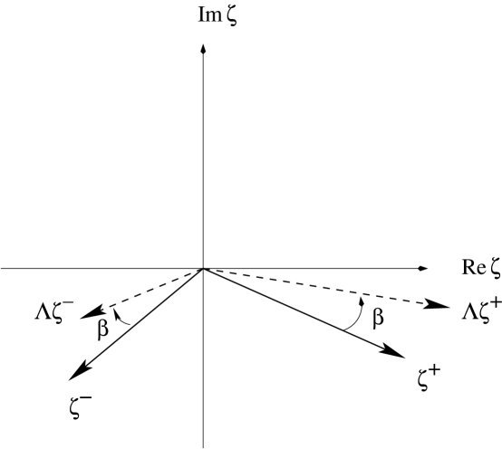
Figure 2: Under a complex O(1,1) boost with rapidity $\alpha+i\beta$ the null coordinates $\zeta^{\pm}$ are rotated in opposite directions. A one-parameter family of transformations can be constructed by considering two monotonous functions $(\alpha(t),\beta(t))$ with $0\leq t\leq 1$ interpolating between (0,0) and $(\alpha,\beta)$ such that all the transformed points lie in the lower half-plane and therefore belong to $\mathfrak{T}_{1}$.

As shown in Fig. 2 the effect of a complex transformation is to rotate the null coordinates $\zeta^{\pm}$ by an angle $\beta$ in opposite directions (at the same time than rescaling them by $e^{\alpha}$). Therefore, if the initial and the final points lie in $\mathfrak{T}_{1}$, i.e. in the lower half plane, there is always a family of transformations which interpolate between the two and such that the transformed

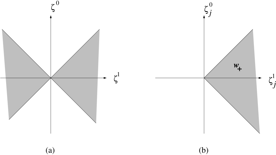
Figure 3: Set of Jost points: (a) for $\mathfrak{T}_{1}^{\prime}$; (b) for $\mathfrak{T}_{n-1}^{\prime}$ with $n>2$ the set of Jost points is the product of $n-1$ copies of the wedge $w_{+}$.

points always have negative imaginary parts. The extension to $\mathfrak{T}_{n-1}$ with $n>2$ is straightforward.

This proves that the Wightman functions can be analytically continued to the extended tube $\mathfrak{T}_{n-1}^{\prime}$. Unlike the tube $\mathfrak{T}_{n-1}$, the extended tube does contain real points. By analogy with the standard case, we call these real points Jost points. Actually, the analog of a theorem proved by Jost [17] holds in this case, namely, that a point $(\zeta_{1},\ldots,\zeta_{n-1})\in\mathfrak{T}_{n-1}^{\prime}$ is real if and only if, any combination of the form

$$\sum_{j=1}^{n-1}\lambda_{j}\zeta_{j},\,\,\,\,\mbox{with}\,\,\,\,\lambda_{j}\geq 0\,\,\,\,\mbox{and}\,\,\,\,\sum_{j=1}^{n-1}\lambda_{j}^{2}>0$$ (4.6)

lies outside the light wedge,

$$\left(\sum_{j=1}^{n-1}\lambda_{j}\zeta_{j}^{0}\right)^{2}-\left(\sum_{j=1}^{n-1}\lambda_{j}\zeta_{j}^{1}\right)^{2}<0.$$ (4.7)

Although the condition (4.7) is weaker than the ordinary one, the Jost points still form a real neighborhood in the extended tube on which the “edge of the wedge” theorem can be applied. For $\mathfrak{T}_{1}^{\prime}$ the set of Jost points is the shadowed region depicted in Fig. 3a. They are formed by the wedge $(\zeta_{e})^{2}<0$. On the other hand, for $\mathfrak{T}_{n-1}$ with $n>2$ the set of Jost points is given by $w_{+}^{n-1}$, where $w_{+}$ is the wedge defined by $(\zeta_{e})^{2}<0$ and $\zeta^{1}>0$, as shown in Fig. 3b.

4.2 The proof of the theorem

We are ready now to proceed to demonstrate the CPT theorem. The main difference with the standard proof lies in the fact analytic continuation is performed only in the electric components of the coordinates and only invariance under O(1,1)$\times$SO(2) is assumed. However, the existence of this unbroken subgroup of the Lorentz group is enough to ensure that the PT transformation can be connected to the identity by a family of complex boosts.

In terms of the Wightman functions, the CPT theorem for a neutral scalar field $\phi(x)$ states that

$$\langle\Omega|\phi(x_{1})\ldots\phi(x_{n})|\Omega\rangle=\langle\Omega|\phi(-x_{n})\ldots\phi(-x_{1})|\Omega\rangle.$$ (4.8)

This identity is equivalent to the following one for the analytically continued Wightman function into the extended tube $\mathfrak{T}_{n-1}^{\prime}$ (cf. [17, 18])

$$\mathscr{W}_{n}(\zeta_{1},\ldots,\zeta_{n-1})=\mathscr{W}_{n}(\zeta_{n-1},\ldots,\zeta_{1}),\hskip 28.45274pt(\zeta_{1},\ldots,\zeta_{n-1})\in\mathfrak{T}_{n-1}^{\prime}.$$ (4.9)

We prove now that Eq. (4.8), and therefore the CPT theorem, is equivalent to the condition of adapted weak local commutativity

$$\langle\Omega|\phi(x_{1})\ldots\phi(x_{n})|\Omega\rangle=\langle\Omega|\phi(x_{n})\ldots\phi(x_{1})|\Omega\rangle\hskip 28.45274pt$$ (4.10)

with $(x_{1}-x_{2},\ldots,x_{n-1}-x_{n})$ a Jost point. Since Jost points are real and lie outside the light wedge, the condition (4.10) follows from the adapted postulate of microcausality introduced in Section 3.3.

We begin by rewriting the condition (4.10) as an identity between Wightman functions at Jost points

$$\mathscr{W}_{n}(\zeta_{1},\ldots,\zeta_{n-1})=\mathscr{W}_{n}(-\zeta_{n-1},\ldots,-\zeta_{1}).$$ (4.11)

Since this identity holds at Jost points, and these form a real neighborhood of the domain of analyticity of the Wightman functions, one concludes, using the “edge of the wedge” theorem [18], that Eq. (4.10) is valid in the whole extended tube $\mathfrak{T}_{n-1}^{\prime}$.

As it was discussed in Section 2, the inversion of the four space-time coordinates is the product of the transformation $I_{\rm st}\in\mathfrak{L}_{+}(\mathbb{C})$ [see Eq. (3.15)] and a SO(2)-rotation of $\pi$. Therefore, the transformation $I_{\rm st}$ is a real transformation belonging to O(1,1)$\times$SO(2). Applying the covariance of the Wightman functions under $\mathfrak{L}_{+}(\mathbb{C})\times\mbox{SO(2)}$ we can write

$$\mathscr{W}_{n}(\zeta_{1},\ldots,\zeta_{n-1})=\mathscr{W}_{n}(I_{\rm st}\zeta_{n-1},\ldots,I_{\rm st}\zeta_{1})=\mathscr{W}_{n}(\zeta_{n-1},\ldots,\zeta_{1}).$$ (4.12)

This identity is true for all points in $\mathfrak{T}_{n-1}^{\prime}$ and therefore it also holds in the tube $\mathfrak{T}_{n-1}$. Since the Wightman function $\langle\Omega|\phi(x_{1})\ldots\phi(x_{n})|\Omega\rangle$ are the boundary values of the analytic function $\mathscr{W}_{n}(\zeta_{1},\ldots,\zeta_{n-1})$ defined in the tube, this proves the CPT theorem (4.8) for a neutral scalar field

The reverse is also easily proved. Indeed, if Eq. (4.9) holds in the extended tube using again the covariance of the Wightman functions under $\mathfrak{L}_{+}(\mathbb{C})\times\mbox{SO(2)}$ we conclude that Eq. (4.11) holds also at all points in the extended tube. Therefore the relation is satisfied in particular at the Jost points and we recover the adapted weak local commutativity condition (4.10).

We have proved that the CPT theorem holds in noncommutative quantum field theories satisfying the adapted axioms, in particular the postulate of weak local commutativity. As discussed in Section 3.2 the vacuum expectation value of the commutator of two scalar fields does not vanish for those noncommutative theories containing states in tachyonic representations of $\mathfrak{P}$. This implies that for this type of theories the adapted postulate of microcausality does not hold in general. This is for example the case of theories with time-space noncommutativity ($\theta_{e}\neq 0$) [30]. In Refs. [20, 23] it was argued that the CPT theorem is also satisfied in these theories, based on the transformation properties of the different terms in the classical action. What we see is that even if CPT is a symmetry at tree level, the full quantum theory is not necessarily invariant.

4.3 Remarks on spin-statistics

If we consider representations of SO(1,1)$\times$ SO(2) induced from string theory, they are reductions of representations of SO(1,3). For them it is easy to extend the above proof of the CPT theorem

$$\langle\Omega|\Phi_{1}(x_{1})\ldots\Phi_{n}(x_{n})|\Omega\rangle=(-1)^{J}i^{F}\langle\Omega|\Phi_{n}(-x_{n})\ldots\Phi_{1}(-x_{1})|\Omega\rangle$$ (4.13)

where $F$ is the number of fermionic fields (which has to be even) and $J$ is the number of undotted indices that results when the SO(1,1)$\times$SO(2) representations are written in terms of representations of SO(1,3).

If instead one wants to consider representations of SO(1,1)$\times$SO(2) that do not follow from restrictions of those of SO(1,3), the structure of the phases is more delicate. The kinetic term for the fields will generically be very different from the standard four-dimensional case, and although the proof of CPT can be adapted to this case, the spin-statistics connection generically will fail.

For fully relativistic field theories, the spin-statistics theorem follow from the phases appearing in the CPT theorem Eq. (4.13). In the noncommutative case there are conceptual issues indicating that any spin-statistics theorem will be more difficult to come by. In the standard case, and for massive theories, the little group contains SO(3), a non-abelian group, which guarantees that the internal spin $s$ of the physical states will be quantized according to $s\in\mathbb{Z}$ for bosons and $s\in\mathbb{Z}+{1\over 2}$ for fermions. Thus, proving the spin-statistics connection requires among other things to show that their interpolating fields satisfy microcausality with commutators or anticommutators respectively. In the general noncommutative case these arguments fail, states with arbitrary helicity can be constructed, and it would not be surprising to find anyonic (or more exotic) behavior. For theories whose field content descent from string theory via the Seiberg-Witten limit one expects that the standard arguments for the spin-statistic theorem can be adapted to the noncommutative case. The general case, however, remains to be elucidated.

5 Additional issues

In theories with space-space noncommutativity, violations of CPT invariance can still appear for two reasons. The first one is the appearance of tachyonic states in the spectrum which would spoil adapted weak local commutativity. The second thing that can go wrong with the proof is that the Wightman functions do not define tempered distributions on the space $\mathscr{S}[(\mathbb{R}^{1,3})^{n}]$. This is the case, for example, if hard infrared singularities appear in the correlation functions induced by ultraviolet quadratic divergences via UV/IR mixing [14]. If this happens, the analytic continuation of the Wightman functions into the (extended) tube might not be possible.

The two problems appear in the case of pure noncommutative QED with space-space noncommutativity ($\theta_{e}=0$, $\theta_{m}\equiv\theta$.), where the one-loop corrected dispersion relation presents a tachyonic instability at low energies [40]

$$\omega(\vec{p})^{2}=\vec{p}^{\,2}-{2g^{2}\over\pi^{2}\,p\circ p}.$$ (5.1)

At the same time, the correlation functions are afflicted with infrared singularities derived from uncancelled quadratic ultraviolet divergences. A regularization of these divergences by considering $\mathcal{N}=1$, U(1)_⋆ gauge theory softly broken to $\mathcal{N}=0$ does not eliminate the problem of the tachyonic states, since a negative, $\theta$-independent squared mass for the photon is generated $m_{\rm photon}^{2}=-g^{2}M^{2}/(2\pi^{2})$, with $M$ the soft breaking mass of the gaugino [43].

To overcome these problems, we study U(1)_⋆, $\mathcal{N}=4$ noncommutative gauge theory softly broken to $\mathcal{N}=0$ by mass terms for the fermions and the scalars [44, 45]. This soft-breaking of supersymmetry introduces at most logarithmic divergences in higher order amplitudes that do not destroy the tempered nature of the correlation functions [46].

Before entering into the details of how this theory renders a non-tachyonic dispersion relation for the photon at low energies, it is convenient to briefly discuss some aspects of the regularization of noncommutative gauge theories. In the usual case, the most popular regularization procedure is dimensional regularization, which straightforwardly extends to the noncommutative case. However, in studying the Wilsonian low-energy effective action of noncommutative gauge theories, it would be convenient to introduce a “sharp” cutoff in momentum space $\Lambda$. In this case the origin of the difficulties with UV/IR mixing are relatively easy to understand: since the elementary objects are not particles but rigid dipoles of length $|\theta^{\mu\nu}p_{\nu}|$, a ultraviolet cutoff in momenta $\Lambda$ induces an infrared cutoff $1/(\theta\Lambda)$, the inverse of the maximal dipole length. Since at distances much larger than the length of the maximal dipole the elementary objects behave again like particles, the commutative theory has to be recovered at momenta $|\vec{p}|\ll 1/(\theta\Lambda)$ and at the same time Lorentz invariance is restored.

In the case of gauge theories, however, there is no obvious sharp momentum cutoff (apart from the lattice) compatible with gauge invariance and the previous picture is not fully realized. Using dimensional regularizaton, for example, the whole region $0\leq|\vec{p}|\leq 1/(\theta\Lambda)$ disappears. On the other hand, using a cutoff in the Schwinger parameter leads to violations of gauge invariance. This contrast with the case, for example, of $\phi^{\star 3}$-theory in six-dimensions, where the picture outlined above is realized.

In order to avoid these problems we could use an “intermediate” cutoff: we use dimensional regularization to regularize the integrals along the directions orthogonal to the space-like vector $\tilde{p}^{\mu}\equiv\theta^{\mu\nu}p_{\nu}$ (with $p_{\mu}$ the external momentum) while for the computation of the last integral along the direction of $\tilde{p}^{\mu}$ we use a Schwinger cutoff. This procedure works for generic external momenta, i.e. $p\neq 0$, $\tilde{p}\neq 0$. Its advantage lies in the fact that it exposes some of the features of the “sharp” cutoff explained above while preserving gauge invariance.

We proceed now to compute the one-loop effective action $\Gamma(\mathcal{A})_{\rm eff}$ for gauge field for a $\mathcal{N}=4$, U(1) noncommutative gauge theory softly broken to $\mathcal{N}=0$ by mass terms for the fermions and scalars in the theory

$$\Gamma(\mathcal{A})_{\rm eff} = -{1\over 2}\log\det\Delta_{\rm gauge}+\log\det\Delta_{\rm ghosts}+{n_{f}\over 2}\log\det\Delta_{f}-{n_{s}\over 2}\log\det\Delta_{s}$$ (5.2)

$$\equiv {1\over 2}\int{d^{4}p\over(2\pi)^{4}}\mathcal{A}^{\mu}(p)\Pi_{\mu\nu}(p)\mathcal{A}^{\mu}(-p)+\mathcal{O}(\mathcal{A}^{3}),$$

where $n_{f}$ and $n_{s}$ denote respectively the number of Weyl fermions and real scalars in the theory. For $\mathcal{N}=1$ noncommutative U(1) supersymmetric Yang-Mills we have $n_{f}=1$, $n_{s}=0$, whereas for $\mathcal{N}=2$ one has $n_{f}=2$, $n_{s}=2$ and $n_{f}=4$, $n_{s}=6$ for $\mathcal{N}=4$.

Following [45], we use the background field method and work in Euclidean space. The photon self-energy can be written as the sum of the planar and the nonplanar contribution as [47]

$$\Pi_{\mu\nu}(p)=\Pi_{\mu\nu}(p,\ell=0)-\Pi_{\mu\nu}(p,\ell=\tilde{p})$$ (5.3)

with

$$\Pi_{\mu\nu}(p,\ell) = 2\sum_{j}\alpha_{j}\int{d^{4}k\over(2\pi)^{4}}\left\{d(j)\left[{(2k+p)_{\mu}(2k+p)_{\nu}\over(k^{2}+m_{j}^{2})[(k+p)^{2}+m_{j}^{2}]}-{2\delta_{\mu\nu}\over k^{2}+m_{j}^{2}}\right]\right.$$ (5.4)

$$+ \left.4C(j){p^{2}\delta_{\mu\nu}-p_{\mu}p_{\nu}\over(k^{2}+m_{j}^{2})[(k+p)^{2}+m_{j}^{2}]}\right\}e^{ik\cdot\ell}.$$

The sum is over all states running in the loop (gauge fields, ghosts, fermions and scalars). The constant $\alpha(j)$, $d(j)$ and $C(j)$, as well as the masses for the different fields, are given in the following table:

$$\begin{array}[]{|c|c|c|c|c|}\hline\cr&&&&\\ j&{\rm ghost}&\mbox{real scalar}&\mbox{Weyl fermion}&\mbox{gauge field}\\ &&&&\\ \hline\cr&&&&\\ \alpha_{j}&1&-{1\over 2}&{1\over 2}&-{1\over 2}\\ &&&&\\ d(j)&1&1&2&4\\ &&&&\\ C(j)&0&0&{1\over 2}&2\\ &&&&\\ m_{j}&0&M_{s}&M_{f}&0\\ &&&&\\ \hline\cr\end{array}$$

In theories with unbroken (or softly broken) supersymmetry the condition ${\rm Str\,}\mathbf{1}=0$ translates into

$$\sum_{j}\alpha_{j}d(j)=n_{f}-{n_{s}\over 2}-1=0$$ (5.6)

whereas in theories with $\mathcal{N}=4$ (or $\mathcal{N}=2$ with two hypermultiplets) we have the additional identity

$$\sum_{j}\alpha_{j}C(j)\equiv{n_{f}\over 4}-1=0.$$ (5.7)

For supersymmetric theories (5.6) guarantees the vanishing of the terms proportional to $\tilde{p}_{\mu}\tilde{p}_{\nu}$ in the vacuum polarization, and the dispersion relation of the photon is not modified. In the particular case of noncommutative gauge theories with $\mathcal{N}=4$ unbroken supersymmetry the identity (5.7) further implies that $\Pi_{\mu\nu}(p)=0$. If soft breaking masses are included these cancellations are not complete but, as we will see below, they are enough to tame the problems arising from UV/IR mixing.

In evaluating (5.4) we come back to the issue of regularization in more detail. There are various ways to regulate the planar diagram contribution $(\ell=0)$, but few for the non-planar part ($\ell=\tilde{p}$) preserving gauge invariance. Physically, when working with the low-energy Wilsonian effective action it is convenient to introduce some kind of sharp cutoff $\Lambda$ which eliminates the physics at scales $E>\Lambda$. In theories without gauge symmetry, and at one loop, this can be achieved by exponentiation of the propagators using Schwinger parameters and modifying their integration measure. For instance, for two propagators the procedure amounts to the prescription

$${1\over(p_{1}^{2}+m_{1}^{2})(p_{2}^{2}+m_{2}^{2})} = \int_{0}^{\infty}d\alpha_{1}d\alpha_{2}\exp\left[-\alpha_{1}(p_{1}^{2}+m_{1}^{2})-\alpha_{1}(p_{2}^{2}+m_{2}^{2})\right]$$

$$\longrightarrow\hskip 8.5359pt \int_{0}^{\infty}d\alpha_{1}d\alpha_{2}\exp\left[-\alpha_{1}(p_{1}^{2}+m_{1}^{2})-\alpha_{1}(p_{2}^{2}+m_{2}^{2})-{1\over 4\Lambda^{2}(\alpha_{1}+\alpha_{2})}\right].$$

Proceeding along these lines, Eqs. (5.3) and (5.4) become after some computation

$$\Pi_{\mu\nu}(p) = {1\over 4\pi^{2}}\left(p^{2}\delta_{\mu\nu}-p_{\mu}p_{\nu}\right)$$ (5.9)

$$\,\,\times\,\,\sum_{j}\alpha_{j}\int_{0}^{1}dx\,\left[4C(j)-(1-2x)^{2}d(j)\right]\left[K_{0}\left({\sqrt{\Delta_{j}}\over\Lambda}\right)-K_{0}\left({\sqrt{\Delta_{j}}\over\Lambda_{\rm eff}}\right)\right]$$

$$+ {1\over(4\pi)^{2}}\tilde{p}_{\mu}\tilde{p}_{\nu}\,\Lambda_{\rm eff}^{2}\sum_{j}\alpha_{j}d(j)\int_{0}^{1}dx\,\Delta_{j}K_{2}\left({\sqrt{\Delta_{j}}\over\Lambda_{\rm eff}}\right)$$

$$+ \delta_{\mu\nu}\left[\mbox{ gauge non-invariant term }\right],$$

where $\Delta_{j}=m_{j}^{2}+x(1-x)p^{2}$ and the effective cutoff is given by [14]

$${1\over\Lambda_{\rm eff}^{2}}={1\over\Lambda^{2}}+\tilde{p}^{2}$$ (5.10)

and we have expressed the integrals over Schwinger parameters in terms of modified Bessel functions of the second kind

$$K_{\nu}(\alpha z)={\alpha^{\nu}\over 2}\int_{0}^{\infty}{dt\over t^{\nu+1}}e^{-{z\over 2}\left(t+{\alpha^{2}\over t}\right)}.$$ (5.11)

Ignoring momentarily the gauge non-invariant term, the answer (5.9) is satisfactory in several ways. For fixed $\Lambda$, in the momentum region $|\vec{p}|<1/(\Lambda\theta)$ we recover Lorentz invariance and the standard dispersion relation for the photon. Also there is no ambiguity in taking the limit $\tilde{p}\rightarrow 0$. The big drawback, of course, is the lack of gauge invariance, due to the term proportional to $\delta_{\mu\nu}$. This term can only be subtracted by local counterterms for the planar diagram.

Had we used dimensional regularization, the answer would be given by the leading term of (5.9) in the limit $\Lambda\rightarrow\infty$, at fixed $\tilde{p}$,

$$K_{0}\left({\sqrt{\Delta_{j}}\over\Lambda}\right)\longrightarrow-{1\over 2}\log\left({\Delta_{j}\over 4\pi\mu^{2}}\right);\hskip 28.45274pt\Lambda_{\rm eff}\longrightarrow{1\over|\tilde{p}|}$$ (5.12)

and with the gauge non-invariant term absent (cf. [48]). In this limit the region $0<|\vec{p}|<1/(\Lambda\theta)$ disappears.

It is possible to imagine an intermediate regulator where the loop integrals are split into a three-dimensional part, which is evaluated using dimensional regularization in $3-\epsilon$ dimensions, and a fourth integral which is regularized using a Schwinger cutoff. In order to implement this regularization we consider for generic $p$ (i.e. $p\neq 0$, $\tilde{p}\neq 0$) an orthonormal frame ${\rm e}_{\hat{a}\mu}$ ($\hat{a}=1,\ldots,4$)

$${\rm e}_{\hat{1}\mu}={\tilde{p}_{\mu}\over|\tilde{p}|},\hskip 14.22636pt{\rm e}_{\hat{2}\mu}={p_{\mu}\over|p|}$$ (5.13)

and ${\rm e}_{\hat{3}\mu}$, ${\rm e}_{\hat{4}\mu}$ chosen so that ${\rm e}_{\hat{a}\mu}\cdot{\rm e}_{\hat{b}\nu}=\delta_{\hat{a}\hat{b}}$. In this case Eq. (5.4) can be split into an integral over $k_{\hat{1}}$, which is regulated using a Schwinger cutoff (physically, this corresponds to regulating the length of the dipoles running in the loop), and the remaining three-dimensional integral, which can be dealt with using dimensional regularization.

Implementing this “mixed” regulator we find a result for the polarization tensor which is not identical to (5.9), but in which the gauge non-invariant term is absent and the effective cutoff $\Lambda_{\rm eff}$ appearing in the third line of this equation is replaced by $(2\tilde{p}^{2}\Lambda_{\rm eff}^{2}-1)/\tilde{p}^{2}$. If we take the limit $\Lambda\rightarrow\infty$ with $\tilde{p}$ fixed, we recover the result of dimensional regularization, again with the identification $\Lambda^{2}\rightarrow 4\pi\mu^{2}$. The main problem with this procedure is that it is not clear whether it can be systematically extended to higher loops.

5.1 Softly broken $\mathcal{N}=4$, U(1)_⋆ gauge theory

Let us now focus on the case of $\mathcal{N}=4$, noncommutative U(1) gauge theory. Using dimensional regularization, the polarization tensor can be written as

$$\Pi_{\mu\nu}(p)=\Pi_{1}(p)(p^{2}\delta_{\mu\nu}-p_{\mu}p_{\nu})+\Pi_{2}(p){\tilde{p}_{\mu}\tilde{p}_{\nu}\over\tilde{p}^{2}},$$ (5.14)

where

$$\Pi_{1}(p) = {1\over 4\pi^{2}}\int_{0}^{1}dx\left\{\left[4-(1-2x)^{2}\right]\left[{1\over 2}\log\left({\Delta_{v}\over 4\pi\mu^{2}}\right)+K_{0}(\sqrt{\Delta_{v}}|\tilde{k}|)\right]\right.$$ (5.15)

$$- \left[1-(1-2x)^{2}\right]\sum_{f}\left[{1\over 2}\log\left({\Delta_{f}\over 4\pi\mu^{2}}\right)+K_{0}(\sqrt{\Delta_{f}}|\tilde{k}|)\right]$$

$$- \left.{1\over 2}(1-2x)^{2}\sum_{s}\left[{1\over 2}\log\left({\Delta_{s}\over 4\pi\mu^{2}}\right)+K_{0}(\sqrt{\Delta_{v}}|\tilde{k}|)\right]\right\}$$

and

$$\Pi_{2}(p) = -{1\over\pi^{2}}\int_{0}^{1}dx\,\left[\Delta_{v}K_{2}(\sqrt{\Delta_{v}}|\tilde{p}|)-\sum_{f}\Delta_{f}K_{2}(\sqrt{\Delta_{f}}|\tilde{p}|)\right.$$ (5.16)

$$+ \left.{1\over 2}\sum_{s}\Delta_{s}K_{2}(\sqrt{\Delta_{s}}|\tilde{p}|)\right]$$

The subindices $v$, $f$ and $s$ indicate respectively the contributions of the vector-ghost system, fermions and scalars, and

$$\Delta_{v}=x(1-x)p^{2},\hskip 28.45274pt\Delta_{f}=m_{f}^{2}+x(1-x)p^{2},\hskip 28.45274pt\Delta_{s}=m_{s}^{2}+x(1-x)p^{2}.$$ (5.17)

The Wilsonian effective coupling constant at momentum $p$ is determined by $\Pi_{1}(p)$, namely

$${1\over g(p)^{2}}-{1\over g_{0}^{2}}=\Pi_{1}(p).$$ (5.18)

For values of the momenta larger that the noncommutative scale, $p\gg 1/\sqrt{\theta}$, the Bessel functions decay exponentially and only the logarithms in (5.15) contribute, reproducing the standard $\beta$-function of the theory

$$\Pi_{1}(p)\simeq{1\over 8\pi^{2}}\left({11\over 3}-{2\over 3}n_{f}-{1\over 6}n_{s}\right)\log\left({p^{2}\over 4\pi\mu^{2}}\right),\hskip 28.45274pt|p|\gg{1\over\sqrt{\theta}}.$$ (5.19)

If we have a field content corresponding to softly broken $\mathcal{N}=4$ U(1) theory, a $\mathcal{N}=1$ vector multiplet and three chiral multiplets in the adjoint representation, the $\beta$-function vanishes. In fact the theory is believed to be ultraviolet finite [49].

Before considering the modifications that arise from the introduction of the soft breaking masses, we consider the supersymmetric case where $M_{f}=M_{s}=0$. In this case there is an interesting phenomenon associated with UV/IR mixing. If we consider the region of small momenta $p\ll 1/\sqrt{\theta}$ the Bessel function can be approximated by its leading logarithm behavior and therefore we have

$$-{1\over 2}\log\left({\Delta\over 4\pi\mu^{2}}\right)-K_{0}(\sqrt{\Delta}|\tilde{p}|)\simeq{1\over 2}\log(4\pi\mu^{2}\tilde{p}^{2})$$ (5.20)

Therefore, in this limit we find for $\Pi_{1}(p)$

$$\Pi_{1}(p)\simeq{1\over 8\pi^{2}}\left(-{11\over 3}+{2\over 3}n_{f}+{1\over 6}n_{s}\right)\log(4\pi\mu^{2}\tilde{p}^{2}),\hskip 28.45274pt|p|\ll{1\over\sqrt{\theta}}$$ (5.21)

Comparing Eqs. (5.19) with (5.21) we find that the running of the coupling constant in the infrared is completely similar to the one in the ultraviolet, except for a change in the sign. The different sign indicates that, for theories with a negative $\beta$-function, the theory becomes weakly coupled again at low energies. This kind of duality in momenta, $p\leftrightarrow 1/\tilde{p}$, is a reflection of the mixing of high and low energy scales characteristic of noncommutative field theories.

We next proceed to include the soft breaking masses for the fermions and the scalars. In particular, we will consider the $\mathcal{N}=4$ theory in the region of momenta $|p|\ll m_{j}<1/\sqrt{\theta}$. In this case, $\Pi_{1}(p)$ can be written as

$$\Pi_{1}(p)={1\over 8\pi^{2}}\left(-{11\over 3}\right)\log\left({M_{\rm eff}^{2}\tilde{p}^{2}}\right)+\mbox{exponentially vanishing terms}$$ (5.22)

where the effective mass is given by

$$M_{\rm eff}=\left(\prod_{f=1}^{4}M_{f}^{2}\prod_{s=1}^{6}M_{s}^{1\over 2}\right)^{1\over 11},$$ (5.23)

again leading to a weakly coupled theory in the infrared. Hence from this point of view the Wilsonian effective action is well defined. At low-energies we recover asymptotically an effective theory of a photon whose coupling constant vanishes in the infrared. These conclusions hold as long as there are no tachyons in the spectrum, which among other things destroy the possibility of having a weak version of local commutativity needed in the proof of the CPT theorem, as already discussed in Section 4.

As we mentioned, pure $\mathcal{N}=1$, U(1)_⋆ with a mass term for the photino leads to a low-energy tachyon pole for the photon [43]. In our case, since we can also play with the scalar masses, it is possible to choose values of the soft breaking masses for the fermions and the scalar in such a way that we avoid this problem. To understand the photon dispersion relation we need to compute the full propagator following from (5.14).

In order to find the poles of the full propagator we should resum the two-point 1PI diagrams. The structure of (5.14) suggest the introduction of the non-orthogonal projectors

$$P_{\mu\nu} = \left(\delta_{\mu\nu}-{p_{\mu}p_{\nu}\over p^{2}}\right),$$

$$Q_{\mu\nu} = {\tilde{p}_{\mu}\tilde{p}_{\nu}\over\tilde{p}^{2}}$$ (5.24)

which satisfy (in matrix notation)

$$\mathbf{P}^{n}=\mathbf{P},\hskip 28.45274pt\mathbf{Q}^{n}=\mathbf{Q},\hskip 28.45274pt\mathbf{PQ}=\mathbf{QP}=\mathbf{Q}$$ (5.25)

so the polarization tensor in Eq. (5.14) can be written

$$\mathbf{\Pi}(p)=p^{2}\Pi_{1}(p)\mathbf{P}+\Pi_{2}(p)\mathbf{Q}.$$ (5.26)

The full propagator can then be written as

$$G_{\mu\nu}(p)={ig_{0}^{2}\over p^{2}}\left[\mathbf{1}+{-g_{0}^{2}\over p^{2}}\mathbf{\Pi}(p)+\left({-g_{0}^{2}\over p^{2}}\right)^{2}\mathbf{\Pi}(p)^{2}+\ldots\right]_{\mu\nu}.$$ (5.27)

In order to resum the series, we use Eq. (5.25) to write

$$\mathbf{\Pi}(p)^{n}=\left[p^{2}\Pi_{1}(p)\right]^{n}\mathbf{P}+\left\{\left[p^{2}\Pi_{1}(p)+\Pi_{2}(p)\right]^{n}-\left[p^{2}\Pi_{1}(p)\right]^{n}\right\}\mathbf{Q}$$ (5.28)

so the full propagator is given by

$$G_{\mu\nu}(p) = {ig_{0}^{2}p_{\mu}p_{\nu}\over p^{2}}+{ig_{0}^{2}\over p^{2}[1+g_{0}^{2}\Pi_{1}(p)]}\left(\delta_{\mu\nu}-{p_{\mu}p_{\nu}\over p^{2}}\right)$$ (5.29)

$$+ \left\{{ig_{0}^{2}\over p^{2}\left[1+g_{0}^{2}\Pi_{1}(p)\right]+g_{0}^{2}\Pi_{2}(p)}-{ig_{0}^{2}\over p^{2}[1+g_{0}^{2}\Pi_{1}(p)]}\right\}{\tilde{p}_{\mu}\tilde{p}_{\nu}\over\tilde{p}^{2}}.$$

Therefore, from Eq. (5.29) we find that the pole conditions are

$$p^{2}\left[{1\over g_{0}^{2}}+\Pi_{1}(p)\right] = 0$$ (5.30)

and

$$p^{2}\left[{1\over g_{0}^{2}}+\Pi_{1}(p)\right]+\Pi_{2}(p) = 0.$$ (5.31)

To obtain the dispersion relations for physical particles we have to rotate to Minkowski space by taking $p^{2}\rightarrow-p^{2}$ and $\tilde{p}^{2}\rightarrow p\circ p$. Equation (5.30) implies that one of the polarizations of the photon corresponds to a massless degree of freedom. On the other hand, Eq. (5.31) is associated to a photon whose polarization is proportional to ${\tilde{p}}^{\mu}$. To determine the pole in this case we need the low energy behavior of $\Pi_{2}(p)$. From (5.16), and using the small argument expansion of $K_{2}(z)$, we obtain after simple manipulations

$$\Pi_{2}(p) = {1\over\pi^{2}}\left(-1+n_{f}-{n_{s}\over 2}\right)\left({2\over{\tilde{p}}^{2}}-{p^{2}\over 12}\right)-{1\over 2\pi^{2}}\left(\sum_{f}M_{f}^{2}-{1\over 2}\sum_{s}M_{s}^{2}\right)+\ldots$$ (5.32)

In $\mathcal{N}=4$ noncommutative super Yang-Mills, we have $-1+n_{f}+{n_{s}\over 2}=0$. Hence to avoid tachyons we need to satisfy

$$\sum_{f}M_{f}^{2}-{1\over 2}\sum_{s}M_{s}^{2}\leq 0$$ (5.33)

which implies ${\rm Str\,}M^{2}\geq 0$. This condition guarantees, to this order in perturbation theory, that the spectrum is free of tachyons. Although when the equality in (5.33) is satisfied we recover formally a massless photon at zero momentum, the function $\Pi_{2}(p)$ is negative in a neighborhood of $\tilde{p}=0$. Therefore, in order to avoid problems the soft-breaking masses has to be tuned so the photon has a positive mass squared at zero momentum.

Figure 4: Dispersion relation $p^{2}$ versus $t$.

In Fig. 5 we have plotted the dispersion relation by solving (5.31) as an implicit equation for $p^{2}\equiv s-t$ and $t\equiv p\circ p/\theta^{2}$, when the strict inequality in (5.33) is satisfied. The positive intercept in the curve implies that the photons with this polarization become massive, something that phenomenologically is a disaster. The current bound on the photon mass is $m_{\gamma}<2\times 10^{-16}$ eV [50], hence to satisfy it one would have to do a rather non-trivial fine tuning in the expansion of $\Pi_{2}(p)$. However, even if this is achieved, the dispersion relation is likely to produce birefringence, i.e. the speed of light would be different for polarizations along the commutative and noncommutative directions. This effect would come from the terms in $\Pi_{2}(p)$ quadratic in $p_{\mu}$ and ${\tilde{p}}_{\mu}$. Again in this case the bounds are very restrictive. Another very strict bound can also be extracted by looking at the departures from the black body radiation that a massive polarization for the photon produces.

It is clear that the phenomenological prospects for this theory are rather slim. The main purpose to study it was to show that it is possible to construct a noncommutative field theory satisfying the adapted axioms introduced in Section 3.3. At least in perturbation, theory the correlation functions calculated are tempered distributions, the theory is well defined both in the ultraviolet and the infrared, and the renormalization procedure and the computation of the Wilsonian effective action will not be afflicted by hard infrared divergences that would lead to Wightman functions with non-tempered singularities. This is for instance the reason why massless scalar fields in two-dimensions do not exist [51].

Before closing this section, we make some remarks about the resulting dispersion relations using other regularizations procedures mentioned above involving a sharp cutoff. Modulo the problems already pointed out, in this case we find that for the photons with polarizations along $\tilde{p}^{\mu}$ the usual dispersion relation $p^{2}=0$ is recovered for both low and high noncommutative momenta with respect to the noncommutative scale $1/\sqrt{\theta}$. Around this noncommutative scale, however, one finds a region where the group velocity of waves packets becomes superluminal. This situation is highly reminiscent of the situation described in [52] for noncommutative field theories at finite temperature. This is however not so surprising if one keeps in mind that in thermal noncommutative field theory the temperature plays the role of a “sharp” cutoff. Indeed, at fixed $T$ a noncommutative U(1)_⋆ gauge theory has a smooth infrared (and commutative) limit [53] due to the fact that the Boltzmann factors in the temperature-dependent part of the loop integrals cut off any physics above the scale $T$, thus regularizing the UV/IR mixing of noncommutative gauge theories.

Although we have concentrated only on the one-loop vacuum polarization for the photon, we expect the same conclusions to apply to higher orders, and also to higher point functions. The theory considered is believed to be finite in the ultraviolet, and once the possibility of tachyon poles is allayed, the correlation functions for the theory should be described in terms of tempered distributions, and the low-energy Wilsonian effective action should also be well defined. Nevertheless, the constraint between the soft-breaking masses (5.33) is very likely to be modified by the inclusion of higher loop corrections.

6 Concluding remarks

In this paper we have studied some general properties of noncommutative quantum field theories. An axiomatic formulation can be achieved by modifying the standard Wightman axioms using as guiding principles i) the breaking of Lorentz symmetry down to the subgroup O(1,1)$\times$SO(2), and ii) the relaxation of local commutativity to make it compatible with the causal structure of the theory, given by the light-wedge associated with the O(1,1) factor of the kinematical symmetry group.

These axioms are enough to demonstrate the CPT theorem. Indeed, this theorem holds for these theories for reasons not very different from the ones behind the CPT theorem for commutative theories. The transformation PT is in the connected component of the identity in the group that result from the complexification of the O(1,1) subgroup of the symmetry group. This, together with the tempered character of the distributions defined by the Wightman functions, allows to use results like the “edge of the wedge” theorem to show that the Wightman functions and their CPT-transforms coincide.

The main source of difficulties in formulating noncommutative field theories which satisfy the adapted axioms is UV/IR mixing. The existence of hard infrared singularities in the non-planar sector of the theory, induced by uncancelled quadratic ultraviolet divergences, can result in two kinds of problems: they can destroy the tempered nature of the Wightman functions and/or they can introduce tachyonic states in the spectrum, so the modified postulate of local commutativity is not preserved.

In this sense, we have also shown how it is possible to construct noncommutative field theories which, at least in perturbation theory, are compatible with the adapted axioms. Noncommutative QED is an example of a theory which does not satisfy the axioms due to the emergence of tachyons due to UV/IR mixing. This mixing of scales can be tamed by completing noncommutative QED to $\mathcal{N}=4$ U(1)_⋆ super Yang-Mills and breaking supersymmetry softly by introducing masses for the scalar and fermion fields. This eliminate the quadratic divergences and, if the soft-breaking masses are tuned, remove tachyonic instabilities at low momentum. Similar arguments will apply to higher orders in perturbation theory and higher point functions since the underlying theory is finite ${\cal N}=4$ noncommutative QED. We have also shown that in this context the U(1) theory obtained is a phenomenological disaster. There are other approaches to phenomenology in noncommutative field theories (see for instance [54]), where one first expands the action up to a certain order in $\theta$ and then quantizes the theory obtained. We know, however, that generally the two procedures do not necessarily generate the same results due to the UV/IR mixing.

References

-
[1]
A. Connes,
Noncommutative Geometry,
Academic Press 1994.
J. Madore, An Introduction to Noncommutative Differential Geometry and its Applications, Cambridge 1995.
G. Landi, An Introduction to Noncommutative Spaces and Their Geometries, Springer 1997 [arXiv:hep-th/9701078].
J. M. Gracia-Bondía, J. C. Varilly and H. Figueroa, Elements Of Noncommutative Geometry, Birkhäuser 2001. -
[2]
K. von Klitzing, G. Dorda and M. Pepper,
New Method For High-Accuracy Determination Of The Fine-Structure
Constant Based
On Quantized Hall Resistance,
Phys. Rev. Lett. 45 (1980) 494.
R. B. Laughlin, Anomalous Quantum Hall Effect: An Incompressible Quantum Fluid With Fractionally Charged Excitations, Phys. Rev. Lett. 50 (1983) 1395.
R. B. Laughlin, Quantized motion of three two-dimensional electrons in a strong magnetic field, Phys. Rev. B27 (1983) 3383. - [3] Z.F. Ezawa, Quantum Hall Effects. Field Theoretical Approach and Related Topics, World Scientific 2000.
-
[4]
J. Bellissard, D. R. Grempel, F. Martinelli and E. Scoppola,
Localization of electrons with spin-orbit or magnetic interactions in a
two-dimensional disordered crystal, Phys. Rev. B33 (1986) 641.
J. Bellissard, A. van Elst and H. Schulz-Baldes, The Noncommutative Geometry of the Quantum Hall Effect, arXiv:cond-mat/9411052.
L. Susskind, The quantum Hall fluid and non-commutative Chern Simons theory, arXiv:hep-th/0101029.
A. P. Polychronakos, Quantum Hall states as matrix Chern-Simons theory, J. High Energy Phys. 04 (2001) 011 [arXiv:hep-th/0103013].
J. L. F. Barbón and A. Paredes, Noncommutative field theory and the dynamics of quantum Hall fluids, Int. J. Mod. Phys. A17 (2002) 3589 [arXiv:hep-th/0112185]. - [5] A. Connes and J. Lott, Particle Models And Noncommutative Geometry, Nucl. Phys. Proc. Suppl. 18B (1991) 29.
- [6] C. P. Martín, J. M. Gracia-Bondía and J. C. Varilly, The standard model as a noncommutative geometry: The low-energy regime, Phys. Rept. 294 (1998) 363 [arXiv:hep-th/9605001].
- [7] E. Witten, Noncommutative Geometry And String Field Theory, Nucl. Phys. B 268 (1986) 253.
-
[8]
A. Connes, M. R. Douglas and A. Schwarz,