DAMTP-2003-03.

Abstract

Using an effective field theory approach, we address the effects on the gauge couplings of one and two additional compact dimensions in the presence of a constant background (gauge) field. Such background fields are a generic presence in models with extra dimensions and can be employed for gauge symmetry breaking mechanisms in the context of 4D N=1 supersymmetric models. The structure of the ultraviolet (UV) and infrared (IR) divergences that the gauge couplings develop in the presence of Wilson line vev’s is investigated. One-loop radiative corrections to the gauge couplings due to overlapping effects of the compact dimensions and Wilson line vev’s are computed for generic 4D N=1 models. Values of Wilson lines vev’s corresponding to points (in the “moduli” space) of enhanced gauge symmetry cannot be smoothly reached perturbatively from those corresponding to the broken phase. The one-loop corrections are compared to their (heterotic) string counterpart in the “field theory” limit $\alpha^{\prime}\rightarrow 0$ to show remarkably similar results when no massless states are present in a Kaluza-Klein tower. An additional correction to the gauge coupling exists in the effective field theory approach when for specific Wilson lines vev’s massless Kaluza-Klein states are present. This correction is not recoverable by the limit $\alpha^{\prime}\!\rightarrow\!0$ of the (infrared regularised) string because the infrared regularisation limit and the limit $\alpha^{\prime}\!\rightarrow\!0$ of the string result do not commute.

1 Introduction

The phenomenological and theoretical implications of the physics of “large” extra dimensions has recently attracted an increased research interest in the context of effective field theory approaches. String theory is ultimately thought to provide a complete and fully consistent description of the high energy physics. Nevertheless, effective field theory (EFT) approaches are able to describe accurately many aspects of the physics of extra dimensions, without relying on the string picture.

In this work we adopt an effective field theory approach to investigate the corrections to the gauge couplings in 4D N=1 supersymmetric models with one and two extra dimensions, in the presence of a constant background gauge field. The extra dimensions may be compactified on manifolds or orbifolds thereof [1] providing the possibility to construct chiral models. The compactification chosen and the value of the background gauge field (so-called Wilson lines’ vev’s [2], [3]) have implications for the one-loop corrections to the 4D gauge couplings and for the amount of gauge symmetry present. The interplay of these two effects on the 4D gauge couplings will be discussed in this work for the class of models considered. Let us first present this problem in detail.

Additional compact dimensions can induce significant changes to the 4D gauge couplings. The one-loop corrected coupling in an orbifold compactification to a 4D N=1 supersymmetric model is

$$\frac{4\pi}{g^{2}_{i}(Q)}=\frac{4\pi}{g_{i}^{2}(M_{s})}+\frac{b_{i}}{2\pi}\ln\frac{M_{s}}{Q}+\tilde{\Omega}_{i}+\cdots,\qquad\quad\textrm{{\it i}: \, gauge \,\, group \,\, index.}$$ (1)

$Q$ is a low energy scale above the supersymmetry breaking scale, $M_{s}$ is the ultraviolet scale or in the case of string theory, the string scale. In the EFT approach $g_{i}(M_{s})$ is the tree level (“bare”) coupling while in the (heterotic) string $g_{i}(M_{s})$ is actually a gauge group independent function of the so-called $S$ and $T$ moduli, invariant under $SL(2,Z)_{T}\!\times\!SL(2,Z)_{U}\!\times\!Z_{2}^{T\leftrightarrow U}$ [4]. This ensures that the string coupling is a well-defined expansion parameter, invariant under this symmetry of the string. Similar considerations may apply to other string models [5]. Further, the logarithmic term in (1) is due to the (infrared and ultraviolet regularised) contribution of the light (“massless”) states charged under the gauge group. In a realistic model these states are N=1 multiplets and account for the spectrum of the Minimal Supersymmetric Standard Model (MSSM) or similar models. In various compactifications to 4D such states can arise as the 4D Kaluza-Klein “zero” (or massless) modes of the initial (higher dimensional) fields after compactification.

If the 4D N=1 string orbifold models that we consider in this work (for a review see [8]) have an N=2 sector of states (“bulk”) (e.g. $Z_{4}$ orbifold) other one-loop corrections ${\tilde{\Omega}_{i}}$ exist [9]. Such orbifolds can also have N=4 sectors, but these do not affect the couplings due to the higher amount of supersymmetry. In an EFT description ${\tilde{\Omega}_{i}}$ accounts for the sum of individual one-loop corrections due to massive Kaluza-Klein modes (non-zero levels) associated with the compactification and charged under the gauge group. Such states which contribute are organised as N=2 multiplets [7, 9]. In the heterotic string picture ${\tilde{\Omega}_{i}}$ includes [9] in addition the effect of the so-called winding states associated with the extra dimensions and symmetries of the string (e.g. modular invariance) and which have no EFT description. Other string constructions [5] bring tadpole cancellation constraints on ${\tilde{\Omega}_{i}}$, again with no clear EFT equivalent, or may relate ${\tilde{\Omega}_{i}}$ to the free energy of compactification [10]. Despite such additional string effects, the EFT results and the field theory limit (i.e. infinite string scale) of some string calculations can lead to somewhat “similar” results for ${\tilde{\Omega}_{i}}$. An example is the power-like dependence of the couplings on the scale [6]. However, understanding the exact relationship between such approaches requires a careful investigation.

A step towards clarifying this relationship is the analysis in [11] where ${\tilde{\Omega}_{i}}$ was computed on pure EFT grounds for 4D N=1 orbifold compactifications with an N=2 sector (this is effectively a “bulk” as a two dimensional torus, while any completely untwisted N=4 sector of such orbifold does not affect $\tilde{\Omega}_{i}$). This calculation was done by summing (infinitely many) one-loop corrections due to associated massive Kaluza-Klein states. The result agrees with the limit $\alpha^{\prime}\!\rightarrow\!0$ ($\alpha^{\prime}\!\approx\!1/M_{s}^{2}$) of the heterotic string result [9] due to massive Kaluza-Klein and winding modes (in this limit string effects such as winding modes effects were shown to be suppressed). However, differences emerge between the EFT and string results [12] when one includes the effect of the massless states of the theory (in this particular case these were Kaluza-Klein states of level “zero”). The one-loop correction of the massless states is infrared (IR) divergent both in the EFT and in string case. The differences mentioned between the EFT and the limit $\alpha^{\prime}\!\rightarrow\!0$ of the string result are caused by the infrared regularisation of the string [12]. When the string IR regulator is removed, this regularisation discards $\alpha^{\prime}$ dependent terms (divergent for $\alpha^{\prime}\!\rightarrow\!0$) which multiply the regulator. These terms become relevant in the (field theory) limit $\alpha^{\prime}\!\rightarrow\!0$ which does not commute with the IR regularisation of the string. Such terms are present in the final EFT correction to $g_{i}^{2}$ [12]. In the models we address we will obtain such terms whenever massless Kaluza-Klein modes are present.

The discussion so far did not exhaust all possible one-loop effects in $\tilde{\Omega}_{i}$ that one encounters in string or EFT models with extra dimensions. Such models usually have a larger amount of gauge symmetry than the Standard Model does. A mechanism to reduce it is then required in a realistic model. Introducing the usual Higgs mechanism is not always the most economical approach. For multiply-connected manifolds a symmetry breaking mechanism exists known as the Hosotani mechanism [2] or Wilson-line symmetry breaking [3]. Explicit models of this type are known at the string level [13, 14, 15, 16]. In this mechanism a constant background gauge field vev (of higher dimensional components of the gauge fields) controls the amount of gauge symmetry left after compactification. It also affects the free energy of compactification [17] (also [10]) and may “shift” the 4D Kaluza-Klein mass spectrum of the initial, higher dimensional fields. As a result of this change new radiative corrections to the gauge couplings are expected.

The gauge symmetry breaking by Wilson lines is spontaneous and provides a viable approach to model building (see [18] for the relation to orbifold breaking). The effect of the Wilson lines may be re-expressed as a “twist” in the boundary conditions for the initial fields (with respect to the compact dimensions) and which is removed by the limit of vanishing Wilson lines vev’s. Since the breaking is spontaneous, the UV behaviour (encoded in the couplings $g^{2}_{i}$) of the 4D models obtained after compactification should not be worsened by non-zero Wilson lines vev’s. To check this we evaluate the 4D Kaluza-Klein masses in the presence of non-zero Wilson lines vev’s, to investigate the radiative corrections to $g^{2}_{i}$ and their dependence (continuity) on these vev’s. We show that these corrections have a UV scale dependence similar to that when Wilson lines have vanishing vev’s. As for the IR behaviour a regularisation is needed when for specific Wilson line vev’s some Kaluza-Klein modes of non-zero level may become massless and induce a gauge symmetry change.

Our intention is to present a general EFT method to compute radiative corrections to the 4D gauge couplings due to massive Kaluza-Klein states in the presence of Wilson lines. The framework is that of 4D N=1 supersymmetric models with one and two compact dimensions, which correspond at a string level to 4D N=1 orbifolds with an N=2 sector of massive states, in the presence of Wilson line background [20]. The method evaluates the UV and IR behaviour of the couplings and their one-loop correction in function of the Wilson line vev’s and may easily be applied to specific models. Our results apply if the radii of compactification are “large” (in units of UV cut-off), without any reference to string theory. The EFT one-loop correction is compared to its (heterotic) string counterpart in the limit $\alpha^{\prime}\!\rightarrow\!0$ to find remarkably similar results. The correction may affect the unification of gauge couplings in MSSM-like models derived from the heterotic string [19]. Wilson lines corrections to the gauge couplings were not computed previously in a field theory approach. They were studied in the heterotic string in [17], [20]. See [21] for compactification on $G_{2}$ manifolds.

The paper is organised as follows. In Section 2 we discuss the Wilson line breaking of the gauge symmetry and its effects on the masses of 4D Kaluza-Klein modes of the initial higher dimensional fields. We then address the effects of the Kaluza-Klein states and Wilson lines vev’s on the gauge couplings (Section 3). The Conclusions are given in Section 4. The Appendix provides extensive technical details for computing general Kaluza-Klein integrals used in the text (in DR and proper-time regularisation) and these results can be used for other applications as well.

2 Wilson line effects and extra dimensions.

2.1 Definition of the models and Wilson line symmetry breaking.

To begin with we review the gauge symmetry breaking by Wilson lines and re-express it in terms of boundary conditions for higher dimensional fields. The class of EFT models considered in this work is that of 4D N=1 supersymmetric orbifold models with gauge symmetry group ${\cal G}$ larger than the Standard Model (SM) group (e.g. SU(5)). The models are assumed to have in addition to an N=1 spectrum an N=2 sector of massive states (“bulk”) associated with the extra dimensions $y_{m}$ compactified on a circle ($m=1$) or a two-dimensional torus $T^{2}$ ($m=1,2$) and are regarded as the “field theory” limit ($M_{s}\!\rightarrow\!\infty$) of a string compactification. A string embedding of such models is a compactification on $T^{6}/P$ with $T^{6}$ a six-dimensional torus and $P$ the point group, subgroup of SU(3) [22] (e.g. $Z_{4}$). The action of elements of $P$ on the six compact dimensions can leave one complex plane ($y_{m}$) unrotated (giving the N=2 sector), rotate all three complex planes (the N=1 sector), and rotate none of them (the N=4 sector). Therefore the string compactification has in addition to the N=2 and N=1 sectors, an N=4 sector as well. The N=1 sector gives the usual (MSSM-like) logarithmic corrections to the gauge couplings while the N=4 sector does not affect them. There remains the N=2 sector (“bulk”) of the unrotated plane ($y_{m}$) compactified on $T^{2}$ or a circle (if one dimension has radius set equal to $1/M_{s}$). Finally, a constant background (gauge) field may be present. This gives the string embedding of our EFT models. It also justifies our considering of EFT models with extra dimensions $y_{m}$ compactified on a circle or a two-torus (corresponding to the N=2 sector) rather than on orbifolds thereof. From now on we use an EFT approach and always refer to this sector only. From the 4D perspective towers of Kaluza-Klein states are present associated with the compact dimension(s) $y_{m}$ and which correspond to initial, higher dimensional fields charged under ${\cal G}$. In the string picture these modes build up together with the winding modes, N=2 multiplets of 4D N=1 orbifolds with non-zero Wilson line vev’s [17], [20].

First, the group ${\cal G}$ can be broken spontaneously by those Wilson lines vev’s which “survive” (i.e. commute with) any orbifold action on the fields (see [23] for examples at the EFT level). A Wilson line operator is defined as

$$W_{i}=e^{i\int_{\gamma_{i}}dy_{m}A_{y_{m}}^{I}T^{I}},\quad I=1,\cdots,\textrm{rk}\,{\cal G}$$ (2)

with a sum over $I$ and $m$ understood; $\gamma_{i}$ labels the contour(s) of integration over the $i^{th}$ compact dimension(s) (cycle). For two extra dimensions $A_{y_{1}}$ and $A_{y_{2}}$ should commute, otherwise the 4D effective action would contain terms $TrF^{2}\propto Tr[A_{y_{1}},A_{y_{2}}]^{2}$ from the field strength in 6D [24]. For phenomenological purposes, we would like to avoid such terms, thus $A_{y_{1}}$ and $A_{y_{2}}$ will lie in the Cartan sub-algebra of the Lie algebra of ${\cal G}$ (of rank $\textrm{rk}{\cal G}$). In (2) $T_{I}$ stands for a generator of this sub-algebra. The gauge symmetry left unbroken by the Wilson lines vev’s is that whose generators commute with all $W_{i}$. Using the commutators in the Weyl-Cartan basis [25]

$$[T_{I},T_{J}]=0,\quad[T_{I},E_{\alpha}]=\alpha_{I}E_{\alpha},\quad I,J=1,\cdots,\textrm{rk}\,{\cal G};\quad\alpha=1+\textrm{rk}\,{\cal G},\cdots,\textrm{dim}\,{\cal G}.$$ (3)

one shows

$$\big{[}W_{i},T_{I}\big{]} = 0,\qquad\quad\,\,i=1,2.$$

$$\big{[}W_{i},E_{\alpha}\big{]} = 0\quad\Leftrightarrow\quad\rho_{i,\alpha}\equiv-\frac{1}{2\pi}\int_{\gamma_{i}}dy_{m}\!<\!A_{y_{m}}^{I}\!>\!\alpha_{I}=0\quad\textrm{mod}\,n,\,\,\,\,n\in{\bf Z};\,\,i=1,2.$$ (4)

where a sum over $I$ and $m$ is understood; $\alpha$ has components $\alpha_{I}$, $I={\overline{1,\textrm{rk}{\cal G}}}$ and denotes the root associated with the generator $E_{\alpha}$. The first relation in (2.1) shows that the rank (rk) of the group is not changed, while the second relation controls the amount of symmetry breaking, through the vev’s $<\!\!A_{y_{m}}^{I}\!\!>$, $I={\overline{1,\textrm{rk}{\cal G}}}$ of the Wilson lines in various directions in the root space. If the constraint in the rhs of the second line of eq.(2.1) is not respected, some gauge fields “outside” the Cartan sub-algebra become massive and the gauge symmetry ${\cal G}$ is reduced. We denote by ${\cal G}^{*}$ this remaining symmetry, generated by $T_{I}$ ($I=1,\cdots,\textrm{rk}\,{\cal G}$) and those $E_{\alpha}$ with vanishing $\rho_{i,\alpha}$, $i=1,2$ (if no such $E_{\alpha}$ existed, then ${\cal G}$ would be broken to a product of $U(1)$’s). Additional (model dependent) constraints may apply to $\rho_{i,\alpha}$ in the string case which depend on the embedding of the point group in the gauge group $E_{8}\times E_{8}$. To keep the EFT approach general we do not impose such constraints but keep $\rho_{i,\alpha}$ as parameters throughout the calculation. In the final EFT result such constraints can then easily be implemented. Further insight into the symmetry breaking ${\cal G}\rightarrow{\cal G}^{*}$ is gained by using a $y$-dependent gauge transformation as we discuss separately for one and two extra dimensions.

2.2 Effects on the 4D Kaluza-Klein mass spectrum: One extra-dimension.

Consider the 5D fields $A_{\tilde{\mu}}(x,y)$ and $\Phi(x,y)$ in the adjoint and fundamental representations of ${\cal G}$ respectively, with $x\in M^{4}$ and index $\,\tilde{\mu}=\{\mu,y\}$, $\mu={\overline{0,3}}$. One has

$$A_{\tilde{\mu}}(x,y+2\pi R)=Q\,A_{\tilde{\mu}}(x)\,Q^{\dagger},\qquad\Phi(x,y+2\pi R)=Q\,\Phi(x,y)$$ (5)

where $R$ is the radius of the extra dimension $y$ and $Q$ is some global transformation. For our purpose one can actually set $Q=1$ as the conclusions below will not depend on this. In the following we assume $A_{y}$ constant (position independent) and attempt to “gauge away” the field $A_{y}$ using a $y$ dependent transformation $U(y)$ (or $U(y)Q^{-1}$ if $Q$ is included). The new fields are

$$A^{\prime}_{y}(x,y) = 0\qquad\textrm{ if }\qquad U(y)\equiv e^{-iyA_{y}\quad}$$

$$A_{\mu}^{\prime}(x,y) = U(y)A_{\mu}(x,y)\,U^{-1}(y)=A^{I}_{\mu}(x,y)T_{I}+A_{\mu}^{\alpha}(x,y)\,E_{\alpha}\,e^{-iyA_{y}^{I}\alpha_{I}}$$

$$\Phi^{\prime}(x,y) = U(y)\,\,\Phi(x,y)$$ (6)

where a sum over $I$ and $\alpha$ is understood. Since the generators $T_{I},E_{\alpha}$ form a linear independent set, the second equation says that the fields $A_{\mu}^{I}$ in the Cartan sub-algebra do not “feel” the “background” field $A_{y}$ and are invariant under $U(y)$. However, fields outside the Cartan algebra ($A_{\mu}^{\alpha}$) are transformed and the same applies to the field in the fundamental representation. The initial condition eq.(5) is then changed into $A^{\prime}_{y}=0$ and

$$A_{\mu}^{{}^{\prime}I}(x,y+2\pi R) = A_{\mu}^{{}^{\prime}I}(x,y)$$

$$A_{\mu}^{{}^{\prime}\alpha}(x,y+2\pi R) = e^{-i2\pi RA_{y}^{I}\alpha_{I}}\,A_{\mu}^{{}^{\prime}\alpha}(x,y)$$

$$\Phi^{\prime}_{\lambda}(x,y+2\pi R) = e^{-i2\pi RA_{y}^{I}\lambda_{I}}\,\,\Phi^{\prime}_{\lambda}(x,y)$$ (7)

where $\lambda_{I}$ are the weights (eigenvalues of $T_{I}$) and $\Phi_{\lambda}$ denotes a component of the multiplet $\Phi$. The new fields $A_{\mu}^{{}^{\prime}\alpha}(x,y)$ and $\Phi^{\prime}_{\lambda}(x,y)$ satisfy modified (“twisted”) boundary conditions which induce non-zero mass shifts for their 4D Kaluza-Klein modes.

A solution to eq.(2.2) is

$$A_{\mu}^{{}^{\prime}\alpha}(x,y) \sim e^{-iyA_{y}^{I}\alpha_{I}}\sum_{n\in{\bf Z}}e^{iyn/R}A^{\alpha}_{\mu,n}(x),\qquad\,\,\,\,M_{n}^{2}(\alpha)=(n-R\!<\!A_{y}^{I}\!>\!\alpha_{I})^{2}/R^{2}$$

$$\Phi^{\prime}_{\lambda}(x,y) \sim e^{-iyA_{y}^{I}\lambda_{I}}\sum_{n\in{\bf Z}}e^{iyn/R}\phi_{n,\lambda}(x),\qquad\quad M_{n}^{2}(\lambda)=(n-R\!<\!A_{y}^{I}\!>\!\lambda_{I})^{2}/R^{2}$$ (8)

where the fields depending on $x$ only are 4D Kaluza-Klein modes for vanishing background $A_{y}$ and $\lambda,\alpha$ denote the weights/roots of corresponding fields. Using the Klein-Gordon equation one finds the mass of the 4D Kaluza-Klein modes written in the rhs of (2.2). The gauge symmetry ${\cal G}$ is reduced (to ${\cal G}^{*}$) since the mass of the zero-modes of some of the gauge fields $A_{\mu}^{{}^{\prime}\alpha}$ may become non-zero, while for $A_{\mu}^{{}^{\prime}I}$ they remain massless. Kaluza-Klein levels of $A_{\mu}^{{}^{\prime}\alpha}$ are shifted by (non-zero) $\rho_{\alpha}\equiv-R\!<\!A_{y}^{I}\!>\!\alpha_{I}$ which equals the value of $\rho_{\alpha}$ introduced in eq.(2.1). Note that the “twist” of the boundary conditions in (2.2) is removed by the formal limit of vanishing Wilson line vev’s ($<\!A_{y}^{I}\!>\rightarrow\!0$). Eq.(2.2) is used in Section 3.1 to compute one-loop corrections to the 4D gauge coupling(s) of ${\cal G}^{*}$.

2.3 Effects on the 4D Kaluza-Klein mass spectrum: Two extra dimensions.

The results of the previous section can be extended to the case with two extra dimensions $y_{1,2}$, each compactified on a one-cycle $\gamma_{i}$, $i=1,2$ (Figure 1). Consider now the 6D fields $A_{\tilde{\mu}}(x,y_{m})$ and $\Phi(x,y_{m})$, in the adjoint and fundamental representations of ${\cal G}$ respectively, with the index $\tilde{\mu}~{}=~{}\mu,y_{1},y_{2}$, $x\in M^{4}$, $m=1,2$, ($\mu=\overline{0,3}$). Assuming constant $A_{y_{1,2}}$, one computes the Wilson lines $W_{i}$ of eq.(2) corresponding to each $\gamma_{i}$. Using definition (2.1) for $\rho_{i,\alpha}$ one can show

$$\rho_{1,\alpha}=-R_{1}\alpha_{I}<\!A_{y_{1}}^{I}\!>,\qquad\rho_{2,\alpha}=-R_{2}\,\alpha_{I}\Big{[}\!\!<\!A_{y_{1}}^{I}\!>\cos\theta+<\!A_{y_{2}}^{I}\!>\sin\theta\Big{]}$$ (9)

If either of the quantities in the rhs of (9) is non-integer/non-zero for some set of $\alpha$, the symmetry ${\cal G}$ is broken. Note the dependence on the angle $\theta$.

To compute the dependence of the 4D Kaluza-Klein masses on $\rho_{i,\alpha}$ we proceed as follows. First, one has the periodicity conditions (Figure 1)

$$\Psi(x;y_{1}+2\pi R_{2}\cos\theta,y_{2}+2\pi R_{2}\sin\theta) = \Psi(x;y_{1},y_{2})$$

$$\Psi(x;y_{1}+2\pi R_{1},y_{2}) = \Psi(x;y_{1},y_{2});\quad\Psi:A_{\tilde{\mu}},\,\,or\,\,\Phi$$ (10)

where $\Psi$ stands for any of the fields $A_{\tilde{\mu}}$ or $\Phi$. These conditions are valid for an arbitrary two dimensional toroidal compactification (for an orthogonal torus $\theta=\pi/2$ and the periodicity conditions on $(y_{1},y_{2})$ “decouple” to leave one such condition in each compact direction).

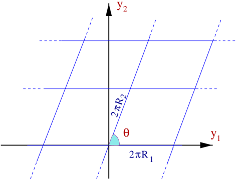
Figure 1: A two dimensional toroidal compactification constructed by identifying the opposite sites, with angle $\theta$ between the two cycles $\gamma_{1,2}$. The points $(y1,y2)$ and $(y_{1}+2\pi R_{1},y_{2})$ are identified; the same applies to $(y_{1},y_{2})$ and $(y_{1}+2\pi R_{2}\cos\theta,y_{2}+2\pi R_{2}\sin\theta)$. $\gamma_{1,2}$ are defined along $R_{1}$ and $R_{2}$ directions respectively and $A_{y_{1,2}}$ along the orthogonal dimensions $y_{1,2}$.

As in the previous section, a $y$-dependent transformation $V$ is introduced to “gauge away” the fields $A_{y_{1}}$, $A_{y_{2}}$. One finds that the new (transformed) fields must satisfy

$$A^{\prime}_{y_{1,2}}(x;y_{1},y_{2}) = 0\qquad\textrm{if}\qquad V(y_{1},y_{2})=e^{-iy_{1}A_{y_{1}}-iy_{2}A_{y_{2}}\quad}$$

$$A^{\prime}_{\mu}(x,y_{1},y_{2}) = VA_{\mu}(x,y_{1},y_{2})\,V^{-1}=A_{\mu}^{I}(x,y_{1},y_{2})T_{I}+A_{\mu}^{\alpha}(x,y_{1},y_{2})\,E_{\alpha}\,e^{-i(y_{1}A_{y_{1}}^{I}+y_{2}A_{y_{2}}^{I})\alpha^{I}}$$

$$\Phi^{\prime}(x;y_{1},y_{2}) = V\,\Phi(x;y_{1},y_{2})$$ (11)

with a summation over $I$ and $\alpha$ understood. With $T_{I}$, $E_{\alpha}$ linear independent one finds that the components $A_{\mu}^{I}$ are invariant under V, $A_{\mu}^{{}^{\prime}I}(x,y_{1},y_{2})=A_{\mu}^{I}(x,y_{1},y_{2})$ while $A_{\mu}^{\alpha}(x,y_{1},y_{2})$ may not necessarily be so. The initial periodicity conditions (2.3) are changed into

$$A_{\mu}^{{}^{\prime}\alpha}(x;y_{1}+2\pi R_{1},y_{2}) = e^{{-i2\pi R_{1}A_{y_{1}}^{I}\,\alpha_{I}}}\,\,A_{\mu}^{{}^{\prime}\alpha}(x;y_{1},y_{2})$$

$$A_{\mu}^{{}^{\prime}\alpha}(x;y_{1}+2\pi R_{2}\cos\theta,y_{2}+2\pi R_{2}\sin\theta) = e^{{-i2\pi R_{2}(A_{y_{1}}^{I}\cos\theta+A_{y_{2}}^{I}\sin\theta)\,\alpha_{I}}}\,\,A_{\mu}^{{}^{\prime}\alpha}(x;y_{1},y_{2})$$

$$\Phi_{\lambda}^{\prime}(x;y_{1}+2\pi R_{2}\cos\theta,y_{2}+2\pi R_{2}\sin\theta) = e^{{-i2\pi R_{2}(A_{y_{1}}^{I}\cos\theta+A_{y_{2}}^{I}\sin\theta)\,\lambda_{I}}}\,\,\Phi^{\prime}_{\lambda}(x;y_{1},y_{2})$$

$$\Phi^{\prime}_{\lambda}(x;y_{1}+2\pi R_{1},y_{2}) = e^{{-i2\pi R_{1}A_{y_{1}}^{I}}\,\lambda_{I}}\,\,\Phi^{\prime}_{\lambda}(x;y_{1},y_{2})$$ (12)

where $\Phi_{\lambda}$ denotes the component $\lambda$ of the multiplet $\Phi$ and where we used that $T_{I}\,\Phi_{\lambda}\,=\,\lambda_{I}\,\Phi_{\lambda}\,.$ A solution to these equations has the structure

$$\!\!\!\!\Psi^{\prime}_{\sigma}(x;y_{1},y_{2})\! \sim e^{-i(y_{1}A_{y_{1}}^{I}+iy_{2}A_{y_{2}}^{I})\,\sigma_{I}}\sum_{n_{1,2}\in{\bf Z}}\psi_{n_{1},n_{2},\sigma}(x)\,u_{n_{1},n_{2}}(y_{1},y_{2}),\quad\textrm{with}$$

$$\!\!\!\!u_{n_{1},n_{2}}(y_{1},y_{2})\!\! = \!\!\exp\bigg{[}i\frac{n_{1}}{R_{1}}\left(y_{1}-\frac{y_{2}}{\tan\theta}\right)\!+i\frac{n_{2}}{R_{2}}\frac{y_{2}}{\sin\theta}\bigg{]},\quad\Psi^{\prime}_{\alpha}\equiv\!A_{\mu}^{{}^{\prime}\alpha}\,\,and\,\,\Psi^{\prime}_{\lambda}\equiv\!\Phi^{\prime}_{\lambda};\,\,\sigma=\alpha,\,\lambda$$ (13)

where the field $\Psi^{\prime}$ is a notation for either $A_{\mu}^{{}^{\prime}\alpha}$ or $\Phi^{\prime}_{\lambda}$ while $\sigma_{I}$ denotes the roots $\alpha_{I}$ or the weights $\lambda_{I}$, respectively. $u_{n_{1},n_{2}}(y_{1},y_{2})$ is an eigenfunction of the Laplacian $\partial_{y_{1}}^{2}+\partial_{y_{2}}^{2}$ in the absence of the background gauge field because this was already “gauged away” in (2.3) (to derive $u_{n_{1},n_{2}}$ see for example [26]). If $\theta\!=\!\pi/2$, $u_{n_{1},n_{2}}(y_{1},y_{2})$ is a product of one-dimensional eigenfunctions for each $y_{i}$.

Using the Klein-Gordon equation in 6D for massless fields and the above mode expansion, one finds the mass of the Kaluza-Klein modes of 4D fields in the adjoint and fundamental representations

$$M^{2}_{n_{1},n_{2}}(\sigma) = \left[\frac{n_{1}}{R_{1}}-A_{y_{1}}^{I}\sigma_{I}\right]^{2}+\left[\frac{n_{2}}{R_{2}\sin\theta}-\frac{n_{1}}{R_{1}\tan\theta}-A_{y_{2}}^{I}\sigma_{I}\right]^{2}$$ (14)

$$\equiv \frac{1}{\sin\theta^{2}}\bigg{|}\,\frac{1}{R_{2}}(n_{2}+\rho_{2,\sigma})-\frac{e^{i\theta}}{R_{1}}(n_{1}+\rho_{1,\sigma})\bigg{|}^{2},\quad\sigma=\alpha\,\,\,or\,\,\,\sigma=\lambda$$

It turns out that $\rho_{i,\sigma}$, $i=1,2$ ($\sigma=\alpha,\lambda$) introduced in the last step in eq.(14) have values equal to those found in eq.(9) using the definition of eq.(2.1). Here $\sigma\!=\!\alpha$ ($\sigma\!=\!\lambda$) for the adjoint (fundamental) representation. (we will also use the notation $v_{\sigma}\equiv\sigma_{I}\!<\!A_{y_{1}}^{I}\!>$, $w_{\sigma}\equiv\sigma_{I}\!<\!A_{y_{1}}^{I}\!>$, (sum over $I$)).

If either $\rho_{1,\alpha}$, $\rho_{2,\alpha}$ are non-zero for a fixed $\alpha$, there is no massless “zero mode” $(n_{1},n_{2})=(0,0)$ boson in the associated Kaluza-Klein tower. The initial symmetry ${\cal G}$ is broken to a sub-group ${\cal G}^{*}$ generated by $T^{I}$ and those $E_{\alpha}$ for which $A_{\mu}^{{}^{\prime}\alpha}$ has a massless 4D zero-mode. This is controlled by the choice of $A_{y_{i}}^{I}$ vev’s in the root space of initial ${\cal G}$. The scale where ${\cal G}$ is broken to ${\cal G}^{*}$ depends on the the potential developed by $A_{y}$ fields and is thus model dependent (see [27] for an example). Further, in specific cases $\rho_{1,\sigma}$ and $\rho_{2,\sigma}$ may be simultaneously integers for a fixed $\sigma=\alpha$ or $\lambda$ and according to (14) (if $\sigma=\alpha$) there exists a massless Kaluza-Klein boson of non-zero level $(n_{1},n_{2})\not\!=\!(0,0)$. Consequently a gauge symmetry enhancement (beyond ${\cal G}^{*}$) takes place, enabled by additional corresponding $E_{\alpha}$. These results agree with the previous findings in Section 2.1.

One may regard the overall effect of symmetry breaking as a shift of the Kaluza-Klein levels $n_{i}$ to “effective” levels $n_{i,eff}\!=\!n_{i}+\rho_{i,\alpha}$ of non-integer values. The shift is due to the geometry of compactification, eq.(2.3) in the presence of constant background fields whose effect was replaced by “twisted” boundary conditions, eq.(2.3). Eq.(14) will be used in Section 3.2 to compute the radiative corrections to the 4D gauge coupling(s) of the group ${\cal G}^{*}$.

3 Wilson line corrections to 4D gauge couplings.

For realistic models ${\cal G}^{*}$ must include the Standard Model group (we will use $i=1,2,3$ to label its component groups); this can happen if ${\cal G}$ is SU(5). In general the group ${\cal G}$ may be larger and ${\cal G}^{*}$ contains additional group factors (not discussed). The coupling $g_{i}$ of a group factor $i$ of ${\cal G}^{*}$ is

$$\frac{4\pi}{g_{i}^{2}}\bigg{|}_{one-loop}=\frac{4\pi}{g_{i}^{2}}\bigg{|}_{tree-level}+\Omega_{i}^{T},\qquad\Omega_{i}^{T}\equiv\frac{1}{4\pi}\sum_{\psi}\tilde{\beta}_{i}(\psi)\int_{0}^{\infty}\frac{dt}{t}\,e^{-\pi\,tM^{2}_{\psi}/\mu^{2}}\bigg{|}_{reg.}$$ (15)

$\Omega_{i}^{T}$ sums all one-loop corrections to the coupling $g_{i}$, induced by the states $\psi$ of mass $M_{\psi}$. $\Omega_{i}^{T}$ is given by the Coleman-Weinberg formal equation in the rhs of eq.(15) (for a discussion see [7]). In (15) $\mu^{2}$ is a finite, non-zero mass parameter introduced to enforce a dimensionless equation; the subscript “reg” expresses that a regularisation of the integral is required.

$\Omega_{i}^{T}$ receives corrections from the 4D massless and massive fields charged under the group factor $i$ of ${\cal G}^{*}$. For our purpose we need not specify the 4D massless or Kaluza-Klein zero level spectrum, which depends on further details of the model considered. We restrict ourselves to computing the structure of the corrections to $\Omega_{i}^{T}$ from the 4D massive sector and we sum over all Kaluza-Klein towers of states charged under the group $i$ of ${\cal G}^{*}$. These are: (1). 4D Kaluza-Klein towers of states whose levels are not shifted (i.e. $\rho_{k,\sigma}=0$, $k=1,2$) and have massless zero-modes. An example is (if $\sigma=\alpha$) that of Kaluza-Klein states associated with the “unbroken” generators $E_{\alpha}$ (of the group $i$ of ${\cal G}^{*}$) and: (2). 4D Kaluza-Klein towers of states of levels shifted by the amount $\rho_{k,\sigma}$, $k=1,2$. An example is (if $\sigma=\alpha$) that of Kaluza-Klein states associated with the “broken” generators $E_{\alpha}$ (like $X,Y$ gauge bosons and their Kaluza-Klein tower for the SU(5) breaking to the SM group).

For the beta functions $\beta_{i}$ one has (after suppressing the subscript $i$) that $\tilde{\beta}(\sigma)=k_{r}(\sigma_{I}\sigma^{I})/{\textrm{rk}{\cal G}^{*}}$ for $\sigma$ belonging to representation $r$; $k_{r}=\{-11/3,2/3,1/3\}$ for adjoint representations, Weyl fermion and scalar respectively. The Dynkin index $T(r)=(\sum_{\sigma}\sigma_{I}\sigma^{I})_{r}/(rk{\cal G}^{*})$ where the sum is over all weights/roots $\sigma$ belonging to representation $r$, each occurring a number of times equal to its multiplicity [25]. With the definition $b_{i}(r)\equiv\sum_{\sigma}\tilde{\beta}_{i}(\sigma)$ for the weights $\sigma$ belonging to $r$ one has $b_{i}\!=\!-11/3\,T_{i}(A)~{}+~{}2/3\,T_{i}(R)~{}+~{}1/3\,T_{i}(S)$, to account for the adjoint, Weyl fermion in representation $R$ and scalar in representation $S$. Massive N=1 Kaluza-Klein states can be organised as N=2 hypermultiplets with $b_{i}=2T_{i}(R)$ and N=2 vector supermultiplets with $b_{i}=-2T_{i}(A)$.

3.1 One extra-dimension and Wilson line corrections.

For the case of one additional compact dimension $\Omega_{i}^{T}$ can be written as

$$\Omega_{i}^{T}=\sum_{r}\sum_{\sigma=\lambda,\alpha}\Omega_{i}(\sigma),\qquad\quad\Omega_{i}(\sigma)\equiv\frac{1}{4\pi}\sum_{m\in{\bf Z}}\tilde{\beta}_{i}(\sigma)\int_{\xi}^{\infty}\frac{dt}{t}\,e^{-\pi\,t\,M^{2}_{m}(\sigma)/\mu^{2}}e^{-\pi\chi t}$$ (16)

$\Omega_{i}(\sigma)$ is the contribution of a tower of Kaluza-Klein modes associated with a state $\sigma$ “shifted” by $\rho(\sigma)$ real, with $\sigma=\lambda,\alpha$ the weight/root belonging to the representation r. The sum over $m$ runs over all integers, representing Kaluza-Klein levels of mass $M_{m}(\sigma)$ given by eq.(2.2)

$$M_{m}(\sigma)=(m+\rho_{\sigma})^{2}/R^{2},\qquad\rho_{\sigma}=-R<\!A_{y}^{I}\!>\sigma_{I}\equiv-R\,v_{\sigma};\quad\sigma=\alpha,\lambda.$$ (17)

with $\sigma=\alpha$, $(\lambda)$ for the adjoint (fundamental) representation. In eq.(16) a regularisation of the integral was performed. Since $\Omega_{i}^{T}$ is UV divergent ($t\rightarrow\!0$) an UV regulator $\xi\rightarrow 0$ was introduced as the lower limit of the integral. For the special case when there are massless states in the Kaluza-Klein tower, the integral is also IR divergent $(t\rightarrow\!\infty)$ and an IR regulator $\chi\rightarrow 0$ is introduced. If no massless states exist in the Kaluza-Klein tower, one formally sets $\chi=0$. For other regularisations and their relationship with that employed here see Appendix A-4 of this work and Appendix B, C of [11]. From eq.(16) the relation between the UV/IR regulators and their associated mass scales can be inferred to be of type $\Lambda^{2}\propto\mu^{2}/\xi$ for the UV scale and $Q^{2}\propto\chi\mu^{2}$ for the IR scale.

As usually done when computing the one-loop corrections in 4D compactified models [7], [9] we isolate in eq.(16) the contribution of the “zero” modes (whose existence is model dependent, they may be projected out by the initial orbifolding) from that of the non-zero level modes, which is general and is computed in string case. To keep track of this separation we re-label by $\beta_{i}(\sigma)$    (${\overline{\beta}}_{i}(\sigma)$) the one loop beta function of “zero” (non-zero) modes, respectively. In the following the dependence of $\rho$, $\overline{\beta}$, $\beta$ and $M_{m}$ on $\sigma=\alpha,\lambda$ is not written explicitly. From (16) we have

$$\Omega_{i}=\frac{\beta_{i}}{4\pi}{\cal J}^{0}+\frac{\overline{\beta}_{i}}{4\pi}{\cal J}$$ (18)

with the notation

$$\!\!\!\!\!\!\!\!\ {\cal J}^{0} \equiv \int_{\xi}^{\infty}\frac{dt}{t}\,e^{-\pi\,t\,M_{0}^{2}/\mu^{2}}e^{-\pi\chi\,t}=\Gamma[0,\pi\nu\xi(\rho^{2}+\chi/\nu)],\qquad\qquad\nu\equiv\frac{1}{(R\mu)^{2}}$$

$$\!\!\!\!\!{\cal J} \equiv \sum_{m\in{\bf Z}}^{\prime}\int_{\xi}^{\infty}\frac{dt}{t}\,e^{-\pi\,t\,M_{m}^{2}/\mu^{2}}e^{-\pi\chi\,t}$$ (19)

$$= \frac{2e^{-\pi\xi\chi}}{\sqrt{\nu\xi}}-\Gamma[0,\pi\nu\xi(\rho^{2}+\chi/\nu)]+2\pi({\chi}/{\nu})^{\frac{1}{2}}\textrm{Erf}[\sqrt{\pi\xi\chi}]-\ln\Big{|}2\sin\pi[\rho+i({\chi}/{\nu})^{\frac{1}{2}}]\Big{|}^{2}$$

with the functions $\Gamma[0,x]$ and Erf[$x$] defined in the Appendix eq.(A.1). A “prime” on the sum over “m” indicates that the sum is over all integers $m$ with $m\not=0$. To evaluate ${\cal J}$ the results of Appendix A.1, eq.(A-1) were used. Eq.(19) is valid if

$$\nu\,\xi\ll 1,\qquad\textrm{or}\qquad\frac{1}{R^{2}}\ll\frac{\mu^{2}}{\xi}$$ (20)

Eqs.(16) to (20) give the most general result for the radiative correction to gauge couplings. In the limit of “removing” the regulators dependence ($\xi\rightarrow 0$) the $\Gamma$ functions contributions in ${\cal J}^{0}$, ${\cal J}$ can be approximated by logarithms while the Erf function contribution vanishes. The presence of the regulator $\chi$ ensures that the result (19) applies whether or not there are massless states in the Kaluza-Klein tower.

The mass parameter $\mu$ combines with the (dimensionless) regulators $\xi$ and $\chi$ to introduce the following associated mass scales

$$Q^{2}\equiv\pi e^{\gamma}\chi\,\mu^{2}\bigg{|}_{\chi\rightarrow 0}\,\qquad\Lambda^{2}\equiv\frac{\mu^{2}}{\xi}\bigg{|}_{\xi\rightarrow 0}\$$ (21)

$Q$ is therefore the low(est) energy scale, and $\Lambda$ is the high(est) energy (UV) scale of the theory. With this notation the one-loop correction is

$$\!\!\!\!\!\!\!\!\rho=0: \!\!\Omega_{i}=\frac{\beta_{i}}{4\pi}\ln\frac{\Lambda^{2}}{Q^{2}}-\frac{\overline{\beta}_{i}}{4\pi}\ln\bigg{[}4\pi e^{-\gamma}(\Lambda R)^{2}\,e^{-2\Lambda R}\bigg{]},$$ (22)

$$\!\!\!\!\!\!\!\!\rho\!\in\!{\bf Z}^{*}: \!\!\Omega_{i}=\frac{\beta_{i}}{4\pi}\ln\frac{\Lambda^{2}}{Q^{2}}-\frac{\overline{\beta}_{i}}{4\pi}\ln\bigg{[}4\pi e^{-\gamma}(\Lambda R)^{2}\,e^{-2\Lambda R}\bigg{]}+\frac{{\overline{\beta_{i}}}-\beta_{i}}{4\pi}\ln\bigg{[}1+\frac{\pi e^{\gamma}(\rho/R)^{2}}{Q^{2}}\bigg{]}$$ (23)

$$\!\!\!\!\!\!\!\!\!\!\!\!\!\!\!\!\rho\not\in\!{\bf Z}: \!\!\Omega_{i}=\frac{\beta_{i}}{4\pi}\ln\frac{\Lambda^{2}}{Q^{2}}-\!\frac{\overline{\beta}_{i}}{4\pi}\ln\bigg{[}4\pi e^{-\gamma}(\Lambda R)^{2}\,e^{-2\Lambda R}\bigg{]}-\!\frac{\overline{\beta}_{i}}{4\pi}\!\ln\bigg{[}\frac{\sin(\pi\rho)}{\pi\rho}\bigg{]}^{2}\!\!\!\!-\frac{\beta_{i}}{4\pi}\ln\bigg{[}\frac{\!\pi e^{\gamma}(\rho/R)^{2}}{\!\!Q^{2}}\bigg{]}$$ (24)

where according to eq.(17), $\rho/R$ is a vacuum expectation value in a direction in the weight/root space. These equations are valid if the following conditions are respected:

$$\rho=0: Q^{2}\ll\frac{1}{R^{2}}\ll\Lambda^{2}$$ (25)

$$\rho\in{\bf Z}^{*}: Q^{2}\ll\frac{1}{R^{2}}\ll\Lambda^{2}\quad\textrm{and}\quad\frac{\rho^{2}}{R^{2}}\ll\Lambda^{2}$$ (26)

$$\rho\not\in{\bf Z}: \frac{1}{R^{2}}\ll\Lambda^{2}\quad\textrm{and}\quad\frac{\rho^{2}}{R^{2}}\ll\Lambda^{2}$$ (27)

Eqs.(22) to (27) provide the threshold correction to the gauge couplings at one-loop level due to a tower of Kaluza-Klein states in the presence/absence of a constant background gauge field.

The first logarithmic term in eqs.(22), (23), (24) stands for the contribution of the “zero” modes from the high scale $\Lambda$ to some low energy scale $Q$. The second term in these equations proportional to $\overline{\beta}_{i}$ contains the linear contribution (in $\Lambda$) to the gauge couplings and is due to the Kaluza-Klein states of the extra-dimension, in the absence of Wilson lines [11]. Eq.(22) gives the correction for the case of vanishing Wilson line vev’s ($\rho=0$).

For the case $\rho\in{\bf Z}^{*}$ the last term in eq.(23) gives an additional contribution due to the Wilson line vev’s. Note that this correction is proportional to beta functions differences of zero and non-zero levels which may actually vanish in specific cases. The correction also depends on the low energy scale $Q$ brought in by the need for an IR regulator when $\rho\in{\bf Z}^{*}$. Consequently, the low energy physics represented by $Q$ is related to Wilson line effects, even though the latter may take place at a very high energy scale or may have a large vev ($\rho$) compared to $Q$. Formally, if one sets $\rho=0$ the case of eq.(22) is recovered. Finally, the constraint (26), $\rho/R\ll\Lambda$ may be “relaxed” into $\rho/R\leq\Lambda$ or $\rho/R\approx\Lambda$ if one uses eq.(18), (19), (20) instead of (23), (26).

The result for the case with $\rho\not\in{\bf Z}$ does not depend on $Q$ (the dependence displayed in (24) cancels out). For $\Omega_{i}(\rho\!\not\in\!{\bf Z})$ the limit of reaching an integer or vanishing $\rho$ is not finite, see the last two terms in (24). Indeed, the one loop correction has an infrared divergence at integer and vanishing values of $\rho$, which are “moduli” points where new massless states appear. If these correspond to vector superfields ($\sigma=\alpha$) the symmetry ${\cal G}^{*}$ is enlarged. Therefore these “moduli” points cannot be smoothly reached perturbatively by taking the limit of integer $\rho$.

We are now able to write the most general threshold correction to the gauge couplings by combining the contributions $\Omega_{i}$ for all possible values for $\rho_{\sigma}$. Making the dependence on $\sigma$ manifest, one has from (16) and (22) to (24)

$$\Omega_{i}^{T}=\sum_{r}\sum_{\sigma=\alpha,\lambda}\Big{[}\Omega_{i}(\rho_{\sigma}=0)+\Omega_{i}(\rho_{\sigma}\in{\bf Z}^{*})+\Omega_{i}(\rho_{\sigma}\not\in{\bf Z})\Big{]}$$ (28)

with the remark that if the condition for the argument of any term $\Omega_{i}$ is not respected, that term in the sum should be set to zero. Conditions (25) to (27) should be considered accordingly.

3.2 Two extra-dimensions and Wilson line corrections.

The effects on the gauge couplings of the 4D Kaluza-Klein states in the presence of a background (gauge) field are similar to the one-dimensional case. Eq.(15) becomes

$$\Omega_{i}^{T}\equiv\sum_{r}\sum_{\sigma=\alpha,\lambda}\Omega_{i}(\sigma),\qquad\Omega_{i}(\sigma)\equiv\frac{1}{4\pi}\sum_{m_{1,2}\in{\bf Z}}\tilde{\beta}_{i}(\sigma)\int_{\xi}^{\infty}\frac{dt}{t}\,e^{-\pi\,tM^{2}_{m_{1},m_{2}}(\sigma)/\mu^{2}}\,e^{-\pi\chi\,t}.$$ (29)

with a summation over all weights/roots belonging to representation $r$. As in the one dimensional case an UV regulator $\xi$ ($\xi\!\rightarrow\!0$) is introduced since the integral is divergent at $t\!\rightarrow\!0$ and the associated UV scale is then proportional to $\mu^{2}/\xi$. For special values of Kaluza-Klein levels $(m_{1},m_{2})$ and Wilson lines vev’s (see eq.(14)), $M_{m_{1},m_{2}}$ may vanish, and the integral becomes infrared divergent ($t\!\rightarrow\!\infty$). An IR regulator $\chi$ is introduced $\chi\!\rightarrow\!0$ for these particular cases, with associated infrared scale $Q^{2}\propto\mu^{2}\chi$. The regulator plays the role of a 6D mass term in the Klein-Gordon equation which shifts the value of $M_{m_{1},m_{2}}$ in eq.(14). The cases with $M_{m_{1},m_{2}}\!=\!0$ for Kaluza-Klein bosonic states of non-zero level are important since they signal an enlargement of the gauge symmetry ${\cal G}^{*}$. The mass of the Kaluza-Klein states given in (14) can be written as

$$M^{2}_{m_{1},m_{2}}(\sigma) = \frac{\mu^{2}}{T_{2}U_{2}}\,|m_{2}+\rho_{2,\sigma}-U(m_{1}+\rho_{1,\sigma})|^{2},\quad\sigma=\alpha,\lambda.$$ (30)

with the notation

$$U\equiv U_{1}+iU_{2}=R_{2}/R_{1}\,e^{i\theta},\,\,\,\,(U_{2}>0);\,\qquad{T}(\mu)\equiv i\,T_{2}(\mu)=i\mu^{2}R_{1}R_{2}\sin\theta\,.$$ (31)

The structure of the mass formula (30) is very general and also applies to string compactifications. At the string level $U$ and $T$ have correspondents in the so-called moduli fields related to the complex structure and (imaginary part of) the Kähler structure of the two-torus respectively. The notation in eq.(31) is introduced to facilitate a comparison with the string results where this notation is standard. $\rho_{1,2}$ are related to the Wilson line vev’s, see eq.(9), (14). The mass (30) equals that encountered in (heterotic) string compactification for zero winding modes. This is expected, since an effective field theory approach corresponds to the case of an infinite string scale when winding modes are infinitely heavy and their effects are suppressed.

To compute $\Omega_{i}^{T}$ of (29) we isolate the contribution of $(0,0)$ mode from that of the rest of the Kaluza-Klein modes (this is allowed after the regularisation of the integral in (29)). This separation is needed for two reasons. First, the exact final spectrum of zero level or massless modes depends on further details of the models considered; in particular some $(0,0)$ modes may not “survive” the initial orbifold projections. Second, string calculations of $\Omega_{i}$ [9], [20] that we want to compare with only compute the effects of the non-zero levels. To keep track of this mode separation we re-label $\tilde{\beta}_{i}$ by $\overline{\beta}_{i}$ ($\beta_{i}$) for the Kaluza-Klein levels $(m_{1},m_{2})\not=(0,0)$, ($(m_{1},m_{2})=(0,0)$) respectively.

The analysis below considers separately Case 1 of vanishing Wilson lines vev’s $\rho_{k,\sigma}=0$, $k=1,2$ ($\sigma$ fixed) as a reference for when we evaluate Case 2 of non-vanishing Wilson vev’s. Case 2 (B) when the Wilson line breaks the gauge symmetry is the most interesting for phenomenology.

3.2.1 Case 1. Wilson line background absent.

In this case there are vanishing vev’s of the Wilson lines $\rho_{k,\sigma}=0$, $k=1,2$ for a particular set of $\sigma=\alpha,\lambda$, with corresponding $E_{\alpha}$ as unbroken generators. If this is true for all $\alpha$ there is no breaking of the initial symmetry ${\cal G}$. For simplicity we assume this is indeed the case, otherwise the discussion refers to the unbroken part ${\cal G}^{*}$ of ${\cal G}$ only and the effect of Kaluza-Klein towers “not shifted” by $\rho_{k,\alpha}$. Therefore the problem is that of one-loop corrections to the gauge couplings due to the N=2 sector (of a 4D N=1 orbifold) compactified on a two-torus (no Wilson lines vev’s) and well-known in the heterotic string [9]. At the effective field theory level this calculation was performed in [11], [12], reviewed here for later reference. In eq.(29) the mass of the Kaluza-Klein states does not depend on $\sigma$ and the sum of $\tilde{\beta}_{i}(\sigma)$ over $\alpha,\lambda$, $r$ (for the group ${\cal G}$!) may be performed before the integral itself. We denote this overall sum by $b_{i}$, $\overline{b}_{i}$ for $(0,0)$ and for $(m_{1},m_{2})\not=(0,0)$ modes respectively. The total correction $\Omega_{i}^{T}$ has then the structure

$$\Omega_{i}^{T}=\frac{b_{i}}{4\pi}{\cal J}_{0}^{(1)}+\frac{\overline{b}_{i}}{4\pi}{\cal J}^{(1)}$$ (32)

with

$${\cal J}_{0}^{(1)} \equiv \int_{\xi}^{\infty}\frac{dt}{t}\,e^{-\pi tM_{0,0}^{2}/\mu^{2}}\,e^{-\pi\chi t}\,=\int_{\xi}^{\infty}\frac{dt}{t}e^{-\pi\chi t}=\Gamma[0,\pi\xi\chi]$$

$${\cal J}^{(1)} \equiv \sum_{m_{1,2}}^{\prime}\int_{\xi}^{\infty}\frac{dt}{t}e^{-\pi\,t\,M_{m_{1},m_{2}}^{2}/\mu^{2}}e^{-\pi\chi t}=\sum_{m_{1,2}}^{\prime}\int_{\xi}^{\infty}\frac{dt}{t}e^{-\frac{\pi\,t}{T_{2}U_{2}}\,|m_{2}-Um_{1}|^{2}-\pi\chi t}$$ (33)

$$= -\ln\left[4\pi e^{-\gamma}\,e^{-\frac{T_{2}}{\xi}}\,\frac{T_{2}}{\xi}U_{2}\left|\eta(U)\right|^{4}\right]+\pi\chi T_{2}\ln\bigg{[}4\pi e^{-\gamma}U_{2}\frac{\xi}{T_{2}}\bigg{]}$$

and with

$$\chi\ll\min\left\{{U_{2}}/{T_{2}},{1}/{(T_{2}U_{2})}\right\};\qquad\max\left\{{U_{2}}/{T_{2}},{1}/({T_{2}U_{2}})\right\}\ll{1}/{\xi}$$ (34)

A “prime” on a double sum stands for a sum over all integers $(m_{1},m_{2})$ except the mode $(0,0)$ considered by ${\cal J}_{0}^{(1)}$. An infrared regulator was introduced in $\Omega_{i}^{T}$ before its splitting into ${\cal J}_{0}^{(1)},{\cal J}^{(1)}$, because $M_{0,0}=0$ according to (30). The correction ${\cal J}^{(1)}$ was evaluated in detail in ref.[12]. Condition (34) ensures that higher order corrections in the regulators $\chi$ and $\xi$ vanish in the limit of removing them, $\chi,\,\xi\rightarrow 0$. From (33) one finds the overall correction to the gauge couplings due to the towers of Kaluza-Klein states associated with two dimensions (and vanishing Wilson line vev’s)

$$\Omega_{i}^{T}=\frac{b_{i}}{4\pi}\ln\frac{\Lambda^{2}}{Q^{2}}-\frac{{\overline{b}}_{i}}{4\pi}\ln\Big{[}4\pi e^{-\gamma}\,e^{-{T_{2}^{*}}}\,{T_{2}^{*}}\,U_{2}\,|\eta(U)|^{4}\Big{]}+\frac{{\overline{b}}_{i}}{4\pi}Q^{2}R_{1}R_{2}\sin\theta\,e^{-\gamma}\ln\bigg{[}4\pi e^{-\gamma}\frac{U_{2}}{T_{2}^{*}}\bigg{]}$$ (35)

We introduced the notation

$$T_{2}^{*}\equiv\left.\,\frac{T_{2}}{\xi}\,\right|_{\xi\rightarrow 0}=\Lambda^{2}R_{1}R_{2}\sin\theta,\qquad\quad\textrm{and}\qquad\left.\Lambda^{2}\equiv\frac{\mu^{2}}{\xi}\right|_{\xi\rightarrow 0},\qquad Q^{2}\equiv\pi e^{\gamma}\,\mu^{2}\chi\,\bigg{|}_{\chi\rightarrow 0}$$ (36)

which will be used in the remaining sections. Eq.(34) becomes

$$Q\ll\min\left\{\frac{1}{R_{1}},\frac{1}{R_{2}\sin\theta}\right\};\qquad\max\left\{\frac{1}{R_{1}},\frac{1}{R_{2}\sin\theta}\right\}\ll\Lambda$$ (37)

which implies $\Lambda^{2}R_{1}R_{2}\sin\theta\gg 1$ i.e. a large area of compactification (in UV scale units). Note that $(R_{2}\sin\theta)$ plays the role of an “effective” radius of the extra dimension. Eq.(36) clarifies the link between the UV/IR regulators and the mass scales $\Lambda$ and $Q$ which emerge as corresponding UV and IR cut-off scales respectively.

The first term in $\Omega_{i}^{T}$ is the usual one-loop logarithmic correction which accounts for the effects of $(0,0)$ modes, from the high scale $\Lambda$ to the low energy scale $Q$. The second term accounts for the effects of the massive Kaluza Klein states associated with the two extra dimensions and shows the usual power-like dependence [6] on the UV scale since $\Omega_{i}^{T}\sim T_{2}^{*}\sim\Lambda^{2}$. Its structure can be compared with that of the corresponding (heterotic) string result in the limit of an infinite string scale or $\alpha^{\prime}\rightarrow 0$, when the additional effects of the winding states of the string are minimised. The string result in this limit agrees with that of field theory. For a detailed discussion on the second term in $\Omega_{i}^{T}$ and its link with the heterotic string see [11].

There remains the last term in $\Omega_{i}^{T}$ i.e. $Q^{2}R_{1}R_{2}\sin\theta\ln U_{2}/T_{2}^{*}\sim\chi\ln\xi$ whose origin was analysed in detail in [12]. Here we review briefly its significance. This correction arises from the UV divergent contribution ${\cal J}^{(1)}$ of the massive momentum states in the presence of the infrared regulator $\chi$. The latter was required by the (IR divergent) contribution of the massless mode $M_{0,0}$. Therefore the term $\chi\ln\xi$ establishes an (infrared) link between the massive and massless sectors. The term $\chi\ln\xi$ or the last term in $\Omega_{i}^{T}$ that it induces must be kept in the final correction to the gauge couplings because the limits of removing the regulators $\chi\rightarrow 0$ and $\xi\rightarrow 0$ do not commute.

The presence of the last term in $\Omega_{i}^{T}$ shows that even though Kaluza-Klein states may have a very large mass, of the order of the compactification scales, their overall contribution is still proportional to a much lower scale $Q$, where they may actually be decoupled. The contribution of this term may be large since $U_{2}\ll T_{2}^{*}$ (equivalently $1/R_{1}\ll\Lambda$). However the coefficient in front may be small $Q^{2}R_{1}R_{2}\sin\theta\ll 1$ for our result to be accurate, see conditions in eq.(37). We conclude that the overall effect of the infinite tower of Kaluza-Klein states on the gauge couplings cannot be split into massless and massive modes only, and a combined effect of these mass sectors through infrared effects is present.

The last term in $\Omega_{i}^{T}$ has no equivalent at the string level [12]. To understand why this is so, note that at the string level, the UV regulator $\xi\propto 1/\Lambda^{2}$ has a “correspondent” in $\alpha^{\prime}\propto 1/M_{s}^{2}$ with the limit $\xi\rightarrow 0$ to correspond to an infinite string scale or $\alpha^{\prime}\!\rightarrow\!0$. String calculations of $\Omega_{i}^{T}$ require an infrared regularisation, so $\chi$ also has a string infrared regulator correspondent that we denote $\epsilon$, with $\epsilon\rightarrow 0$. Therefore, a string equivalent of the last term in $\Omega_{i}^{T}$ would be $\epsilon\ln\alpha^{\prime}$. Such term does appear in string calculations during the string infrared regularisation (see [12] and Appendix A of [28]). However in string calculations $\alpha^{\prime}\not=0$ and consequently $\epsilon\ln\alpha^{\prime}\rightarrow 0$ in the final, infrared regularised string result when $\epsilon\rightarrow 0$. The subsequent “field theory” limit $\alpha^{\prime}\rightarrow 0$ of this string result will then miss the last term in $\Omega_{i}^{T}$. The origin of this discrepancy is that in specific cases (such as two extra-dimensions) the infrared regularisation of the (world-sheet integral of the) string and its “field theory” limit $\alpha^{\prime}\rightarrow 0$ do not commute.

The conclusion is that the UV behaviour found using effective field theory methods for a 4D N=1 orbifold compactification with N=2 sub-sector (two-torus) is not necessarily that of its (infrared regularised) string embedding in the limit $\alpha^{\prime}\rightarrow 0$. This issue is closely related to the infinite number of states in the Kaluza-Klein tower that one sums over, which bring about a “non-decoupling” of the UV effects from the low energy ($Q$) sector. This concludes our review of the radiative corrections to the couplings for vanishing Wilson lines vev’s. For more details on this issue see [12].

3.2.2 Case 2. Wilson lines background present.

In this case there is a non-zero Wilson lines background $\rho_{i,\sigma}$, $i=1,2$, $\sigma=\alpha,\lambda$, that can in some cases ($\sigma=\alpha$) affect the symmetry ${\cal G}^{*}$. We distinguish two general possibilities for $\Omega_{i}(\sigma)$ of eq.(29)

(A). $\rho_{1,\sigma}\in{\bf Z}$, $\rho_{2,\sigma}\in{\bf Z}$ ($\sigma$ fixed), and

(B). $\rho_{1,\sigma}\not\in{\bf Z}$ and $\rho_{2,\sigma}$ real (or $\rho_{2,\sigma}\not\in{\bf Z}$ and $\rho_{1,\sigma}$ real)

Case 2 (A). Computing $\Omega_{i}$ for $\rho_{1,\sigma}\in{\bf Z}$, $\rho_{2,\sigma}\in{\bf Z}$.

In this case there exists a non-zero Wilson lines vev, with $\rho_{i,\sigma}$, $i=1,2$ simultaneously integers, for a fixed $\sigma=\alpha$ or $\lambda$. Therefore for a specific value of the Kaluza-Klein levels, $M_{m_{1},m_{2}}(\sigma)$ vanishes and if this corresponds to a bosonic state $\alpha$, an enlargement of the gauge symmetry ${\cal G}^{*}$ takes place. When $M_{m_{1},m_{2}}(\sigma)$ vanishes an infrared regulator $\chi$ is required for the corresponding tower of Kaluza-Klein states which contributes to $\Omega_{i}(\sigma)$. This is given by (below the $\sigma$ dependence will not be written explicitly)

$$\Omega_{i}=\frac{\beta_{i}}{4\pi}{\cal J}_{0}^{(2)}+\frac{\overline{\beta}_{i}}{4\pi}{\cal J}^{(2)}$$ (38)

where we isolated the contribution ${\cal J}_{0}^{(2)}$ of the $(0,0)$ mode with beta function $\beta_{i}$, from that of non-zero modes ${\cal J}^{(2)}$ with beta function ${\overline{\beta}_{i}}$ and

$${\cal J}_{0}^{(2)} \equiv \int_{\xi}^{\infty}\frac{dt}{t}e^{-\pi\,t\,M_{0,0}^{2}}\,e^{-\pi\chi t}=\int_{\xi}^{\infty}\frac{dt}{t}e^{-\frac{\pi t}{T_{2}U_{2}}\,|\rho_{2}-U\rho_{1}|^{2}-\pi\chi t}=\Gamma\Big{[}0,\pi\xi\Big{(}\!|\rho_{2}-U\rho_{1}|^{2}/(T_{2}U_{2})+\chi\Big{)}\!\Big{]}$$

$${\cal J}^{(2)} \equiv \sum_{m_{1,2}}^{\prime}\int_{\xi}^{\infty}\frac{dt}{t}e^{-\pi\,t\,M_{m_{1},m_{2}}^{2}/\mu^{2}}\,e^{-\pi\chi t}=\sum_{m_{1,2}}^{\prime}\int_{\xi}^{\infty}\frac{dt}{t}e^{-\frac{\pi\,t}{T_{2}U_{2}}\,|m_{2}+\rho_{2}-U(m_{1}+\rho_{1})|^{2}-\pi\chi t}$$ (39)

$$= {\cal J}^{(1)}+\Gamma\Big{[}0,\pi\xi\chi\Big{]}-\Gamma\Big{[}0,\pi\xi\Big{(}|\rho_{2}-U\rho_{1}|^{2}/(T_{2}U_{2})+\chi\Big{)}\!\Big{]}$$

with

$$\chi\ll\min\left\{{U_{2}}/{T_{2}},{1}/{(T_{2}U_{2})}\right\}\leq\max\left\{{U_{2}}/{T_{2}},{1}/({T_{2}U_{2}})\right\}\ll{1}/{\xi}$$ (40)

For a simple evaluation of ${\cal J}^{(2)}$ one adds and subtracts under its integral the exponential evaluated for $(m_{1},m_{2})=(0,0)$, then shifts the summation variables $m_{1,2}$ by the integers $\rho_{1,2}$ respectively and finally isolates from the sum the “new” $(0,0)$ mode. One then recovers an integral equal to ${\cal J}^{(1)}$ of eq.(33) plus two additional terms, giving the result (39).

Using the notation introduced in eq.(36) we obtain from (38) and (39) the result

$$\Omega_{i} = \frac{\beta_{i}}{4\pi}\ln\frac{\Lambda^{2}}{Q^{2}}-\frac{{\overline{\beta}}_{i}}{4\pi}\ln\Big{[}4\pi e^{-\gamma}\,e^{-{T_{2}^{*}}}\,{T_{2}^{*}}\,U_{2}\,|\eta(U)|^{4}\Big{]}+\frac{{\overline{\beta}}_{i}}{4\pi}Q^{2}R_{1}R_{2}\sin\theta\,e^{-\gamma}\ln\bigg{[}4\pi e^{-\gamma}\frac{U_{2}}{T_{2}^{*}}\bigg{]}$$ (41)

$$+ \frac{{\overline{\beta}_{i}}-\beta_{i}}{4\pi}\ln\bigg{[}1+\frac{\pi e^{\gamma}|\rho_{2}-U\rho_{1}|^{2}}{Q^{2}(R_{2}\sin\theta)^{2}}\bigg{]}$$

with

$$Q\ll\min\left\{\frac{1}{R_{1}},\frac{1}{R_{2}\sin\theta}\right\};\qquad\max\left\{\frac{1}{R_{1}},\frac{1}{R_{2}\sin\theta},\frac{|\rho_{2}-U\rho_{1}|}{R_{2}\sin\theta}\right\}\ll\Lambda$$ (42)

Except its last term, the result for $\Omega_{i}$ is similar to that for vanishing Wilson lines discussed in Case 1. The first, second and third terms in (41) account for the effects of the $(0,0)$ modes, massive Kaluza-Klein modes alone and the “mixed” contribution proportional to $Q^{2}$, respectively. However, there exists an additional term proportional to $({\overline{\beta}_{i}}-\beta_{i}$), not present in Case 1, and this is due to the effects of the Wilson lines alone. This term vanishes if one formally sets $\rho_{1}=\rho_{2}=0$ when Case 1 is recovered. Note the similarity of the last term in $\Omega_{i}$ to that of the last term in (23) of the one extra-dimension case. The Wilson line contribution can also be written as

$$\frac{{\overline{\beta}_{i}}-\beta_{i}}{4\pi}\ln\bigg{[}1+\frac{\pi e^{\gamma}(v_{\sigma}^{2}+w_{\sigma}^{2})}{Q^{2}}\bigg{]},\qquad v_{\sigma}\equiv\sigma_{I}\!<\!A_{y_{1}}^{I}\!>,\quad w_{\sigma}\equiv\sigma_{I}\!<\!A_{y_{2}}^{I}\!>,\quad\sigma=\alpha,\lambda.$$ (43)

where $v_{\sigma}$ and $w_{\sigma}$ denote a vev in a direction in the root ($\alpha$) or weight ($\lambda$) space. Note that $\beta_{i}$ and ${\overline{\beta}_{i}}$ depend on $\sigma$. This is relevant when the sum over $\sigma$ of eq.(29) is performed to compute total $\Omega_{i}^{T}$.

The correction due to Wilson lines vev’s shows how the couplings change when non-zero level Kaluza-Klein modes become massless. The correction due to the Wilson lines in eq.(41) depends on their vev’s and on the low scale $Q$, but the ultraviolet behaviour of the models is not changed. Indeed the $T_{2}^{*}\sim\Lambda^{2}$ dependence of $\Omega_{i}$ is identical to that of the case with vanishing Wilson lines vev’s addressed in the previous section. Regarding the $Q$ dependence of $\Omega_{i}$ we remark the following. The gauge couplings are changed at the low scale $Q$ as a result of (possibly) large Wilson lines vev’s $\rho_{i}$ and of their near-cancellations against large Kaluza-Klein levels $(m_{1},m_{2})$ corresponding to a large momentum in the compact directions $m_{1,2}/R_{1,2}$ and giving $M_{m_{1},m_{2}}\approx 0$.

Case 2 (B). Computing $\Omega_{i}$ for $\rho_{1,\sigma}\not\in{\bf Z}$, $\rho_{2,\sigma}$ real (or $\rho_{2,\sigma}\not\in{\bf Z}$, $\rho_{1,\sigma}$ real).

In the following we assume $\rho_{1,\sigma}\!\not\in\!{\bf Z}$ and $\rho_{2,\sigma}$ real. (Appendix B extends this analysis to $\rho_{2,\sigma}\not\in{\bf Z}$, $\rho_{1,\sigma}$ real). Phenomenologically this is the most interesting case we discuss. There are non-zero Wilson line vev’s and $M_{m_{1},m_{2}}(\sigma)\!\not=\!0$ for a fixed set of $\sigma=\lambda,\alpha$. The corresponding generators $E_{\alpha}$ are broken, the symmetry is (reduced to) ${\cal G}^{*}$ and Kaluza-Klein towers are “shifted” (by $\rho_{i,\sigma}$). Since there is no massless state for any integers $m_{1},m_{2}$, in eq.(29) there is no need for an IR regulator $\chi$ for the corresponding correction $\Omega_{i}(\sigma)$ of the Kaluza-Klein tower. In the following the $\sigma$ dependence is not shown explicitly. After Poisson re-summation (A-2) the integrand in (29) becomes

$$\sum_{m_{1},m_{2}}^{\prime}e^{-\pi tM_{m_{1},m_{2}}^{2}/\mu^{2}} = \sum_{m_{2}}^{\prime}e^{-\frac{\pi\,t}{T_{2}U_{2}}|m_{2}+\rho_{2}-U\rho_{1}|^{2}}+\sum_{m_{1}}^{\prime}\sum_{m_{2}}e^{-\frac{\pi\,t}{T_{2}U_{2}}|m_{2}+\rho_{2}-U(m_{1}+\rho_{1})|^{2}}$$ (44)

$$= \sum_{m_{2}}^{\prime}e^{-\frac{\pi\,t}{T_{2}U_{2}}|m_{2}+\rho_{2}-U\rho_{1}|^{2}}+\bigg{[}\frac{T_{2}U_{2}}{t}\bigg{]}^{\frac{1}{2}}\sum_{m_{1}}^{\prime}e^{-\pi t\frac{U_{2}}{T_{2}}\,(m_{1}+\rho_{1})^{2}}$$

$$+ \bigg{[}\frac{T_{2}U_{2}}{t}\bigg{]}^{\frac{1}{2}}\sum_{m_{1}}^{\prime}\sum_{\tilde{m}_{2}}^{\prime}e^{-\pi{\tilde{m}_{2}}^{2}\frac{T_{2}U_{2}}{t}-\pi t\frac{U_{2}}{T_{2}}\,(m_{1}+\rho_{1})^{2}+2\pi i{\tilde{m}_{2}}(\rho_{2}-U_{1}(\rho_{1}+m_{1}))}$$

with a prime on the double sum in the lhs to indicate the mode $(m_{1},m_{2})\!\not=\!(0,0)$ is not included. Since $\rho_{1}$ is non-integer the above three contributions can be integrated separately over $(\xi,\infty$).

In $\Omega_{i}$ of (29) we isolate the contribution of $(0,0)$ Kaluza-Klein levels (${\cal J}^{(3)}_{0}$) from that of levels with $(m_{1},m_{2})\not=(0,0)$ and denoted ${\cal J}^{(3)}$, with an obvious notation for the beta functions coefficients:

$$\Omega_{i}=\frac{\beta_{i}}{4\pi}{\cal J}_{0}^{(3)}+\frac{\overline{\beta}_{i}}{4\pi}{\cal J}^{(3)}$$ (45)

and

$${\cal J}_{0}^{(3)} \equiv \int_{\xi}^{\infty}\frac{dt}{t}e^{-\pi tM^{2}_{0,0}/\mu^{2}}=\Gamma[0,\pi\xi\tau|\rho_{2}-U\rho_{1}|^{2}],\qquad\quad\tau\equiv\frac{1}{T_{2}U_{2}}$$

$${\cal J}^{(3)} \equiv \int_{\xi}^{\infty}\frac{dt}{t}\sum_{m_{1},m_{2}}^{\prime}e^{-\pi tM_{m_{1},m_{2}}^{2}/\mu^{2}}\equiv{\cal L}_{1}+{\cal L}_{2}+{\cal L}_{3},\qquad(m_{1},m_{2})\!\not=\!(0,0)$$ (46)

${\cal L}_{1}$, ${\cal L}_{2}$ and ${\cal L}_{3}$ denote the following integrals of the three contributions given in the rhs of eq.(44)

$$\!\!{\cal L}_{1} \equiv \int_{\xi}^{\infty}\frac{dt}{t}\sum_{m_{2}}^{\prime}e^{-\frac{\pi\,t}{T_{2}U_{2}}|m_{2}+\rho_{2}-U\rho_{1}|^{2}}$$

$$= \!\!\!\frac{2}{\sqrt{\tau\xi}}\,e^{-\pi\tau\xi\rho_{1}^{2}U_{2}^{2}}+2\pi|\rho_{1}|U_{2}\,\textrm{Erf}[|\rho_{1}|U_{2}\sqrt{\pi\tau\xi}]-\Gamma[0,\pi\tau\xi|\rho_{2}-U\rho_{1}|^{2}]-\ln\Big{|}2\sin\pi(\rho_{2}-U\rho_{1})\Big{|}^{2},$$

$$\!\!{\cal L}_{2} \equiv \!(T_{2}U_{2})^{\frac{1}{2}}\!\int_{\xi}^{\infty}\frac{dt}{t^{3/2}}\sum_{m_{1}}^{\prime}e^{-\pi t\,\frac{U_{2}}{T_{2}}\,(m_{1}+\rho_{1})^{2}}$$

$$= \!\!\!-\frac{2}{\sqrt{\tau\xi}}\,e^{-\pi\tau\xi\rho_{1}^{2}U_{2}^{2}}-2\pi|\rho_{1}|U_{2}\,\textrm{Erf}[|\rho_{1}|U_{2}\sqrt{\pi\tau\xi}]+\frac{1}{\tau\xi U_{2}}+2\pi U_{2}\Big{[}|\rho_{1}|+\frac{1}{6}+\Delta_{\rho_{1}}^{2}-\Delta_{\rho_{1}}\Big{]},$$

$$\!\!{\cal L}_{3} \equiv \!\!\!(T_{2}U_{2})^{\frac{1}{2}}\!\int_{\xi}^{\infty}\!\frac{dt}{t^{3/2}}\sum_{m_{1}}^{\prime}\sum_{\tilde{m}_{2}}^{\prime}e^{-\pi\tilde{m}_{2}^{2}\frac{T_{2}U_{2}}{t}-\pi t\frac{U_{2}}{T_{2}}(m_{1}+\rho_{1})^{2}+2\pi i\tilde{m}_{2}(\rho_{2}-U_{1}(\rho_{1}+m_{1}))}$$ (47)

$$= \ln\Big{|}2\sin\pi(\rho_{2}-U\rho_{1})\Big{|}^{2}-2\pi U_{2}\Big{[}|\rho_{1}|-\Delta_{\rho_{1}}+\frac{1}{6}\Big{]}-\ln\bigg{|}\frac{\vartheta_{1}(\Delta_{\rho_{2}}-U\Delta_{\rho_{1}}|U)}{\eta(U)}\bigg{|}^{2}$$

where $\Delta_{y}$ denotes the positive definite fractional part of $y$ defined as $y=[y]+\Delta_{y}$, $0<\Delta_{y}<1$, with $[y]$ an integer number. $\vartheta_{1}(z|\tau)$ and $\eta(U)$ are special functions defined in the Appendix, eqs.(A-32).

The above integrals are evaluated in detail in the Appendix, see eqs.(A-1), (A-13) and (A-28) respectively. While evaluating them one introduces errors $\epsilon_{i}$ which are higher order corrections in the regulator $\xi$, see eqs.(A-7), (A-27), (A-37). Imposing that these corrections vanish gives the constraint

$${(T_{2}U_{2})}/{\xi}\gg\max\Big{\{}{1}/{U_{2}^{2}},\,U^{2}_{2}\Big{\}}$$ (48)

which must be respected for eqs.(47) to hold true. Using the results of eqs.(45), (3.2.2), (47) and the notation introduced in eq.(36), we find the result for the radiative correction to the gauge couplings

$$\Omega_{i} = \frac{\beta_{i}}{4\pi}\ln\frac{\Lambda^{2}(R_{2}\sin\theta)^{2}}{\pi e^{\gamma}|\rho_{2}-U\rho_{1}|^{2}}-\frac{{\overline{\beta}}_{i}}{4\pi}\ln\Big{[}4\pi e^{-\gamma}\,e^{-{T_{2}^{*}}}\,{T_{2}^{*}}\,U_{2}\,|\eta(U)|^{4}\Big{]}-\frac{{\overline{\beta}}_{i}}{4\pi}\ln\bigg{|}\frac{\vartheta_{1}(\Delta_{\rho_{2}}-U\Delta_{\rho_{1}}|U)}{\eta(U)^{3}}\bigg{|}^{2}$$ (49)

$$+ \frac{{\overline{\beta}}_{i}}{4\pi}\Big{[}\ln|2\pi(\rho_{2}-U\rho_{1})|^{2}+2\pi|U_{2}|\Delta_{\rho_{1}}^{2}\Big{]},$$

valid if

$$\max\left\{\frac{1}{R_{1}},\frac{1}{R_{2}\sin\theta},\frac{|\rho_{1}|}{R_{1}},\frac{|\rho_{2}-U\rho_{1}|}{R_{2}\sin\theta}\right\}\ll\Lambda$$ (50)

The first two conditions in (50) follow from (48). The last two conditions originate from imposing that the argument of the $\Gamma$ functions present in eqs.(3.2.2), (47) be small enough, to approximate these functions with the familiar logarithm of one-loop radiative corrections (these conditions can thus be relaxed). They state that the vev’s of the Wilson lines in any directions in the root space be smaller than $\Lambda$: $v_{\sigma}^{2},w_{\sigma}^{2}\ll\Lambda^{2}$, (with definition (43)).

The first term in (49) is a correction due to $(0,0)$ modes. The second term is due to non-zero modes and shows that the leading UV behaviour (i.e. $T_{2}^{*}$ dependence) of the correction $\Omega_{i}$ is not changed from the case of vanishing vev of the Wilson line. Indeed, this term has a power-like dependence $\Omega_{i}\sim T^{*}_{2}=\Lambda^{2}R_{1}R_{2}\sin\theta$ and a logarithmic one $\ln T_{2}^{*}\propto\ln\Lambda$ similar to those of Case 1. Since the Wilson lines introduce a spontaneous gauge symmetry breaking, this confirms the expectation that the UV behaviour of the couplings not be changed by their acquiring of non-zero vev’s. The last two terms in (49) are due to the Wilson lines effects alone. These terms depend on $U$ and $\rho_{1,2}$ or rather its fractional part $\Delta_{\rho_{1,2}}$, but no additional UV scale dependence is present.

There is one notable difference between $\Omega_{i}$ of (49) and $\Omega_{i}$ of Case 1 or Case 2 (A). This is the absence in (49) of the term

$$(Q^{2}R_{1}R_{2}\sin\theta)\ln\Big{[}4\pi e^{-\gamma}{U_{2}}/{T_{2}^{*}}\Big{]}$$ (51)

This term was present in Cases 1, 2 (A) due to massless Kaluza-Klein states and it was induced by the contribution of massive Kaluza-Klein states in the presence of the infrared regulator required by the massless modes. Such term is not present in (49) since no massless states exist in this case.

The result of eq.(49) can be re-written in a more compact form

$$\Omega_{i}\!=\frac{\beta_{i}}{4\pi}\ln\frac{\Lambda^{2}(R_{2}\sin\theta)^{2}}{\pi e^{\gamma}|\rho_{2}-U\rho_{1}|^{2}}+\frac{\overline{\beta}_{i}}{4\pi}\bigg{[}T_{2}^{*}-\ln\frac{T_{2}^{*}U_{2}\,e^{-\gamma}}{\pi|\rho_{2}-U\rho_{1}|^{2}}-\ln\bigg{|}\frac{\vartheta_{1}(\Delta_{\rho_{2}}-U\Delta_{\rho_{1}}|U)}{\eta(U)}\bigg{|}^{2}\!\!\!+2\pi\,U_{2}\Delta_{\rho_{1}}^{2}\bigg{]}$$ (52)

This is the main result of the paper and gives the general correction to the gauge couplings in the presence of background gauge fields of vev’s which break the gauge symmetry to ${\cal G}^{*}$.

We note that the results (49), (52) were evaluated for $\rho_{1}$ non-integer, while $\rho_{2}$ was kept arbitrary. Further, taking in (49) the formal limit $\rho_{1}$ integer ($\Delta_{\rho_{1}}=0$) with $\rho_{2}$ non-integer gives a finite result. Detailed calculations in Appendix B show that this limit does provide the correct result. In conclusion one can extend the validity of eqs.(49), (52) to all cases with either $\rho_{1}$ or $\rho_{2}$ non-integer and real values of the other, respectively. This is partly expected given the somewhat symmetric role that $\rho_{1}$ and $\rho_{2}$ play.

In the formal limit when both $\rho_{1}$ and $\rho_{2}$ are integers (for a given $\sigma$) the radiative correction $\Omega_{i}$ of (49), (52) becomes logarithmically divergent in the IR region and a regulator is required. In such situations to evaluate $\Omega_{i}$ one should apply the approach of Case 2 (A). This shows that $\Omega_{i}$ as a function of $\rho_{1,2}$ is not continuous at points in the “moduli” space of $(\rho_{1},\rho_{2})$ with ($\rho_{1},\rho_{2})=(m,n)$ with $m,n\in{\bf Z}$ when massless Kaluza-Klein states may appear. Recalling that $\rho_{i}$ are $\sigma$ dependent, such states would signal for $\sigma=\alpha$ an enhancement of the gauge symmetry beyond ${\cal G}^{*}$. This discontinuity is also due to the term in eq.(51) present for $\rho_{1,2}\in{\bf Z}$. To conclude, values of the Wilson lines vev’s corresponding to $\rho_{i}$ integers cannot be smoothly reached perturbatively from those with $\rho_{i}$ non-integers.

We can now address the link of the result (52) for the one-loop corrections in the presence of Wilson lines with (heterotic) string theory. When doing so we only refer to the term in (52) proportional to $\overline{\beta}_{i}$ and due to non-zero modes, and which is evaluated at the string level. The result (52) has a string counterpart in the context of heterotic (0,2) string compactifications [20] with N=2 sector and Wilson line background which breaks the initial gauge symmetry. To compare the two results one must consider the string result in the limit of large compactification area in string units, or equivalently the limit $\alpha^{\prime}\!\rightarrow\!0$. The string correction to the gauge coupling due to non-zero levels of Kaluza-Klein and winding modes is in this limit [20]

$$\Omega_{i,H}=\frac{\overline{\beta}_{i,H}}{4\pi}\left[\frac{2\pi}{5}T_{2}-\ln(T_{2}U_{2})-\ln|\eta(U)|^{4}-\frac{1}{5}\ln\bigg{|}\frac{\vartheta_{1}(B|U)}{\eta(U)}\bigg{|}^{2}\right]_{H}$$ (53)

where the index $H$ stresses that the notation used in this equation is that of the heterotic string, to be distinguished from that used in our field theory approach. $T_{2}$ of (53) is the imaginary part of the Kähler structure measured in $\alpha^{\prime}$ units and has a field theory counterpart in $T_{2}^{*}$ measured in UV cut-off length unit and defined in (31), (36). Also $B=\mu-U\mu^{\prime}$ is a mass shift induced by $\mu,\mu^{\prime}$ which are the two Wilson lines vev’s at the string level in a particular direction in the root space of the group considered there. $\mu,\mu^{\prime}$ have field theory counterparts in $\rho_{1,2}$ present in eqs.(2.1), (9), (30).

Comparing (52), (53) one notices that the power-like and logarithmic behaviour in $T_{2}^{*}$ and $T_{2}$ respectively is similar, up to the numerical coefficient which in the effective field theory approach is regularisation dependent ($T_{2}^{*}$ depends on UV regulator $\xi$) and cannot be fixed on field theory grounds only [11]. The presence of the odd elliptic theta function $\vartheta_{1}$ is similar in (52) and (53). However, its argument depends at the field theory level on $\Delta_{\rho_{1,2}}$ which is the Wilson lines vev’s $\rho_{1,2}$ modulo an integer, as actually expected from eq.(2.1). Further, the term $\ln|\eta(U)|^{4}$ appearing in (53) and not present in (52) is not a discrepancy of the two approaches. This term is due at the string level to including the contribution $\mu=\mu^{\prime}=0$. At the field theory level this requires one consider the case $\rho_{i,\alpha}=0$, not included in (52) and which does bring in such a term as shown in Case 1 eqs.(35). The only difference between the two approaches is the existence in (52) of the term $\ln|\rho_{2}-U\rho_{1}|$, absent in (53). With this exception, the effective field theory and string calculation in the limit $\alpha^{\prime}\!\rightarrow\!0$ lead to remarkably close results, despite their entirely different approaches to computing $\Omega_{i}$.

We conclude with a reminder that the most general correction to the gauge couplings in the presence of Wilson lines is a sum of the results of type found in Cases 1 and 2 (B) (ignoring the very special case of integer Wilson line vev’s $\rho_{k,\alpha}$). According to the discussion in Section 3 and eq.(29) the total correction is a sum of eq.(49) and eq.(35). Eq.(49) is associated with “broken” generators of initial ${\cal G}$ while eq.(35) is associated with “unbroken” generators $E_{\alpha}$ of ${\cal G}^{*}$ (with appropriate beta functions). Note that $\beta_{i}$, $\rho_{i}$, $\Delta_{\rho_{i}}$ have all a dependence on $\sigma=\alpha,\lambda$ not shown explicitly in this section.

4 Conclusions.

In general models with additional compact dimensions have a larger amount of gauge symmetry than the SM does and a mechanism to break it is required. A natural procedure to achieve this is that of Wilson line breaking in which components of the higher dimensional gauge fields develop vacuum expectation values in some directions in the root space. It is interesting to note that the effect of the background (gauge) field may be re-expressed as a “twist” of the boundary conditions of the initial fields (with respect to the compact dimensions) and which is removed by the formal limit of vanishing Wilson lines vev’s. A consequence of this symmetry breaking is that after compactification (part of) the 4D Kaluza-Klein mass spectrum of the initial fields is changed and the levels are shifted by values proportional to the compactification radii and the Wilson lines vev’s.

We considered generic 4D N=1 models with one and two extra dimensions compactified on a circle and two-torus respectively, in the presence of a constant background (gauge) field. Such models are “field theory” ($\alpha^{\prime}\!\rightarrow\!0$) limits of 4D N=1 orbifold compactification of the heterotic string with an N=2 sector (“bulk”) in the presence of Wilson lines. For these models we evaluated the structure of the overall one-loop correction to the 4D gauge couplings including Wilson line effects.

The results depend significantly on the directions (in the root space) of the vev’s of the Wilson lines which in a realistic model are expected to be fixed by a dynamical (possibly non-perturbative) mechanism. We computed the corrections to the gauge couplings for cases when the initial gauge symmetry is broken to a subgroup ${\cal G}^{*}$ and for the special case when a non-zero level Kaluza-Klein state of the tower becomes massless, leading to an enhancement of the gauge symmetry.

The calculation required a careful analysis of the UV and IR behaviour of the gauge couplings. The Wilson line corrections were identified and it was observed that the UV behaviour of the models considered is not worsened by their non-zero vev’s. The couplings (regarded as functions of the Wilson line vev’s $\rho_{k,\alpha}$) have a discontinuity (infrared divergence) at all “moduli” points where Kaluza-Klein states of non-zero levels become massless. As a result, values of the Wilson lines vev’s corresponding to $(\rho_{1,\sigma},\rho_{2,\sigma})$ integers ($\sigma$ fixed) cannot be smoothly reached perturbatively from those with $(\rho_{1,\sigma},\rho_{2,\sigma})$ non-integers.

The results obtained were compared with their heterotic string counterpart. When no massless state is present in a Kaluza-Klein tower (Case 2 (B)), the one-loop correction of the effective field theory approach has strong similarities with that of the heterotic string in the presence of Wilson lines and in the limit $\alpha^{\prime}\rightarrow 0$ (when the effects of winding modes are negligible). This finding is remarkable given the different approach of the two methods and shows that effective field theories can indeed yield very reliable results in the region of large compactification radii (in units of UV cut-off length). In both cases the results can be written as a sum over elliptic theta functions of genus one (at the string level the general correction is further associated with the topology of a genus two Riemann surface). When a massless state is present in a Kaluza-Klein tower an infrared regulator is needed for evaluating the contribution to the gauge couplings (Cases 1, 2 (A)). For two compact dimensions this has as effect the presence of a correction which cannot be recovered by the (infrared regularised) string calculations available, in the limit $\alpha^{\prime}\!\!\rightarrow\!0$. This is ultimately caused by the infrared regularisation of the string which does not commute with the (field theory) limit $\alpha^{\prime}\rightarrow 0$.

The techniques developed in this work can easily be applied to specific models. The results obtained may be used for the study of the unification of the gauge couplings in MSSM-like models derived from a grand unified model with Wilson line gauge symmetry breaking. The results can also be applied to models with extra dimensions with a structure of the 4D Kaluza-Klein masses similar to the general one considered in this paper, even when this structure is not induced by a Wilson line background, but by orbifolding, etc. It would be interesting to know if the results of this work can be extended to regions of small radii of compactification (in units of UV cut-off length) and if the agreement with the corresponding string results can be maintained.

5 Appendix

Appendix A Evaluation of Kaluza-Klein Integrals.

In the following a “primed” sum $\sum_{m}^{\prime}f(m)$ stands for a sum over all non-zero, integer numbers, $m\in{\bf Z}-\{0\}$. Similarly, $\sum_{m,n}^{\prime}f(m,n)$ is a sum over all integers $(m,n)$ with $(m,n)\not=(0,0)$.

A.1 Computing ${\cal R}_{1}$

$\bullet$ We compute the integral ($\xi>0$, $\delta>0$)

$${\cal R}_{1}[\xi,\rho,\delta]\equiv\int_{\xi}^{\infty}\frac{dt}{t}\sum_{m}^{\prime}e^{-\pi t[(m+\rho)^{2}+\delta]}$$ (A-1)

for $\xi\ll 1$, $\rho\in{\bf R}$. With this notation, the integral encountered in the text in eq.(19) will be given by ${\cal J}={\cal R}_{1}[\xi/(R\mu)^{2},\rho,\chi(R\mu)^{2}]$ while ${\cal L}_{1}$ in eq.(47) is ${\cal L}_{1}={\cal R}_{1}[\xi/(T_{2}U_{2}),\,\rho_{2}-U_{1}\rho_{1},\,U_{2}^{2}\rho_{1}^{2}]$.

To compute ${\cal R}_{1}$ we use the Poisson re-summation formula

$$\sum_{n\in Z}e^{-\pi A(n+\sigma)^{2}}=\frac{1}{\sqrt{A}}\sum_{\tilde{n}\in Z}e^{-\pi A^{-1}\tilde{n}^{2}+2i\pi\tilde{n}\sigma}$$ (A-2)

We have

$$\!\!\!\!\!\!\!\!\!\!\!\!{\cal R}_{1}[\xi,\rho,\delta] = \int_{\xi}^{\infty}\frac{dt}{t}\bigg{[}-e^{-\pi t\rho^{2}}+\sum_{m}e^{-\pi\,t(m+\rho)^{2}}\bigg{]}e^{-\pi\delta\,t}$$ (A-3)

$$= \int_{\xi}^{\infty}\frac{dt}{t}\bigg{[}-e^{-\pi t\rho^{2}}+\frac{1}{\sqrt{t}}+\frac{1}{\sqrt{t}}\sum_{m}^{\prime}e^{-\pi\tilde{m}^{2}/t+2i\pi\tilde{m}\rho}\bigg{]}\,e^{-\pi\delta\,t}$$ (A-4)

$$= \!\!\frac{2e^{-\pi\xi\delta}}{\sqrt{\xi}}+2\pi\sqrt{\delta}\textrm{Erf}[\sqrt{\pi\xi\delta}]-\Gamma[0,\pi\xi(\rho^{2}+\delta)]-\ln\Big{|}2\sin\pi(\rho+i\sqrt{\delta})\Big{|}^{2}\!,\,\,\,\xi\ll 1$$ (A-5)

For the last term in (A-4) we assumed $\xi\ll 1$ and we used that [30]

$$\!\!\!\!\!\!\int_{0}^{\infty}\!dx\,x^{\nu-1}e^{-bx^{p}-ax^{-p}}=\frac{2}{p}\,\bigg{[}\frac{a}{b}\bigg{]}^{\frac{\nu}{2p}}K_{\frac{\nu}{p}}(2\sqrt{a\,b}),\quad Re(b),Re(a)>0;\quad K_{-\frac{1}{2}}(z)=\sqrt{\frac{\pi}{2z}}e^{-z}$$ (A-6)

In the last integral in (A-4) we set $\xi=0$ (the integral has no divergence in $\xi$ or in $\delta\rightarrow 0$ e.g. $\xi\ln\delta$). Indeed the error $\epsilon_{1}$ induced by doing so vanishes

$$|\epsilon_{1}| = \bigg{|}\int_{0}^{\xi}\frac{dt}{t^{3/2}}\sum_{\tilde{m}}^{\prime}e^{-\pi\tilde{m}^{2}/t+2i\pi\tilde{m}\rho}\,e^{-\pi\delta t}\bigg{|}\leq\sum_{\tilde{m}}^{\prime}\int_{1/\xi}^{\infty}\frac{dt}{t^{1/2}}e^{-\pi\tilde{m}^{2}t}\leq 2\sum_{\tilde{m}>0}\int_{1/\xi}^{\infty}\frac{dt}{t^{1/2}}e^{-\pi\tilde{m}t}$$ (A-7)

$$\leq \frac{2}{1-e^{-\pi/\xi}}\int_{1/\xi}^{\infty}\frac{dt}{t^{1/2}}e^{-\pi t}\leq\frac{2\xi}{1-e^{-\pi/\xi}}\bigg{[}\frac{3}{2\pi e}\bigg{]}^{\frac{3}{2}}\ll 1\quad\textrm{if}\quad\xi\ll 1$$

Thus $|\epsilon_{1}|$ vanishes if $\xi\!\ll\!1$ for $\delta>0$, $\rho\in{\bf R}$ and the result for ${\cal R}_{1}$ is indeed that given by eq.(A-5).

Further, with the expansions [30]

$$\textrm{Erf}[x] \equiv \frac{2}{\sqrt{\pi}}\int_{0}^{x}dt\,e^{-t^{2}}=\frac{2x}{\sqrt{\pi}}-\frac{2x^{3}}{3\sqrt{\pi}}+{\cal O}(x^{5}),\qquad\textrm{if }x\ll 1,$$

$$-\Gamma[0,z] = \gamma+\ln z+\sum_{k\geq 1}\frac{(-z)^{k}}{k!\,k},\qquad\textrm{for }z>0$$ (A-8)

we obtain an approximation for ${\cal R}_{1}$ of eq.(A-5) in the limit $\xi\rightarrow 0$

$${\cal R}_{1}[\xi,\rho,\delta]=-\ln\bigg{[}4\pi e^{-\gamma}\frac{1}{\xi}\,e^{-2/\sqrt{\xi}}\bigg{]}-\ln\bigg{|}\frac{\sin\pi(\rho+i\sqrt{\delta})}{\pi(\rho+i\sqrt{\delta})}\bigg{|}^{2},\quad\xi\ll\min\left\{1,\frac{1}{\pi\delta},\frac{1}{\pi(\rho^{2}+\delta)}\right\}$$ (A-9)

If $\rho$ is non-integer ($\rho\not\in{\bf Z}$) and $\delta=0$, one finds from (A-5)

$${\cal R}_{1}[\xi,\rho\not\in{\bf Z},0]=\int_{\xi}^{\infty}\frac{dt}{t}\sum_{m}^{\prime}e^{-\pi\,t(m+\rho)^{2}}=\frac{2}{\sqrt{\xi}}-\Gamma[0,\pi\xi\rho^{2}]-\ln|2\sin\pi\rho|^{2},\qquad\xi\ll 1$$ (A-10)

If $\rho$ is a non-zero integer ($\rho\in{\bf Z}^{*}$)

$${\cal R}_{1}[\xi,\rho\in{\bf Z}^{*},\delta]=\frac{2}{\sqrt{\xi}}-\Gamma[0,\pi\xi\rho^{2}]-\ln|2\sin\pi i\sqrt{\delta}|^{2},\qquad\xi\ll 1,\,\delta\ll 1$$ (A-11)

If $\rho\rightarrow 0$ and $\delta\rightarrow 0$ (the limits commute)

$${\cal R}_{1}[\xi,0,0]=\int_{\xi}^{\infty}\frac{dt}{t}\sum_{m}^{\prime}e^{-\pi\,tm^{2}}=-\ln\Big{[}4\pi e^{-\gamma}\frac{1}{\xi}e^{-2/\sqrt{\xi}}\Big{]},\quad\qquad\xi\ll 1$$ (A-12)

Eq.(A-5) and (A-9) were used in the text, eq.(19), (47).

For related results on Kaluza-Klein integrals see also the Appendix in [11] and [12].

A.2 Computing ${\cal R}_{2}$

$\bullet$ We compute the integral:

$${\cal R}_{2}[\xi,\rho]\equiv\int_{\xi}^{\infty}\frac{dt}{t^{3/2}}\sum_{m}^{\prime}e^{-\pi t(m+\rho)^{2}}$$ (A-13)

for $\xi\rightarrow 0$ and $\rho\not\in{\bf Z}$. With this notation, integral ${\cal L}_{2}$ in eq.(47) is given by ${\cal L}_{2}={\cal R}_{2}[\xi U_{2}/T_{2},\rho_{1}]\,|U_{2}|$.

The constant $\rho$ can be written as

$$\rho=[\rho]+\Delta_{\rho},\quad\textrm{with}\quad[\rho]\in{\bf Z},\qquad 0<\Delta_{\rho}<1$$ (A-14)

$\Delta_{\rho}$ is the fractional part of $\rho$, positive definite, irrespective of the sign of $\rho$. $\rho\not\in{\bf Z}$ thus $\Delta_{\rho}\not=0$.

With (A-2) one has

$$\!\!\!\!\!\!\!\!\!\!\!\!\!\!{\cal R}_{2}[\xi,\rho] = \int_{\xi}^{1}\frac{dt}{t^{3/2}}\Bigg{[}\frac{1}{\sqrt{t}}\sum_{\tilde{m}}^{\prime}e^{-\pi\tilde{m}^{2}/t+2i\pi\tilde{m}\rho}+\frac{1}{\sqrt{t}}-e^{-\pi t\rho^{2}}\bigg{]}+\int_{1}^{\infty}\frac{dt}{t^{3/2}}\sum_{m}^{\prime}e^{-\pi t(m+\rho)^{2}}$$ (A-15)

$$= \int_{\xi}^{1}\frac{dt}{t^{3/2}}\bigg{[}\frac{1}{\sqrt{t}}-e^{-\pi t\rho^{2}}\bigg{]}+\int_{1}^{1/\xi}dt\sum_{\tilde{m}}^{\prime}e^{-\pi\,t\,\tilde{m}^{2}+2i\pi\tilde{m}\rho}+\int_{1}^{\infty}\frac{dt}{t^{3/2}}\sum_{m}^{\prime}e^{-\pi t(m+\rho)^{2}}$$

$$= {\cal I}_{\xi}+\int_{1}^{\infty}dt\sum_{\tilde{m}}^{\prime}e^{-\pi\,t\,\tilde{m}^{2}+2i\pi\tilde{m}\rho}+\int_{1}^{\infty}\frac{dt}{t^{3/2}}\sum_{m}^{\prime}e^{-\pi t(m+\rho)^{2}}\equiv{\cal I}_{\xi}+{\cal F},\quad\xi\ll 1$$

We introduced ${\cal I}_{\xi}$

$${\cal I}_{\xi}\equiv\int_{\xi}^{1}\frac{dt}{t^{3/2}}\bigg{[}\frac{1}{\sqrt{t}}-e^{-\pi t\rho^{2}}\bigg{]}=\frac{1}{\xi}-\frac{2}{\sqrt{\xi}}e^{-\pi\rho^{2}\xi}+2e^{-\pi\rho^{2}}-1+2\pi\rho\Big{[}\textrm{Erf}[\rho\sqrt{\pi}]-\textrm{Erf}[\rho\sqrt{\pi\xi}]\Big{]}$$ (A-16)

and finite ${\cal F}$ (since $\rho$ is non-integer)

$${\cal F} \equiv \int_{1}^{\infty}dt\sum_{\tilde{m}}^{\prime}e^{-\pi\,t\,\tilde{m}^{2}+2i\pi\tilde{m}\rho}+\int_{1}^{\infty}\frac{dt}{t^{3/2}}\sum_{m}^{\prime}e^{-\pi t(m+\rho)^{2}}$$ (A-17)

$$= \lim_{\epsilon\rightarrow 0}\int_{1}^{\infty}t^{\epsilon}dt\sum_{\tilde{m}}^{\prime}e^{-\pi\,t\,\tilde{m}^{2}+2i\pi\tilde{m}\rho}+\int_{1}^{\infty}\frac{dt}{t^{3/2+\epsilon}}\sum_{m}^{\prime}e^{-\pi t(m+\rho)^{2}}$$

$$= \lim_{\epsilon\rightarrow 0}\int_{0}^{1}\frac{dt}{t^{2+\epsilon}}\sum_{\tilde{m}}^{\prime}e^{-\pi\tilde{m}^{2}/t+2i\pi\tilde{m}\rho}+\int_{1}^{\infty}\frac{dt}{t^{3/2+\epsilon}}\sum_{m}^{\prime}e^{-\pi t(m+\rho)^{2}}$$

$$= \lim_{\epsilon\rightarrow 0}\int_{0}^{\infty}\frac{dt}{t^{3/2+\epsilon}}\sum_{m}^{\prime}e^{-\pi t(m+\rho)^{2}}+\int_{0}^{1}\frac{dt}{t^{2+\epsilon}}\Big{[}-1+\sqrt{t}\,e^{-\pi t\rho^{2}}\Big{]}\equiv{\cal G}+{\cal H}$$

where

$${\cal G} \equiv \lim_{\epsilon\rightarrow 0}\int_{0}^{\infty}\frac{dt}{t^{3/2+\epsilon}}\sum_{m}^{\prime}e^{-\pi t(m+\rho)^{2}}=\lim_{\epsilon\rightarrow 0}\int_{0}^{\infty}\frac{dt}{t^{3/2+\epsilon}}\Big{[}\sum_{m}e^{-\pi t(m+\rho)^{2}}-e^{-\pi t\rho^{2}}\Big{]}$$ (A-18)

$$= \lim_{\epsilon\rightarrow 0}\int_{0}^{\infty}\frac{dt}{t^{3/2+\epsilon}}\Big{[}e^{-\pi t\Delta_{\rho}^{2}}-e^{-\pi t\rho^{2}}+\sum_{m>0}e^{-\pi t(m+\Delta_{\rho})^{2}}+\sum_{m>0}e^{-\pi t(m-\Delta_{\rho})^{2}}\Big{]}$$ (A-19)

$$= \lim_{\epsilon\rightarrow 0}\pi^{\frac{1}{2}+\epsilon}\Gamma[-1/2-\epsilon]\Big{[}\Delta_{\rho}^{1+2\epsilon}-|\rho|^{1+2\epsilon}+\sum_{m\geq 0}{(m+1+\Delta_{\rho})^{1+2\epsilon}}+(\Delta_{\rho}\rightarrow-\Delta_{\rho})\Big{]}$$ (A-20)

$$= \lim_{\epsilon\rightarrow 0}2\pi(|\rho|-\Delta_{\rho})+\pi^{\frac{1}{2}+\epsilon}\Gamma[-1/2-\epsilon]\Big{[}\zeta[-1-2\epsilon,1+\Delta_{\rho}]+\zeta[-1-2\epsilon,1-\Delta_{\rho}]\Big{]}$$ (A-21)

$$= 2\pi\big{|}\rho\big{|}+2\pi B_{2}[\Delta_{\rho}]$$ (A-22)

In (A-19), (A-20) we used that $\Delta_{\rho}\not=0$ (since $0<\Delta_{\rho}<1$ ($\rho\not\in{\bf Z}$)) and

$$\zeta[z,q]=\sum_{n\geq 0}(q+n)^{-z},\qquad\zeta[-1,x]=-({1}/{2})\,B_{2}[x],\qquad B_{2}[x]\equiv{1}/{6}+x^{2}-x,$$ (A-23)

Also

$${\cal H}\equiv\lim_{\epsilon\rightarrow 0}\int_{0}^{1}\frac{dt}{t^{2+\epsilon}}\Big{[}-1+\sqrt{t}\,e^{-\pi t\rho^{2}}\Big{]}=1+|\rho|\sqrt{\pi}\Big{[}\Gamma[-1/2]-\Gamma[-1/2,\pi\rho^{2}]\Big{]}$$ (A-24)

Adding together eq.(A-22), (A-24) and using eq.(A-17) gives

$${\cal F}=2\pi|\rho|+2\pi B_{2}[\Delta_{\rho}]+1+|\rho|\sqrt{\pi}\Big{[}\Gamma[-1/2]-\Gamma[-1/2,\pi\rho^{2}]\Big{]}$$ (A-25)

Eqs.(A-15), (A-16) and (A-25) give

$${\cal R}_{2}[\xi,\rho] = \frac{1}{\xi}-\frac{2}{\sqrt{\xi}}e^{-\pi\rho^{2}\xi}-2\pi\rho\,\textrm{Erf}[\rho\sqrt{\pi\xi}]+2\pi\Big{[}|\rho|+\frac{1}{6}+\Delta_{\rho}^{2}-\Delta_{\rho}\Big{]},$$

with: $$\quad\xi\ll 1,\,\,\rho\not\in{\bf Z},\,\,(0<\Delta_{\rho}<1)$$ (A-26)

$\bullet$ We evaluate the error introduced in eq.(A-15), while computing ${\cal R}_{2}$ to ensure it vanishes for $\xi\!\ll\!1$:

$$|\epsilon_{2}|\equiv\bigg{|}\int_{1/\xi}^{\infty}dt\sum_{m}^{\prime}e^{-\pi\,tm^{2}+2i\pi m\rho}\bigg{|}\leq 2\int_{0}^{\xi}\frac{dt}{t^{2}}\sum_{m>0}e^{-\pi m/t}=\frac{-2}{\pi}\ln\big{[}1-e^{-\pi/\xi}\big{]}\ll 1,\,\,\,\textrm{if}\,\,\,\xi\ll 1$$ (A-27)

Eqs.(A.2), (A-27) were used in the text, eq.(47) and (48).

A.3 Computing ${\cal R}_{3}$

$\bullet$ We compute the integral:

$${\cal R}_{3}[\xi,\rho_{1},\rho_{2}]\equiv\int_{\xi}^{\infty}\frac{dt}{t^{3/2}}\sum_{m_{1}}^{\prime}\sum_{\tilde{m}_{2}}^{\prime}e^{-\pi\tilde{m}_{2}^{2}/t-\pi\,t\,U_{2}^{2}(m_{1}+\rho_{1})^{2}+2i\pi\tilde{m}_{2}[\rho_{2}-U_{1}(\rho_{1}+m_{1})]}$$ (A-28)

for $0<\xi\ll 1$, $U_{1,2}\not=0$, $\rho_{1}\not\in{\bf Z}$ and real. Therefore ${\cal L}_{3}$ of eq.(47) is ${\cal L}_{3}={\cal R}_{3}[\xi/(T_{2}U_{2}),\rho_{1},\rho_{2}]$.

First we introduce $\rho_{1}=[\rho_{1}]+\Delta_{\rho_{1}}$, where $[\rho_{1}]$ is an integer and $\Delta_{\rho_{1}}$ is its fractional part defined as $0<\Delta_{\rho_{1}}<1$. To evaluate the integral of ${\cal R}_{3}$ we use eq.(A-6) after having set $\xi=0$ in its lower limit (this is allowed for the integral of ${\cal R}_{3}$ is finite under the assumptions for which we evaluate it). Setting $\xi\!=\!0$ introduces a (vanishing) error in ${\cal R}_{3}$ to be evaluated shortly (eq.(A-33)). One has

$${\cal R}_{3}[\xi,\rho_{1},\rho_{2}] = \sum_{m_{1}}^{\prime}\sum_{\tilde{m}_{2}}^{\prime}\frac{1}{|\tilde{m}_{2}|}e^{2i\pi\tilde{m}_{2}(\rho_{2}-U_{1}(\rho_{1}+m_{1}))}\,e^{-2\pi|\tilde{m}_{2}(m_{1}+\rho_{1})U_{2}|}$$ (A-29)

$$= \sum_{m_{1}}\sum_{\tilde{m}_{2}}^{\prime}\frac{1}{|\tilde{m}_{2}|}e^{2i\pi\tilde{m}_{2}(\rho_{2}-U_{1}(\rho_{1}+m_{1}))}\,e^{-2\pi|\tilde{m}_{2}(m_{1}+\rho_{1})U_{2}|}$$

$$- \sum_{\tilde{m}_{2}}^{\prime}\frac{1}{|\tilde{m}_{2}|}e^{2i\pi\tilde{m}_{2}(\rho_{2}-U_{1}\rho_{1})-2\pi|\tilde{m}_{2}\rho_{1}U_{2}|}$$

$$= \sum_{m}^{\prime}\sum_{\tilde{m}_{2}}^{\prime}\frac{1}{|\tilde{m}_{2}|}e^{2i\pi\tilde{m}_{2}(\rho_{2}-U_{1}(m+\Delta_{\rho_{1}}))-2\pi|\tilde{m}_{2}(m+\Delta_{\rho_{1}})U_{2}|}$$

$$+ \bigg{[}\sum_{\tilde{m}_{2}}^{\prime}\frac{1}{|\tilde{m}_{2}|}e^{2i\pi\tilde{m}_{2}(\rho_{2}-U_{1}\Delta_{\rho_{1}})-2\pi|\tilde{m}_{2}\Delta_{\rho_{1}}U_{2}|}-(\Delta_{\rho_{1}}\rightarrow\rho_{1})\bigg{]}$$

where we used the notation $m=m_{1}+[\rho_{1}]\in{\bf Z}$.

With $|m+\Delta_{\rho_{1}}|=\pm(m+\Delta_{\rho_{1}})$ for $m\geq 1$ and $m\leq-1$ respectively, one finds after some algebra

$${\cal R}_{3}[\xi,\rho_{1},\rho_{2}] = -\ln\prod_{m>0}\Big{|}1-e^{2i\pi mU}\,e^{-2i\pi(\rho_{2}-\Delta_{\rho_{1}}U)}\Big{|}^{2}\,\Big{|}1-e^{2i\pi mU}\,e^{2i\pi(\rho_{2}-\Delta_{\rho_{1}}U)}\Big{|}^{2}$$ (A-30)

$$- 2\pi|U_{2}|(|\rho_{1}|-\Delta_{\rho_{1}})+\ln\bigg{|}\frac{\sin\pi(\rho_{2}-U\rho_{1})}{\sin\pi(\rho_{2}-U\Delta_{\rho_{1}})}\bigg{|}^{2}$$

This result may also be written as

$$\!\!{\cal R}_{3}[\xi,\rho_{1},\rho_{2}]\!=\!-\ln\bigg{|}\frac{\vartheta_{1}(\rho_{2}-\Delta_{\rho_{1}}U\,|\,U)}{\eta(U)}\bigg{|}^{2}-2\pi|U_{2}|\Big{[}\frac{1}{6}-\Delta_{\rho_{1}}+|\rho_{1}|\Big{]}+\ln\Big{|}2\sin\pi(\rho_{2}-U\rho_{1})\Big{|}^{2}$$ (A-31)

with the special functions $\eta$, $\vartheta_{1}$

$$\eta(\tau) \equiv e^{\pi i\tau/12}\prod_{n\geq 1}(1-e^{2i\pi\,n\,\tau}),$$

$$\vartheta_{1}(z|\tau) \equiv 2q^{1/8}\sin(\pi z)\prod_{n\geq 1}(1-q^{n})(1-q^{n}e^{2i\pi z})(1-q^{n}e^{-2i\pi z}),\qquad q\equiv e^{2i\pi\tau}$$ (A-32)

$\bullet$ We now evaluate the error introduced by setting $\xi=0$ in the integral for ${\cal R}_{3}$. This error equals

$$\!\!\!\!\!\!\!\!\!\!\!\!\!\!|\epsilon_{3}| \!\!\equiv\!\! \bigg{|}\int_{0}^{\xi}\frac{dt}{t^{3/2}}\sum_{m_{1}}^{\prime}\sum_{\tilde{m}_{2}}^{\prime}e^{-\pi\tilde{m}_{2}^{2}/t-\pi\,t\,U_{2}^{2}(m_{1}+\rho_{1})^{2}+2i\pi\tilde{m}_{2}[\rho_{2}-U_{1}(\rho_{1}+m_{1})]}\bigg{|}$$ (A-33)

$$\leq \sum_{m_{1}}^{\prime}\sum_{\tilde{m}_{2}}^{\prime}\int_{0}^{\xi}\frac{dt}{t^{3/2}}e^{-\pi\tilde{m}_{2}^{2}/t-\pi tU_{2}^{2}(m_{1}+[\rho_{1}]+\Delta_{\rho_{1}})^{2}}$$

$$= \sum_{m}^{\prime}\sum_{\tilde{m}_{2}}^{\prime}\int_{0}^{\xi}\frac{dt}{t^{3/2}}e^{-\pi\tilde{m}_{2}^{2}/t-\pi tU_{2}^{2}(m+\Delta_{\rho_{1}})^{2}}+\bigg{[}\sum_{\tilde{m}_{2}}^{\prime}\int_{0}^{\xi}\frac{dt}{t^{3/2}}e^{-\pi\tilde{m}_{2}^{2}/t-\pi t\,U_{2}^{2}\Delta_{\rho_{1}}^{2}}-(\Delta_{\rho_{1}}\!\!\leftrightarrow\!\!{\rho_{1}})\bigg{]}$$

Each integral in the square bracket vanishes if $\xi\!\ll\!1$. Indeed with $\gamma$ standing for $\rho_{1}$ or $\Delta_{\rho_{1}}$ one has

$${\cal E}_{1} \equiv \sum_{\tilde{m}_{2}}^{\prime}\int_{0}^{\xi}\frac{dt}{t^{3/2}}e^{-\pi\tilde{m}_{2}^{2}/t-\pi t\,U_{2}^{2}\gamma^{2}}\leq 2\sum_{\tilde{m}_{2}>0}\int_{0}^{\xi}\frac{dt}{t^{3/2}}e^{-\pi\tilde{m}_{2}^{2}/t}\leq 2\sum_{\tilde{m}_{2}>0}\int_{0}^{\xi}\frac{dt}{t^{3/2}}e^{-\pi\tilde{m}_{2}/t}$$ (A-34)

$$\leq \frac{2}{1-e^{-\pi/\xi}}\int_{0}^{\xi}\frac{dt}{t^{3/2}}e^{-\pi/t}\leq\frac{2\xi}{1-e^{-\pi/\xi}}\bigg{[}\frac{3}{2\pi e}\bigg{]}^{3/2}\ll 1\quad\textrm{if}\,\,\xi\ll 1.$$

Similarly, the first integral in (A-33) is vanishing for $\xi$ small enough:

$${\cal E}_{2} \equiv 2\sum_{m>0}\sum_{\tilde{m}_{2}>0}\int_{0}^{\xi}\frac{dt}{t^{3/2}}e^{-\pi\tilde{m}_{2}^{2}/t}\bigg{[}e^{-\pi tU_{2}^{2}(m+\Delta_{\rho_{1}})^{2}}+(\Delta_{\rho_{1}}\leftrightarrow-\Delta_{\rho_{1}})\bigg{]}$$ (A-35)

$$\leq 2\sum_{m>0}\sum_{\tilde{m}_{2}>0}\int_{0}^{\xi}\frac{dt}{t^{3/2}}e^{-\pi\tilde{m}_{2}^{2}/t}\bigg{[}e^{-\pi tU_{2}^{2}m^{2}}+e^{-\pi tU_{2}^{2}(m-1)^{2}}\bigg{]}$$

$$\leq 4\sum_{m>0}\sum_{\tilde{m}_{2}>0}\int_{0}^{\xi}\frac{dt}{t^{3/2}}e^{-\pi\tilde{m}_{2}^{2}/t}e^{-\pi tU_{2}^{2}m^{2}}+2\sum_{\tilde{m}_{2}>0}\int_{0}^{\xi}\frac{dt}{t^{3/2}}e^{-\pi\tilde{m}_{2}^{2}/t}$$

The last integral was already shown to vanish for $\xi\ll 1$, while the first integral is smaller than

$$\!\!\!\!\!\!\!\!\!\!\!\!\!\!4\sum_{m>0}\sum_{\tilde{m}_{2}>0}\int_{0}^{\xi}\frac{dt}{t^{3/2}}e^{-\pi\tilde{m}_{2}/t}e^{-\pi tU_{2}^{2}m} = 4\int_{0}^{\xi}\frac{dt}{t^{3/2}}\frac{e^{-\pi/t}}{1-e^{-\pi/t}}\frac{e^{-\pi U_{2}^{2}t}}{1-e^{-\pi U_{2}^{2}t}}$$ (A-36)

$$\leq \frac{4}{1-e^{-\pi/\xi}}\frac{\xi}{\pi U_{2}^{2}}\bigg{[}\frac{5}{2\pi e}\bigg{]}^{5/2}\ll 1\quad\textrm{ if}\,\,\xi\ll\textrm{min}\{1,U_{2}^{2}\}$$

For the last factor under last integral we used that $e^{-a}/(1-e^{-a})<1/a$, $a>0$. Eqs.(A-34), (A-36) set the conditions for which the results for ${\cal R}_{3}$, (A-30), (A-31) hold true:

$$|\epsilon_{3}|\ll 1\quad\textrm{ if }\,\,\,\xi\ll\min\left\{1,U_{2}^{2}\right\}$$ (A-37)

Eqs.(A-31), (A-37) were used in the text, eqs.(47), (48).

A.4 General Kaluza-Klein integrals (in DR and proper-time cut-off).

$\bullet$ A generic presence in models with compact dimensions is a generalised version of the integral ${\cal R}_{2}$

$${\cal R}^{*}[\xi,\rho,\delta,\nu]\equiv\int_{\xi}^{\infty}\frac{dt}{t^{\nu}}\sum_{m}^{\prime}e^{-\pi t(m+\rho)^{2}-\pi\delta t},\qquad\xi,\,\delta,\,\nu>0$$ (A-38)

with $\xi\!\ll 1$, $\delta\ll 1$, with $\nu>0$ and $\rho$ real ($\xi$ and $\delta$ are UV and IR regulators, respectively). For future reference we outline the computation of ${\cal R}^{*}$ and of its DR version ${\cal G}^{*}$, following the approach used for ${\cal R}_{2}$ of Appendix A.2. One can have $\delta=0$ provided that $\rho\not\in{\bf Z}-\{0\}$. We write $\rho$ as

$$\rho=[\rho]+\Delta_{\rho},\quad\textrm{with}\quad[\rho]\in{\bf Z},\qquad 0\leq\Delta_{\rho}<1$$ (A-39)

with $\Delta_{\rho}$ the fractional part of $\rho$. Thus $\Delta_{\rho}^{2}+\delta\not=0$, unless $\rho=0=\delta\,(=\!\Delta_{\rho})$. With eq.(A-2) one has

$${\cal R}^{*} = \int_{\xi}^{1}\frac{dt}{t^{\nu}}\bigg{[}\frac{1}{\sqrt{t}}\sum_{\tilde{m}}^{\prime}e^{-\pi\tilde{m}^{2}/t+2i\pi\tilde{m}\rho}+\frac{1}{\sqrt{t}}-e^{-\pi t\rho^{2}}\bigg{]}e^{-\pi\delta t}+\int_{1}^{\infty}\frac{dt}{t^{\nu}}\sum_{m}^{\prime}e^{-\pi t(m+\rho)^{2}-\pi\delta t}$$ (A-40)

$$= \int_{\xi}^{1}\frac{dt}{t^{\nu}}\bigg{[}\frac{1}{\sqrt{t}}-e^{-\pi t\rho^{2}}\bigg{]}e^{-\pi\delta t}+\int_{1}^{\frac{1}{\xi}}\!\frac{dt}{t^{3/2-\nu}}\sum_{\tilde{m}}^{\prime}e^{-\pi\,t\,\tilde{m}^{2}+2i\pi\tilde{m}\rho-\pi\delta/t}+\int_{1}^{\infty}\frac{dt}{t^{\nu}}\sum_{m}^{\prime}e^{-\pi t(m+\rho)^{2}-\pi\delta t}$$

$$= {\cal I}_{\xi}^{*}+\int_{1}^{\infty}\frac{dt}{t^{3/2-\nu}}\sum_{\tilde{m}}^{\prime}e^{-\pi\,t\,\tilde{m}^{2}+2i\pi\tilde{m}\rho-\pi\delta/t}+\int_{1}^{\infty}\frac{dt}{t^{\nu}}\sum_{m}^{\prime}e^{-\pi t(m+\rho)^{2}-\pi t\delta},\qquad\xi\ll 1$$

$$\equiv {\cal I}_{\xi}^{*}+{\cal F}^{*},\qquad\xi\ll 1$$

with an obvious notation in the last steps. ${\cal I}_{\xi}^{*}$ and ${\cal F}^{*}$ are computed below, eqs.(A-41) and (A-42). ${\cal F}^{*}$ is finite within our assumptions on $\delta$, $\rho$ ($\Delta_{\rho}$). Its integrand is always exponentially suppressed. In the second line above, the integral on the interval $(1,1/\xi)$ was actually evaluated on $(1,\infty)$. This introduces an error $\int_{1/\xi}^{\infty}\textrm{(integrand)}$ which can be shown to vanish as in eq.(A-7) if $\xi\!\ll\!1$ and $\nu\!>\!0$.

One has

$${\cal I}_{\xi}^{*}\equiv\int_{\xi}^{1}\frac{dt}{t^{\nu}}\bigg{[}\frac{1}{\sqrt{t}}-e^{-\pi t\rho^{2}}\bigg{]}e^{-\pi\delta t} = [\pi(\delta+\rho^{2})]^{\nu-1}\Big{[}\Gamma[1-\nu,\pi(\delta+\rho^{2})]-\Gamma[1-\nu,\pi(\delta+\rho^{2})\xi]\Big{]}$$ (A-41)

$$- (\pi\delta)^{\nu-1/2}\Big{[}\Gamma[1/2-\nu,\pi\delta]-\Gamma[1/2-\nu,\pi\delta\xi]\Big{]}$$

Further, with $\epsilon\!\rightarrow\!0$ and using (A-2) one can re-write the finite ${\cal F}^{*}$ as

$$\!\!\!\!\!\!\!\!{\cal F}^{*} \equiv \int_{1}^{\infty}\frac{dt}{t^{3/2-\nu}}\sum_{\tilde{m}}^{\prime}e^{-\pi\,t\,\tilde{m}^{2}+2i\pi\tilde{m}\rho-\pi\delta/t}+\int_{1}^{\infty}\frac{dt}{t^{\nu}}\sum_{m}^{\prime}e^{-\pi t(m+\rho)^{2}-\pi\delta t}$$ (A-42)

$$= \lim_{\epsilon\rightarrow 0}\int_{1}^{\infty}t^{\epsilon}\frac{dt}{t^{3/2-\nu}}\sum_{\tilde{m}}^{\prime}e^{-\pi\,t\,\tilde{m}^{2}+2i\pi\tilde{m}\rho-\pi\delta/t}+\int_{1}^{\infty}\frac{dt}{t^{\nu+\epsilon}}\sum_{m}^{\prime}e^{-\pi t(m+\rho)^{2}-\pi\delta t}$$

$$= \lim_{\epsilon\rightarrow 0}\int_{0}^{1}\frac{dt}{t^{1/2+\nu+\epsilon}}\sum_{\tilde{m}}^{\prime}e^{-\pi\tilde{m}^{2}/t+2i\pi\tilde{m}\rho-\pi\delta t}+\int_{1}^{\infty}\frac{dt}{t^{\nu+\epsilon}}\sum_{m}^{\prime}e^{-\pi t(m+\rho)^{2}-\pi\delta t}$$

$$= \lim_{\epsilon\rightarrow 0}\int_{0}^{\infty}\frac{dt}{t^{\nu+\epsilon}}\sum_{m}^{\prime}e^{-\pi t(m+\rho)^{2}-\pi\delta t}+\int_{0}^{1}\frac{dt}{t^{1/2+\nu+\epsilon}}\Big{[}\sqrt{t}\,e^{-\pi t\rho^{2}}-1\Big{]}e^{-\pi\delta t}\equiv{\cal G}^{*}\!+\!{\cal H}^{*}$$

The first integral (denoted ${\cal G}^{*}$) is just a DR version of ${\cal R}^{*}$ and is evaluated below. One has ($\epsilon\!\rightarrow\!0$)

$${\cal G}^{*}\!\!\!\! \equiv \!\int_{0}^{\infty}\frac{dt}{t^{\nu+\epsilon}}\sum_{m}^{\prime}e^{-\pi t(m+\rho)^{2}-\pi\delta t}=\int_{0}^{\infty}\frac{dt}{t^{\nu+\epsilon}}\bigg{[}\sum_{m}e^{-\pi t(m+\rho)^{2}}-e^{-\pi t\rho^{2}}\bigg{]}e^{-\pi\delta t}$$ (A-43)

$$= \int_{0}^{\infty}\frac{dt}{t^{\nu+\epsilon}}\bigg{[}e^{-\pi t\Delta_{\rho}^{2}}-e^{-\pi t\rho^{2}}+\sum_{m>0}e^{-\pi t(m+\Delta_{\rho})^{2}}+\sum_{m>0}e^{-\pi t(m-\Delta_{\rho})^{2}}\bigg{]}e^{-\pi\delta t}$$

$$= \Gamma[1-\nu-\epsilon]\,\pi^{\nu-1+\epsilon}\Big{[}(\delta+\Delta_{\rho}^{2})^{\nu-1+\epsilon}-(\delta+\rho^{2})^{\nu-1+\epsilon}\Big{]}$$

$$+ \Gamma[1-\nu-\epsilon]\,\pi^{\nu-1+\epsilon}\Big{[}\sum_{m>0}{[(m+\Delta_{\rho})^{2}+\delta]^{\nu-1+\epsilon}}+(\Delta_{\rho}\rightarrow-\Delta_{\rho})\Big{]}$$

$$= \!\!\!\!\Gamma[1-\nu-\epsilon]\,\pi^{\nu-1+\epsilon}\bigg{\{}\!(\delta+\Delta_{\rho}^{2})^{\nu-1+\epsilon}\!-(\delta+\rho^{2})^{\nu-1+\epsilon}+\!\Big{[}\zeta[2-2\nu-2\epsilon,1+\Delta_{\rho}]+(\Delta_{\rho}\!\rightarrow\!-\Delta_{\rho})\Big{]}\!\!\bigg{\}}$$

$$+ \!\!\pi^{\nu-1+\epsilon}\sum_{k\geq 1}\Gamma[k+1-\nu-\epsilon]\frac{(-\delta)^{k}}{k\,!}\zeta[2+2k-2\nu-2\epsilon,1+\Delta_{\rho}]+(\Delta_{\rho}\!\rightarrow\!-\Delta_{\rho})\Big{]}$$

with $\Delta_{\rho}^{2}+\delta\not=0$. We used the convergent expansion [31] ($0<q/a<1$)

$$\sum_{m\geq 0}[a(m+c)^{2}+q]^{-s}=a^{-s}\sum_{k\geq 0}\frac{\Gamma[k+s]}{k\,!\,\Gamma[s]}\bigg{[}\frac{-q}{a}\bigg{]}^{k}\zeta[2k+2s,c]$$ (A-44)

where $\zeta[x,c]$ with $c\not=0,-1,-2,\cdots$ has one singularity (simple pole) at $x=1$ and $\zeta[x,1]=\zeta[x]$.

The above result for ${\cal G}^{*}$ can be simplified for specific cases, if $\delta\ll 1$. If $\nu$ is such as $\nu=1+N^{*}$ or $\nu=1/2+N^{*}$ with $N^{*}$ a non-zero natural number, the series in $k$ has singularities from the $\Gamma$ and $\zeta$ functions respectively (note that $\epsilon\!\rightarrow\!0$). One can isolate such singularities from the rest of the series which can be shown to vanish for $\delta\ll 1$.

For such cases one finds for $\delta\ll 1$ (using $\zeta[1-\epsilon,q]=-1/\epsilon-\psi(q)+{\cal O}(\epsilon)$, $\Gamma[-\epsilon]=-1/\epsilon-\gamma+{\cal O}(\epsilon)$)

$$\!\!\!\!\!\!\!\!\!\!\!{\cal G}^{*}\!\!\!\!\! = \Gamma[1-\nu-\epsilon]\,\,\pi^{\nu-1+\epsilon}\Big{[}(\delta+\Delta_{\rho}^{2})^{\nu-1+\epsilon}-(\delta+\rho^{2})^{\nu-1+\epsilon}\Big{]}$$ (A-45)

$$+ \Gamma[1-\nu-\epsilon]\,\,\pi^{\nu-1+\epsilon}\Big{[}\zeta[2-2\nu-2\epsilon,1+\Delta_{\rho}]+(\Delta_{\rho}\rightarrow-\Delta_{\rho})\Big{]}$$

$$- \!\!\!\!\delta^{K}_{N^{*}\!\!,\nu-{1}/{2}}\frac{(-\pi\delta)^{\nu-1/2}}{(\nu-1/2)\,!}\Big{[}\frac{1}{\epsilon}+\psi(\Delta_{\rho})+\psi(-\Delta_{\rho})+\ln(4\pi e^{\gamma})\Big{]}$$

$$+ \!\!\!\delta_{N^{*}\!\!,\nu-1}^{K}\pi^{\nu-1+\epsilon}\!\!\sum_{m\geq 2}^{\nu}\Gamma[m-\nu-\epsilon]\frac{(-\delta)^{m-1}}{(m-1)\,!}\Big{[}\zeta[2m-2\nu-2\epsilon,1+\Delta_{\rho}]+(\Delta_{\rho}\!\rightarrow\!-\Delta_{\rho})\Big{]}$$

where $\delta^{K}_{a,b}$ is a notation for the Kronecker delta, equal to 1 for $a=b$ and zero otherwise, $N^{*}$ is a non-zero natural number, $\psi(x)\equiv d(\ln\Gamma[x])/dx$. Note that eq.(A-45) has a finite number of terms only and gives a simple form for the final result in DR of the integral in eq.(A-43).

Further, the second integral (${\cal H}^{*}$) in eq.(A-42) is

$${\cal H}^{*} \equiv \int_{0}^{1}\frac{dt}{t^{1/2+\nu+\epsilon}}\Big{[}-1+\sqrt{t}\,e^{-\pi t\rho^{2}}\Big{]}e^{-\pi\delta t}=-(\pi\delta)^{\nu-1/2+\epsilon}\Big{[}\Gamma[1/2-\nu-\epsilon]-\Gamma[1/2-\nu-\epsilon,\pi\delta]\Big{]}$$ (A-46)

$$+ [\pi(\delta+\rho^{2})]^{\nu+\epsilon-1}\Big{[}\Gamma[1-\nu-\epsilon]-\Gamma[1-\nu-\epsilon,\pi(\delta+\rho^{2})\Big{]}$$

The general result for ${\cal R}^{*}$ of eq.(A-40) is, with $\Delta_{\rho}^{2}+\delta\not=0$, $\xi\ll 1$, $\delta\ll 1$

$${\cal R}^{*}={\cal I}_{\xi}^{*}+{\cal F}^{*}={\cal I}_{\xi}^{*}+{\cal G}^{*}+{\cal H}^{*}$$ (A-47)

with ${\cal I}_{\xi}$ given in eq.(A-41), ${\cal F}^{*}$ in eq.(A-42), ${\cal G}^{*}$ in eq.(A-45) (or (A-43)) and ${\cal H}^{*}$ in eq.(A-46). Additional assumptions are needed to simplify this result further.

As an example, if $\nu=3/2$ one has

$$\!\!\!\!\!\!\!\!\!\!{\cal R}^{*}[\xi,\rho,\delta,{3}/{2}]\!\!\! \equiv \int_{\xi}^{\infty}\frac{dt}{t^{3/2}}\sum_{m}^{\prime}e^{-\pi t(m+\rho)^{2}-\pi\delta t}$$ (A-48)

$$= \frac{1}{\xi}-\frac{2}{\sqrt{\xi}}e^{-\pi(\delta+\rho^{2})\xi}-2\pi(\delta+\rho^{2})^{\frac{1}{2}}\,\textrm{Erf}[(\pi\xi(\delta+\rho^{2}))^{\frac{1}{2}}]$$

$$+ 2\pi\Big{[}(\delta+\rho^{2})^{\frac{1}{2}}+\frac{1}{6}+\Delta_{\rho}^{2}-(\Delta_{\rho}^{2}+\delta)^{\frac{1}{2}}\Big{]}+\pi\delta\ln\Big{[}4\pi\,\xi\,e^{\gamma+\psi(\Delta_{\rho})+\psi(-\Delta_{\rho})}\Big{]},$$

with $\Delta_{\rho}^{2}+\delta\not=0$. One can set $\delta=0$ to obtain ${\cal R}_{2}$ of eq.(A.2). If also $\xi(\rho^{2}+\delta)\ll 1$ then the term proportional to Erf function is also absent. ${\cal G}^{*}$ for $\nu=3/2$ is the DR version of (A-48) and has a similar form, with the above $\xi$ dependence replaced by $\pi\delta/\epsilon$.

The method presented is particularly useful for cases with $\nu=N^{*}+1/2$. The methods also provides a dimensional regularisation (DR) version of the initial integral ${\cal R}^{*}$, given by ${\cal G}^{*}$ of eq.(A-45), and thus a general relation between series of integrals computed in the DR and proper-time cutoff regularisation schemes.

Appendix B Case 2 (B) for $\rho_{2}\not\in{\bf Z}$ and $\rho_{1}\in{\bf Z}$.

We extend the validity of Case 2 (B) in the text to situations when $\rho_{2}$ is non-integer and $\rho_{1}$ integer. The method of Case 2 (B) is not well-defined for such a case, see integral ${\cal L}_{2}$ eq.(47) which is IR divergent if $\rho_{1}\in{\bf Z}$. However the (formal) limit of the final result of Case 2 (B) for $\rho_{2}$ non-integer, $\rho_{1}$ integer is finite and does give the correct result as we show below by computing separately this case. This finding provides an extension of Case 2 (B) to all cases with $\rho_{1}$ or $\rho_{2}$ non-integer with arbitrary, real values for the other. The correction $\Omega_{i}$ can be written as

$$\Omega_{i}=\frac{\beta_{i}}{4\pi}{\cal J}_{0}^{(4)}+\frac{\overline{\beta}_{i}}{4\pi}{\cal J}^{(4)}$$ (B-1)

where we introduced:

$$\!\!\!\!\!\!\!{\cal J}_{0}^{(4)} \equiv \int_{\xi}^{\infty}\frac{dt}{t}e^{-\pi\,t\,M^{2}_{0,0}/\nu^{2}}=\int_{\xi}^{\infty}\frac{dt}{t}e^{-\pi\,t\,\xi|\rho_{2}-U\rho_{1}|^{2}/(T_{2}U_{2})}=\Gamma[0,\pi\xi|\rho_{2}-U\rho_{1}|^{2}/(T_{2}U_{2})]$$

$$\!\!\!\!\!\!\!{\cal J}^{(4)} \equiv \sum_{m_{1},m_{2}}^{\prime}\int_{\xi}^{\infty}\frac{dt}{t}e^{-\pi\,t\,M^{2}_{m_{1},m_{2}}/\mu^{2}}=\!\!\!\sum_{m_{1},m_{2}}^{\prime}\int_{\xi}^{\infty}\frac{dt}{t}e^{-\frac{\pi\,t}{T_{2}U_{2}}|m_{2}+\rho_{2}-U(m_{1}+\rho_{1})|^{2}}$$ (B-2)

$$= \!\!\!\!\!\!\sum_{m,m_{2}}^{\prime}\int_{\xi}^{\infty}\frac{dt}{t}e^{-\frac{\pi\,t}{T_{2}U_{2}}|m_{2}+\rho_{2}-Um|^{2}}\!\!\!-\Gamma[0,\pi\xi|\rho_{2}-U\rho_{1}|^{2}/(T_{2}U_{2})]+\Gamma[0,\pi\xi\rho_{2}^{2}/(T_{2}U_{2})]$$

In the last step, under the integral, the exponential evaluated for $(m_{1},m_{2})=(0,0)$ was added and subtracted, we then replaced $m_{1}+\rho_{1}\rightarrow m$ as the new summation index, and finally isolated the “new” $(0,0)$ mode from the rest of the series. Further, the integrand in the final series can be written after Poisson re-summation as

$$\!\!\!\!\!\!\!\!\!\!\!\!\sum_{m,m_{2}}^{\prime}e^{-\frac{\pi t}{T_{2}U_{2}}|m_{2}+\rho_{2}-Um|^{2}}=\sum_{m_{2}}^{\prime}e^{-\frac{\pi\,t}{T_{2}U_{2}}(m_{2}+\rho_{2})^{2}}+\sum_{m}^{\prime}\sum_{m_{2}}e^{-\frac{\pi\,t}{T_{2}U_{2}}|m_{2}+\rho_{2}-Um|^{2}}$$

$$= \sum_{m_{2}}^{\prime}e^{-\frac{\pi\,t}{T_{2}U_{2}}(m_{2}+\rho_{2})^{2}}+\bigg{[}\frac{T_{2}U_{2}}{t}\bigg{]}^{\frac{1}{2}}\bigg{[}\sum_{m}^{\prime}e^{-\pi\,t\,m^{2}\frac{U_{2}}{T_{2}}}+\sum_{m}^{\prime}\sum_{\tilde{m}_{2}}^{\prime}e^{-\pi\,\tilde{m}_{2}^{2}\frac{T_{2}U_{2}}{t}-\pi\,t\,m^{2}\frac{U_{2}}{T_{2}}+2i\pi\tilde{m}_{2}(\rho_{2}-U_{1}m)}\bigg{]}$$

Since $\rho_{2}$ is assumed non-integer, each of the above series can be integrated separately over $(\xi,\infty)$ to compute ${\cal J}^{(4)}$. Further

$${\cal K}_{1} \equiv \int_{\xi}^{\infty}\frac{dt}{t}\sum_{m_{2}}^{\prime}e^{-\frac{\pi\,t}{T_{2}U_{2}}(m_{2}+\rho_{2})^{2}}=2\bigg{[}\frac{T_{2}U_{2}}{t}\bigg{]}^{\frac{1}{2}}-\Gamma[0,\pi\xi\rho_{2}^{2}/(T_{2}U_{2})]-\ln|2\sin\pi\rho_{2}|^{2}$$

$${\cal K}_{2} \equiv (T_{2}U_{2})^{\frac{1}{2}}\int_{\xi}^{\infty}\frac{dt}{t^{3/2}}\sum_{m}^{\prime}e^{-\pi\,t\,\frac{U_{2}}{T_{2}}m^{2}}=\frac{T_{2}}{\xi}-2\bigg{[}\frac{T_{2}U_{2}}{\xi}\bigg{]}^{\frac{1}{2}}+\frac{\pi}{3}U_{2}$$

$${\cal K}_{3} \equiv (T_{2}U_{2})^{\frac{1}{2}}\int_{\xi}^{\infty}\frac{dt}{t^{3/2}}\sum_{m}^{\prime}\sum_{\tilde{m}_{2}}^{\prime}e^{-\pi\,\tilde{m}_{2}^{2}\frac{T_{2}U_{2}}{t}-\pi\,t\,m^{2}\frac{U_{2}}{T_{2}}+2i\pi\tilde{m}_{2}(\rho_{2}-U_{1}m)}$$ (B-3)

$$= -\ln\prod_{m\geq 1}\Big{|}1-e^{2\,i\pi mU}\,e^{-2i\pi\rho_{2}}\Big{|}^{2}\,\Big{|}1-e^{2i\pi mU}\,e^{2i\pi\rho_{2}}\Big{|}^{2}$$

which are valid provided that $T_{2}U_{2}/\xi\ll\max\{1/U_{2}^{2},U_{2}^{2}\}$. To evaluate ${\cal K}_{1}$ we used eq.(A-10) while to evaluate ${\cal K}_{2}$ we used eq.(A-12) in Appendix A of ref.[11] (which agrees with the limit of $\rho\!\rightarrow\!0$ in eq.(A.2)). ${\cal K}_{3}$ can be evaluated in the limit $\xi\ll 1$ using eq.(A-6).

Adding together all the contributions ${\cal K}_{i}$ one finds for $\Omega_{i}$

$$\Omega_{i} = \frac{\beta_{i}}{4\pi}\ln\frac{\Lambda^{2}(R_{2}\sin\theta)^{2}}{\pi e^{\gamma}|\rho_{2}-U\rho_{1}|^{2}}-\frac{{\overline{\beta}}_{i}}{4\pi}\ln\Big{[}4\pi e^{-\gamma}\,e^{-{T_{2}^{*}}}\,{T_{2}^{*}}\,U_{2}\,|\eta(U)|^{4}\Big{]}-\frac{\overline{\beta}_{i}}{4\pi}\ln\bigg{|}\frac{\sin\pi\rho_{2}}{\pi(\rho_{2}-U\rho_{1})}\bigg{|}^{2}$$ (B-4)

$$- \frac{\overline{\beta}_{i}}{4\pi}\ln\bigg{[}\prod_{m\geq 1}\Big{|}1-e^{2i\pi mU}\Big{|}^{-4}\Big{|}1-e^{2i\pi mU}\,e^{-2i\pi\rho_{2}}\Big{|}^{2}\,\Big{|}1-e^{2i\pi mU}\,e^{2i\pi\rho_{2}}\Big{|}^{2}\bigg{]}$$

The first term in $\Omega_{i}$ is the contribution of the original $(0,0)$ modes. The second contribution is due to the tower of Kaluza-Klein modes of non-zero level. The third term (divergent in the limit $\rho_{2}$ integer) bears some similarities with the third term in eq.(24) of the one-dimensional case. The last term above is suppressed for large $U_{2}$ and is a two-dimensional effect. An equivalent form of the above result is

$$\Omega_{i}=\frac{\beta_{i}}{4\pi}\ln\frac{\Lambda^{2}(R_{2}\sin\theta)^{2}}{\pi e^{\gamma}|\rho_{2}-U\rho_{1}|^{2}}+\frac{\overline{\beta}_{i}}{4\pi}\bigg{[}T_{2}^{*}-\ln\frac{T_{2}^{*}U_{2}}{\pi e^{\gamma}|\rho_{2}-U\rho_{1}|^{2}}-\ln\bigg{|}\frac{\vartheta_{1}(\Delta\rho_{2}|U)}{\eta(U)}\bigg{|}^{2}\bigg{]}$$ (B-5)

where the special function $\vartheta_{1}$ was defined in (A-32) and $T_{2}^{*}=T_{2}/\xi$. The result (B-5) agrees with the formal limit $\rho_{1}$ integer ($\rho_{2}$ non-integer) of eq.(52) of Case 2 (B) in the text. The analysis of Case 2 (B) is then valid as long as $\rho_{1}$ or $\rho_{2}$ is non-integer with arbitrary, real values for the other.

References

-
[1]
L. J. Dixon, J. A. Harvey, C. Vafa and E. Witten,
Nucl. Phys. B 261 (1985) 678.
L. J. Dixon, J. A. Harvey, C. Vafa and E. Witten, Nucl. Phys. B 274 (1986) 285.
L. E. Ibanez, J. Mas, H. P. Nilles and F. Quevedo, Nucl. Phys. B 301 (1988) 157. -
[2]
Y. Hosotani,
Phys. Lett. B 126 (1983) 309;
Y. Hosotani, Phys. Lett. B 129 (1983) 193. -
[3]
P. Candelas, G. T. Horowitz, A. Strominger and E. Witten,
Nucl. Phys. B 258 (1985) 46.
E. Witten, Nucl. Phys. B 258, 75, (1985). See also:
M.B.Green, J.H. Schwarz, E.Witten, “Superstring Theory”, Cambridge University Press, 1987. -
[4]
H. P. Nilles and S. Stieberger,
Nucl. Phys. B 499 (1997) 3
[arXiv:hep-th/9702110].
B. de Wit, V. Kaplunovsky, J. Louis, D. Lust, Nucl. Phys. B 451 (1995) 53
E. Kiritsis, C. Kounnas, P. M. Petropoulos, J. Rizos, Nucl. Phys. B 483 (1997) 141 S. Stieberger, Nucl. Phys. B 541, 109 (1999) [arXiv:hep-th/9807124]. - [5] I. Antoniadis, C. Bachas and E. Dudas, Nucl. Phys. B 560 (1999) 93 [arXiv:hep-th/9906039].
-
[6]
T. R. Taylor and G. Veneziano,
Phys. Lett. B 212 (1988) 147.
M. Lanzagorta and G. G. Ross, Phys. Lett. B 349 (1995) 319 [arXiv:hep-ph/9501394].
K.R. Dienes, E. Dudas, T. Gherghetta, Nucl.Phys.B 537 (1999) 47 [hep-ph/9806292].
For a two-loop calculation in such models see:
D. Ghilencea and G.G. Ross, Nucl. Phys. B 569 (2000) 391 [arXiv:hep-ph/9908369].
Z. Kakushadze and T. R. Taylor, Nucl. Phys. B 562 (1999) 78 [arXiv:hep-th/9905137]. -
[7]
V. S. Kaplunovsky,
Nucl. Phys. B 307 (1988) 145;
[Erratum-ibid. B 382 (1988) 436]
[arXiv:hep-th/9205068]; (For a completely revised version see hep-th/9205070). - [8] D. Bailin and A. Love, Phys. Rept. 315 (1999) 285.
-
[9]
L. J. Dixon, V. Kaplunovsky and J. Louis,
Nucl. Phys. B 355 (1991) 649. See also:
P. Mayr and S. Stieberger, Nucl. Phys. B 407 (1993) 725 [arXiv:hep-th/9303017].
D. Bailin, A. Love, W. A. Sabra, S. Thomas, Mod. Phys. Lett. A 10, 337 (1995).
D. Bailin, A. Love, W. A. Sabra, S. Thomas, Mod. Phys. Lett. A 9 (1994) 2543.
C. Kokorelis, Nucl. Phys. B 579 (2000) 267 [arXiv:hep-th/0001217]. - [10] S. Ferrara, C. Kounnas, D. Lust and F. Zwirner, Nucl. Phys. B 365 (1991) 431.
- [11] D. Ghilencea, S. Groot-Nibbelink, Nucl. Phys. B 641 (2002) 35 [arXiv:hep-th/0204094].
- [12] D. M. Ghilencea, Nucl. Phys. B 653 (2003) 27 [arXiv:hep-ph/0212119].
- [13] L. E. Ibanez, H. P. Nilles and F. Quevedo, Phys. Lett. B 187 (1987) 25.
- [14] L. E. Ibanez, J. E. Kim, H. P. Nilles and F. Quevedo, Phys. Lett. B 191 (1987) 282.
- [15] L. E. Ibanez, H. P. Nilles and F. Quevedo, Phys. Lett. B 192 (1987) 332.
- [16] L. E. Ibanez, J. Mas, H. P. Nilles and F. Quevedo, Nucl. Phys. B 301 (1988) 157.
-
[17]
G. Lopes Cardoso, D. Lust, T. Mohaupt,
Nucl. Phys. B 450 (1995) 115
[hep-th/9412209].
G. Lopes Cardoso, D. Lust, T. Mohaupt, Nucl. Phys. B 432 (1994) 68 [hep-th/9405002]. -
[18]
L. J. Hall, H. Murayama and Y. Nomura,
Nucl. Phys. B 645 (2002) 85
[arXiv:hep-th/0107245].
A. Hebecker and J. March-Russell, Nucl. Phys. B 625 (2002) 128 [arXiv:hep-ph/0107039]. -
[19]
H. P. Nilles and S. Stieberger,
Phys. Lett. B 367 (1996) 126
[arXiv:hep-th/9510009].
H. P. Nilles, arXiv:hep-ph/0004064, (TASI Lectures, Boulder 1997); and references therein.
K. R. Dienes, Phys. Rept. 287 (1997) 447 [arXiv:hep-th/9602045]. -
[20]
P. Mayr and S. Stieberger,
Phys. Lett. B 355 (1995) 107
[arXiv:hep-th/9504129].
P. Mayr and S. Stieberger, arXiv:hep-th/9412196.
H. P. Nilles and S. Stieberger, Nucl. Phys. B 499 (1997) 3 [arXiv:hep-th/9702110]. -
[21]
T. Friedmann and E. Witten,
arXiv:hep-th/0211269. See also:
T. Friedmann, Nucl. Phys. B 635 (2002) 384 [arXiv:hep-th/0203256]. - [22] P. Candelas, G. T. Horowitz, A. Strominger and E. Witten, Nucl. Phys. B 258 (1985) 46.
- [23] N. Haba, M. Harada, Y. Hosotani and Y. Kawamura, arXiv:hep-ph/0212035.
- [24] J. Polchinski, “String Theory”, vol.1, Cambridge University Press, 1998.
-
[25]
R. Slansky,
“Group Theory For Unified Model Building,”
Phys. Rept. 79 (1981) 1.
J. Patera, R. T. Sharp and P. Winternitz, J. Math. Phys. 17 (1976) 1972
[Erratum-ibid. 18 (1977) 1519]. - [26] K. R. Dienes, Phys. Rev. Lett. 88 (2002) 011601 [arXiv:hep-ph/0108115].
- [27] I. Antoniadis, K. Benakli and M. Quiros, New J. Phys. 3 (2001) 20 [arXiv:hep-th/0108005].
- [28] K. Foerger and S. Stieberger, Nucl. Phys. B 559 (1999) 277 [arXiv:hep-th/9901020].
-
[29]
E. Kiritsis and C. Kounnas,
Nucl. Phys. Proc. Suppl. 41 (1995) 331
[arXiv:hep-th/9410212].
E. Kiritsis and C. Kounnas, Nucl. Phys. B 442 (1995) 472 [arXiv:hep-th/9501020].
E. Kiritsis and C. Kounnas, [arXiv:hep-th/9507051.]
E. Kiritsis, C. Kounnas, Nucl. Phys. Proc. Suppl. 45BC (1996) 207 [arXiv:hep-th/9509017].
P. M. Petropoulos and J. Rizos, Phys. Lett. B 374 (1996) 49 [arXiv:hep-th/9601037].
See also the discussion in
K. R. Dienes, Phys. Rept. 287 (1997) 447 [arXiv:hep-th/9602045]. - [30] I.S. Gradshteyn, I.M.Ryzhik, “Table of Integrals, Series and Products”, Academic Press Inc., New York/London, 1965.
- [31] E. Elizalde, “Ten Physical Applications of Spectral Zeta functions”, Springer, Berlin, 1995.