Feynman graph solution to
Wilson’s exact renormalization group

Abstract

We introduce a new prescription for renormalizing Feynman diagrams. The prescription is similar to BPHZ, but it is mass independent, and works in the massless limit as the MS scheme with dimensional regularization. The prescription gives a diagrammatic solution to Wilson’s exact renormalization group differential equation.

The purpose of this paper is to introduce a new renormalization prescription for Feynman diagrams. The prescription works for any theory that permits a perturbative treatment in terms of Feynman diagrams, irrespective of spacetime dimensions and statistics of particles. The prescription is for extracting the ultraviolet (UV) finite part of any Feynman diagram. It works for any theory, whether renormalizable or not, but of course the prescription does not render a non-renormalizable theory renormalizable.

Out of many possible renormalization prescriptions, two renormalization schemes stand out. One is the BPHZ scheme Zimmermann (1970), and the other is the minimal subtraction (MS) scheme with dimensional regularization.’t Hooft and Veltman (1972); ’t Hooft (1973) The advantage of the former (especially the improvement made by Zimmermann) is that necessary UV subtractions are made at the level of integrands, and that Feynman diagrams are automatically UV finite. The advantage of the latter is its ease with concrete calculations and its mass independence.

Our new prescription is justified by the exact renormalization group of Wilson, and it shares some nice properties of the two schemes mentioned above, in particular, the automatic UV finiteness and mass independence. The only drawback of the new method is that the symmetry of the theory is not necessarily manifest. Global linear symmetry can be incorporated manifestly, but gauge symmetry and nonlinearly realized symmetry must be enforced by hand.

In this paper we will mainly consider a real scalar field theory in four dimensional euclidean space. The propagator of a real scalar particle with squared mass $m^{2}$ is given by $\frac{1}{p^{2}+m^{2}}$. We can decompose this into two parts:

$$\frac{1}{p^{2}+m^{2}}=\frac{K(p\mathrm{e}^{-t})}{p^{2}+m^{2}}+\frac{1-K(p\mathrm{e}^{-t})}{p^{2}+m^{2}}$$ (1)

where $K(p)$ is a non-negative smooth function of $p^{2}$ with the property

$$K(p)=\cases{1&for $p^{2}<1$\cr 0&for $p^{2}>2^{2}$\cr}$$ (2)

The first term of Eq. (1) corresponds to the propagation of low momentum fluctuations, and the second to that of high momentum fluctuations. We have chosen the scale of renormalization as $\mathrm{e}^{t}$, where $t$ is an arbitrary logarithmic scale parameter. The choice of a particular form of $K(p)$ is not important in the rest of the discussion except that it must be $1$ at low momentum, and that it vanishes sufficiently fast at high momentum.

Our aim is to introduce a prescription for calculating Feynman diagrams in which all the propagators are replaced by the high momentum propagator $\frac{1-K(p\mathrm{e}^{-t})}{p^{2}+m^{2}}$. Suppose $n$-point vertex functions $\mathcal{V}_{n}(-t;p_{1},\cdots,p_{n})$ have been defined as the sum of all possible Feynman diagrams with $n$ external lines with momenta $p_{1},\cdots,p_{n}$ for which all the internal propagators are the high momentum propagators. Then, the full Green functions can be calculated using the low momentum propagator $\frac{K(p\mathrm{e}^{-t})}{p^{2}+m^{2}}$ and the vertices $\mathcal{V}_{n}(-t)$. In other words the Green functions of the theory can be fully reproduced by the “perfect action” given by

$$S[-t;\phi] = \int_{p}\frac{1}{2}\phi(p)\phi(-p)\frac{p^{2}+m^{2}}{K(p\mathrm{e}^{-t})}$$ (3)

$$-\sum_{n=1}^{\infty}\int_{p_{1}+\cdots+p_{n}=0}\frac{1}{n!}\phi(p_{1})\cdots\phi(p_{n})\,\mathcal{V}_{n}(-t;p_{1},\cdots,p_{n})$$

The high momentum fluctuations have already been incorporated into the vertices, and they do not propagate anymore. Despite the lack of explicit high momentum fluctuations, the perfect action describes the physics of the continuous space.

There are two types of Feynman diagrams: one-particle reducible (1PR) graphs and one-particle irreducible (1PI) graphs. Given a 1PR graph, we can define it as the product of two subgraphs and a high momentum propagator as in FIG. 1.

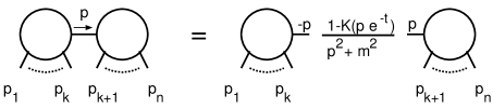
Figure 1: A 1PR graph is reduced to a product of two subgraphs. The momentum conservation implies $p\equiv p_{1}+\cdots+p_{k}=-(p_{k+1}+\cdots+p_{n})$.

We can keep reducing a 1PR graph to a multiple product of 1PI graphs and high momentum propagators with fixed momenta. Hence, our task is reduced to defining 1PI graphs.

We need a renormalization prescription to define 1PI graphs in which all loop momenta are larger than $\mathrm{e}^{t}$. We adopt an incremental procedure: given a 1PI graph, we define its value by integrating over the loop momenta scale by scale from $\mathrm{e}^{t}$ all the way to infinity.

As a preparation for this incremental procedure, let us first make the following observation. The high momentum propagator can be decomposed further as follows:

$$\frac{1-K(p\mathrm{e}^{-t})}{p^{2}+m^{2}}=\int_{t}^{\infty}dt^{\prime}\,\frac{\Delta(p\mathrm{e}^{-t^{\prime}})}{p^{2}+m^{2}}$$ (4)

where we define

$$\Delta(p\mathrm{e}^{-t})\equiv\frac{\partial}{\partial t}K(p\mathrm{e}^{-t})$$ (5)

We must use $K(0)=1$ to derive Eq. (4). The physical meaning of Eq. (4) is clear if we recall that $\Delta(p\mathrm{e}^{-t})$ is nonvanishing only for $p$ of order $\mathrm{e}^{t}$ (FIG. 2): the integrand on the right hand side of Eq. (4) gives the contribution from the momentum of order $\mathrm{e}^{t^{\prime}}$ per unit logarithmic scale $t^{\prime}$.

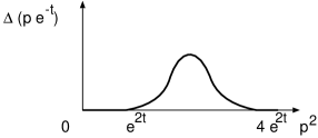
Figure 2: $\Delta(p\mathrm{e}^{-t})$ is non-vanishing only for $p^{2}$ of order $\mathrm{e}^{2t}$.

Given a 1PI diagram $G$, any of its internal lines belongs to a loop, and its momentum is integrated over. By cutting an internal line, we generate a diagram $G^{\prime}$, not necessarily 1PI, with one less number of loops but with the same number of elementary interaction vertices. In order to define the 1PI diagram recursively, we assume that the diagrams of lower order, i.e., those with less number of either loops or elementary vertices, have been defined already. We can then define the 1PI graph $G$ by

$$\mathcal{V}_{G}(-t;p_{1},\cdots,p_{n})$$ (6)

$$\equiv \sum_{G^{\prime}}\Bigg{[}\,\int_{t}^{\infty}dt^{\prime}\int_{q}\,\Delta(q\mathrm{e}^{-t^{\prime}})\Bigg{\{}\,\frac{1}{q^{2}+m^{2}}\,\mathcal{V}_{G^{\prime}}(-t^{\prime};q,-q,p_{1},\cdots,p_{n})$$

$$\qquad\qquad\qquad\qquad\qquad\quad-\Gamma_{y_{G^{\prime}}+2}\left(\frac{1}{q^{2}+m^{2}}\,\mathcal{V}_{G^{\prime}}(-t^{\prime};q,-q,p_{1},\cdots,p_{n})\right)\Bigg{\}}$$

$$-\int^{t}dt^{\prime}\,\mathrm{e}^{2t^{\prime}}\,\int_{q}\Delta(q)\cdot\Gamma_{y_{G^{\prime}}+2}\left(\frac{1}{q^{2}+m^{2}\mathrm{e}^{-2t^{\prime}}}\,\mathcal{V}_{G^{\prime}}(-t^{\prime};q\mathrm{e}^{t^{\prime}},-q\mathrm{e}^{t^{\prime}},p_{1},\cdots,p_{n})\right)\,\Bigg{]}$$

where $G^{\prime}$ is a graph obtained by cutting one internal line of $G$, and we must sum over all possible distinct choices of an internal line. We must multiply a symmetry factor of $\frac{1}{2}$ if $G^{\prime}$ cannot be distinguished from the corresponding graph with $q$ and $-q$ interchanged. This is necessary in order to avoid overcounting of the phase space. The definitions of the other unexplained symbols will be given shortly.

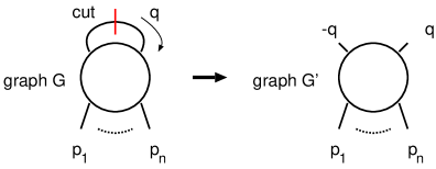
Figure 3: Any internal line of a 1PI graph belongs to a loop.

First about the scale dimension $y_{G^{\prime}}$. This is defined by the asymptotic behavior of the vertex $\mathcal{V}_{G^{\prime}}(-t)$ as $t\to\infty$:

$$\mathcal{V}_{G^{\prime}}(-t;q\mathrm{e}^{t},-q\mathrm{e}^{t},p_{1},\cdots,p_{n})\longrightarrow\text{O}\left(\mathrm{e}^{y_{G^{\prime}}t}\right)$$ (7)

where we take two momenta (loop momenta for $G$) as order $\mathrm{e}^{t}$. In a renormalizable theory, such as $\phi^{4}$, the scale dimension is determined by the number of external legs ($n+2$ for $G^{\prime}$) so that

$$y_{G^{\prime}}=4-(n+2)$$ (8)

But $y_{G^{\prime}}$ could be larger than this for non-renormalizable theories. Since the internal momenta of $\mathcal{V}_{G^{\prime}}(-t)$ are all larger than $\mathrm{e}^{t}$, we can expand $\mathcal{V}_{G^{\prime}}(-t)$ in powers of the mass $m$ and external momenta $p_{i}~{}(i=1,\cdots,n)$ with no infrared problem:

$$\mathcal{V}_{G^{\prime}}(-t;q\mathrm{e}^{t},-q\mathrm{e}^{t},p_{1},\cdots,p_{n})$$ (9)

$$= \mathrm{e}^{y_{G^{\prime}}t}~{}A_{G^{\prime}}(-t;q)+\mathrm{e}^{(y_{G^{\prime}}-2)t}~{}m^{2}B_{G^{\prime}}(-t;q)+\mathrm{e}^{(y_{G^{\prime}}-2)t}\,\frac{1}{2}\sum_{i,j}p_{i}\cdot p_{j}\,C_{G^{\prime};ij}(-t;q)+\cdots$$

where we have taken the angular average over $q$. The coefficients of the Taylor expansion, $A_{G^{\prime}}(-t;q)$, $B_{G^{\prime}}(-t;q)$, $C_{G^{\prime}}(-t;q)$, etc., are all of order $1$, or to be more precise, finite degree polynomials of $t$, to be explained later. It is crucial to observe that each power of $m$ or $p_{i}$ costs a power of $\mathrm{e}^{-t}$. This is because any loop momentum for $\mathcal{V}_{G^{\prime}}(-t)$ is at least of order $\mathrm{e}^{t}$, and the expansion is in powers of the ratio of $m$ or $p_{i}$ to $\mathrm{e}^{t}$.

We define the symbol $\Gamma_{y}$ by the finite sum of the above Taylor series up to (and including) the $y$-th order terms. For example,

$$\Gamma_{2}\,\mathcal{V}_{G^{\prime}}(-t;q\mathrm{e}^{t},-q\mathrm{e}^{t},p_{1},\cdots,p_{n})$$ (10)

$$\equiv \mathrm{e}^{y_{G^{\prime}}t}A_{G^{\prime}}(-t;q)+\mathrm{e}^{(y_{G^{\prime}}-2)t}m^{2}B_{G^{\prime}}(-t;q)+\mathrm{e}^{(y_{G^{\prime}}-2)t}\frac{1}{2}\sum_{i,j}p_{i}\cdot p_{j}C_{G^{\prime};ij}(-t;q)$$

Similarly, with $q$ rescaled by $\mathrm{e}^{-t}$, we obtain

$$\Gamma_{2}\left(\frac{1}{q^{2}+m^{2}}\mathcal{V}_{G^{\prime}}(-t;q,-q,p_{1},\cdots,p_{n})\right)$$ (11)

$$\equiv \mathrm{e}^{y_{G^{\prime}}t}\frac{1}{q^{2}}A_{G^{\prime}}(-t;q\mathrm{e}^{-t})+\mathrm{e}^{(y_{G^{\prime}}-2)t}m^{2}\left(\frac{1}{q^{2}}B_{G^{\prime}}(-t;q\mathrm{e}^{-t})-\frac{\mathrm{e}^{2t}}{q^{4}}A_{G^{\prime}}(-t;q\mathrm{e}^{-t})\right)$$

$$+\mathrm{e}^{(y_{G^{\prime}}-2)t}\frac{1}{2}\sum_{i,j}p_{i}\cdot p_{j}\frac{1}{q^{2}}C_{G^{\prime};ij}(-t;q\mathrm{e}^{-t})$$

Now that $\Gamma_{y_{G^{\prime}}+2}$ has been defined, let us look at the first two integrals of the definition (6). Rescaling the loop momentum $q$, the first loop integral is given by

$$I_{G^{\prime}}(-t^{\prime}) \equiv \int_{q}\Delta(q\mathrm{e}^{-t^{\prime}})\frac{1}{q^{2}+m^{2}}\,\mathcal{V}_{G^{\prime}}(-t^{\prime};q,-q,p_{1},\cdots,p_{n})$$ (12)

$$= \mathrm{e}^{2t^{\prime}}\int_{q}\Delta(q)\,\frac{1}{q^{2}+m^{2}\mathrm{e}^{-2t^{\prime}}}\,\mathcal{V}_{G^{\prime}}(-t^{\prime};q\mathrm{e}^{t^{\prime}},-q\mathrm{e}^{t^{\prime}},p_{1},\cdots,p_{n})$$

In the second expression, the range of the momentum integral is restricted to $q$ of order $1$, and the integral is finite, free from UV or IR divergences. Similarly, the second loop integral is given by

$$J_{G^{\prime}}(-t^{\prime}) \equiv \int_{q}\Delta(q\mathrm{e}^{-t^{\prime}})\Gamma_{y_{G^{\prime}}+2}\left(\frac{1}{q^{2}+m^{2}}\,\mathcal{V}_{G^{\prime}}(-t^{\prime};q,-q,p_{1},\cdots,p_{n})\right)$$ (13)

$$= \mathrm{e}^{2t^{\prime}}\int_{q}\Delta(q)\Gamma_{y_{G^{\prime}}+2}\left(\frac{1}{q^{2}+m^{2}\mathrm{e}^{-2t^{\prime}}}\,\mathcal{V}_{G^{\prime}}(-t^{\prime};q\mathrm{e}^{t^{\prime}},-q\mathrm{e}^{t^{\prime}},p_{1},\cdots,p_{n})\right)$$

$$= \Gamma_{y_{G^{\prime}}+2}I_{G^{\prime}}(-t^{\prime})$$

The Taylor expansion commutes with integration over $q$, and $J_{G^{\prime}}(-t^{\prime})$ gives the finite sum of the Taylor series of $I_{G^{\prime}}(-t^{\prime})$ up to order $y_{G^{\prime}}+2$.

As $t^{\prime}\to\infty$, we obtain the asymptotic behavior

$$I_{G^{\prime}}(-t^{\prime}) = \mathrm{e}^{(y_{G^{\prime}}+2)t^{\prime}}\int_{q}\frac{\Delta(q)}{q^{2}}A_{G^{\prime}}(-t^{\prime};q)+\mathrm{e}^{y_{G^{\prime}}t^{\prime}}m^{2}\int_{q}\frac{\Delta(q)}{q^{2}}\left(B_{G^{\prime}}(-t^{\prime};q)-\frac{A_{G^{\prime}}(-t^{\prime};q)}{q^{2}}\right)$$ (14)

$$+\mathrm{e}^{y_{G^{\prime}}t^{\prime}}\frac{1}{2}\sum_{i,j}p_{i}\cdot p_{j}\int_{q}\frac{\Delta(q)}{q^{2}}C_{G^{\prime};ij}(-t^{\prime};q)+\cdots$$

Each power of $m$ or $p_{i}$ costs a power of $\mathrm{e}^{-t^{\prime}}$. Hence, the integral $J_{G^{\prime}}(-t^{\prime})$ corresponds only to the part of $I_{G^{\prime}}(-t^{\prime})$ that does not vanish in the limit $t^{\prime}\to\infty$. Therefore, we obtain

$$I_{G^{\prime}}(-t^{\prime})-J_{G^{\prime}}(-t^{\prime})=\mathrm{O}\left(\mathrm{e}^{-t^{\prime}}{t^{\prime}}^{k}\right)$$ (15)

where $k$ is an integer. This implies that we can integrate the difference $I_{G^{\prime}}(-t^{\prime})-J_{G^{\prime}}(-t^{\prime})$ over $t^{\prime}$ all the way to $\infty$. Therefore, the integral

$$\int_{t}^{\infty}dt^{\prime}\,\left(I_{G^{\prime}}(-t^{\prime})-J_{G^{\prime}}(-t^{\prime})\right)$$ (16)

is free of UV divergences, and well defined.

The finite counterterms, given by the last integral in Eq. (6), are introduced to cancel the $t$ dependence of the UV subtraction $J_{G^{\prime}}(-t)$. Let us call the finite counterterms by $F_{G^{\prime}}(-t)$. We want $F_{G^{\prime}}(-t)$ to satisfy

$$\frac{\partial}{\partial t}F_{G^{\prime}}(-t)=-J_{G^{\prime}}(-t)$$ (17)

so that

$$-\frac{\partial}{\partial t}\left[\int_{t}^{\infty}dt^{\prime}\,\left(I_{G^{\prime}}(-t^{\prime})-J_{G^{\prime}}(-t^{\prime})\right)+F_{G^{\prime}}(-t)\right]=I_{G^{\prime}}(-t)$$ (18)

Eq. (17) is formally solved by

$$F_{G^{\prime}}(-t)=-\int^{t}dt^{\prime}\,J_{G^{\prime}}(-t^{\prime})$$ (19)

We recall that the terms of $J_{G^{\prime}}(-t^{\prime})$ have the form $\mathrm{e}^{yt^{\prime}}t^{\prime k}$ where $y\geq 0$ and $k$ is a non-negative integer. To make the definition (19) precise, we need to specify what we mean by the finite integral of $\mathrm{e}^{yt^{\prime}}t^{\prime k}$.

There is no unique choice for the finite integrals. Any specification is a convention free of any physical meaning. We find it most convenient to introduce our version of a minimal subtraction scheme by using the following convention: for $y>0$

$$\int^{t}dt^{\prime}\,\mathrm{e}^{yt^{\prime}}{t^{\prime}}^{k}\equiv\mathrm{e}^{yt}P_{y,k}(t)$$ (20)

where $P_{y,k}$ is the $k$-th degree polynomial of $t$ defined uniquely by

$$\frac{d}{dt}\left(\mathrm{e}^{yt}P_{y,k}(t)\right)=\mathrm{e}^{yt}t^{k}$$ (21)

and for $y=0$

$$\int^{t}dt^{\prime}\,{t^{\prime}}^{k}\equiv\int_{0}^{t}dt^{\prime}\,{t^{\prime}}^{k}=\frac{t^{k+1}}{k+1}$$ (22)

With this convention, Eq. (19) defines the finite counterterms.

To summarize, and using a more symbolic notation than Eq. (6), we define

$$\mathcal{V}_{G}(-t;p_{1},\cdots,p_{n})=\sum_{G^{\prime}}\left[\int_{t}^{\infty}dt^{\prime}\,(I_{G^{\prime}}(-t^{\prime})-J_{G^{\prime}}(-t^{\prime}))+F_{G^{\prime}}(-t)\right]$$ (23)

where the summation is over all distinct choices of an internal line of $G$, $I_{G^{\prime}}$ is given by Eq. (12), $J_{G^{\prime}}$ by Eq. (13), and $F_{G^{\prime}}$ by Eq. (19) and the convention (20, 21, 22).

The prescription (6) or (23) is reminiscent of the BPHZ scheme in which Taylor expansions in powers of external momenta are used. There is a significant difference between the two schemes, however. In BPHZ the whole vertex functions are expanded, but here only the high energy part of the vertex functions are expanded. This is why our prescription works for the massless theory, but not BPHZ.

A remark is in order. We have mentioned that the Taylor coefficients of $\mathcal{V}_{G^{\prime}}(-t)$, i.e., $A_{G^{\prime}}(-t),B_{G^{\prime}}(-t),C_{G^{\prime}}(-t)$, etc., are finite polynomials of $t$. We have also mentioned that $J_{G^{\prime}}(-t)$ consists of terms of the form $\mathrm{e}^{yt}t^{k}$. These two statements are the same. To prove either statement, we notice that the definition (23) implies the asymptotic behavior

$$\mathcal{V}_{G}(-t)\longrightarrow\sum_{G^{\prime}}F_{G^{\prime}}(-t)$$ (24)

since

$$\int_{t}^{\infty}dt^{\prime}\left(I_{G^{\prime}}(-t^{\prime})-J_{G^{\prime}}(-t^{\prime})\right)\longrightarrow 0$$ (25)

as $t\to\infty$. Now, $F_{G^{\prime}}(-t)$ is a finite integral (over $t$) of $J_{G^{\prime}}(-t)$, which is determined by the asymptotic behavior of $\mathcal{V}_{G^{\prime}}(-t)$. Therefore, the asymptotic behavior of $\mathcal{V}_{G}(-t)$ is determined by that of $\mathcal{V}_{G^{\prime}}(-t)$. Hence, it is not hard to see that we can prove the above mentioned $t$-dependence of $J_{G^{\prime}}(-t)$ by mathematical induction on the order (number of loops plus elementary vertices) of graphs.

As an example, we take the four-dimensional $\phi^{4}$ theory. (See FIG. 4.)

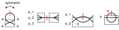
Figure 4: Examples from $\phi^{4}$ theory

Let $(-\lambda)$ be the elementary vertex. Then, the one-loop self energy is given by

$$\mathcal{V}_{2}^{(1)}(-t) = (-\lambda)\Bigg{[}\,\int_{t}^{\infty}dt^{\prime}\frac{1}{2}\int_{q}\Delta(q\mathrm{e}^{-t^{\prime}})\left(\frac{1}{q^{2}+m^{2}}-\frac{1}{q^{2}}+\frac{m^{2}}{q^{4}}\right)$$ (26)

$$\quad-\frac{\mathrm{e}^{2t}}{4}\int_{q}\frac{\Delta(q)}{q^{2}}+\frac{m^{2}}{2}t\int_{q}\frac{\Delta(q)}{q^{4}}\,\Bigg{]}$$

which is independent of external momentum. The symmetry factor $\frac{1}{2}$ is necessary, since the cut graph with external momenta $q,-q$ is the same as that with $-q,q$.

At order $\lambda^{2}$, the six-point vertex is given by 1PR graphs, and we obtain

$$\mathcal{V}_{6}(-t;p_{1},\cdots,p_{6})=(-\lambda)^{2}\left[\frac{1-K((p_{1}+p_{2}+p_{3})\mathrm{e}^{-t})}{(p_{1}+p_{2}+p_{3})^{2}+m^{2}}+\text{9~{}permutations}\right]$$ (27)

The one-loop four-point vertex in the s-channel is given by

$$\mathcal{V}_{4\mathrm{s}}^{(2)}(-t;p_{1},\cdots,p_{4})$$ (28)

$$= (-\lambda)^{2}\Bigg{[}\int_{t}^{\infty}dt^{\prime}\int_{q}\,\Delta(q\mathrm{e}^{-t^{\prime}})\Bigg{\{}\frac{1}{q^{2}+m^{2}}\,\frac{1-K((q+p_{1}+p_{2})\mathrm{e}^{-t^{\prime}})}{(q+p_{1}+p_{2})^{2}+m^{2}}-\frac{1-K(q\mathrm{e}^{-t^{\prime}})}{q^{4}}\Bigg{\}}$$

$$\qquad\quad-t\int_{q}\frac{\Delta(q)(1-K(q))}{q^{4}}\>\Bigg{]}$$

To compute the two-point vertex $\mathcal{V}_{2}$ at order $\lambda^{2}$, we need to expand $\mathcal{V}_{4\mathrm{s}}^{(2)}$ in external momentum $p$ and squared mass:

$$\Gamma_{2}\mathcal{V}_{4\mathrm{s}}^{(2)}(-t;q\mathrm{e}^{t},p,-q\mathrm{e}^{t},-p)=A_{4}(-t;q)+\mathrm{e}^{-2t}\left(m^{2}B_{4}(-t;q)+p^{2}C_{4}(-t;q)\right)$$ (29)

where $A_{4}(-t;q),B_{4}(-t;q),C_{4}(-t;q)$ are at most linear in $t$ for fixed $q$. Then we obtain

$$\mathcal{V}_{2}^{(2)}(-t;p,-p)$$ (30)

$$= (-\lambda)^{2}\Bigg{[}\int_{t}^{\infty}dt^{\prime}\,\mathrm{e}^{2t^{\prime}}\int_{q}\Delta(q)\Bigg{\{}\frac{1}{q^{2}+m^{2}\mathrm{e}^{-2t^{\prime}}}\mathcal{V}_{4\mathrm{s}}^{(2)}(-t^{\prime};q\mathrm{e}^{t^{\prime}},p,-q\mathrm{e}^{t^{\prime}},-p)$$

$$-\frac{1}{q^{2}}\left(1-\frac{\mathrm{e}^{-2t^{\prime}}m^{2}}{q^{2}}\right)A_{4}(-t^{\prime};q)-\frac{\mathrm{e}^{-2t^{\prime}}m^{2}}{q^{2}}B_{4}(-t^{\prime};q)-\frac{\mathrm{e}^{-2t^{\prime}}p^{2}}{q^{2}}C_{4}(-t^{\prime};q)\Bigg{\}}$$

$$-\int^{t}dt^{\prime}\,\mathrm{e}^{2t^{\prime}}\int_{q}\frac{\Delta(q)}{q^{2}}A_{4}(-t^{\prime};q)-m^{2}\int_{0}^{t}dt^{\prime}\,\int_{q}\,{\Delta(q)}\left(\frac{B_{4}(-t^{\prime};q)}{q^{2}}-\frac{A_{4}(-t^{\prime};q)}{q^{4}}\right)$$

$$\qquad-p^{2}\int_{0}^{t}dt^{\prime}\,\int_{q}\frac{\Delta(q)}{q^{2}}C_{4}(-t^{\prime};q)\,\Bigg{]}$$

We will give more explicit expressions of $A_{4},B_{4},C_{4}$ in Appendix A.

So far we have only described the prescription. A justification is in order. The recursive definition (6) is constructed so that for a 1PI graph $G$, we find

$$-\frac{\partial}{\partial t}\mathcal{V}_{G}(-t;p_{1},\cdots,p_{n})=\int_{q}\frac{\Delta(q\mathrm{e}^{-t})}{q^{2}+m^{2}}\,\sum_{G^{\prime}}\mathcal{V}_{G^{\prime}}(-t;q,-q,p_{1},\cdots,p_{n})$$ (31)

Recall Eq. (17): the finite subtraction $F_{G^{\prime}}(-t)$ has been introduced to cancel the $t$-dependence of the UV subtraction $J_{G^{\prime}}(-t)$.

Now, summing over all Feynman diagrams with $n$ external lines, including both 1PR and 1PI diagrams, we obtain the $n$-point vertex:

$$\mathcal{V}_{n}(-t;p_{1},\cdots,p_{n})\equiv\sum_{G~{}\mathrm{with~{}}n~{}\mathrm{legs}}\mathcal{V}_{G}(-t;p_{1},\cdots,p_{n})$$ (32)

Eq. (31) and the rule for 1PR graphs imply

$$-\frac{\partial}{\partial t}\mathcal{V}_{n}(-t;p_{1},\cdots,p_{n})$$ (33)

$$= \sum_{k=0}^{\left[\frac{n}{2}\right]}\sum_{\mathrm{partitions}~{}\sigma}\mathcal{V}_{k+1}(-t;p_{\sigma(1)},\cdots,p_{\sigma(k)},-(p_{\sigma(1)}+\cdots+p_{\sigma(k)}))$$

$$\quad\times\frac{\Delta(p_{\sigma(1)}+\cdots+p_{\sigma(k)})}{(p_{\sigma(1)}+\cdots+p_{\sigma(k)})^{2}+m^{2}}\,\mathcal{V}_{n-k+1}(-t;p_{\sigma(k+1)},\cdots,p_{\sigma(n)},p_{\sigma(1)}+\cdots+p_{\sigma(k)})$$

$$+\frac{1}{2}\int_{q}\frac{\Delta(q\mathrm{e}^{-t})}{q^{2}+m^{2}}\,\mathcal{V}_{n+2}(-t;q,-q,p_{1},\cdots,p_{n})$$

where the sum is over all possible partitions of $n$ external momenta into two groups. This is the exact renormalization group (ERG) differential equation of Wilson Wilson and Kogut (1974) in the form given by Polchinski.Polchinski (1984) The exact renormalization group equation guarantees that the Green functions are independent of the choice of the scale parameter $t$. The prescription (6) can then be understood as the diagrammatic solution of the exact RG differential equation (33). Hence, the exact renormalization group justifies our diagrammatic prescription (6).

Actually our prescription is more than a diagrammatic solution to the ERG differential equation. A new formulation of the ERG in terms of integral equations has been derived recently in Ref. Sonoda (2003). Our renormalization prescription is a solution of the integral equations in terms of Feynman diagrams.

A generalization to fermions is straightforward. All we need to do is to replace the propagator by

$$\frac{1}{\hbox{$p$\kern-5.0pt\raise 1.29167pt\hbox{/}}+im}\longrightarrow\frac{K(p)}{\hbox{$p$\kern-5.0pt\raise 1.29167pt\hbox{/}}+im}$$ (34)

A classical test of a renormalization scheme is the derivation of the axial anomaly. (See FIG. 5.) For the massless fermion, we obtain the following amplitude:

$$\mathcal{T}_{\mu\alpha\beta}(k_{1},k_{2})=-\int_{t}^{\infty}dt^{\prime}\int_{q}\,\mathrm{Sp}~{}\gamma_{5}\gamma_{\mu}\frac{1}{\hbox{$q$\kern-5.0pt\raise 1.29167pt\hbox{/}}}\gamma_{\alpha}\frac{1}{\hbox{$q$\kern-5.0pt\raise 1.29167pt\hbox{/}}+\hbox{$k$\kern-5.0pt\raise 1.29167pt\hbox{/}}_{1}}\gamma_{\beta}\frac{1}{\hbox{$q$\kern-5.0pt\raise 1.29167pt\hbox{/}}+\hbox{$k$\kern-5.0pt\raise 1.29167pt\hbox{/}}_{1}+\hbox{$k$\kern-5.0pt\raise 1.29167pt\hbox{/}}_{2}}$$ (35)

$$\times\Bigg{[}\,\Delta(q\mathrm{e}^{-t^{\prime}})\{1-K((q+k_{1})\mathrm{e}^{-t^{\prime}})\}\{1-K((q+k_{1}+k_{2})\mathrm{e}^{-t^{\prime}})\}$$

$$\quad+\{1-K(q\mathrm{e}^{-t^{\prime}})\}\Delta((q+k_{1})\mathrm{e}^{-t^{\prime}})\{1-K((q+k_{1}+k_{2})\mathrm{e}^{-t^{\prime}})\}$$

$$\quad+\{1-K(q\mathrm{e}^{-t^{\prime}})\}\{1-K((q+k_{1})\mathrm{e}^{-t^{\prime}})\}\Delta((q+k_{1}+k_{2})\mathrm{e}^{-t^{\prime}})\,\Bigg{]}$$

$$- \int_{q}\mathrm{Sp}~{}\gamma_{5}\gamma_{\mu}\frac{1}{\hbox{$q$\kern-5.0pt\raise 1.29167pt\hbox{/}}}\gamma_{\alpha}\frac{1}{\hbox{$q$\kern-5.0pt\raise 1.29167pt\hbox{/}}+\hbox{$k$\kern-5.0pt\raise 1.29167pt\hbox{/}}_{1}}\gamma_{\beta}\frac{1}{\hbox{$q$\kern-5.0pt\raise 1.29167pt\hbox{/}}+\hbox{$k$\kern-5.0pt\raise 1.29167pt\hbox{/}}_{1}+\hbox{$k$\kern-5.0pt\raise 1.29167pt\hbox{/}}_{2}}$$

$$\times\left[1-\{1-K(q\mathrm{e}^{-t})\}\{1-K((q+k_{1})\mathrm{e}^{-t})\}\{1-K((q+k_{1}+k_{2})\mathrm{e}^{-t})\}\right]$$

$$- (\mbox{the above two integrals with }k_{1},\alpha\leftrightarrow k_{2},\beta)+c\,\epsilon_{\mu\alpha\beta\gamma}(k_{1}-k_{2})_{\gamma}$$

where $c$ is a constant coefficient of the finite counterterm. This is independent of the logarithmic scale parameter $t$.

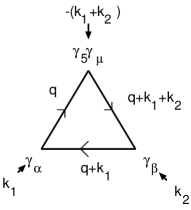
Figure 5: Triangle anomaly

Potentially the integrand of the $t^{\prime}$ integral behaves as $\mathrm{e}^{t^{\prime}}$ for large $t^{\prime}$, but we can check its absence. In fact the integrand behaves as $\mathrm{e}^{-t^{\prime}}$, and no UV subtraction is necessary. The $t$-dependence of the first integral cancels that of the second, and the whole right-hand side is independent of $t$. We note that the loop momentum $q$ can be shifted; a potential UV divergence come from the integral over $t^{\prime}$, not $q$.

In Appendix B we will show the following two:

1. For the current conservation

   $$(k_{1})_{\alpha}\mathcal{T}_{\mu\alpha\beta}(k_{1},k_{2})=0$$ (36)

   we must choose

   $$c=-\frac{8}{3(4\pi)^{2}}$$ (37)

2. The axial anomaly is given by

   $$(k_{1}+k_{2})_{\mu}\mathcal{T}_{\mu\alpha\beta}(k_{1},k_{2})=\frac{8}{(4\pi)^{2}}\epsilon_{\alpha\beta\gamma\delta}(k_{1})_{\gamma}(k_{2})_{\delta}$$ (38)

Hence, our prescription passes the classical test.

In conclusion we have given a new renormalization prescription of Feynman diagrams. The prescription gives a refinement of the naive momentum cutoff regularization, and it resembles both BPHZ and MS with dimensional regularization. The prescription gives manifestly UV finite expressions like the BPHZ scheme, and it is mass independent and works for massless theories like the MS scheme with dimensional regularization. The exact renormalization group of Wilson validates our renormalization prescription.

Gauge symmetry and non-linearly realized symmetry are not manifest under our new renormalization scheme, and we must introduce additional finite counterterms to enforce a symmetry. With the help of the exact renormalization group, however, the analysis of the relevant Ward identities to all orders in perturbation theory becomes straightforward.Sonoda (a)

Appendix A More details on the two-loop self-energy

Similar calculations can be found in Ref. Sonoda (b). We omit the factor of $(-\lambda)^{2}$ in the rest of the calculations. From Eqs. (28) we obtain

$$\mathcal{V}_{4\mathrm{s}}^{(2)}(-t;q\mathrm{e}^{t},p,-q\mathrm{e}^{t},-p)$$ (39)

$$= \int_{0}^{\infty}dt^{\prime}\int_{q^{\prime}}\Delta(q^{\prime}\mathrm{e}^{-t^{\prime}})\left\{\frac{1}{q^{\prime 2}+m^{2}\mathrm{e}^{-2t}}\cdot\frac{1-K((q^{\prime}+q+p\mathrm{e}^{-t})\mathrm{e}^{-t^{\prime}})}{(q^{\prime}+q+p\mathrm{e}^{-t})^{2}+m^{2}\mathrm{e}^{-2t}}-\frac{1-K(q^{\prime}\mathrm{e}^{-t^{\prime}})}{q^{\prime 4}}\right\}$$

$$\quad-t\int_{q^{\prime}}\frac{\Delta(q^{\prime})(1-K(q^{\prime}))}{q^{\prime 4}}$$

Expanding this in powers of $m^{2}$ and $p^{2}$, we obtain

$$A_{4}(-t;q)=\int_{0}^{\infty}dt^{\prime}\int_{q^{\prime}}\frac{\Delta(q^{\prime}\mathrm{e}^{-t^{\prime}})}{q^{\prime 2}}\left(\frac{1-K((q^{\prime}+q)\mathrm{e}^{-t^{\prime}})}{(q^{\prime}+q)^{2}}-\frac{1-K(q^{\prime}\mathrm{e}^{-t^{\prime}})}{q^{\prime 2}}\right)$$

$$\qquad\qquad-t\int_{q^{\prime}}\frac{\Delta(q^{\prime})(1-K(q^{\prime}))}{{q^{\prime}}^{4}}$$

$$B_{4}(-t;q)$$

$$= -\int_{0}^{\infty}dt^{\prime}\int_{q^{\prime}}\Delta(q^{\prime}\mathrm{e}^{-t^{\prime}})(1-K((q^{\prime}+q)\mathrm{e}^{-t^{\prime}}))\left(\frac{1}{{q^{\prime}}^{4}(q^{\prime}+q)^{2}}+\frac{1}{q^{\prime 2}(q^{\prime}+q)^{4}}\right)$$ (42)

$$C_{4}(-t;q)=\int_{0}^{\infty}dt^{\prime}\frac{\partial}{\partial p^{2}}\left[\int_{q^{\prime}}\frac{\Delta(q^{\prime}\mathrm{e}^{-t^{\prime}})(1-K((q^{\prime}+q+p)\mathrm{e}^{-t^{\prime}}))}{{q^{\prime}}^{2}}\right]_{p^{2}=0}$$

This shows manifestly that $A_{4}(-t;q)$ is at most linear in $t$, and that both $B_{4}(-t;q)$ and $C_{4}(-t;q)$ are independent of $t$. We will write them as $B_{4}(q)$ and $C_{4}(q)$, respectively.

We can simplify the expression for $B_{4}$ further by integrating over $t^{\prime}$ first:

$$B_{4}(q) = \int_{0}^{\infty}dt^{\prime}\frac{\partial}{\partial t^{\prime}}\int_{q^{\prime}}\frac{(1-K(q^{\prime}\mathrm{e}^{-t^{\prime}}))(1-K((q^{\prime}+q)\mathrm{e}^{-t^{\prime}}))}{{q^{\prime}}^{4}(q^{\prime}+q)^{2}}$$ (43)

$$= -\int_{q^{\prime}}\frac{(1-K(q^{\prime}))(1-K((q^{\prime}+q)))}{{q^{\prime}}^{4}(q^{\prime}+q)^{2}}$$

This integral is UV (and IR) finite.

Hence, using the above results we can compute the finite counterterms:

(1) $$\int^{t}dt^{\prime}\,\mathrm{e}^{2t^{\prime}}\int_{q}\frac{\Delta(q)}{q^{2}}A_{4}(-t^{\prime};q)$$

$$= \frac{\mathrm{e}^{2t}}{2}\int_{q}\frac{\Delta(q)}{q^{2}}\int_{0}^{\infty}dt^{\prime}\int_{q^{\prime}}\frac{\Delta(q^{\prime}\mathrm{e}^{-t^{\prime}})}{{q^{\prime}}^{2}}\left(\frac{1-K((q^{\prime}+q)e^{-t^{\prime}})}{(q^{\prime}+q)^{2}}-\frac{1-K(q^{\prime}\mathrm{e}^{-t^{\prime}})}{{q^{\prime}}^{2}}\right)$$

$$\qquad\qquad-\mathrm{e}^{2t}\left(\frac{t}{2}-\frac{1}{4}\right)\int_{q}\frac{\Delta(q)}{q^{2}}\int_{q^{\prime}}\frac{\Delta(q^{\prime})(1-K(q^{\prime}))}{{q^{\prime}}^{4}},$$

(2) $$\int_{0}^{t}dt^{\prime}\,\int_{q}\Delta(q)\left(\frac{B_{4}(q)}{q^{2}}-\frac{A_{4}(-t^{\prime};q)}{q^{4}}\right)$$

$$= -t\int_{q}\frac{\Delta(q)}{q^{2}}\int_{q^{\prime}}\frac{(1-K(q))(1-K(q^{\prime}+q))}{{q^{\prime}}^{4}(q^{\prime}+q)^{2}}$$

$$-t\int_{q}\frac{\Delta(q)}{q^{4}}\int_{0}^{\infty}dt^{\prime}\int_{q^{\prime}}\frac{\Delta(q^{\prime}\mathrm{e}^{-t^{\prime}})}{{q^{\prime}}^{2}}\left(\frac{1-K((q^{\prime}+q)e^{-t^{\prime}})}{(q^{\prime}+q)^{2}}-\frac{1-K(q^{\prime}\mathrm{e}^{-t^{\prime}})}{{q^{\prime}}^{2}}\right)$$

$$+\frac{t^{2}}{2}\int_{q}\frac{\Delta(q)}{q^{4}}\int_{q^{\prime}}\frac{\Delta(q^{\prime})(1-K(q^{\prime}))}{{q^{\prime}}^{4}},$$

(3) $$\int_{0}^{t}dt^{\prime}\,\int_{q}\frac{\Delta(q)}{q^{2}}C_{4}(q)$$

$$= t\int_{0}^{\infty}dt^{\prime}\int_{q}\frac{\Delta(q)}{q^{2}}\frac{\partial}{\partial p^{2}}\left\{\int_{q^{\prime}}\frac{\Delta(q^{\prime}\mathrm{e}^{-t^{\prime}})}{{q^{\prime}}^{2}}\frac{1-K((q^{\prime}+q+p)\mathrm{e}^{-t^{\prime}})}{(q^{\prime}+q+p)^{2}}\right\}_{p=0}$$

$$= t\int_{0}^{\infty}dt^{\prime}\int_{q}\frac{\Delta(q\mathrm{e}^{t^{\prime}})}{q^{2}}\int_{q^{\prime}}\frac{\Delta(q^{\prime})}{{q^{\prime}}^{2}}\frac{d^{2}K(q^{\prime}+q)}{(d(q^{\prime}+q)^{2})^{2}}$$

$$= t\int_{q}\frac{K(q)}{q^{2}}\int_{q^{\prime}}\frac{\Delta(q^{\prime})}{{q^{\prime}}^{2}}\frac{d^{2}K(q^{\prime}+q)}{(d(q^{\prime}+q)^{2})^{2}}$$ (46)

Some of the integrals have values independent of the choice of $K$, but we will not discuss it here.

Appendix B Derivation of the axial anomaly

We give details of the calculation of the axial anomaly in this appendix. We first define

$$T_{1,\mu\alpha\beta}(-t;k_{1},k_{2})\equiv-\int_{t}^{\infty}dt^{\prime}\int_{q}\,\mathrm{Sp}~{}\gamma_{5}\gamma_{\mu}\frac{1}{\hbox{$q$\kern-5.0pt\raise 1.29167pt\hbox{/}}}\gamma_{\alpha}\frac{1}{\hbox{$q$\kern-5.0pt\raise 1.29167pt\hbox{/}}+\hbox{$k$\kern-5.0pt\raise 1.29167pt\hbox{/}}_{1}}\gamma_{\beta}\frac{1}{\hbox{$q$\kern-5.0pt\raise 1.29167pt\hbox{/}}+\hbox{$k$\kern-5.0pt\raise 1.29167pt\hbox{/}}_{1}+\hbox{$k$\kern-5.0pt\raise 1.29167pt\hbox{/}}_{2}}$$

$$\times\Bigg{[}\,\Delta(q\mathrm{e}^{-t^{\prime}})\{1-K((q+k_{1})\mathrm{e}^{-t^{\prime}})\}\{1-K((q+k_{1}+k_{2})\mathrm{e}^{-t^{\prime}})\}$$

$$\quad+\{1-K(q\mathrm{e}^{-t^{\prime}})\}\Delta((q+k_{1})\mathrm{e}^{-t^{\prime}})\{1-K((q+k_{1}+k_{2})\mathrm{e}^{-t^{\prime}})\}$$

$$\quad+\{1-K(q\mathrm{e}^{-t^{\prime}})\}\{1-K((q+k_{1})\mathrm{e}^{-t^{\prime}})\}\Delta((q+k_{1}+k_{2})\mathrm{e}^{-t^{\prime}})\,\Bigg{]}$$ (47)

and

$$T_{2,\mu\alpha\beta}(-t;k_{1},k_{2})\equiv-\int_{q}\,\mathrm{Sp}~{}\gamma_{5}\gamma_{\mu}\frac{1}{\hbox{$q$\kern-5.0pt\raise 1.29167pt\hbox{/}}}\gamma_{\alpha}\frac{1}{\hbox{$q$\kern-5.0pt\raise 1.29167pt\hbox{/}}+\hbox{$k$\kern-5.0pt\raise 1.29167pt\hbox{/}}_{1}}\gamma_{\beta}\frac{1}{\hbox{$q$\kern-5.0pt\raise 1.29167pt\hbox{/}}+\hbox{$k$\kern-5.0pt\raise 1.29167pt\hbox{/}}_{1}+\hbox{$k$\kern-5.0pt\raise 1.29167pt\hbox{/}}_{2}}$$

$$\times\left[1-\{1-K(q\mathrm{e}^{-t})\}\{1-K((q+k_{1})\mathrm{e}^{-t})\}\{1-K((q+k_{1}+k_{2})\mathrm{e}^{-t})\}\right]$$ (48)

so that

$$\mathcal{T}_{\mu\alpha\beta}(k_{1},k_{2}) = T_{1,\mu\alpha\beta}(-t;k_{1},k_{2})+T_{2,\mu\alpha\beta}(-t;k_{1},k_{2})$$ (49)

$$+T_{1,\mu\beta\alpha}(-t;k_{2},k_{1})+T_{2,\mu\beta\alpha}(-t;k_{2},k_{1})+c\,\epsilon_{\mu\alpha\beta\gamma}(k_{1}-k_{2})_{\gamma}$$

The $t$-dependence of $T_{1}$ cancels that of $T_{2}$, and $\mathcal{T}$ is independent of $t$.

To compute $(k_{1}+k_{2})_{\mu}T_{1,\mu\alpha\beta}(k_{1},k_{2})$, we use the well-known trick:

$$\hbox{$k$\kern-5.0pt\raise 1.29167pt\hbox{/}}_{1}+\hbox{$k$\kern-5.0pt\raise 1.29167pt\hbox{/}}_{2}=\hbox{$q$\kern-5.0pt\raise 1.29167pt\hbox{/}}-(\hbox{$q$\kern-5.0pt\raise 1.29167pt\hbox{/}}-\hbox{$k$\kern-5.0pt\raise 1.29167pt\hbox{/}}_{1}-\hbox{$k$\kern-5.0pt\raise 1.29167pt\hbox{/}}_{2})$$ (50)

We also use the identity

$$\Delta(q\mathrm{e}^{-t^{\prime}})\{1-K((q+k_{1})\mathrm{e}^{-t^{\prime}})\}\{1-K((q+k_{1}+k_{2})\mathrm{e}^{-t^{\prime}})\}$$ (51)

$$\quad+\{1-K(q\mathrm{e}^{-t^{\prime}})\}\Delta((q+k_{1})\mathrm{e}^{-t^{\prime}})\{1-K((q+k_{1}+k_{2})\mathrm{e}^{-t^{\prime}})\}$$

$$\quad+\{1-K(q\mathrm{e}^{-t^{\prime}})\}\{1-K((q+k_{1})\mathrm{e}^{-t^{\prime}})\}\Delta((q+k_{1}+k_{2})\mathrm{e}^{-t^{\prime}})$$

$$= \frac{\partial}{\partial t^{\prime}}\left[1-\{1-K(q\mathrm{e}^{-t^{\prime}})\}\{1-K((q+k_{1})\mathrm{e}^{-t^{\prime}})\}\{1-K((q+k_{1}+k_{2})\mathrm{e}^{-t^{\prime}})\}\right]$$

We then obtain

$$(k_{1}+k_{2})_{\mu}T_{1,\mu\alpha\beta}(-t;k_{1},k_{2})$$ (52)

$$= -\int_{t}^{\infty}dt^{\prime}\frac{\partial}{\partial t^{\prime}}\int_{q}\left(\mathrm{Sp}~{}\gamma_{5}\gamma_{\alpha}\frac{1}{\hbox{$q$\kern-5.0pt\raise 1.29167pt\hbox{/}}-\hbox{$k$\kern-5.0pt\raise 1.29167pt\hbox{/}}_{1}}\gamma_{\beta}\frac{1}{\hbox{$q$\kern-5.0pt\raise 1.29167pt\hbox{/}}-\hbox{$k$\kern-5.0pt\raise 1.29167pt\hbox{/}}_{1}-\hbox{$k$\kern-5.0pt\raise 1.29167pt\hbox{/}}_{2}}+\mathrm{Sp}~{}\gamma_{5}\frac{1}{\hbox{$q$\kern-5.0pt\raise 1.29167pt\hbox{/}}}\gamma_{\alpha}\frac{1}{\hbox{$q$\kern-5.0pt\raise 1.29167pt\hbox{/}}-\hbox{$k$\kern-5.0pt\raise 1.29167pt\hbox{/}}_{1}}\gamma_{\beta}\right)$$

$$\times\left[1-\{1-K(q\mathrm{e}^{-t^{\prime}})\}\{1-K((q+k_{1})\mathrm{e}^{-t^{\prime}})\}\{1-K((q+k_{1}+k_{2})\mathrm{e}^{-t^{\prime}})\}\right]$$

For the first trace, we replace $q$ by $-q+k_{1}+k_{2}$. Then, we get

$$(k_{1}+k_{2})_{\mu}T_{1,\mu\alpha\beta}(-t;k_{1},k_{2})$$ (53)

$$= -\int_{t}^{\infty}\frac{\partial}{\partial t^{\prime}}\int_{q}\Bigg{[}\left\{1-(1-K(q\mathrm{e}^{-t^{\prime}}))(1-K((q+k_{1})\mathrm{e}^{-t^{\prime}}))(1-K((q+k_{1}+k_{2})\mathrm{e}^{-t^{\prime}}))\right\}$$

$$\qquad\qquad\times\mathrm{Sp}~{}\gamma_{5}\frac{1}{\hbox{$q$\kern-5.0pt\raise 1.29167pt\hbox{/}}}\gamma_{\alpha}\frac{1}{\hbox{$q$\kern-5.0pt\raise 1.29167pt\hbox{/}}-\hbox{$k$\kern-5.0pt\raise 1.29167pt\hbox{/}}_{1}}\gamma_{\beta}\quad-(k_{1}\leftrightarrow k_{2})\,\Bigg{]}$$

Hence,

$$(k_{1}+k_{2})_{\mu}T_{1,\mu\alpha\beta}(-t;k_{1},k_{2})$$ (54)

$$= -\lim_{T\to\infty}\int_{q}\Bigg{[}\mathrm{e}^{2T}\left\{1-(1-K(q))(1-K(q-k_{1}\mathrm{e}^{-T}))(1-K(q-(k_{1}+k_{2})\mathrm{e}^{-T}))\right\}$$

$$\times\mathrm{Sp}~{}\gamma_{5}\frac{1}{\hbox{$q$\kern-5.0pt\raise 1.29167pt\hbox{/}}}\gamma_{\alpha}\frac{1}{\hbox{$q$\kern-5.0pt\raise 1.29167pt\hbox{/}}-\hbox{$k$\kern-5.0pt\raise 1.29167pt\hbox{/}}_{1}\mathrm{e}^{-T}}\gamma_{\beta}\quad-(k_{1}\leftrightarrow k_{2})\Bigg{]}\quad-(k_{1}+k_{2})_{\mu}T_{2,\mu\alpha\beta}(-t;k_{1},k_{2})$$

Therefore, we obtain

$$(k_{1}+k_{2})_{\mu}\left(T_{1,\mu\alpha\beta}(-t;k_{1},k_{2})+T_{2,\mu\alpha\beta}(-t;k_{1},k_{2})\right)$$ (55)

$$= -\lim_{T\to\infty}\int_{q}\Bigg{[}\mathrm{e}^{2T}\left\{1-(1-K(q))(1-K(q-k_{1}\mathrm{e}^{-T}))(1-K(q-(k_{1}+k_{2})\mathrm{e}^{-T}))\right\}$$

$$\times\mathrm{Sp}~{}\gamma_{5}\frac{1}{\hbox{$q$\kern-5.0pt\raise 1.29167pt\hbox{/}}}\gamma_{\alpha}\frac{1}{\hbox{$q$\kern-5.0pt\raise 1.29167pt\hbox{/}}-\hbox{$k$\kern-5.0pt\raise 1.29167pt\hbox{/}}_{1}\mathrm{e}^{-T}}\gamma_{\beta}\quad-(k_{1}\leftrightarrow k_{2})\Bigg{]}$$

This expression shows clearly that the anomaly comes from the UV limit. Computing the trace

$$\mathrm{Sp}~{}\gamma_{5}\frac{1}{\hbox{$q$\kern-5.0pt\raise 1.29167pt\hbox{/}}}\gamma_{\alpha}\frac{1}{\hbox{$q$\kern-5.0pt\raise 1.29167pt\hbox{/}}-\hbox{$k$\kern-5.0pt\raise 1.29167pt\hbox{/}}_{1}\mathrm{e}^{-T}}\gamma_{\beta}\\ =-\frac{4\mathrm{e}^{-T}}{q^{2}(q-k_{1}\mathrm{e}^{-T})^{2}}\epsilon_{\mu\alpha\nu\beta}q_{\mu}k_{1\nu}$$

we obtain

$$(k_{1}+k_{2})_{\mu}\left(T_{1,\mu\alpha\beta}(-t;k_{1},k_{2})+T_{2,\mu\alpha\beta}(-t;k_{1},k_{2})\right)$$ (56)

$$= \lim_{T\to\infty}\int_{q}\Bigg{[}\mathrm{e}^{2T}\left\{1-(1-K(q))^{2}(1-K(q-k_{1}\mathrm{e}^{-t})(1-K(q-k_{2}\mathrm{e}^{-T}))\right\}$$

$$\qquad\qquad\times\frac{4\mathrm{e}^{-T}}{q^{2}(q-k_{1}\mathrm{e}^{-T})^{2}}\epsilon_{\mu\alpha\nu\beta}q_{\mu}k_{1,\nu}-(k_{1}\leftrightarrow k_{2})\Bigg{]}$$

Note the first integral vanishes if we take $q_{2}=0$. Hence, expanding in powers of $q_{1},q_{2}$, only the coefficient of $q_{2}$ gives a nonvanishing result:

$$(k_{1}+k_{2})_{\mu}T_{\mu\alpha\beta}(k_{1},k_{2})$$ (57)

$$= \int_{q}\frac{(1-K(q))^{2}\Delta(q)}{q^{4}}\left[4\epsilon_{\mu\alpha\nu\beta}\frac{(q\cdot k_{2})q_{\mu}k_{1\nu}}{q^{2}}-(k_{1}\leftrightarrow k_{2})\right]$$

$$= 2\epsilon_{\alpha\beta\mu\nu}k_{1\mu}k_{2\nu}\int_{q}\frac{(1-K(q))^{2}\Delta(q)}{q^{4}}$$

Since

$$\Delta(q)=-2q^{2}\frac{dK(q)}{dq^{2}}$$ (58)

we obtain

$$\int_{q}\frac{(1-K(q))^{2}\Delta(q)}{q^{4}}=\frac{1}{24\pi^{2}}\int_{0}^{\infty}dq^{2}\frac{d}{dq^{2}}(1-K(q))^{3}=\frac{1}{24\pi^{2}}$$ (59)

Finally, we obtain

$$(k_{1}+k_{2})_{\mu}\left(T_{1,\mu\alpha\beta}(-t;k_{1},k_{2})+T_{2,\mu\alpha\beta}(-t;k_{1},k_{2})\right)=\frac{4}{3}\frac{1}{(4\pi)^{2}}\epsilon_{\alpha\beta\mu\nu}k_{1\mu}k_{2\nu}$$ (60)

A similar calculation gives

$$k_{1\alpha}\left(T_{1,\mu\alpha\beta}(-t;k_{1},k_{2})+T_{2,\mu\alpha\beta}(-t;k_{1},k_{2})\right)=\frac{4}{3}\frac{1}{(4\pi)^{2}}\epsilon_{\mu\beta\nu\tau}k_{1\nu}k_{2\tau}$$ (61)

To recapitulate, we have obtained

$$(k_{1}+k_{2})_{\mu}\mathcal{T}_{\mu\alpha\beta}(k_{1},k_{2}) = \left(\frac{8}{3}\frac{1}{(4\pi)^{2}}-2c\right)\epsilon_{\alpha\beta\mu\nu}k_{1\mu}k_{2\nu}$$ (62)

$$k_{1\alpha}\mathcal{T}_{\mu\alpha\beta}(k_{1},k_{2}) = \left(\frac{8}{3}\frac{1}{(4\pi)^{2}}+c\right)\epsilon_{\mu\beta\nu\tau}k_{1\nu}k_{2\tau}$$ (63)

For the latter to vanish (conservation of the vector current), we must choose

$$c=-\frac{8}{3}\frac{1}{(4\pi)^{2}}$$ (64)

and we obtain the axial anomaly:

$$(k_{1}+k_{2})_{\mu}\mathcal{T}_{\mu\alpha\beta}(k_{1},k_{2})=\frac{8}{(4\pi)^{2}}\epsilon_{\alpha\beta\mu\nu}k_{1\mu}k_{2\nu}$$ (65)

References

Zimmermann (1970)
W. Zimmermann, in
Lectures on Elementary Particles and Quantum Field
Theory (MIT Press, 1970),
vol. 1, pp. 395–589.
’t Hooft and Veltman (1972)
G. ’t Hooft and
M. Veltman,
Nucl. Phys. B44,
189 (1972).