Gravity and Matter with Asymptotic Safety

Abstract

Building a consistent Quantum Theory of Gravity is one of the most challenging aspects of modern theoretical physics. In the past couple of years, new attempts have been made along the path of “asymptotic safety” through the use of Exact Renormalisation Group Equations, which hinge on the existence of a non-trivial fixed point of the flow equations. We will first summarize the major results that have been obtained along these lines, then we will consider the effect of introducing matter fields into the theory. Our analyses show that in order to preserve the existence of the fixed point one must satisfy some constraints on the matter content of the theory.

1 Asymptotic Safety

Quantisation of gravity has been one of the most intriguing and fruitful fields of research in theoretical physics in the last decades. The standard perturbation theory applied to the Einstein-Hilbert Lagrangian,

$$S_{E-H}={\kappa}\int\,\mathrm{d}^{4}x\sqrt{g}\left(2\Lambda-R\right),$$ (1)

does not lead to a predictive theory because it requires an infinite set of counterterms to cancel the divergences and therefore infinitely many parameters should be determined experimentally. This is basically due to the fact that it contains a negative-dimension coupling constant. Such failure has brought to the quest for alternative ways to standard field theory to quantise the metric.

In the last couple of years, though, a new line of investigation has appeared in the literature which relies on nonperturbative methods. It is based on the application of the Renormalisation Group (RG) to a general coordinate invariant theory, through the use of Exact RG Equations (ERGEs). If one finds that there exists a fixed point (FP) of the RG flow which is UV attractive in a finite number of directions, then the theory is said to be asymptotically safe [1], and is nonperturbatively renormalisable. Consider the set of all quantum actions with running coupling constants that possess a certain symmetry (in the gravity case it is general covariance). A point in such a space is parameterized by the infinite number of coupling constants. Suppose the theory allows for an FP: the subspace of actions that flow towards it in the UV regime makes up the UV critical surface. If this surface happens to be finite-dimensional, then all actions lying on it will be located by a finite number of couplings, and the UV limit may be taken in a controlled way since the couplings will not blow up while approaching it, therefore avoiding the divergences that are typical of nonrenormalisable theories. In this way, the theory is predictive and makes sense at all energy scales, thus it can be considered as a fundamental one.

Asymptotic safety at the Gaussian FP (GFP), i. e. that special point where all couplings vanish in the UV, is equivalent to standard renormalisability along with asymptotic freedom, so this feature is a generalisation of the usual renormalisability concept.

To see whether this scenario holds for some theory, one has to write down the RG equations for the coupling constants, find a UV attractive FP, if any are there, and finally calculate the dimension of the critical surface.

2 ERGEs and Gravity Theory

Since we already know that the GFP does not serve the purpose of asymptotic safety, the theory being perturbatively nonrenormalisable, we cannot resort to perturbative techniques; rather, we have employed ERGEs [2, 3, 4, 5], which contain genuine nonperturbative information in spite of the approximations that one necessarily has to make.

In Wetterich’s formulation [5], one considers a scale-dependent action $\Gamma_{k}$, which describes the physics at a typical energy scale $k$. It is a coarse-grained quantum effective action, in Wilson’s sense, which interpolates between the classical action $S$ for $k\to\infty$ and the standard effective action (the generator of the 1PI diagrams) for $k\to 0$. For the case of a single scalar field, the ERGE takes the form

$$k\frac{\partial}{\partial k}\Gamma_{k}={1\over 2}{\rm Tr}\left[\left({\delta^{2}\Gamma_{k}\over\delta\phi\delta\phi}+R_{k}\right)^{-1}k\frac{\partial}{\partial k}R_{k}\right].$$ (2)

The trace is over momenta and $R_{k}$ is an IR cutoff entering the classical action through a quadratic term, $\Delta_{k}S=\int\!\frac{1}{2}\phi R_{k}\phi$. Therefore this term modifies the propagator $P_{k}$ of the low-momentum modes (w.r.t. the scale $k$), as shown in Fig. 1.

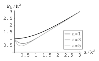
Figure 1: Modified propagator $P_{k}(z)=z+R_{k}(z)$; $a$ is a free parameter which determines the shape of $R_{k}$ (see Eq. (3)).

Effectively, these modes are suppressed in the functional integration, as required in Wilson’s formulation of the RG. The shape of $R_{k}$ is controlled by an arbitrary parameter $a$, which will be needed later on as a check of the consistency of the approximations. Explicitly, in momentum space:

$$R_{k}(z)=\frac{2a\,z\,e^{-2az/k^{2}}}{1-e^{-2az/k^{2}}}\quad\left(z=-\nabla^{2}\right).$$ (3)

Numerical values will always be given for $a=\frac{1}{2}$.

Eq. (2) can be generalized to gravity [6], adding gauge-fixing and ghost terms. Its r.h.s. becomes a sum over second derivatives w.r.t. all fields. Now the trace is over momenta and all quantum numbers, and $R_{k}$ is a matrix in the space of fields. Traces have been calculated using standard heat-kernel techniques in the regime $k^{2}\gg R$.

Eq. (2) boils down to an infinite number of ordinary first-order differential equations for the running couplings. To solve this system a convenient way is to adopt a truncation, namely one makes an ansatz such that $\Gamma_{k}$ is only made up of a suitable subset of all the admissible operators. One then rescales the dimensionful couplings with appropriate powers of $k$, ending up with the set of dimensionless couplings $\{g_{i}\}$. An FP is solution of the system $\beta_{i}=\partial_{t}g_{i}=0$, with $t=\log k$. To study its attractivity, one can use the linearized form of the flow equations,

$$\frac{\mathrm{d}g_{i}}{\mathrm{d}t}=M_{ij}\cdot g_{j}+\mathcal{O}\left(g^{2}\right),\quad M_{ij}=\left.\frac{\partial\beta_{i}}{\partial g_{j}}\right|_{FP},$$ (4)

since $\beta_{i}=0$ at the FP. We shall call $M$ the stability matrix. The solutions will be exponentials with the eigenvalues $\alpha_{i}$ of $M$ at the exponent, $\tilde{g}_{i}(t)\sim e^{\alpha_{i}t}$ (here $\tilde{g}_{i}$ is an eigenvector of $M$, a linear combination of the $g_{i}$’s). So the attractive directions for $k\to\infty$ will be those corresponding to eigenvalues of $M$ with a negative real part.

In the Einstein-Hilbert truncation, assuming $\Gamma_{k}=S_{E-H}$ with running $\Lambda$ and $\kappa$, one finds that there is a non-Gaussian FP (NGFP) which is attractive in both directions [7]. Introducing the dimensionless couplings $\hat{\Lambda}=k^{-2}\Lambda$ and $\hat{\kappa}=k^{-2}\kappa$, one finds that their values at the NGFP are $\hat{g}_{*}\equiv\left(16\pi\hat{\kappa}_{*}\right)^{-1}\!\!\approx 0.344$ and $\hat{\Lambda}_{*}\approx 0.339$. Here and in the following, the star denotes the values of the couplings at the FP. Therefore, at least in this approximation, the theory is asymptotically safe. The key point is to verify that the truncation does not bring about fake results. Many checks have been made; e. g., in an exact treatment one would expect independence of physical results from the cutoff function $R_{k}$, so the approximate solution should at most show a mild dependence, and this is indeed what happens [8, 9]. The major achievement, however, is that the addition of an $R^{2}$-term, thus considering a three-parameter truncation, does not change the results significantly, so the results obtained in the two-parameter Einstein-Hilbert truncation are trustworthy, and have a physical meaning. This was not a priori obvious: for instance, the GFP disappears, so this was really an artifact of the truncation.

3 Matter Fields

Now we extend the results found in [7] by including matter fields. To begin with, we have considered $\Gamma_{k}=S_{E-H}$ extended with $n_{S}$ real scalar, $n_{W}$ Weyl, $n_{M}$ Maxwell, and $n_{RS}$ (Majorana) Rarita-Schwinger fields, all massless and minimally coupled [10]. Then we have performed an analysis of the existence and attractivity of the NGFP varying the number of matter fields. Some results are shown in Fig. 2

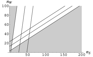
Figure 2: NGFP existence regions for $n_{RS}=0$. The gray area shows the existence region of the NGFP for $n_{M}=0$, delimited by the two most external lines, whereas the white zone is the non-existence region. Going away from the gray area, the straight lines represent the boundaries of the regions for $n_{M}=10$ and $n_{M}=20$, respectively. The existence region lies to the left and below these lines, being a translation of the gray area.

for $n_{RS}=0$. The existence regions are bounded by the lines of equations

$$n_{S}+2n_{M}-2n_{W}-4n_{RS}+6.16=0,$$ (5a)

$$6.6n_{S}-14n_{M}-1.6n_{W}+32n_{RS}-21=0.$$ (5b)

Eq. (5a) also discriminates between positive and negative cosmological constant. $\hat{\Lambda}_{*}$ is positive when the l.h.s. of Eq. (5a) is. Notice that it contains the difference between the total numbers of bosonic and fermionic degrees of freedom. In the existence region, the NGFP is always attractive in both directions.

Now one can apply the bounds given by Eqs. (5) to see whether the coexistence of gravity with a certain matter theory is still compatible with asymptotic safety. We have seen that popular GUT $SU(5)$ and $SO(10)$ theories indeed are, yielding a positive or negative $\hat{\Lambda}_{*}$ according to the symmetry-breaking pattern. The bounds we found are difficult to evade, since a large number of gauge bosons, as is the case for GUT theories, requires a large number of fermions, so one should introduce many fermion families to violate them. As for supersymmetric contents of matter, they all lie below the line of Eq. (5a), so in principle they would be compatible with asymptotic safety; however, we found that in this region numerical calculations are not reliable, depending quite strongly on the cutoff function, so in the present context we cannot say much about SUSY theories.

4 Gravity with a Scalar Field

Table 1: Stability matrix at the GMFP. The order of the variables is $\lambda_{0},\xi_{0},\lambda_{2},\xi_{2},\lambda_{4},\xi_{4},\dots$

$$\left(\begin{array}[]{ccccccccc}3.77&-7.64&-0.010&-0.013&0&0&0&0&\dots\\ 6.99&-7.94&0.0031&-0.019&0&0&0&0&\dots\\ 0&0&5.77&-7.64&-0.063&-0.078&0&0&\dots\\ 0&0&6.99&-5.94&0.019&-0.11&0&0&\dots\\ 0&0&0&0&7.77&-7.64&-0.16&-0.20&\dots\\ 0&0&0&0&6.99&-3.94&0.046&-0.28&\dots\\ 0&0&0&0&0&0&9.77&-7.64&\dots\\ 0&0&0&0&0&0&6.99&-1.94&\dots\\ \dots&\dots&\dots&\dots&\dots&\dots&\dots&\dots&\dots\end{array}\right)$$

An extension of the truncation considered in [10] would require a more detailed analysis of the matter couplings. It seems impossible to conceive calculations involving all admissible couplings present in a realistic matter theory, so as a first step we have considered the simplest example, that of a self-interacting scalar field [11]. Aside from its role as a model for the Higgs field in unified theories, a scalar field (the dilaton) appears in many popular theories of gravity. It can therefore sometimes be regarded as part of the gravitational sector, rather than the matter sector. This makes its properties especially interesting in a gravitational context.

The class of running actions that we have considered is

$$\Gamma_{k}[g,\phi]=\int\,\mathrm{d}^{4}x\sqrt{g}\;\cdot\\ \cdot\!\left(V(\phi^{2})-F(\phi^{2})R+{1\over 2}g^{\mu\nu}\partial_{\mu}\phi\partial_{\nu}\phi\right),$$ (6)

where the potential $V$ and the scalar-tensor coupling $F$ are arbitrary real analytic functions which can be expanded as a power series in $\phi^{2}$:

$$V(\phi^{2}) =\sum_{n=0}^{\infty}\tilde{\lambda}_{2n}\phi^{2n},$$ (7a)

$$F(\phi^{2}) =\sum_{n=0}^{\infty}\tilde{\xi}_{2n}\phi^{2n}.$$ (7b)

As before, we introduce dimensionless couplings $\lambda_{2n}=k^{2(n-2)}\tilde{\lambda}_{2n}$ and $\xi_{2n}=k^{2(n-1)}\tilde{\xi}_{2n}$. We shall take into account all of these couplings.

The theory admits an NGFP where all couplings vanish, apart from $\lambda_{0}=2\hat{\kappa}\hat{\Lambda}$ and $\xi_{0}=\hat{\kappa}$. Since all matter couplings vanish, we call it the “Gaussian-Matter” FP (GMFP). The values of the cosmological and Newton’s constant are only affected by the presence of the scalar kinetic term, and turn out to be $\hat{g}_{*}\approx 0.320$ and $\hat{\Lambda}_{*}\approx 0.359$ at the GMFP. The infinite-dimensional stability matrix is shown in Table 1. One can see that it has an almost block-diagonal form, and the diagonal blocks have a regular pattern. The eigenvalues reflect this regularity, being $-2.08\pm 4.38i$, $-0.08\pm 4.38i$, $1.92\pm 4.38i$,… . The real parts of the eigenvalues increase by constant multiples of two, so we can conclude that the critical surface has dimension four, and the theory is again asymptotically safe at the GMFP.

Therefore, we can see that even though matter is “Gaussian”, the gravitational interactions produce significant changes to the pure-scalar theory. For instance, the canonical dimension of the mass, which is $\frac{1}{2}\tilde{\lambda}_{2}$, changes from 2 to $\sim\!0.12$ (after mixing with $\xi_{2}$) and the usual quartic coupling, $\lambda_{4}$, becomes now an irrelevant parameter, its eigenvalue having a positive real part. The same pattern occurs for the other operators.

The analysis can be extended considering massless minimally coupled fields of different spins added to this gravity-scalar system. The outcome is that the NGFP is there, provided the matter content satisfies the bounds of Eqs. (5), and it is attractive in a possibly large number of directions. This could be a solution to the well-known problem of the triviality of the scalar theory; for a more detailed discussion of this issue see [11].

5 Parameter Dependence

As mentioned several times, a fundamental issue of this approach is to test whether the approximations assumed in the truncation are reliable. We can check whether physical results show a dependence on the cutoff function by looking at their dependence on the parameter a in Eq. (3).

To give an instance, we can consider the ratio $\lambda_{0*}/\xi_{0*}^{2}$, which is the inverse of the on-shell action, up to numerical factors. It is therefore an observable quantity, so in an exact treatment of our problem its value should be independent of $a$. The state of the art is depicted in Fig. (3).

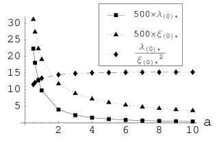
Figure 3: $\lambda_{0*}$, $\xi_{0*}$, and $\lambda_{0*}/\xi_{0*}^{2}$ as functions of $a$. The first two functions are magnified to get them in the same range of values as the last one.

It is remarkable that while $\lambda_{0*}$ and $\xi_{0*}$ display quite a substantial dependence on $a$, the ratio $\lambda_{0*}/\xi_{0*}^{2}$ is almost $a$-independent, giving an encouraging hint towards the reliability of the truncation. The stronger dependence of the latter quantity on $a$ for $a\to 0$ is due to the fact that in this limit $R_{k}$ becomes a constant, so it not trustworthy anymore as an IR cutoff.

Other cutoff-independent quantities are for instance the eigenvalues of $M$, which show a reasonably mild dependence on $a$ as well.

These results are in accordance with those of pure gravity [8, 9], from which they only differ slightly because of the presence of the scalar field.

6 Conclusions

In this talk we have presented the concept of asymptotic safety and reviewed the literature concerning its application to gravity theories in a nonperturbative context, with the use of ERGE. We have seen that the addition of massless, minimally coupled matter of different spins to the theory, which in principle might spoil these beautiful properties, can still yield an asymptotically safe theory, provided one satisfies some weak bounds on the matter content. The analysis of gravity coupled to a single scalar field with an arbitrary potential and coupling to the Ricci scalar, including infinitely many couplings, shows that the theory is asymptotically safe at a “Gaussian-Matter” FP. In this case the scalar sector allows for a perturbative treatment, whereas the gravity part is thoroughly non perturbative. The canonical dimensions of the pure-scalar theory are significantly changed by the gravitational corrections; this picture may ultimately yield a solution of the triviality issue in the scalar theory. The reliability of the approximations has also been checked, giving satisfying results. Therefore, this scenario has the potentiality of giving a consistent field theoretical description of gravity and matter.

References

- [1] S. Weinberg. In General Relativiy: An Einstein centenary survey, 790–831. Cambridge Univ. Press, 1979.
- [2] J. Polchinski. Nucl. Phys., B231:269–295, 1984.
- [3] C. Bagnuls and C. Bervillier. Phys. Rept., 348:91, 2001.
- [4] J. Berges, N. Tetradis, and C. Wetterich. Phys. Rept., 363:223–386, 2002.
- [5] C. Wetterich. Phys. Lett., B301:90–94, 1993.
- [6] M. Reuter. Phys. Rev., D57:971–985, 1998.
- [7] O. Lauscher and M. Reuter. Phys. Rev., D65:025013, 2002.
- [8] O. Lauscher and M. Reuter. Int. J. Mod. Phys., A17:993–1002, 2002.
- [9] O. Lauscher and M. Reuter. Class. Quant. Grav., 19:483–492, 2002.
- [10] R. Percacci and D. Perini. Phys. Rev., D67:081503, 2002.
- [11] R. Percacci and D. Perini. hep-th/0304222.