Transmission resonances and supercritical states in a one dimensional cusp potential

Abstract

We solve the two-component Dirac equation in the presence of a spatially one dimensional symmetric cusp potential. We compute the scattering and bound states solutions and we derive the conditions for transmission resonances as well as for supercriticality.

I Introduction

The study of scattering and bound states of nonrelativistic particles in the Schrödinger equation framework is a well known and understood problem Newton . The scattering of low momentum particles by one-dimensional potentials that are well behaved at infinity has zero transmission coefficient at zero energy, and the reflection coefficient is unity unless the potential supports a half bound state (zero energy resonance). In that case there is no reflection and the transmission coefficient is unity provided that the potential is symmetric. The pioneering works on the computation of transmission and reflection coefficients in one-dimensional potentials go back to Bohm Bohm who coined the definition of transmission resonance to scattering states with transmission coefficient equal to unity and vanishing reflection. Recently Senn ; Sassoli , these results have been generalized to asymmetric potentials.

The generalization of the concept of transition resonances to relativistic quantum mechanics presents some subtleties related to the Dirac equation Kennedy2 ; Dombey . For a free Dirac particle there are positive energy states $(E>m)$ as well as negative energy states $(E<-m)$. In the presence of an external potential, half bound states occur for $E=-m$ and $E=m$, in contrast to the non-relativistic case where these only exist at $E=0.$ In the Dirac equation framework one should talk about zero momentum resonances rather than zero energy resonances.

The study of scattering and bound states in the presence of strong electromagnetic fields in relativistic quantum mechanics is also a rather old problem. Soon after the formulation of the Dirac equation Dirac , Klein Klein found that for very high potential barriers an unusually large number of electrons penetrate into the wall. Moreover, those electrons have negative energy. Sauter Sauter found the same results in the more general case where the barrier smoothly grows. Pair creation for the Klein paradox is stimulated by the incoming electron beam. When the depth of a square well exceeds $2mc^{2}$, the energy of the lowest bound state becomes equal to $-mc^{2}$ , and the bound level joins the states of the Dirac sea. The bound states dive into the energy continuum Greiner .

The Klein paradox in a one-dimensional Saxon-Woods potential was studied by Dosch et al Dosch , showing that in this case transmission resonances exist. Kennedy Kennedy discussed supercriticality in this potential, demonstrating that, as in the square potential case, the one-dimensional Woods-Saxon potential has transmission resonances of zero momentum when it supports a half bound state at $E=-m$.

The Saxon-Woods potential presents the particularity of being a smoothed form of a square well; the Dirac equation presents half bound states with the same asymptotic behavior as those obtained with a potential barrier Kennedy .

In the present article we discuss the problem of computing transmission resonances and supercriticality of the one-dimensional symmetric screened potential (Fig 1):

$$U(x)=V_{0}\exp(-\left|x\right|/a).$$ (1)

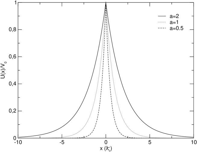
Figure 1: The screened potential for different values of the shape parameter $a(\lambdabar_{c})$. The solid line corresponds to $a=2$, the dotted line to $a=1$, and the dashed line to $a=0.5$

The potential (1) is an asymptotically vanishing potential for large values of the  space variable $x$. The parameter $V_{0}$ shows the height of the barrier or the depth of the well depending on its sign. The positive constant $a$ determines the shape of the potential. A noticeable difference between the Woods-Saxon potential and (1) is that this one does not exhibit a square barrier limit. The potential (1), for $V_{0}<0,$ can be regarded as a screened one dimensional Coulomb potential Dominguezadame .

It is the purpose of the present article to show that the potential (1), for $V_{0}>0$, supports transmission resonances. We solve the 1+1 Dirac equation explicitly and compute the bound energy states for $U(x),$ for $V_{0}<0,$ and show that this potential supports supercritical states which correspond to transmission resonances for the potential (1), for $V_{0}>0.$

The article is structured as follows. In Sec. II we solve the 1+1 Dirac equation in the potential (1). In Sec III we compute the bound states and the condition that the potential should satisfy in order to support supercritical states $(E=-m)$. In Sec. IV. we compute the scattering states and show that for $k=0$ the condition for transmission resonances corresponds to that of supercriticality for $V_{0}<0$.

II The Dirac equation

The Dirac equation in the presence of an external electromagnetic field $A_{\mu}$ has the form

$$\left\{\gamma^{\mu}(\partial_{\mu}-ieA_{\mu})+m\right\}\Psi=0,$$ (2)

where the four-vector potential (1) can be written in a covariant way as

$$A^{\mu}=V_{0}\exp(-\left|x\right|/a)\delta_{0}^{\mu}.$$ (3)

In two dimensions, the Dirac equation (2) in the presence of the spatially dependent electric field (3) reads

$$\left\{\gamma^{0}(\partial_{t}+ieV_{0}\exp(-\left|x\right|/a))+\gamma^{1}\partial_{x}+m\right\}\Psi=0$$ (4)

where the $\gamma^{\mu}$ matrices satisfy the commutation relation $\left\{\gamma^{\mu},\gamma^{\nu}\right\}=2\eta^{\mu\nu}$ and the metric $\eta^{\mu\nu}$ has the signature $(-,+).$ Here and throughout the present article we adopt units where $\hbar=c=1.$

Since we are working in 1+1 dimensions, it is possible to choose the following representation of the Dirac matrices

$$\gamma^{0}=i\sigma^{2}=\left(\begin{array}[]{cc}0&1\\ -1&0\end{array}\right),\ \gamma^{1}=\sigma^{1}=\left(\begin{array}[]{cc}0&1\\ 1&0\end{array}\right)$$ (5)

Taking into account that the vector potential (3) does not depend explicitly on time, we can separate the time dependence of the spinor $\Psi$ as follows:

$$\Psi=\left(\begin{array}[]{c}\Psi_{1}(x)\\ \Psi_{2}(x)\end{array}\right)\exp(-iEt)$$ (6)

Substituting the gamma matrices (5) into the Dirac equation, (4) we obtain the following system of coupled equations

$$\left(\frac{d}{dx}-i(eV_{0}\exp(-\left|x\right|/a)-E)\right)\Psi_{1}+m\Psi_{2}=0$$ (7)

$$\left(\frac{d}{dx}+i(eV_{0}\exp(-\left|x\right|/a)-E)\right)\Psi_{2}+m\Psi_{1}=0$$ (8)

Introducing the new variable

$$y=2iaeV_{0}\exp(-x/a)\ x\mathrm{>0}$$ (9)

we reduce the system (7)-(8) to

$$\left(y\frac{d}{dy}-\frac{y}{2}+iEa\right)\Psi_{2}=ma\Psi_{1}$$ (10)

$$\left(y\frac{d}{dy}+\frac{y}{2}-iEa\right)\Psi_{1}=ma\Psi_{2}$$ (11)

The regular solutions of the system of equations (10)-(11),can be expressed in terms of the Whittaker function $M_{k,\mu}(y)$  Abramowitz as follows

$$\Psi_{2}=b_{1}y^{-1/2}M_{k,\mu}(y)$$ (12)

$$\Psi_{1}=\frac{1/2+\mu+k}{ma}b_{1}y^{-1/2}M_{k+1,\mu}(y)$$ (13)

where $b_{1}$ is a normalization constant, and

$$k=iEa-1/2,\ \mu=i\sqrt{E^{2}-m^{2}}a$$ (14)

For negative values of $x$, we introduce the auxiliary variable $\bar{y}$

$$\bar{y}=2aieV_{0}\exp(x/a)\ x\mathrm{<0.}$$ (15)

In terms of the new variable $\bar{y},$ the system of equations (7)-(8) takes the form

$$\left(\bar{y}\frac{d}{d\bar{y}}+\frac{\bar{y}}{2}-iEa\right)\Psi_{2}+ma\Psi_{1}=0$$ (16)

$$\left(\bar{y}\frac{d}{d\bar{y}}-\frac{\bar{y}}{2}+iEa\right)\Psi_{1}+ma\Psi_{2}=0$$ (17)

and its solution can be written as

$$\Psi_{1}=c_{1}\bar{y}^{-1/2}M_{k,\mu}(\bar{y})$$ (18)

$$\Psi_{2}=-\frac{1/2+\mu+k}{ma}c_{1}\bar{y}^{-1/2}M_{k+1,\mu}(\bar{y})$$ (19)

where $c_{1}$ is a normalization constant

III Bound states

The potential (3) supports bound states provided that $m^{2}-E^{2}>0.$ In this case one has that $\mu$ can be written as

$$\mu=a\sqrt{m^{2}-E^{2}}$$ (20)

and the condition for existence of bound energy states can be obtained after imposing the normalizability of the wave function as well as the continuity of $\Psi$ at $x=0.$ Noticing the normalizability of the spinor $\Psi$ upon the scalar product

$$\left\langle\Psi,\Phi\right\rangle=\int\bar{\Psi}\gamma^{0}\Phi dx$$ (21)

imposes that the spinor components $\Psi_{1}$ and $\Psi_{2}$ should vanish as $\left|x\right|\rightarrow\infty$. This condition is equivalent to imposing the regularity of the spinor at $y=0,$ and $\bar{y}=0.$ The solutions (12)-(13), and (18)-(19) satisfy this boundary condition. The energy levels can be computed by imposing the continuity of the spinor $\Psi$ at $x=0.$

$$c_{1}M_{k,\mu}(2ieaV_{0})=b_{1}\frac{1/2+\mu+k}{ma}M_{k+1,\mu}(2ieaV_{0})$$ (22)

$$b_{1}M_{k,\mu}(2ieaV_{0})=-c_{1}\frac{1/2+\mu+k}{ma}M_{k+1,\mu}(2ieaV_{0})$$ (23)

The existence of non-trivial $c_{1}$ and $b_{1}$ satisfying the above system (22)-(23) is equivalent to imposing the condition

$$\left(\frac{1}{2}+\mu+k\right)^{2}M_{k+1,\mu}^{2}(2ieaV_{0})+m^{2}a^{2}M_{k,\mu}^{2}(2ieaV_{0})=0.$$ (24)

The expression (24) shows that the screened potential (1) is able to bind particles, a property that is absent in the purely one-dimensional Coulomb potential. The result (24) is equivalent to that obtained in Ref. Dominguezadame .

As the potential depth increases for large values of $V_{0}$, the energy eigenvalue of any bound state also decreases. When this energy reaches $E=-m$, the bound states merge with the negative energy continuum and the potential becomes supercritical. When $E=-m,$ $\mu=0$ and we obtain from Eq. (24) the condition for supercriticality:

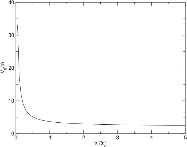
Figure 2: Dependence of the supercritical potential amplitude $V_{0}$ on the potential shape $a(\lambdabar_{c})$.

$$M_{k,0}(2ieaV_{0})M_{k,0}(2ieaV_{0})-M_{k+1,0}(2ieaV_{0})M_{k+1,0}(2ieaV_{0})=0$$ (25)

The condition (25) permits one to compute the value of $V_{0}$ for a given shape parameter $a$. Fig. 2. shows how depends the potential depth on the shape parameter $a.$

IV Scattering states

In order to discuss the transmission and reflection across the barrier given by the potential (3) , for $V_{0}>0,$we identify the incoming traveling wave. Since the vector potential (1) vanishes as $x\rightarrow-\infty$,  we have the result that the incoming wave should resemble a plane wave for large negative values of $x$. Looking at the asymptotic behavior of the Whittaker function $M_{k,\mu}(z)$ as $z\rightarrow 0$

$$M_{k,\mu}(z)\rightarrow\exp(-z/2)z^{\frac{1}{2}+\mu},$$ (26)

it is not difficult to obtain that the incoming wave reads

$$\Psi_{inc}(\bar{y})=\left(\begin{array}[]{c}\bar{y}^{-1/2}M_{k,\mu}(\bar{y})\\ -\frac{\frac{1}{2}+\mu+k}{ma}\bar{y}^{-1/2}M_{k+1,\mu}(\bar{y})\end{array}\right)$$ (27)

With the help of the relation (26), we obtain that, as $x\rightarrow-\infty,$ the spinor $\Psi_{inc}$ takes the form

$$\Psi_{inc}\rightarrow\left(\begin{array}[]{c}1\\ -\frac{\frac{1}{2}+\mu+k}{ma}\end{array}\right)(2ieaV_{0})^{\mu}\exp(ix\sqrt{E^{2}-m^{2}})$$ (28)

and consequently the spinor (27) satisfies the required asymptotic behavior. Analogously, we have that the reflected wave can be written as

$$\Psi_{refl}(\bar{y})=\left(\begin{array}[]{c}\bar{y}^{-1/2}M_{k,-\mu}(\bar{y})\\ -\frac{\frac{1}{2}-\mu+k}{ma}\bar{y}^{-1/2}M_{k+1,-\mu}(\bar{y})\end{array}\right)$$ (29)

as $x\rightarrow-\infty,$ we have that the reflected wave $\Psi_{refl}$ has the asymptotic  form

$$\Psi_{refl}\rightarrow\left(\begin{array}[]{c}1\\ -\frac{\frac{1}{2}-\mu+k}{ma}\end{array}\right)(2ieaV_{0})^{-\mu}\exp(-ix\sqrt{E^{2}-m^{2}})$$ (30)

The transmitted wave $\Psi_{trans}$ has the form

$$\Psi_{trans}(y)=\left(\begin{array}[]{c}\frac{\frac{1}{2}-\mu+k}{ma}y^{-1/2}M_{k+1,-\mu}(y)\\ y^{-1/2}M_{k,-\mu}(y)\end{array}\right)$$ (31)

whose asymptotic behavior for large values of $x$ is

$$\Psi_{trans}\rightarrow\left(\begin{array}[]{c}\frac{\frac{1}{2}-\mu+k}{ma}\\ 1\end{array}\right)(2ieaV_{0})^{\mu}\exp(ix\sqrt{E^{2}-m^{2}})$$ (32)

The computation of the reflection and transmission coefficients can be achieved with the help of the continuity of the spinor wave-function at the boundary $x=0$.

$$A\Psi_{inc}(x=0)+B\Psi_{refl}(x=0)=C\Psi_{trans}(x=0)$$ (33)

Substituting (27), (29) and  (31) into (33), we obtain

$$\frac{B}{A}=\frac{M_{k,\mu}(2ieaV_{0})M_{k,-\mu}(2ieaV_{0})-M_{k+1,\mu}(2ieaV_{0})M_{k+1,-\mu}(2ieaV_{0})}{-\frac{(\frac{1}{2}-\mu+k)^{2}}{m^{2}a^{2}}M_{k+1,-\mu}^{2}(2ieaV_{0})-M_{k,-\mu}^{2}(2ieaV_{0})}$$ (34)

The condition $B/A=0$ is equivalent to considering that there is no reflected wave, i.e, a transmission resonance condition. From Eq. (34) we obtain that a half bound state or zero momentum resonance condition $\mu=0$ satisfies the equation

$$M_{k,0}(2ieaV_{0})M_{k,0}(2ieaV_{0})-M_{k+1,0}(2ieaV_{0})M_{k+1,0}(2ieaV_{0})=0$$ (35)

Equation (35) gives the values of $V_{0}$  and $a$ for which zero momentum resonances exist. This condition, with $E=m,$ and $V_{0}>0,$ is equivalent to (25) for $E=-m$ and $V<0.$ In fact,  after taking the complex conjugate of Eq. (35),  using the the relation Gradshtein

$$z^{-\frac{1}{2}}M_{k,0}(z)=(-z)^{-\frac{1}{2}}M_{-k,0}(-z)$$ (36)

for the Whittaker functions, and substituting the value of $k$ defined by the relation (14), we reobtain the supercriticality condition (25). The dependence of $V_{0}$ on $a$ for transmission resonance states is shown in Fig. 2.

V Concluding remarks

The relations (25) and (35) show that the one dimensional screened potential (1) supports supercritical states and consequently half bound states. This result is not trivial in view of the fact that the one-dimensional Coulomb potential presents only scattering states Dominguez2 . The potential (1) does not exhibit a square barrier limit, and for very small values of $a$ and constant value of $V_{0}a$ it can be regarded as a delta potential Dominguezadame ; therefore the relations (25) and (35) also hold for a delta potential. The results obtained in this paper show that very cusp symmetric potentials also support half bound states.

.

- (1) R. G. Newton Scattering Theory of Waves and Particles (Springer, Berlin, 1982)
- (2) D. Bohm Quantum Mechanics (Prentice-Hall New York, 1951)
- (3) P. Senn, Am. J. Phys. 56, 916 (1988).
- (4) M. Sassoli de Bianchi, J. Math. Phys. 35, 2719 (1994).
- (5) P. Kennedy and N. Dombey, J. Phys. A 35, 6645 (2002)
- (6) N. Dombey, P. Kennedy, and A. Calogeracos Phys. Rev. Lett. 85 1787 (2000).
- (7) P. A. M. Dirac, Proc. R. Soc. A 117, 610 (1928).
- (8) O. Klein, Z. Phys. 53, 157 (1929).
- (9) N. Sauter, Z. Phys. 69, 742 (1931).
- (10) W. Greiner, B. Müller, and J. Rafelski Quantum Electrodynamics of Strong Fields (Springer: Berlin, 1985)
- (11) H. G. Dosch, J. H. D. Jensen, and V. F. Müller, Phys. Norvegica 5, 151 (1971).
- (12) P. Kennedy, J. Phys. A 35, 689 (2002).
- (13) M. Abramowitz, and I. A. Stegun, Handbook of Mathematical Functions (New York: Dover, 1965).
- (14) F. Domínguez-Adame, and A. Rodríguez, Phys. Lett. A. 198, 275 (1995).
- (15) I. S. Gradshtein, and I. W. Ryzhik, Table of Integrals, Series and Products (Academic, New York, 1984).
- (16) F. Domínguez-Adame, and E. Maciá, Europhys. Lett. 8, 711 (1989).