hep-th/0305024
Localized anomalies in orbifold gauge theories 

Abstract

We apply the path-integral formalism to compute the anomalies in general orbifold gauge theories (including possible non-trivial Scherk-Schwarz boundary conditions) where a gauge group $\mathcal{G}$ is broken down to subgroups $\mathcal{H}_{f}$ at the fixed points $y=y_{f}$. Bulk and localized anomalies, proportional to $\delta(y-y_{f})$, do generically appear from matter propagating in the bulk. The anomaly zero-mode that survives in the four-dimensional effective theory should be canceled by localized fermions (except possibly for mixed $U(1)$ anomalies). We examine in detail the possibility of canceling localized anomalies by the Green-Schwarz mechanism involving two- and four-forms in the bulk. The four-form can only cancel anomalies which do not survive in the 4D effective theory: they are called globally vanishing anomalies. The two-form may cancel a specific class of mixed $U(1)$ anomalies. Only if these anomalies are present in the 4D theory this mechanism spontaneously breaks the $U(1)$ symmetry. The examples of five and six-dimensional $\mathbb{Z}_{N}$ orbifolds are considered in great detail. In five dimensions the Green-Schwarz four-form has no physical degrees of freedom and is equivalent to canceling anomalies by a Chern-Simons term. In all other cases, the Green-Schwarz forms have some physical degrees of freedom and leave some non-renormalizable interactions in the low energy effective theory. In general, localized anomaly cancellation imposes strong constraints on model building.

April 2003

1 Introduction

The existence of extra dimensions (on top of the four space-time coordinates) is a general feature of theories aiming to unify all known interactions (including gravity) with quantum mechanics. In particular string theories predict six, and M-theory seven, extra dimensions and it is widely believed that all string theories are related to each other by various string dualities [1]. Unlike in the case of the perturbative heterotic string where all scales –the string ($M_{s}$) and the compactification ($M_{c}$) scales– are close to each other and to the four-dimensional Planck scale, in some recent string constructions (as e. g. non-perturbative heterotic string or type I strings) it has been shown that both the string length [2] and (some of the) compactification radii can lie in the range of the inverse TeV length, with possible interesting phenomenological implications [3]. Moreover the existence of branes (e. g. D-branes in type I strings [1]) makes it possible that the Standard Model fields propagate in a brane with $p$ longitudinal dimensions spanning a $(4+p)$-dimensional ($p\geq 1$) world-sheet while gravity propagates in the bulk of the higher-dimensional space where the transverse dimensions can be as large as the submillimeter size, thus “explaining” the smallness of four-dimensional gravitational interactions [4]. In that case, if there is a little hierarchy between the string and compactification scales ($M_{s}/M_{c}\gg 1$) the Standard Model interactions are described by an effective field theory in $(4+p)$-dimensions with a cutoff at $\Lambda\simeq M_{s}$ [5]. This opened up the exciting possibility of new physics beyond the Standard Model scale and below the string scale with large (TeV) extra dimensions and towers of Kaluza-Klein states that can give rise to new phenomenology at future colliders [6] and to new mechanisms for old phenomena as supersymmetry and electroweak symmetry breaking [7]. In particular non-trivial compactification of the extra dimensions, as orbifold compactification [8] and Scherk-Schwarz boundary conditions [9], can shed some light on those problems.

The previous ideas gave rise to a plethora of field-theoretical models in extra dimensions [10, 11] where both phenomenological and theoretical studies have recently been developed. However, unlike in string constructions where the consistency of the theory is guaranteed by the symmetries of the string (e. g. modular invariance in heterotic string models) in field-theoretical ones this consistency must be imposed. In particular one of the main ingredients coming automatically in string models, i e. anomaly freedom, must be enforced in field-theoretical models. This requisite is a very important one since it is responsible for the consistency of the theory at the quantum level. Moreover since anomalies are an infra-red phenomenon their cancellation is a common requirement where both string and field theory constructions should meet. Put differently, since anomalies are generated by the massless spectrum they are a common feature of any string theory and any effective field theory descending from it. To conclude, anomaly cancellation in field theories in extra dimensions is a requirement for the consistency of the corresponding theory at the quantum level and also a requirement for it to descend from an underlying string theory.

The question of anomaly cancellation in field-theoretical models in the presence of extra dimensions has recently been addressed. The first step in this direction was given in Ref. [12] where a simple five-dimensional model compactified on the orbifold $S^{1}/\mathbb{Z}_{2}$ was considered. It was observed that the five-dimensional anomaly was localized at the orbifold fixed points $y=0,\pi R$ while there was no bulk anomaly, a simple consequence of the fact that the five-dimensional theory is non-chiral. However cancellation of localized anomalies was automatically induced by cancellation of anomalies in the four-dimensional theory. This feature was proven not to be a general one in subsequent studies of the orbifold $S^{1}/\mathbb{Z}_{2}\otimes\mathbb{Z}^{\prime}_{2}$ [13, 14, 15, 16, 17, 18] where cancellation of anomalies in the four-dimensional theory did not imply cancellation of localized anomalies. However it was proven that the latter could be achieved by the introduction of a Chern-Simons counterterm without affecting the four-dimensional effective theory. The anomalies in particular higher-dimensional (string and field-theoretical) models have been very recently under consideration [19, 20, 21, 22, 23].

The aim of this paper is to see how localized anomalies can be computed in arbitrary orbifold models in any dimension and how the cancellation by the Green-Schwarz mechanism generalizes to those cases. We consider orbifolds defined on an arbitrary $(D-4)$-dimensional compact space $C$ modded out by an arbitrary discrete group $\mathbb{G}$ acting non-freely on $C$ with fixed points at $y=y_{f}$. Our purpose is to obtain general features of localized anomalies and anomaly cancellation that could be held by any orbifold construction. We assume an arbitrary gauge group in the bulk $\mathcal{G}$ broken by the orbifold action to subgroups $\mathcal{H}_{f}$ at the fixed points and with possible Scherk-Schwarz boundary conditions. We have proved that, as expected, the absence of anomalies in the four-dimensional theory of zero modes can not cope with the cancellation of localized anomalies in arbitrary orbifolds. We then study the contribution to anomalies from Green-Schwarz (GS) $p$-forms propagating in the bulk [24]. It turns out that in general two and four-forms (or their corresponding duals) can contribute to localized anomalies and eventually cancel existing ones . We will define globally vanishing localized anomalies those whose zero-modes vanish upon integration over the extra dimensions and thus do not survive in the four-dimensional effective theory. The localized anomalies whose zero-modes survive in the four-dimensional theory are consequently called globally non-vanishing anomalies.

The contribution from the two-form is always a mixed $U(1)$ anomaly, which can be globally vanishing or not. In case it is globally non-vanishing, the $U(1)$ will be spontaneously broken in the low energy theory. In the four-dimensional (4D) limit we are left with non-renormalizable interactions which depend on the compactification. In 5D models we find an axion $a(x)$, coupling at low energy like

$$a\,\text{tr}\,F_{[\mu\nu}F_{\rho\sigma]}\epsilon^{\mu\nu\rho\sigma},$$ (1.1)

while in $6D$ compactifications we find in addition zero mode-interactions of two-forms as

$$C_{\mu\nu}\text{tr}\,F_{[\rho\sigma}F_{56]}\epsilon^{\mu\nu\rho\sigma}.$$ (1.2)

The contribution from the GS four-form gives all kind of pure gauge anomalies, but no mixed $U(1)$ gravitational ones if $\mathcal{G}$ is simple. Those anomalies are always globally vanishing, which is consistent with the fact that non-abelian anomalies can not be canceled by GS in 4D. As a consequence, GS cancellation of this kind of anomalies can only work for anomalies which do not have any zero mode, i.e. are globally vanishing. In the 5D models, a four-form has no physical degrees of freedom and can thus be integrated out algebraically, leaving over precisely the CS counterterm found earlier in the literature. In 6D, the four-form has an axionic degree of freedom which in general compactifications will have a zero mode $a(x)$, leaving the following non-renormalizable coupling at low energy:

$$a\,\text{tr}\,F_{[\mu\nu}F_{\rho\sigma}F_{56]}\epsilon^{\mu\nu\rho\sigma},$$ (1.3)

In both cases we will find that the localized anomalies generated by the GS forms have a quite peculiar form, which considerably restricts the possibility of canceling the localized anomalies produced by bulk and brane fermions.

The outline of this paper is as follows. In section 2 the different projectors that appear in the orbifold construction are defined and the gauge structure localized at the different fixed points described. Section 3 is devoted to the introduction of Scherk-Schwarz non-trivial boundary conditions in the orbifold structure. The equivalence between Scherk-Schwarz [9] and Hosotani [26] breaking is not guaranteed (especially in orbifolds in $D\geq 6$ dimensions) and the conditions for it are explicitly established. An important case where this equivalence does not hold is when the Scherk-Schwarz breaking proceeds through discrete Wilson lines along the Cartan subalgebra, in which case the corresponding orbifold can be described by a different one with periodic fields defined on a larger torus modded out by a larger discrete group. While the Hosotani mechanism spontaneously breaks the gauge group in the zero mode sector but not the gauge groups localized on the branes, the latter breaking is possible in the SS-mechanism and naturally has an impact on the anomalies localized at the fixed points. In section 4 the path-integral method [27] is applied to compute the anomalies in the previously defined orbifold structure. A bulk term, corresponding to anomalies in the higher-dimensional gauge theory, and localized terms on the orbifold fixed points are obtained. The structure of the localized anomalies is disentangled in general. In section 5 the cancellation of localized anomalies by the Green-Schwarz mechanism is studied. The Green-Schwarz $p$-forms in the bulk in general lead to bosonic degrees of freedom in the 4D effective theory with non-renormalizable interactions that could have some phenomenological consequences. $\mathbb{Z}_{N}$ orbifolds in $D=5$ and $D=6$ are analyzed in great detail in section 6 whose results could be easily applied to different orbifold and gauge constructions. Finally section 7 contains our conclusions and appendices A and B some useful conventions and technical details about the orbifolds studied in section 6.

2 Orbifold projectors

In this section we will consider a generic orbifold defined in $D-4$ extra dimensions and the corresponding projectors that will be used in the calculation of the brane anomalies section 4. The starting point is the $C/\mathbb{G}$-orbifold $M^{4}\times C/\mathbb{G}$, where $C$ is a compact $(D-4)$-dimensional manifold (e.g. a torus $T^{D-4}$) which is modded out by the discrete group $\mathbb{G}$ that acts non-freely on $C$. We will parametrize $M^{4}\times C$ with the coordinates $x^{M}$ which we split into $(x^{\mu},x^{i}\equiv y^{i})$, $\mu=0,\dots,3$ and $i=1,\dots,D-4$. The orbifold is constructed by identifying the orbits of $\mathbb{G}$, i.e.

$$x\sim P_{k}x$$ (2.1)

where the operators $P_{k}$ acting on $C$ are a representation of the group elements $k\in\mathbb{G}$. Since $\mathbb{G}$ is acting non-freely on $C$ it means that given $k\in\mathbb{G}$ there are some points $y_{kf}\in C$ such that $P_{k}y_{kf}=y_{kf}$. The set $\{y_{kf}\}$ are the fixed points of the $k$-sector of the orbifold. For some orbifolds the set $\{y_{f}\}\equiv\cup_{k}\{y_{kf}\}$ constitutes a hypersurface inside $C$ in which case they are correspondingly called fixed lines, planes, etc. We will call generically these sets as fixed points.

The orbifold group $\mathbb{G}$ also has a representation on the fields:

$$\phi(x)\rightarrow\lambda_{k}\otimes{\cal P}_{k\,\sigma}~{}\phi(P_{k}^{-1}x)$$ (2.2)

where ${\cal P}_{k\,\sigma}$ acts on the fermionic indices of the field $\phi$, determined by the spin $\sigma$, and $\lambda_{k}$ acts on internal gauge and flavor indices. We assume that the theory in the bulk of the extra dimensions is a D-dimensional gauge theory with gauge group $\mathcal{G}$ and the field $\phi$ transforms as an (irreducible) representation $R$ of $\mathcal{G}$. The matrices ${\cal P}_{k\,\sigma}$ and $\lambda_{k}$ must form representations of $\mathbb{G}$. According to the identification of Eq. (2.1) we then have 

$$\phi(x)=\lambda_{k}\otimes{\cal P}_{k\,\sigma}~{}\phi(P_{k}^{-1}x),\qquad\forall k\in{\mathbb{G}}$$ (2.3)

These are the $N\equiv|G|$ orbifold constraints the fields have to satisfy.

We now introduce the action of $\mathbb{G}$ on function space by defining the unitary operator

$$\hat{P}_{k}|x\rangle=|P_{k}x\rangle,\qquad\langle x|\hat{P}_{k}=\langle P_{k}^{-1}x|.$$ (2.4)

Eq. (2.3) can then be rewritten as a linear operation on the space of fields on the torus, $|\phi\rangle$ (where $\phi(x)\equiv\langle x|\phi\rangle$), as

$$(1-\lambda_{k}\otimes{\cal P}_{k\,\sigma}\otimes\hat{P}_{k})|\phi\rangle=0,\qquad\forall k\in{\mathbb{G}}.$$ (2.5)

We are looking for a projector $Q_{\phi}$ which, acting on a generic field $\phi$ on $C$ gives a field which satisfies Eq. (2.5). In other words $Q_{\phi}$ should satisfy the conditions

$$(1-\lambda_{k}\otimes{\cal P}_{k\,\sigma}\otimes\hat{P}_{k})Q_{\phi}=0,\qquad\forall k\in{\mathbb{G}}.$$ (2.6)

One can easily check that $Q_{\phi}$ is given by

$$Q_{\phi}=\frac{1}{N}\sum_{k}\lambda_{k}\otimes{\cal P}_{k\,\sigma}\otimes\hat{P}_{k},$$ (2.7)

where the factor $1/N$ guarantees that $Q^{2}_{\phi}=Q_{\phi}$ and we also have $Q_{\phi}^{\dagger}=Q_{\phi}$. Note that the sum includes also the unit element. A further property of $Q_{\phi}$ is that it is gauge invariant $g^{-1}Q_{\phi}g=Q_{\phi}$ since it commutes with $\xi(x)\equiv\xi^{A}(x)T^{A}$, $g=\exp\{i\xi(x)\}$. For later use we also note that given a projection $Q_{\psi}$ for a fermion $\psi$, such that $Q_{\psi}\psi$ defines a constrained spinor, the projector for the Dirac conjugate $Q_{\bar{\psi}}$ is related to it as

$$Q_{\bar{\psi}}=\Gamma^{0}Q_{\psi}\Gamma^{0},$$ (2.8)

and $\bar{\psi}Q_{\bar{\psi}}$ defines the corresponding constrained spinor on the orbifold.

In general, the orbifold action of $k\in\mathbb{G}$ can break the gauge group $\mathcal{G}=\{T^{A}\}$ in the bulk to a subgroup $\mathcal{H}_{f}$ at the fixed point $y_{f}$. We assign a ${\mathbb{G}}$ transformation to the generators according to

$$T^{A}\rightarrow\Lambda_{k}^{AB}T^{B},$$ (2.9)

which must be an automorphism on the algebra, i.e. leave the structure constants invariant. Whenever we can write this transformation as a group conjugation, i.e. $\Lambda_{k}^{AB}T^{B}=g_{k}T^{A}g_{k}^{-1}$, this is called an inner automorphism. It takes a simple structure in terms of the Weyl-Cartan basis $\{T^{A}\}=\{E_{\alpha},H_{j}\}$ where we can always choose $g_{k}$ to be of the form $g_{k}=\exp(-2\pi i\vec{V}_{k}\cdot\vec{H})$ where $\vec{V}_{k}$ is the rank($\mathcal{G}$)-dimensional twist-vector that defines the orbifold breaking. We then simply have $\Lambda^{ij}=\delta^{ij}$, $\Lambda_{k}^{i\alpha}=0$ and $\Lambda^{\alpha\beta}=\exp\{-2\pi i\,\vec{\alpha}\cdot\vec{V}_{k}\}\,\delta^{\alpha\beta}$ where $\vec{\alpha}$ is the rank($\mathcal{G}$)-dimensional root associated to the generator $E_{\alpha}$. If Eq. (2.9) cannot be written as a group conjugation it is called an outer automorphism. An important example is the ${\mathbb{Z}}_{2}$ outer automorphism which takes $T_{A}\rightarrow-T_{A}^{T}$.

After choosing the breaking pattern $\Lambda_{k}$, the gauge bosons satisfy Eq. (2.3) with $\lambda_{k}=\Lambda_{k}$ and ${\mathcal{P}}_{k,\,1}=P_{k}$. At each fixed point $y_{f}$, the elements $k\in\mathbb{G}$ which leave $y_{f}$ fixed form a subgroup $\mathbb{G}_{f}\subset\mathbb{G}$. By diagonalizing $\Lambda$, the unbroken gauge group at each fixed point is $\mathcal{H}_{f}=\{T^{A}~{}|~{}\Lambda_{k}^{AA}=1\ \forall k\in\mathbb{G}_{f}\}$ since only gauge bosons $A_{\mu}^{A}$ corresponding to these generators are non-vanishing at $y_{f}$. Furthermore, the unbroken gauge group in the effective four-dimensional theory is given by $\mathcal{H}=\{T^{A}~{}|~{}\Lambda_{k}^{AA}=1\ \forall k\in\mathbb{G}\}$ since this defines the set of massless 4D gauge bosons. We will simply write $\mathcal{H}=\{T^{a}\}$ and $\mathcal{G/H}=\{T^{\hat{a}}\}$. Clearly, ${\mathcal{H}}=\cap_{f}{\mathcal{H}}_{f}$, so in particular ${\mathcal{H}}$ is a subgroup of all ${\mathcal{H}}_{f}$. We will denote the generators of $\mathcal{H}_{f}=\{T^{a_{f}}\}$ and $\mathcal{G}/\mathcal{H}_{f}=\{T^{\hat{a}_{f}}\}$, where the set $\{T^{\hat{a}_{f}}\}$ is a subset of $\{T^{\hat{a}}\}$. In particular for fixed points such that $\mathbb{G}_{f}=\mathbb{G}$, one gets $\mathcal{H}_{f}=\mathcal{H}$.

If there are matter fields transforming in some representation of $\mathcal{G}$, we must have

$$\lambda_{k}T^{A}\lambda^{-1}_{k}=\Lambda_{k}^{AB}T^{B}.$$ (2.10)

in order to get invariance of the action under $\mathbb{G}$. Note that if the automorphism Eq. (2.9) is an inner one, this condition is satisfied by just identifying $\lambda_{k}$ with $g_{k}$ evaluated in the appropriate representation. If the automorphism is an outer one, there might be restrictions on the representations in order to find such a $\lambda_{k}$. Note that the projectors $\lambda_{k}$ have to satisfy the commutation property with the unbroken generators $T^{a_{f}}$,

$$[\lambda_{k},T^{a_{f}}]=0.$$ (2.11)

3 Scherk-Schwarz versus Hosotani breaking

In this section we will consider the case of general orbifolds in the presence of Scherk-Schwarz [9] boundary conditions and their relation to the Hosotani [26] mechanism. We will analyze the conditions under which those two breakings are equivalent and find the cases where they are not, with the subsequent impact on the possible localized anomalies in particular models.

In theories with non-simply connected internal dimensions, as orbifolds, fields may possess non-trivial boundary conditions when moving along a closed but non-contractible cycle. Invariance of the action is guaranteed as long as the resulting multiple values of the field are related by an internal (local or global) symmetry transformation (twist):

$$\phi(y^{i}+2\pi n^{i})=W(n^{i})\phi(y^{i}),\qquad W(n^{i})=\exp(2\pi in^{i}\Omega_{i}).$$ (3.1)

The boundary conditions defined in Eq. (3.1) are known as Scherk-Schwarz (SS) boundary conditions [9]. Here $\vec{n}$ is a lattice vector, $W(\vec{n})$ is the Wilson line along the direction $\vec{n}$ and $\Omega_{i}=\omega_{i}^{A}T^{A}$ where $T^{A}$ are the generators of the internal symmetry and $\omega_{i}^{A}$ the SS-parameters. To make sense out of the boundary condition (3.1) one has to demand that Wilson lines along different directions commute , i. e.

$$[W(n^{i}),W(m^{i})]=0\,\Longleftrightarrow\,[\Omega_{i},\Omega_{j}]=0\ .$$ (3.2)

The corresponding symmetry is then broken in the presence of the Wilson lines $W(\vec{n})$. Notice that condition (3.2) is trivially satisfied for the case of one extra dimension ($D=5$). For higher-dimensional theories ($D\geq 6$) it imposes a non-trivial restriction on the SS-breaking patterns.

In the case of a local symmetry, one can sometimes undo this twist by means of a non-periodic gauge transformation which only depends on the extra coordinates, $g(y)$. All fields become then periodic but some extra components of the gauge fields acquire a vacuum expectation value (VEV). This is known as the Hosotani-mechanism [26]. The obvious guess to achieve periodic fields is the gauge transformation $g(y)=\exp(-iy^{i}\Omega_{i})$ and one immediately obtains $\langle A_{i}\rangle=\Omega_{i}$. However, a constant VEV for $A_{i}$ is only possible if this configuration is left invariant by the orbifold action, thus obtaining the constraint 

$$\langle A_{i}\rangle=P_{i}^{j}\lambda_{k}\langle A_{j}\rangle\lambda_{k}^{-1}.$$ (3.3)

where $P_{i}^{j}$ is a matrix representation acting over the space indices of the orbifold element $P_{k}$. Obviously only SS–breaking satisfying the parallel constraint

$$\Omega_{i}=P_{i}^{j}\lambda_{k}\Omega_{j}\lambda_{k}^{-1}.$$ (3.4)

can be given a Hosotani interpretation. Note that the latter one is the same constraint $\Omega_{i}$ has to satisfy if the gauge transformation is to be consistent with the orbifold, i. e.  if condition

$$g(P_{k}y)=\lambda_{k}g(y)\lambda_{k}^{-1}.$$ (3.5)

holds. This equation is precisely fulfilled by $g(y)=\exp(-iy^{i}\Omega_{i})$ if $\Omega_{i}$ satisfies Eq. (3.4). For the case of one extra dimension the $\mathbb{Z}_{2}$ orbifold action is $P^{5}_{5}=-1$ and condition (3.4) on $\Omega\equiv\Omega_{5}$ gives $\{\Omega,\lambda\}=0$, or equivalently $W\lambda W=\lambda$ which provides the usual consistensy condition on possible twist operators $\lambda$ in the $S^{1}/\mathbb{Z}_{2}$ orbifold [10].

On the other hand, starting from the Hosotani mechanism in the presence of a constant background $\langle A_{i}\rangle$ sometimes one can also transform periodic fields into fields satisfying the Scherk–Schwarz boundary conditions. In fact a constant VEV can only be gauged away provided that

$$F_{ij}=[A_{i},A_{j}]=0$$ (3.6)

in agreement with the condition (3.2). Notice that again [as it happened with the consistency of the SS-boundary conditions in (3.2)] for the case of one extra dimension the condition (3.6) is trivially satisfied, which shows that for the $D=5$ case the Hosotani breaking can always be intepreted as a Scherk-Schwarz [28] breaking . Again for higher-dimensional theories ($D\geq 6$) the condition (3.6) is non-trivial. We summarize the relation between the SS and Hosotani mechanisms in Fig. 1.

$$\left\{\begin{array}[]{c}\framebox{\text{Hosotani}}\\ \\ \phi(y^{i}+2\pi n^{i})=\phi(y^{i})\\ \langle A_{i}\rangle=const\\ \langle A_{i}\rangle=P_{i}^{j}\lambda_{k}\langle A_{j}\rangle\lambda_{k}^{-1}\end{array}\right\}\begin{array}[]{c}\xrightarrow{\hskip 11.38092pt{[A_{i},A_{j}]=0}\hskip 11.38092pt}\\ \xleftarrow[\Omega_{i}=P_{i}^{j}\lambda_{k}\Omega_{j}\lambda_{k}^{-1}]{}\end{array}\left\{\begin{array}[]{c}\framebox{\text{Scherk--Schwarz (Wilson--Line)}}\\ \\ \phi(y^{i}+2\pi n^{i})=\exp(2\pi in^{i}\Omega_{i})\phi(y^{i})\\ \langle A_{i}\rangle=0\\ \left[\Omega_{i},\Omega_{j}\right]=0\end{array}\right\}$$ (3.7)

Figure 1: The relation between SS and Hosotani breaking. The two schemes are equivalent if the respective constraints specified in the lowest row can be satisfied simultaneously. In this case there exists a non-periodic gauge transformation which gives $\Omega_{i}=\langle A_{i}\rangle$.

The Scherk-Schwarz boundary conditions change the periodicity of the fields and thus in principle the surviving gauge groups ${\mathcal{H}}_{f}$ in the branes, which in turn determines the possible localized matter content. To determine the unbroken gauge group at a given fixed point $y_{f}$ in the presence of SS-twists, one has to identify the gauge fields whose boundary conditions do not force them to vanish at $y_{f}$. Since fields are in general non-periodic, we have to work on the covering space of the torus where the boundary conditions applied at the fixed point $y_{f}$ give

$$A_{\mu}(P_{k}y_{f})\equiv A_{\mu}(y_{f}+2\pi n_{f,k})=W(n_{f,k})A_{\mu}(y_{f})W^{-1}(n_{f,k})=\lambda_{k}A_{\mu}(y_{f})\lambda_{k}^{-1}$$ (3.8)

Here $k$ is restricted to the orbifold subgroup ${\mathbb{G}}_{f}$ defined at the end of the previous section. The second equality reflects the SS boundary condition, while the last one the orbifold boundary condition. The unbroken subgroup ${\mathcal{H}}_{f}^{W}$ is thus spanned by the generators that commute with $W^{-1}(n_{f,k})\lambda_{k}$. Since, in the absence of SS–boundary conditions, the unbroken subgroup at the fixed point $y_{f}$ ($\mathcal{H}_{f}$) was defined as the subgroup commuting with $\lambda_{k}$, $k\in\mathbb{G}_{f}$, it is clear that generically ${\mathcal{H}}_{f}^{W}$ will be different from $\mathcal{H}_{f}$. However if the SS-breaking can be given a Hosotani interpretation we will see that they coincide, i. e. ${\mathcal{H}}_{f}^{W}=\mathcal{H}_{f}$. In fact using Eq. (3.5) one can easily check that $W^{-1}(n_{f,k})\lambda_{k}=g^{-1}(y_{f})\lambda_{k}g(y_{f})$, where $g(y)=\exp(-iy^{i}\Omega_{i})$ is the gauge transformation which relates the SS and Hosotani pictures. Consequently, when switching on the SS twist, the brane gauge group ${\mathcal{H}}_{f}^{W}$ becomes $g^{-1}(y_{f}){\mathcal{H}}_{f}g(y_{f})$ and thus is equivalent to the one without SS-breaking. At the end this is expected, since in the Hosotani picture all fields remain periodic and so ${\mathcal{H}}_{f}$ is unaffected by the VEV $\langle A_{i}\rangle$.

However, the brane gauge group can change when there is a Scherk-Schwarz breaking that can not be given a Hosotani interpretation. This case is most commonly referred to as “discrete Wilson line” breaking. A trivial way to satisfy the consistency condition (3.2) it to choose the Wilson line generators to lie in the Cartan subalgebra,

$$\Omega_{i}=\omega_{i}^{I}H_{I}.$$ (3.9)

Let us look at the example of a torus modded out by the cyclic group $\mathbb{G=Z}_{N}$. The action on the extra coordinates $y$ is given by $P^{n}$, $0\leq n<N$ with $P^{N}=1$, where $P_{i}^{j}$ does not contain unit eigenvalues. Then in order to have a Hosotani interpretation [Eq. (3.4)] one would have to satisfy the equation $P_{i}^{j}\Omega_{j}=\Omega_{i}$, a condition that can not be fulfilled since $\det(P-1)\neq 0$ . Using the fact that $\sum_{n}P^{n}=0$, the purely geometrical identity

$$(\tau(n^{i})P)^{N}=1,\qquad\tau(n^{i}):y^{i}\rightarrow y^{i}+2\pi n^{i}.$$ (3.10)

is satisfied. This identity is reflected on the fields and one thus obtains $(W(n^{i})\lambda)^{N}=W^{N}\lambda^{N}=W^{N}=1$ which implies that $N\omega_{i}^{I}=\text{integer}$ and the Wilson lines turn out to be discrete. As a concrete example consider $S^{1}/{\mathbb{Z}}_{2}$ with ${\mathcal{G}}=SU(3)$ broken down to ${\cal H}={\cal H}_{0}={\cal H}_{\pi}=SU(2)\otimes U(1)$ by the inner automorphism characterized by the twist vector $V=({\frac{1}{2}},0^{7})$ or equivalently $\lambda=\text{diag}(-1,-1,1)$. Taking $\omega_{5}^{I}=V^{I}$ the new gauge group ${\cal H}_{\pi}$ is $SU(3)$, since $W^{-1}(-1)\lambda=1$ now commutes with all generators.

In most cases it will be possible to find an equivalent description in terms of a different orbifold without Wilson lines. In particular, the relation $W^{N}=1$ implies that on the bigger torus $T^{\prime p}$ with radius $R^{\prime}=NR$ there are no Wilson lines. One obtains the same physical space (and the same physical theory) by modding out $T^{\prime p}$ with the bigger orbifold group $\mathbb{G}^{\prime}$ generated by $\{P,\tau(\hat{n}_{i})\}$, where $\hat{n}_{i}$ are the basis vectors defining the lattice of $T^{p}$. In the above example this amounts to the orbifold group $\mathbb{Z}_{2}\otimes\mathbb{Z}_{2}^{\prime}$ [11] defined on the circle with twice the radius.

4 Anomalies in orbifolds

In this section we will apply the path-integral method of anomaly evaluation [27] to compute the anomalies in orbifold gauge theories. In chiral gauge theories anomalies arise if the measure in the functional integral is not invariant under gauge symmetry transformations $\xi(x)$:

$${\cal D}\psi{\cal D}\bar{\psi}\rightarrow{\cal D}\psi{\cal D}\bar{\psi}\exp(i{\cal A}).$$ (4.1)

where $\psi$ is a fermion propagating in the bulk of the D-dimensional theory. Furthermore the Lagrangian $\mathcal{L}_{D}$ changes as

$$\mathcal{L}_{D}\to\mathcal{L}_{D}+\xi\cdot\mathcal{D}_{M}\cdot J^{M}(x)$$ (4.2)

where $\mathcal{D}$ is the covariant derivative in the adjoint representation of the gauge group and $J_{M}^{A}(x)$ is the fermionic current. Non-conservation of the current $J_{M}^{A}$ is provided by the anomaly $\mathcal{A}$ in (4.1) by imposing $\xi$-invariance of the generating functional of Green functions, as

$$\left(\mathcal{D}_{M}J^{M}\right)^{A}(x)=\frac{\delta\,\mathcal{A}}{\delta\xi^{A}(x)}$$ (4.3)

The gauge transformation of the fermion fields in the functional integral is defined as

$$\psi(x)\rightarrow (1+i\xi(x))\psi(x)$$

$$\bar{\psi}(x)\rightarrow \bar{\psi}(x)(1-i\xi(x))$$ (4.4)

and the measure transforms with the (inverse) Jacobian,

$${\cal D}\psi\rightarrow \exp(-i\,\text{tr}\,\xi){\cal D}\psi$$

$${\cal D}\bar{\psi}\rightarrow \exp(+i\,\text{tr}\,\xi){\cal D}\bar{\psi}\ .$$ (4.5)

The trace goes over all degrees of freedom of $\psi$ including an integration over spacetime. If the fermions have chirality and/or orbifolds constraints, one has to introduce appropriate projectors to take the trace over the unconstrained spinors leading, for even dimensions where chiral spinors are eigenstates of the Dirac matrix $\Gamma^{D+1}$, to

$${\cal A} =-\text{tr}\,\left\{\xi\,Q_{\psi}\frac{1\pm\Gamma^{D+1}}{2}\right\}+\text{tr}\,\left\{\xi\,Q_{\bar{\psi}}\frac{1\mp\Gamma^{D+1}}{2}\right\}$$ (4.6)

For odd dimensions there is no notion of chirality, so we get

$${\cal A} =-\text{tr}\,\xi\,Q_{\psi}+\text{tr}\,\xi\,Q_{\bar{\psi}}$$ (4.7)

These traces are to be regularized with e.g. an exponential, so we get the final result for even and odd D respectively

$${\cal A} =-\lim_{M\rightarrow\infty}\text{tr}\left\{\xi\left(Q_{\psi}\frac{1\pm\Gamma^{D+1}}{2}-\Gamma^{0}Q_{\psi}\Gamma^{0}\frac{1\mp\Gamma^{D+1}}{2}\right)\exp(-\,/\!\!\!\!D^{2}/M^{2})\right\}$$ (4.8)

$${\cal A} =-\lim_{M\rightarrow\infty}\text{tr}\left\{\xi\left(Q_{\psi}-\Gamma^{0}Q_{\psi}\Gamma^{0}\right)\exp(-\,/\!\!\!\!D^{2}/M^{2})\right\}$$ (4.9)

where we have made use of the relation in Eq. (2.8).

Evaluating these traces is fairly straightforward. Using the identity

$$\,/\!\!\!\!D^{2}=D^{2}-\frac{ig}{2}F_{MN}\Gamma^{MN}$$ (4.10)

one can expand $e^{-\,/\!\!\!\!D^{2}/M^{2}}$ in powers of $\Gamma^{MN}$. For even D-dimensional chiral fermions ($\sigma=1/2$) the traces over gauge and Dirac indices and function space factorize as in the case of smooth manifolds, but now involve insertions coming from the presence of the projector $Q_{\psi}$. Then 

$$\mathcal{A}=-\lim_{M\to\infty}\sum_{k,r}\frac{1}{r!}\left(\frac{ig}{2M^{2}}\right)^{r}\text{tr}\left[\left({\cal P}_{k\frac{1}{2}}\frac{1\pm\Gamma^{D+1}}{2}-\Gamma^{0}{\cal P}_{k\frac{1}{2}}\Gamma^{0}\frac{1\mp\Gamma^{D+1}}{2}\right)\Gamma^{M_{1}N_{1}}\dots\Gamma^{M_{r}N_{r}}\right]$$

$$\int d^{D}x~{}\left[\xi^{A}(x)\langle x|\hat{P}_{k}\exp(-\partial^{2}/M^{2})|x\rangle\,F^{B_{1}}_{M_{1}N_{1}}(x)\dots F^{B_{r}}_{M_{r}N_{r}}(x)\right]\text{tr}\left[T^{A}\lambda_{k}T^{B_{1}}\dots T^{B_{r}}\right]$$ (4.11)

In each term in the sum over $r$ we have already neglegted terms which are suppressed by inverse powers of $M$ greater than $2r$ that come from the exact expansion of $\exp(\,/\!\!\!\!D^{2}/M^{2})$. The insertion of $\hat{P}_{k}$ in the integration over $x$ requires a brief examination. In case $k=id$ the identity in $\mathbb{G}$ –recall that $Q$ always contains such a term– we are simply computing the conventional $D$-dimensional bulk anomaly and we will have to evaluate the matrix element in the usual way. We only give the result in even $D$:

$$\langle x|\exp(-\partial^{2}/M^{2})|x\rangle=i\frac{M^{D}}{2^{D}\pi^{D/2}}$$ (4.12)

This result plugged into Eq. (4.11) selects in the $M\to\infty$ limit the term corresponding to $r=D/2$ that provides the bulk anomaly. In fact it is easy to check that only the term $r=D/2$ survives the $M\to\infty$ limit. The terms with $r>D/2$ go to zero as $M^{D/2-r}$ while those with $r<D/2$ vanish by the properties of $2^{D/2}$-dimensional Dirac matrices. For odd $D$ the identity in $\mathbb{G}$ provides a vanishing contribution to the anomaly because the prefactor in (4.11) is zero, as it should be since the theory in the bulk is not chiral. For the case $k\neq\,id$ we obtain brane anomalies due to the insertion of a non-trivial $\hat{P}_{k}$. The matrix element can be split into a four-dimensional factor times a $(D-4)$-dimensional one 

$$\langle x|\hat{P}_{k}\exp(-\partial^{2}/M^{2})|x\rangle =\langle x^{\mu}|\exp(-\partial_{\mu}\partial^{\mu}/M^{2})|x^{\mu}\rangle\langle y|\hat{P}_{k}\exp(-\partial_{i}\partial^{i}/M^{2})|y\rangle$$ (4.13)

The first factor can be read off from Eq. (4.12) for $D=4$. The second factor is finite in the limit $M\rightarrow\infty$ and is computed to be 

$$\langle y|\hat{P}_{k}|y\rangle=\delta(y-P_{k}y)=\frac{1}{|\det(1-P_{k})|}\sum_{f}\delta(y-y_{f}).$$ (4.14)

where the sum runs over all the fixed points of $P_{k}$. The determinant  is equal to the number $\nu_{k}$ of those fixed points according to Lefschetz’ theorem

$$\nu_{k}=\left|\det(1-P_{k})\right|$$ (4.15)

This identity can be easily shown by taking the trace of $\hat{P}_{k}$ in the subspace spanned by $|y\rangle$. Evaluated in position space this gives $\nu_{k}/|\det(1-P_{k})|$ while evaluation in momentum space gives

$$\sum_{\vec{\ell}}\langle\vec{\ell}|\hat{P}_{k}|\vec{\ell}\rangle=\sum_{\vec{\ell}}\delta_{\vec{\ell},P\vec{\ell}}=1.$$ (4.16)

The final result for the matrix element is (for $k\neq\text{id}$),

$$\langle x|\hat{P}_{k}\exp(-\partial^{2}/M^{2})|x\rangle=i\frac{M^{4}}{16\pi^{2}}\frac{1}{\nu_{k}}\sum_{f}\delta(y-y_{f})+{\cal O}(M^{2}).$$ (4.17)

Replacing (4.17) into (4.11) selects, in the limit $M\to\infty$, the term corresponding to $r=2$ that gives rise to localized anomalies at the orbifold fixed points $y_{f}$. Since $\lambda_{k}$ in (4.11) commute with all $T^{a_{f}}$ for $k\in{\mathbb{G}}_{f}$, they are just constants on each irreducible representation space of $\mathcal{H}_{f}$ and can thus be taken out of the trace. In fact the localized anomaly at the fixed point $y_{f}$ coming from a fermion in the representation $\mathcal{R_{G}}$ of $\mathcal{G}$ with branching rule $\mathcal{R_{G}}=\oplus_{i}\mathcal{R}^{i}_{\mathcal{H}_{f}}$ can be written as

$$\mathcal{A}_{f}=-\frac{g^{2}}{32\pi^{2}}\int d^{D}x\,\xi^{a_{f}}\,F^{b_{f}}_{\mu\nu}\,F^{c_{f}}_{\rho\sigma}\,\epsilon^{\mu\nu\rho\sigma}\sum_{i}c_{if}\ {\rm str}_{i}\left(T^{a_{f}}T^{b_{f}}T^{c_{f}}\right)\delta(y-y_{f})$$ (4.18)

where str_i denotes the symmetrized trace in the representation $\mathcal{R}^{i}_{\mathcal{H}_{f}}$ and the $c_{if}$ are orbifold coefficients coming from the evaluation of Eq. (4.11). Explicit calculation of these coefficients in five and six-dimensional orbifolds will be provided in section 6. If there are localized fermions $\psi_{f}$ at the orbifold fixed point $y_{f}$ the usual four-dimensional methods [27] yield the additional localized anomalies $\mathcal{A}_{f}$ given by

$$\mathcal{A}_{f}=-\frac{g^{2}}{32\pi^{2}}\int d^{D}x\,\xi^{a_{f}}\,F^{b_{f}}_{\mu\nu}\,F^{c_{f}}_{\rho\sigma}\,\epsilon^{\mu\nu\rho\sigma}\ {\rm str}\left(T^{a_{f}}T^{b_{f}}T^{c_{f}}\right)\delta(y-y_{f})$$ (4.19)

In the case there are $U(1)$ gauge bosons $A_{\mu}^{\alpha_{f}}$ in $\mathcal{H}_{f}$ at $y=y_{f}$ there can also be localized mixed $U(1)$ gravitational anomalies from the non-invariance of the fermionic determinant in the presence of a background gravitational field, that can be obtained using functional methods as we did in section 4. We expect the orbifold projection to generate at the orbifold fixed point $y_{f}$ the localized anomalies,

$$\mathcal{A}_{f}^{U(1)-grav}=-\frac{1}{384\pi^{2}}\int d^{D}x\,\xi^{\alpha_{f}}\,\left(\sum_{i}c_{if}d_{i}q_{i}\right)\,\frac{1}{2}\epsilon^{\mu\nu\rho\sigma}R^{\alpha\beta}_{\ \ \mu\nu}R_{\alpha\beta\rho\sigma}\ \delta(y-y_{f})$$ (4.20)

where $d_{i}$ is the dimension of the representation with charge $q_{i}$, $R_{\mu\nu\rho\sigma}$ is the 4D Riemann-Christoffel tensor induced by the higher-dimensional gravitational background, and $c_{if}$ are the orbifold coefficients. In the particular case where all coefficients $c_{if}$ for the different fields at a given fixed point are equal we can take $c_{if}$ out of the sum and the condition for local anomaly cancellation becomes the familiar one ${\rm tr}\,Q=0$.

We want to close this section with some comments about the localized anomalies we have just found. The gauge fields $A_{\mu}^{a_{f}}$, generating the gauge group $\mathcal{H}_{f}$, are the only ones that do not vanish at $y=y_{f}$. We have just seen that localized anomalies, either from bulk or localized fermions, at the fixed point $y_{f}$, contain the factor $a_{f}(x,y)\,\delta(y-y_{f})$ where

$$a_{f}(x,y)=d^{\,a_{f}b_{f}c_{f}}\,\xi^{a_{f}}\,F_{\mu\nu}^{\,b_{f}}\,\tilde{F}^{\,c_{f}\,\mu\nu}$$ (4.21)

where $d^{ABC}={\rm str}\left[T^{A}T^{B}T^{C}\right]$. Using the fact that $\mathcal{H}_{f}\supseteq\mathcal{H}$, where $\mathcal{H}$ is the gauge group of the zero modes $A_{\mu}^{a}$, we can decompose

$$a_{f}=a_{0}+\Delta a_{f}$$ (4.22)

where

$$a_{0}(x,y)=d^{\,abc}\,\xi^{a}\,F_{\mu\nu}^{\,b}\,\tilde{F}^{\,c\,\mu\nu}$$ (4.23)

is the term in the anomaly that has a zero mode, while

$$\Delta a_{f}(x,y)=d^{\,ab\hat{c}}\,\xi^{a}\,F_{\mu\nu}^{\,b}\,\tilde{F}^{\,\hat{c}\,\mu\nu}+d^{\,a\hat{b}\hat{c}}\,\xi^{a}\,F_{\mu\nu}^{\,\hat{b}}\,\tilde{F}^{\,\hat{c}\,\mu\nu}+d^{\,\hat{a}\hat{b}\hat{c}}\,\xi^{\hat{a}}\,F_{\mu\nu}^{\,\hat{b}}\,\tilde{F}^{\,\hat{c}\,\mu\nu}$$ (4.24)

where the corresponding $T^{\,\hat{a}}$ generators (elements of $\mathcal{G}/\mathcal{H}$) that appear in (4.24) are also in the coset $\mathcal{H}_{f}/\mathcal{H}$ and the possible non-vanishing coefficients $d^{\,ab\hat{c}}$, $d^{a\hat{b}\hat{c}}$ and $d^{\hat{a}\hat{b}\hat{c}}$ depend on the orbifold compactification and the fixed point itself. In particular, for fixed points such that $\mathcal{H}_{f}=\mathcal{H}$, $\Delta a_{f}=0$. Notice that the $a_{0}$–term in the anomaly has a zero mode that corresponds to diagrams with three zero mode gauge bosons in $\mathcal{H}$ as external legs. Since $\mathcal{H}$ is a common subgroup to all fixed points, $a_{0}$ is common to all fixed points. On the other hand $\Delta a_{f}$ does not have (as a composite operator) any zero mode and it corresponds diagrammatically to triangular diagrams with less than three zero mode gauge bosons in $\mathcal{H}$ as external legs. The corresponding anomalies would spoil the four-dimensional gauge invariance by non-renormalizable operators in the effective theory. In particular the terms $d^{ab\hat{c}}$ and $d^{a\hat{b}\hat{c}}$ would provide a three-loop contribution to the mass of the zero mass of the unbroken gauge boson $A_{\mu}^{a}$. In the effective four-dimensional theory this would give rise to a contribution to the gauge boson mass suppressed by powers of the four-dimensional cutoff $M_{c}\sim 1/R$, $M_{c}^{-2}$ and $M_{c}^{-4}$ respectively.

We will conclude this section with some comments concerning possible non-trivial boundary conditions for fermion and gauge boson fields. In fact we have been implicitly assuming in this section that bulk fermions (and gauge bosons) in (4.1) are periodic functions on the covering space of the compact manifold. However, as we have seen in section 3 one can introduce in the orbifold structure some non-trivial boundary conditions, known as Scherk-Schwarz compactification, possibly breaking the gauge invariance and thus playing a role in the existence and values of localized anomalies. If the Scherk-Schwarz boundary conditions satisfy the constraint (3.4) we have shown that they are equivalent to a Hosotani breaking where some extra-dimensional components of gauge fields acquire a VEV and where all fields are periodic in the covering space of the compact manifold. Furthermore we have proven that under such conditions the gauge structure at the different fixed points (${\mathcal{H}}_{f}$) is unchanged with respect to the case where no Scherk-Schwarz breaking is introduced and the anomaly structure that we have just deduced is equally unchanged. However we have seen a whole class of Scherk-Schwarz boundary conditions that can be described by discrete Wilson lines [see Eq. (3.9)] and that are not equivalent to a Hosotani breaking. In this case the unbroken gauge group at the fixed point $y_{f}$ is $\mathcal{H}^{W}_{f}\neq\mathcal{H}_{f}$ and consequently the corresponding localized anomaly structure will also change. In fact the theory should be defined on the covering space and the twists corresponding to non-trivial boundary conditions should be accounted in the projector $Q_{\psi}$ in section 4. However as we have proven, $\mathbb{Z}_{N}$ orbifolds on tori in the presence of Wilson lines are equivalent to orbifolds with larger tori (with radii $N$ times larger) modded out by a bigger orbifold group and no Wilson lines . In that case also the formalism of this section applies to the redefined orbifold structures.

5 Green-Schwarz local anomaly cancellation

It is well known that bosonic $p$–form fields, typically appearing in supergravity and string theories, can sometimes cancel the anomalies produced by fermions [24]. This is the case for the so-called reducible anomalies, whose corresponding anomaly monomial can be written as a product of traces 

$$\text{tr~{}}F^{p+1}\ \text{tr~{}}F^{D/2-p}\equiv X_{2p+2}X_{D-2p}$$ (5.1)

Since $X_{2p+2}$ is exact one can choose appropriate Chern-Simons forms $\omega_{2p+1}$ such that [29, 30]

$$X_{2p+2}=d\omega_{2p+1},\quad\delta_{\xi}\omega_{2p+1}=dX^{1}_{2p}(\xi).$$ (5.2)

The anomaly is then given by 

$$X^{1}_{2p}(\xi)X_{D-2p}.$$ (5.3)

To cancel it, one introduces the $2p$-form field $C_{2p}$ which is coupled to the Chern-Simons forms according to

$$\frac{1}{2}(dC_{2p}-\omega_{2p+1})*(dC_{2p}-\omega_{2p+1})+C_{2p}X_{D-2p}$$ (5.4)

Imposing now the transformation of $C_{2p}$ under the gauge symmetry:

$$\delta_{\xi}C_{2p}=X_{2p}^{1}(\xi)$$ (5.5)

the field strength and thus the kinetic term are invariant while the interaction term transforms as

$$\delta_{\xi}(C_{2p}X_{D-2p})=X^{1}_{2p}(\xi)X_{D-2p}$$ (5.6)

canceling the anomalous contribution of Eq. (5.3). This mechanism is known as Green-Schwarz (GS) cancellation of reducible anomalies for gauge theories of dimension $D$.

We now want to make some comments about the form of the anomalies considered in this section. By construction, Eq. (5.2), the anomalies $X_{2p}^{1}(\xi)$ satisfy the Wess-Zumino consistency condition [31]

$$\delta_{\xi_{1}}X_{2p}^{1}(\xi_{2})-\delta_{\xi_{2}}X_{2p}^{1}(\xi_{1})=X_{2p}^{1}([\xi_{1},\xi_{2}])$$ (5.7)

and are then called “consistent” anomalies. In 4D, the consistent anomaly reads $X_{4}^{1}(\xi)\propto\rm{str}\,\xi\,d\left[A\left(dA+\frac{1}{2}A^{2}\right)\right]$. The operation “str” means that the trace is symmetrized with respect to all its factors. On the other hand the covariant path-integral method we have followed in section 4, based on decomposition with respect to eigenfunctions of the operator $\,/\!\!\!\!D$, explicitly violates Bose symmetry among all the vertices since one of them is singled out. The anomaly obtained in this way transforms covariantly under gauge transformations and it is therefore called “covariant” anomaly $\propto\rm{tr}\,\xi\,F^{2}$. Covariant anomalies do not satisfy the Wess-Zumino consistency conditions. Going from the covariant to the consistent description of the anomalies amounts to introducing an extra current $\Delta J^{M}$ and constitutes a well defined and standard procedure [32]. It is well known [30] that one can arrive directly at the consistent anomalies via Fujikawa’s method by regulating the Jacobian with the eigenvalues of the operator $\,/\!\!\!\partial+i\,/\!\!\!\!A(1\pm\Gamma^{D+1})/2$, so one can speculate that the generalization to the orbifold case amounts to using $\,/\!\!\!\partial+i\,/\!\!\!\!AQ(1\pm\Gamma^{D+1})/2$.

In gauge theories defined in $D>4$ dimensions compactified on orbifolds there appear anomalies from bulk propagating fermions localized at the (four-dimensional) fixed points of the orbifold as we have seen in section 4. Green-Schwarz cancellation of these localized anomalies can still work in specific cases using appropriate $p$–forms propagating in the bulk.

5.1 GS mechanism with bulk four-form

If localized anomalies do not cancel globally they are generated by bulk fermion zero modes and must be canceled by localized fermions propagating at the fixed points. However, if these anomalies cancel globally, but not locally, they are generated by fermion non-zero modes and trigger breakdown of gauge invariance by higher-dimensional operators suppressed by powers of the cutoff of the four-dimensional theory.

As pointed out in Ref. [19], by introducing an appropriate GS four–form in the bulk, one can cancel globally vanishing fixed point anomalies of the form

$${\cal A}=-\!\int X_{4}^{1}(\xi)\,\delta,$$ (5.8)

where $X_{4}^{1}$ is defined by Eq. (5.2) from

$$X_{6}=\text{str}\,(T^{A}T^{B}T^{C})\,F^{A}\!\wedge F^{B}\!\wedge F^{C}.$$ (5.9)

Notice that although $X_{4}^{1}$ in Eq. (5.8) is coupled to the fixed points, it is defined in the bulk and as such the trace in Eq. (5.9) goes over the group $\mathcal{G}$. Therefore this “anomaly inflow” [33] does not in general match with the form of localized anomalies generated by orbifolds (4.18)-(4.19). Moreover it identically vanishes for groups with only anomaly-free representations in four dimensions, as e.g. $G_{2}$, $SO(10)$ or $E_{6}$. On the other hand it also vanishes for mixed $U(1)$ gravitational anomalies if the $U(1)$ originates from a simple group in the bulk. In the next subsection we will present a mechanism which can cancel those mixed anomalies. The $\delta$–function in Eq. (5.8) picks out the fixed points where the anomaly is non-vanishing and has to be considered as a $(D-4)$–form. The condition that the anomaly vanishes globally is simply $\int\delta=0$. The GS Lagrangian

$$\frac{1}{2}(dC_{4}-\omega_{5})*(dC_{4}-\omega_{5})+C_{4}\,\delta$$ (5.10)

can then cancel the corresponding anomaly. In fact, variation of this Lagrangian immediately gives the anomaly, which can be seen by using the transformation $\delta_{\xi}C_{4}=X_{4}^{1}(\xi)$.

One should be a bit more explicit at this point. The anomaly in (5.8) can be generally written as

$$\sum_{f}c_{f}X_{4}^{1}(\xi)\delta(y-y_{f})$$

where $c_{f}$ are constants, while the $\delta$–function in (5.10) is given by

$$\delta=\sum_{f}c_{f}\delta(y-y_{f})$$

and satisfies the condition $\int\delta=\sum_{f}c_{f}=0$. Expanding $X_{4}^{1}=X_{4,\,0}^{1}+\Delta X_{4}^{1}$, where $X_{4,\,0}^{1}$ descends from $X_{6,0}=\text{str}\,(T^{a}T^{b}T^{c})\,F^{a}\wedge F^{b}\wedge F^{c}$ and $\Delta X_{4}^{1}\equiv X_{4}^{1}-X_{4,\,0}^{1}$ we obtain for the anomaly

$$X_{4,\,0}^{1}\sum_{f}c_{f}\delta(y-y_{f})+\sum_{f}c_{f}\Delta X_{4}^{1}\delta(y-y_{f}).$$ (5.11)

The first term in (5.11) has a zero mode that corresponds to a globally vanishing anomaly since it integrates out to zero. Notice that the equation of motion for the zero modes of $C_{4,\,\mu\nu\rho\sigma}$ implies $\int\delta=0$. Therefore this mechanism is consistent only for globally vanishing zero-mode anomalies, corresponding to diagrams with three massless mode gauge bosons as external legs, as we were assuming . However the non-zero modes in the first term and the second term in (5.11) trigger the breakdown of gauge invariance in the effective four-dimensional theory by higher-dimensional (suppressed) operators corresponding to some massive mode gauge bosons as external legs in the triangular diagrams. This anomaly is also cancelled by the corresponding contributions in the GS four–form $C_{4}$.

As can easily be verified $\delta$ is closed, $d\delta=0$; the fact that $\int\delta=0$ guarantees that $\delta$ is exact on the torus, $\delta=d\eta$ (that this is a sufficient condition can be shown by explicit construction of $\eta$, it certainly is a necessary one by Stoke’s theorem). Integrating by parts we find 

$$\frac{1}{2}(dC_{4}-\omega_{5})*(dC_{4}-\omega_{5})-dC_{4}\eta$$ (5.12)

We can now proceed to integrate out $C_{5}\equiv dC_{4}$. To take care of the constraint $dC_{5}=0$ we introduce for $D\geq 6$ the $(D-6)$–form $C_{D-6}$ which plays the role of a Lagrange multiplier

$$\frac{1}{2}(C_{5}-\omega_{5})*(C_{5}-\omega_{5})+C_{5}(dC_{D-6}-\eta)$$ (5.13)

The equation of motion for $C_{5}$ is now

$$*(C_{5}-\omega_{5})+(dC_{D-6}-\eta)=0.$$ (5.14)

Substituting back we end up with

$$\frac{1}{2}*(dC_{D-6}-\eta)(dC_{D-6}-\eta)+\omega_{5}(dC_{D-6}-\eta)$$ (5.15)

It is clear that the only gauge–violating piece here is the counterterm $-\omega_{5}\,\eta$ whose variation again precisely cancels the anomaly. The two descriptions, (5.10) and (5.15), are completely equivalent. One could ask the question whether the introduction of the counterterm $-\eta\,\omega_{5}$ would be by itself sufficient for our purposes. The answer in general is negative since in $D\geq 6$ this term by itself violates translational invariance in the bulk and only the described mechanism is allowed by the bulk symmetries, as it is obvious from Eq. (5.10).

Finally, let us comment on the special cases $D=5,6$. A four–form in $D=5$ has no physical degrees of freedom due to gauge invariance. In fact, despite the presence of a kinetic term for $C_{4}$, there is no constraint on the field strength which therefore can be integrated out exactly, leaving over the action

$$\frac{1}{2}*\!\eta\,\eta-\eta\omega_{5}$$ (5.16)

The zero-form $\eta$ is a simple periodic step-function whose square term contributes an infinite irrelevant constant to the action. We end up with the Chern-Simons term $-\eta\,\omega_{5}$ [12, 14, 15, 18, 17, 21] whose variation cancels the anomaly (5.8). On the other hand, in $D=6$, a four–form has one physical degree of freedom, corresponding to an axion in Eq. (5.15). One can further clarify the physical picture by taking the compactification limit where all heavy KK modes decouple. We expect that the gauge violating counterterms $C_{4}\delta$ and $\eta\omega_{5}$ should disappear, since we are considering globally vanishing anomalies. By dimensionally reducing Eq. (5.10) or (5.15) we find the following low energy actions:

$$\frac{1}{2}(dC-\omega_{3,\,2})*(dC-\omega_{3,\,2})$$ (5.17)

$$\frac{1}{2}*\!da\,da+aX_{4,2}$$ (5.18)

Here $C_{\mu\nu}$ and $a$ are the zero modes of $(C_{4})_{\mu\nu 56}$ and $C_{0}$ respectively and we have defined the 4D forms

$$(X_{4,2})_{\mu\nu\rho\sigma}=(X_{6})^{(0)}_{\mu\nu\rho\sigma 56}=\text{tr}{F_{[\mu\nu}F_{\rho\sigma}F_{56]}}$$ (5.19)

$$(\omega_{3,2})_{\mu\nu\rho}=(\omega_{5})^{(0)}_{\mu\nu\rho 56},\quad d\omega_{3,2}=X_{4,2}$$ (5.20)

where the various $F$-factors are projected over their zero modes. The actions (5.17) and (5.18) are in fact related by four-dimensional Poincaré duality. The counterterms have indeed disappeared and the actions are now invariant under four-dimensional gauge transformations. Nevertheless, in contrast to the $D=5$ case there is some remnant of the mechanism in the low energy effective action provided by the non-renormalizable coupling of the axion to $\text{tr}\{F^{3}\}$. In fact the existence of zero modes for $C_{0}$, $(C_{4})_{\mu\nu 56}$ and $\text{tr}\{F^{3}\}$ is a model dependent question. For instance in the case of the $\mathbb{Z}_{N}$ orbifolds (see section 6.2) the fact that we deal with orthogonal transformations

$$(P_{k})_{5}^{5}(P_{k})_{6}^{6}-(P_{k})_{5}^{6}(P_{k})_{6}^{5}=1,$$ (5.21)

implies that $(C_{4})_{56\mu\nu}$ is left invariant by the orbifold group and thus has a zero mode. Consequently, its dual $C_{0}$ has a zero mode. Eq. (5.21) also implies that $\text{tr}\{F^{3}\}$ is left invariant, but as a composite operator it does not necessarily have a zero mode. However, for instance in the case of the $\mathbb{Z}_{2}$ orbifolds (see section 6.2 and Ref. [34]) with $\mathcal{G}\to\mathcal{H}$ orbifold breaking there exists in the effective theory the remnant non-renormalizable axionic coupling

$$-\frac{a}{6!\Lambda^{3}}\text{tr}\,\left\{3\,[A_{5},A_{6}]F_{\mu\nu}\widetilde{F}^{\mu\nu}+12\,\partial_{\mu}A_{5}\partial_{\nu}A_{6}\widetilde{F}^{\mu\nu}\right\}\$$ (5.22)

where we have now rescaled all fields to their canonical dimensions, $\Lambda$ is the cutoff of the higher-dimensional theory, $A_{i}=A_{i}^{\hat{a}}T^{\hat{a}}$ and $F_{\mu\nu}=F^{a}_{\mu\nu}T^{a}$.

5.2 GS mechanism with bulk two–form

A mixed $U(1)$ localized anomaly, globally vanishing or not, can be canceled by a bulk two–form [21] by a variation of the mechanism employed in [25] to cancel localized anomalies in 11D M–theory. This mechanism is particularly interesting for $U(1)$’s that are subgroups of a simple bulk gauge group $\mathcal{G}$, for which the previously described mechanism does not work. Denoting the $U(1)$ gauge bosons at $y_{f}$ by $A_{\mu}^{\alpha_{f}}$, the mixed anomaly which can be cancelled in this way is parametrized as

$$\mathcal{A}=-\!\int X_{4}\sum_{f}c_{f}\xi^{\alpha_{f}}\delta_{f}$$ (5.23)

where $\delta_{f}\equiv\delta(y-y_{f})$ has again to be considered as a $(D-4)$–form and $X_{4}$ is a four-form defined in the bulk by

$$X_{4}=\text{str}\,(T^{A}T^{B})\,F^{A}\!\wedge F^{B}$$ (5.24)

and a similar term involving the curvature two-form $R$. As in the case of the mechanism studied in section 5.1, Eq. (5.23) does not correspond to the general form of localized $U(1)$ mixed anomalies contributed from bulk and brane-fermions. When $X_{4}$ is evaluated on the brane, it splits into a sum of traces over the subgroups of each simple group within $\mathcal{H}_{f}$, according to the precise branching rule of the fundamental of $\mathcal{G}$. To apply the present mechanism, one must ensure that the anomaly produced by the fermions is of this precise form, which is a notrivial constraint. Consider now the following GS–Lagrangian:

$$\frac{1}{2}(dC_{2}-\omega_{3})*(dC_{2}-\omega_{3})-(dC_{2}-\omega_{3})\omega_{D-3}$$ (5.25)

where $\omega_{D-3}=\sum_{f}c_{f}A^{\alpha_{f}}\delta_{f}$. Using that the field strength $(dC_{2}-\omega_{3})$ is gauge invariant, the gauge variation of Eq. (5.25) cancels precisely the anomaly (5.23) after a partial integration (note that $d\delta=0$).

As in the previous section, it is illustrative to consider the dual descrition in terms of a $(D-4)$–form. The corresponding Lagrangian reads:

$$\frac{1}{2}*(dC_{D-4}-\omega_{D-3})(dC_{D-4}-\omega_{D-3})+X_{4}C_{D-4}.$$ (5.26)

The gauge transformation of $C_{D-4}$ is given by

$$\delta_{\xi}C_{D-4}=\sum_{f}c_{f}\,\xi^{\alpha_{f}}\,\delta_{f},$$ (5.27)

so variation of Eq. (5.26) leads to the same anomaly of Eq. (5.23). This mechanism has interesting consequences if the $U(1)$ gauge boson at the different fixed points has a zero mode and thus forms a $U(1)$ factor of $\mathcal{H}$, i.e. if $\alpha_{f}=\alpha\ \forall f$. In this case one has two possibilities according to whether $c\equiv\sum_{f}c_{f}$ vanishes or not: a globally vanishing and a globally non-vanishing anomaly. Let us consider the case of the 5D compactification $S^{1}/{\mathbb{Z}}_{2}$ as an example. We deal with a two–form or its dual, a one–form. In 5D supergravity theory the one–form can be identified with the graviphoton. Coupling of supergravity to super–YM theory then requires the modification of the Bianchi-identity by $\delta$ like terms [25] which leads to a field strength as in Eq. (5.26). The parities for the $C_{1}$ and $C_{2}$ forms are to be inferred from the Lagrangians, Eq. (5.25) and (5.26). One finds that the objects with positive parity are $(C_{2})_{\mu\nu}$ and $(C_{1})_{5}$. Denoting their corresponding zero modes with $C$ and $a$ respectively, we find the two actions (dual to each other in 4D)

$$\frac{1}{2}(dC-\omega_{3})*(dC-\omega_{3})-c\,(dC-\omega_{3})A^{\alpha}$$ (5.28)

$$\frac{1}{2}*(da-cA^{\alpha})(da-cA^{\alpha})+aX_{4}$$ (5.29)

together with the 4D gauge transformations $\delta_{\xi}(dC_{2}-\omega_{3})=0$ and $\delta_{\xi}a=c\,\xi^{\alpha}$. Here the forms $\omega_{3}$ and $X_{4}$ carry 4D Lorentz indices only. Now for globally non-vanishing anomalies ($c\neq 0$), this is the usual GS-mechanism in 4D where gauge invariance is restored by the introduction of an axion. However, this $U(1)$ is spontaneously broken as the axion can be gauged away and $A_{\mu}^{\alpha}$ becomes massive. On the other hand, for globally vanishing anomalies, $c=0$, we find a gauge invariant axion, as expected. Although there is a propagating axion, the gauge symmetry is not spontaneously broken, contrary to the case when localized (twisted) axions are used to cancel the globally vanishing localized anomaly [19]. Finally let us note that in case the $U(1)$ gauge boson does not have a zero mode, the anomaly does not have a zero mode either and the low energy actions are given by Eq. (5.28) and (5.29) with $A_{\mu}=0$, which are identical to the $c=0$ case discussed above.

Going to higher dimensions will in general introduce more bosonic degrees of freedom in the low energy theory, depending on the details of the compactification. In 6D the dual of the two–form is again a two–form $C^{\prime}_{2}$. Compactifying on $T^{2}/{\mathbb{Z}_{N}}$ we obtain zero modes for $(C_{2})_{\mu\nu}$ and $(C_{2})_{56}$ as well as $(C^{\prime}_{2})_{\mu\nu}$ and $(C^{\prime}_{2})_{56}$. Denoting the latter by $C^{\prime}$ and $a^{\prime}$, we get at low energy from Eq. (5.26):

$$\frac{1}{2}*(da^{\prime}-cA^{\alpha})(da^{\prime}-cA^{\alpha})+a^{\prime}X_{4}+\frac{1}{2}*dC^{\prime}dC^{\prime}+C^{\prime}X_{2,\,2}$$ (5.30)

Here we defined in analogy to Eq. (5.19) the 4D two–form

$$(X_{2,\,2})_{\mu\nu}\equiv(X_{4})^{(0)}_{\mu\nu 56}=\text{tr}\,F_{[\mu\nu}F_{56]}.$$ (5.31)

The additional terms do not contribute to any possible zero mode anomaly but leave some non-renormalizable interactions.

6 $\mathbb{Z}_{N}$-orbifolds in five and six dimensions

In this section we will explicitly consider five and six-dimensional orbifolds with extra dimensions compactified on the circle $S^{1}$ and torus $T^{2}$, respectively, modded out by the discrete group $\mathbb{Z}_{N}$ consistent with the crystallographic action of the orbifold.

6.1 5D orbifolds: $S^{1}/{\mathbb{Z}}_{2}$

The circle $S^{1}$ can only be modded out by the discrete group $\mathbb{Z}_{2}$. The $\mathbb{Z}_{2}$ group consists of the two elements $\{1,P\}$, $P$ being the reflection $y\rightarrow-y$. The fixed points of $P$ are $\{0,\pi\}$. The transformation on the fermions can be taken as ${\mathcal{P}}_{\frac{1}{2}}=\gamma^{5}$, which implies that

$$Q_{\psi}-\Gamma^{0}Q_{\psi}\Gamma^{0}=\lambda\otimes\gamma^{5}\otimes\hat{P}$$ (6.1)

and therefore

$${\cal A} = -\lim_{M\rightarrow\infty}\text{tr}~{}\xi\left(\lambda\otimes\gamma^{5}\otimes\hat{P}\right)\exp(-\,/\!\!\!\!D^{2}/M^{2})$$ (6.2)

$$= -\frac{g^{2}}{64\pi^{2}}\int d^{D}x~{}\xi^{A}F^{B}_{\mu\nu}F^{C}_{\rho\sigma}\epsilon^{\mu\nu\rho\sigma}$$

$$\text{tr}~{}T^{A}\lambda\,T^{B}T^{C}\left[\delta(y)+\delta(y-\pi)\right]$$

In this simple case the two fixed points $\{0,\pi\}$ are left invariant by the whole orbifold group $\mathbb{Z}_{2}$ which means that at both points the unbroken gauge group coincides with the zero mode gauge group $\mathcal{H}$ generated by $\{T^{a}~{}|~{}[T^{a},\lambda]=0\}$. A corresponding irreducible representation $R_{\mathcal{G}}$ splits into a direct sum of irreducible representations $\oplus_{i}R_{\mathcal{H}}^{i}$. Since $\lambda$ commutes with all generators of ${\mathcal{H}}$, we have that on each representation space labeled by $i$, $\lambda$ is proportional to the identity and thus just a number $\lambda_{i}=\pm$. It can be taken out of the trace and the contribution of each $R_{\mathcal{H}}^{i}$ to the anomaly is easily evaluated as

$${\cal A}=\mp\frac{g^{2}}{32\pi^{2}}\int d^{5}x~{}\xi^{a}F^{b}_{\mu\nu}F^{c}_{\rho\sigma}\epsilon^{\mu\nu\rho\sigma}\text{str}_{i}~{}T^{a}T^{b}T^{c}\frac{1}{2}\left[\delta(y)+\delta(y-\pi)\right]$$ (6.3)

In this particularly simple case matter in the bulk can only produce global anomalies. These anomalies can be cancelled either by bulk fermions [in which case the global coefficient in front of (6.2) would vanish] or by localized fermions at the fixed points. The latter fermions would generate local anomalies that should be cancelled by the Green-Schwarz mechanims described in section 5 or equivalently by the introduction of a Chern-Simons counterterm [13].

6.2 6D orbifolds: $T^{2}/{\mathbb{Z}}_{N}$

The ${\mathbb{Z}}_{N}$–group consists of $N$ elements, $\{P^{n}\}$, $0\leq n<N$. $P$ is any $N^{th}$ root of unity and the complex coordinate $z$ of the torus transforms as $z\rightarrow P^{n}z$. The transformation on the fermions can be taken as

$$({\mathcal{P}}_{\frac{1}{2}})^{n} =\exp{\left(\frac{i\pi n}{N}\right)}\exp{\left(\frac{\pi n}{N}\Gamma_{5}\Gamma_{6}\right)}$$

$$=\cos\left(\frac{\pi n}{N}\right)\exp\left(\frac{i\pi n}{N}\right)+\sin\left(\frac{\pi n}{N}\right)\exp\left(\frac{i\pi n}{N}\right)\Gamma_{5}\Gamma_{6}$$ (6.4)

Here, in addition to a pure Lorentz rotation we have allowed for an additional phase in order to have ${\mathcal{P}}_{\frac{1}{2}}^{N}=+1$. This can be interpreted as a global phase rotation, which is always allowed since in 6D the fermions are complex and thus there is a global $U(1)$ fermion-number symmetry. If we also have a chiral $U(1)$ we can instead allow for a similar factor

$$\exp\left(\frac{i\pi n(\alpha+\beta\Gamma^{7})}{N}\right)$$ (6.5)

where $\alpha$ and $\beta$ are integers with $\alpha+\beta=$ odd.

The crystallographic principle only allows for the four values $N=2,3,4,6$ [35]. The corresponding geometries are displayed in Figs. 2 and 3 in appendix B. To denote the fixed points, we define the lattice by the vectors ${1,\theta}$, where $\theta=i$ in the case of ${\mathbb{Z}_{2}}$ and ${\mathbb{Z}_{4}}$, and $\theta=\exp(2\pi i/3)$ in the cases of ${\mathbb{Z}_{3}}$ and ${\mathbb{Z}_{6}}$. We then define

$$z_{ab}=\left\{\begin{array}[]{ll}0&\text{for }(a,b)=(0,0)\\ (a+b\,\theta)/2&\text{for }(a,b)=(1,0),(0,1),(1,1)\\ (a+b\,\theta)/3&\text{for }(a,b)=(2,1),(1,2)\end{array}\right.$$ (6.6)

• $N=2$. The four fixed points of $P$ are $\{z_{00},z_{10},z_{01},z_{11}\}$: $\mathbb{G}_{f}=\mathbb{Z}_{2}$, $\forall f$. This is an example where $\mathcal{H}_{f}=\mathcal{H}$, $\forall f$.

• $N=3$. The three common fixed points of $P$ and $P^{2}$ are $\{z_{00},z_{21},z_{12}\}$: $\mathbb{G}_{f}=\mathbb{Z}_{3}$, $\forall f$. This is another example where $\mathcal{H}_{f}=\mathcal{H}$, $\forall f$.

• $N=4$. The two common fixed points of $P$ and $P^{3}$ are $\{z_{00},z_{11}\}$, whereas $P^{2}$ has the four fixed points, $\{z_{00},z_{10},z_{01},z_{11}\}$: $\mathbb{G}_{00}=\mathbb{G}_{11}=\mathbb{Z}_{4}$, $\mathbb{G}_{10}=\mathbb{G}_{01}=\mathbb{Z}_{2}$. Here $\mathcal{H}_{00}=\mathcal{H}_{11}=\mathcal{H}$ while $\mathcal{H}_{10}=\mathcal{H}_{01}$ can be a larger subgroup.

• $N=6$. The three common fixed points of $P^{2}$ and $P^{4}$ are $\{z_{00},z_{21},z_{12}\}$. The elements $P$ and $P^{5}$ leave only $z_{00}$ invariant. Finally $P^{3}$ leaves four points invariant: $\{z_{00},z_{10},z_{01},z_{11}\}$. $\mathbb{G}_{00}=\mathbb{Z}_{6}$, $\mathbb{G}_{10}=\mathbb{G}_{01}=\mathbb{G}_{11}=\mathbb{Z}_{2}$, $\mathbb{G}_{12}=\mathbb{G}_{21}=\mathbb{Z}_{3}$. Here the only fixed point with gauge group $\mathcal{H}$ is the origin while all the others can have larger gauge groups realized by gauge bosons that do not have zero modes and $\mathcal{H}_{10}=\mathcal{H}_{01}=\mathcal{H}_{11}$, $\mathcal{H}_{12}=\mathcal{H}_{21}$.

Note that Lefschetz’ formula gives the number of fixed points correctly in each case, i.e. $\nu(n,N)=4\sin^{2}(\pi n/N)$.

The $T^{2}/{\mathbb{Z}}_{N}$ orbifold thus provide the anomalies:

$${\cal A} = \mp\lim_{M\rightarrow\infty}\text{tr}~{}\xi\,Q_{\psi}\Gamma^{7}\exp(-\,/\!\!\!\!D^{2}/M^{2})$$ (6.7)

$$= \mp\frac{g^{3}}{384\pi^{3}N}\epsilon^{MNRSTU}\int d^{6}x~{}\xi^{A}F^{B}_{MN}F^{C}_{RS}F^{D}_{TU}~{}\text{tr}~{}T^{A}T^{B}T^{C}T^{D}$$

$$\pm\frac{ig^{2}}{16\pi^{2}N}\epsilon^{\mu\nu\rho\sigma}\int d^{6}x~{}\xi^{A}F^{B}_{\mu\nu}F^{C}_{\rho\sigma}\sum_{n=1}^{N-1}\text{tr}~{}T^{A}\lambda^{n}T^{B}T^{C}\frac{\exp\left(\frac{i\pi n}{N}\right)}{4\sin\left(\frac{\pi n}{N}\right)}\ \delta_{n}(z)$$

Notice that the first term in (6.7) is the usual six-dimensional bulk anomaly [36] that needs to be canceled and constrains the bulk matter content of the theory. The second term gives rise to localized anomalies at the orbifold fixed points. Here we have called $\delta_{n}(z)$ the sum of delta functions picking out the fixed points of the corresponding element $P^{n}$ as listed above.

The gauge group ${\mathcal{G}}$ generated by $\{T^{A}\}$ breaks down at the fixed points left invariant by the whole orbifold group $\mathbb{Z}_{N}$ (including the origin) to a subgroup ${\mathcal{H}}$ generated by $\{T^{a}~{}|~{}[T^{a},\lambda]=0\}$. In particular ${\mathcal{H}}$ is the group of zero modes. A corresponding irreducible representation $R_{\mathcal{G}}$ splits into a direct sum of irreducible representations $\oplus_{i}R_{\mathcal{H}}^{i}$. Since $\lambda$ commutes with all generators of ${\mathcal{H}}$, we have that on each irreducible block labeled by $i$, the matrix $\lambda$ is proportional to the identity

$$\lambda=\left(\begin{array}[]{ccc}\lambda_{1}\text{\small 1}\text{1}_{d_{1}}&&\\ &\lambda_{2}\text{\small 1}\text{1}_{d_{2}}&\\ &&\ddots\\ \end{array}\right).$$ (6.8)

There the $\lambda_{i}$ factors are just numbers and can be expressed as

$$\lambda_{i}=\exp(2\pi ir_{i}/N),\quad r_{i}\neq r_{j}\ (\text{mod}\ N)$$

where the vector $\vec{r}=(r_{i})$ defines the symmetry breaking pattern.

At an arbitrary fixed point $z_{f}$ left invariant by a subgroup $\mathbb{Z}_{N_{f}}\subseteq\mathbb{Z}_{N}$, $N_{f}\leq N$, with generator $P^{n_{f}}$, $n_{f}=N/N_{f}$ the gauge group $\mathcal{G}$ breaks down to the subgroup $\mathcal{H}_{f}$ generated by $\{T^{a_{f}}~{}|~{}[T^{a_{f}},\lambda^{n_{f}}]=0\}$ and the irreducible representation $R_{\mathcal{G}}$ splits into a direct sum of irreducible representations $\oplus_{i}R_{\mathcal{H}_{f}}^{i}$. Since $\lambda^{n_{f}}$ commutes with all generators of ${\mathcal{H}}_{f}$, we have that on each representation space labeled by $i$,

$$\lambda^{n_{f}}=\left(\begin{array}[]{ccc}\exp\left(2\pi i\frac{r_{1}}{N_{f}}\right)\,\text{\small 1}\text{1}_{d_{1}}&&\\ &\exp\left(2\pi i\frac{r_{2}}{N_{f}}\right)\,\text{\small 1}\text{1}_{d_{2}}&\\ &&\ddots\\ \end{array}\right),\quad r_{i}\neq r_{j}\ (\text{mod}\ N_{f})\ .$$ (6.9)

Again the vector $\vec{r}$, subject to the condition (6.9), defines the symmetry breaking pattern $\mathcal{G}\to\mathcal{H}_{f}$. In this way $\lambda^{n_{f}}$ can be taken out of the trace and the contribution of each $R_{\mathcal{H}_{f}}^{i}$ to the localized anomaly is easily evaluated. The result is

$$\mp\frac{g^{2}}{32\pi^{2}}\epsilon^{\mu\nu\rho\sigma}\sum_{f}\sum_{r_{i}}\int d^{6}x~{}\xi^{\,a_{f}}~{}F^{\,b_{f}}_{\mu\nu}~{}F^{\,c_{f}}_{\rho\sigma}~{}\text{str}_{i}~{}T^{\,a_{f}}T^{\,b_{f}}T^{\,c_{f}}\sigma_{f}(r_{i})\ \delta(z-z_{f}),$$ (6.10)

where the sum is extended to the different values of $r_{i}$ $(\text{mod}\ N_{f})$, the trace is to be taken in the representation $R_{\mathcal{H}_{f}}^{i}$ and $\sigma_{f}$ depends only on the value of $r_{i}$ defining the symmetry breaking pattern at the corresponding fixed point. Note that we have not demanded $\mathcal{H}_{f}$ to be simple, so Eq. (6.10) contains all possible pure gauge-anomalies, i.e. non-abelian, abelian and mixed ones. For reference we list $\sigma_{f}(r)$ in table 1.

$N$	$r$	$z_{10}$	$z_{01}$	$z_{11}$	$z_{00}$	$z_{21}$	$z_{12}$	$\Sigma$
2	0	$+\scriptstyle 1/4$	$+\scriptstyle 1/4$	$+\scriptstyle 1/4$	$+\scriptstyle 1/4$	-	-	$+1$
	1	$-\scriptstyle 1/4$	$-\scriptstyle 1/4$	$-\scriptstyle 1/4$	$-\scriptstyle 1/4$	-	-	$-1$
3	0	-	-	-	$+\scriptstyle 1/3$	$+\scriptstyle 1/3$	$+\scriptstyle 1/3$	$+1$
	1	-	-	-	$\phantom{-}0$	$\phantom{-}0$	$\phantom{-}0$	$\phantom{-}0$
	2	-	-	-	$-\scriptstyle 1/3$	$-\scriptstyle 1/3$	$-\scriptstyle 1/3$	$-1$
4	0	$+\scriptstyle 1/8$	$+\scriptstyle 1/8$	$+\scriptstyle 3/8$	$+\scriptstyle 3/8$	-	-	$+1$
	1	$-\scriptstyle 1/8$	$-\scriptstyle 1/8$	$+\scriptstyle 1/8$	$+\scriptstyle 1/8$	-	-	$\phantom{-}0$
	2	$+\scriptstyle 1/8$	$+\scriptstyle 1/8$	$-\scriptstyle 1/8$	$-\scriptstyle 1/8$	-	-	$\phantom{-}0$
	3	$-\scriptstyle 1/8$	$-\scriptstyle 1/8$	$-\scriptstyle 3/8$	$-\scriptstyle 3/8$	-	-	$-1$
6	0	$+\scriptstyle 1/12$	$+\scriptstyle 1/12$	$+\scriptstyle 1/12$	$+\scriptstyle 5/12$	$+\scriptstyle 1/6$	$+\scriptstyle 1/6$	$+1$
	1	$-\scriptstyle 1/12$	$-\scriptstyle 1/12$	$-\scriptstyle 1/12$	$+\scriptstyle 1/4$	$\phantom{-}0$	$\phantom{-}0$	$\phantom{-}0$
	2	$+\scriptstyle 1/12$	$+\scriptstyle 1/12$	$+\scriptstyle 1/12$	$+\scriptstyle 1/12$	$-\scriptstyle 1/6$	$-\scriptstyle 1/6$	$\phantom{-}0$
	3	$-\scriptstyle 1/12$	$-\scriptstyle 1/12$	$-\scriptstyle 1/12$	$-\scriptstyle 1/12$	$+\scriptstyle 1/6$	$+\scriptstyle 1/6$	$\phantom{-}0$
	4	$+\scriptstyle 1/12$	$+\scriptstyle 1/12$	$+\scriptstyle 1/12$	$-\scriptstyle 1/4$	$\phantom{-}0$	$\phantom{-}0$	$\phantom{-}0$
	5	$-\scriptstyle 1/12$	$-\scriptstyle 1/12$	$-\scriptstyle 1/12$	$-\scriptstyle 5/12$	$-\scriptstyle 1/6$	$-\scriptstyle 1/6$	$-1$

Table 1: The values of $\sigma_{f}$ appearing in Eq. (6.10) for the different ${\mathbb{Z}}_{N}$ orbifolds. In the last column we give the sum of all the contributions at the different fixed points.

Notice that, as we have stressed, different fixed points $z_{f}$ have different unbroken groups $\mathcal{H}_{f}\supseteq\mathcal{H}$ all of them having the common subgroup of zero modes $\mathcal{H}$. This means that the anomaly with coefficients given in table 1 does in general not vanish after integration of the extra dimensions. However by decomposing the anomaly at the fixed point $z_{f}$ (6.10) with respect to the generators of $\mathcal{H}\oplus\mathcal{H}_{f}/\mathcal{H}$ as in (4.22) we obtain

$$\mathcal{A}_{f}=\mathcal{A}_{0}+\Delta\mathcal{A}_{f}$$ (6.11)

where the term $\mathcal{A}_{0}$ includes the generators of $\mathcal{H}$ for all fixed points. The corresponding anomaly contains a zero mode that vanishes globally for the cases that sum up to zero in the last column of table 1. We see that only in the cases $r=0$ or $r=N-1$ there are globally non-vanishing anomalies. It is a simple matter to verify that $\lambda_{i}{\cal P}_{\frac{1}{2}}$ has only eigenvalues $+1$ for $r_{i}=0$ ($r_{i}=N-1$), in which case there is a single zero mode left-handed (right handed) 4D Weyl fermion in the represetation $\mathcal{R}_{\mathcal{H}}^{i}$. On the other hand the anomaly corresponding to $\sum_{f}\Delta\mathcal{A}_{f}$ includes the generators of $\mathcal{H}_{f}/\mathcal{H}$ and contains no zero mode.

Let us compare this form of the anomaly with the ones from brane fermions and bulk GS-forms. The contribution from a localized fermion is obtained by setting $\sigma_{f}=1$ in Eq. (6.10). The sum is of course over all representations appearing at $y_{f}$. The contribution from the GS four-form (after conversion from cosistent to covariant anomaly) is obtained by setting $\sigma_{f}(r_{i})=c_{f}$, where $c_{f}$ are arbitrary coefficients independent of $i$ summing up to zero. The sum over representations is fixed by the branching rule of the fundamental of $\mathcal{G}$, i.e. $\mathcal{G}=\oplus_{i}\mathcal{R}_{\mathcal{H}_{f}}^{i}$. Finally, the contribution from the GS two-form is given by

$$\frac{g^{2}}{32\pi^{2}}\epsilon^{\mu\nu\rho\sigma}\sum_{f}\sum_{i}\int d^{6}x~{}\xi^{\,\alpha_{f}}\,F^{\,b_{f}}_{\mu\nu}~{}F^{\,c_{f}}_{\rho\sigma}~{}\text{str}_{i}~{}T^{\,b_{f}}T^{\,c_{f}}c_{f}\ \delta(z-z_{f}),$$ (6.12)

where $\alpha_{f}$ labels the $U(1)$ subgroup of $\mathcal{G}$ and the sum over representatinos is again given by the branching rule. Notice that as described in section 5 the condition for $U(1)$ not to be spontaneously broken is $\sum c_{f}=0$. It should be clear that there is no general recipe to achieve anomaly cancellation for a general breaking on a 6D-orbifold. Instead we will give a simple example in the next subsection.

6.3 Examples

This subsection is devoted to illustrate the previous methods with a simple but instructive example based on $T^{2}/{\mathbb{Z}}_{4}$. Let us therefore consider $\mathcal{G}=SU(3)$ in the bulk and apply the inner automorphism $\lambda=\text{diag}(-1,-1,1)$ to break it down to $\mathcal{H}=SU(2)\otimes U(1)$. This specific choice gives the following gauge groups at the branes: $\mathcal{H}_{00}=\mathcal{H}_{11}=SU(2)\otimes U(1)$ and $\mathcal{H}_{01}=\mathcal{H}_{10}=SU(3)$. Let us first ensure 6D anomaly–freedom by choosing the vector like bulk fermion content $\mathbf{3}_{L_{6}}\oplus\mathbf{3}_{R_{6}}$. Baring Dirac mass–terms for those fermions, we are free to choose a relative $\mathbb{Z}_{4}$–phase between the two chiral fermions, so let us take $\lambda$ as the parity for $\mathbf{3}_{L_{6}}$ and $-i\lambda={\rm diag}(i,i,-i)$ as the parity for $\mathbf{3}_{R_{6}}$. We have the usual branching ratio $\mathbf{3}\rightarrow\mathbf{2}_{1}\oplus\mathbf{1}_{-2}$. The necessary ingredients for Eq. (6.10) are given in table 2. The anomaly is then given by

$\mathcal{R}_{\mathcal{G}}$	fixed points	$\mathcal{R}_{\mathcal{H}_{f}}$	$r$	$\sigma$
$\begin{array}[]{l}\\ \mathbf{3}_{L_{6}}\end{array}$	$z_{00}$ and $z_{11}$	$\begin{array}[]{c}\mathbf{2}_{1}\\ \mathbf{1}_{-2}\end{array}$	$\begin{array}[]{l}2\\ 0\end{array}$	$\begin{array}[]{l}\scriptstyle-1/8\\ \scriptstyle+3/8\end{array}$
	$z_{10}$ and $z_{01}$	$\mathbf{3}$	2	$\scriptstyle+1/8$
$\begin{array}[]{l}\\ \mathbf{3}_{R_{6}}\end{array}$	$z_{00}$ and $z_{11}$	$\begin{array}[]{c}\mathbf{2}_{1}\\ \mathbf{1}_{-2}\end{array}$	$\begin{array}[]{l}1\\ 3\end{array}$	$\begin{array}[]{l}\scriptstyle+1/8\\ \scriptstyle-3/8\end{array}$
	$z_{10}$ and $z_{01}$	$\mathbf{3}$	1	$\scriptstyle-1/8$

Table 2: An $SU(3)$ example.

$$-\int d^{6}x \left([\delta(z-z_{00})+\delta(z-z_{11})]\left\{-\frac{1}{4}X_{4}^{1,\,\text{cov}}(\mathbf{2}_{1})+\frac{3}{4}X_{4}^{1,\,\text{cov}}(\mathbf{1}_{-2})\right\}\right.$$ (6.13)

$$\left.+[\delta(z-z_{10})+\delta(z-z_{01})]~{}\frac{1}{4}X_{4}^{1,\,\text{cov}}(\mathbf{3})\right)$$ (6.14)

where we have defined

$$X_{4}^{1,\,\text{cov}}(\mathcal{R}_{\mathcal{H}_{f}})=\frac{g^{2}}{32\pi^{2}}\text{tr}\,\xi F\widetilde{F}$$

and the trace is to be computed in the specified representation. Note that in Eq. (6.14) the 6D right handed fermion contributes with an additional minus sign. The 4D zero mode anomaly is immediately read off

$$-\int d^{6}x~{}2X_{4}^{1,\,\text{cov}}(\mathbf{1}_{-2}).$$ (6.15)

To cure this, we have to add two 4D left handed singlets with charge $+2$ on the branes. In order to be able to cancel the localized anomaly, the only solution is to distribute them symmetrically on the fixed points $z_{00}$ and $z_{11}$ such that the localized anomaly becomes

$$-\int d^{6}x \left([\delta(z-z_{00})+\delta(z-z_{11})]\left\{-\frac{1}{4}X_{4}^{1,\,\text{cov}}(\mathbf{2}_{1})-\frac{1}{4}X_{4}^{1,\,\text{cov}}(\mathbf{1}_{-2})\right\}\right.$$ (6.16)

$$\left.+[\delta(z-z_{10})+\delta(z-z_{01})]~{}\frac{1}{4}X_{4}^{1,\,\text{cov}}(\mathbf{3})\right)$$ (6.17)

which has the form of the anomaly in Eq. (5.8). Indeed, we can now add a Green–Schwarz four–form coupled to the brane in the following way:

$$-\int d^{6}x\left(\frac{1}{4}[\delta(z-z_{00})+\delta(z-z_{11})]-\frac{1}{4}[\delta(z-z_{10})+\delta(z-z_{01})]\right)(C_{4})_{\mu\nu\rho\sigma}\epsilon^{\mu\nu\rho\sigma}$$ (6.18)

Using that

$$\delta_{\xi}C_{4}=X_{4}^{1}(\mathbf{3})=\left\{\begin{array}[]{ll}X_{4}^{1}(\mathbf{2}_{1})+X_{4}^{1}(\mathbf{1}_{-2})&\text{on }z_{00},\ z_{11}\\ X_{4}^{1}(\mathbf{3})&\text{on }z_{10},\ z_{10}\end{array}\right.$$ (6.19)

we see that the variation of Eq. (6.18) will cancel with the contribution of Eq. (6.14) upon a straightforward conversion from covariant to consistent anomalies, $X_{4}^{1,\,\text{cov}}\rightarrow X_{4}^{1}$.

7 Conclusion

In this paper we have analyzed the appearance of anomalies in arbitrary orbifold gauge theories using the path-integral method. We generically consider orbifolds with periodic fields in the covering space of the compact manifold and show that the existence of anomalies localized at the orbifold fixed points is a general feature of orbifold constructions. While cancellation of those localized anomalies imply at the same time that the 4D effective theory is anomaly free, the converse is not true. In general, localized fermions have to be introduced to cancel those anomalies. A further source of localized anomalies are bosonic $p$-form fields in the bulk, typically appearing in supergravity and string theories. We can identify two class of mechanisms which can be employed to cancel localized anomalies of a specific form. A two-form (or its dual a $D-4$ form) produces mixed $U(1)$ (including $U(1)^{3}$) anomalies, which can be globally vanishing or not. A four-form (or its dual $D-6$ form) produces all kind of pure gauge anomalies. Those anomalies are always globally vanishing and the mechanism reduces to a simple Chern-Simons counterterm in 5D where the four-form is not propagating and can be integrated out. If a localized $U(1)$ anomaly is canceled by a GS two-form in the bulk, the corresponding $U(1)$ in 4D is spontaneously broken if and only if it is globally non-vanishing. The form of the bosonic contributions is quite special from the four-dimensional point of view and does in general not match the contribution from the fermions. In particular, the anomaly produced by the four-form is descended from the anomaly polynomial

$$\sum_{f}c_{f}\,\text{str}\,(T^{A}T^{B}T^{C})\,F^{A}\!\wedge F^{B}\!\wedge F^{C}\wedge\delta_{f},$$ (7.1)

with the integrability condition $\int_{C}\delta=\sum_{f}c_{f}=0$, which is not the general form of localized anomalies generated by fermions (4.18, 4.19). The form of the polynomial Eq. (7.1) is determined by the precise branching rule of the fundamental of $\mathcal{G}$ under the breaking $\mathcal{G}\rightarrow\mathcal{H}_{f}$. In particular, it vanishes for groups $\mathcal{G}$ with only anomaly-free representations in four dimensions, as e.g. $G_{2}$, $SO(10)$ or $E_{6}$. Similarly, the mixed anomaly created by the two-form descends from the anomaly polynomial

$$\sum_{f}c_{f}\,\text{str}\,(T^{A}T^{B})\,F^{A}\!\wedge F^{B}\!\wedge F^{\alpha_{f}}\wedge\delta_{f},$$ (7.2)

and a similar part proportional to $\text{tr}R^{2}$. Again, the form of the created “anomaly inflow” is not the most general 4D one produced by a gauge group $\mathcal{H}_{f}$. To conclude, if the anomalies created by bulk and brane fermions are not vanishing locally, they must be of the described form to be canceled by the Green-Schwarz mechanism. Furthermore, zero mode anomalies of bulk fermions have in most cases to be canceled by localized fermions, with the possible exception of $U(1)$ mixed anomalies which imply the spontaneous breakdown of the $U(1)$ . All this puts very strong constraints on model building.

The bosonic states can leave non-renormalizable axionic interactions in the low energy theory, which in 5D and 6D are given by Eqs. (5.18), (5.29), and (5.30). They typically involve couplings of zero-forms $a(x)$ and two-forms $C(x)$ like

$$a\,\text{tr}\,F_{[\mu\nu}F_{\rho\sigma]}\epsilon^{\mu\nu\rho\sigma},\quad C_{\mu\nu}\text{tr}\,F_{[\rho\sigma}F_{56]}\epsilon^{\mu\nu\rho\sigma},\quad a\,\text{tr}\,F_{[\mu\nu}F_{\rho\sigma}F_{56]}\epsilon^{\mu\nu\rho\sigma}$$ (7.3)

where the zero modes of $F_{\mu\nu}$, $F_{\mu 5}$ and $F_{56}$ are understood.

We also have analyzed orbifolds in the presence of non-trivial Scherk-Schwarz phases (Wilson lines) on the covering space further breaking the gauge symmetry by the boundary conditions. We have established the consistency condition on Wilson lines and their relation with the Hosotani breaking where an extra-dimensional component of a gauge field acquires a VEV. We have shown that in five dimensions the consistency condition of Wilson lines is trivially fulfilled and that a Hosotani breaking can always be interpreted as a Scherk-Schwarz breaking. However in $D\geq 6$ the consistency condition of Wilson lines and the equivalence between the Hosotani and Scherk-Schwarz breakings are not automatically satisfied and impose non-trivial constrains. We have proved that if the conditions for the equivalence between the Scherk-Schwarz and Hosotani breakings are fulfilled the gauge groups localized at the orbifold fixed points do not change with respect to the case where fields satisfy trivial (periodic) boundary conditions. Obviously under those circumstances the localized anomalies do not change either. There is however a special case where the Scherk-Schwarz breaking is not equivalent to a Hosotani breaking: it is the case of discrete Wilson lines defined along the Cartan subalgebra of the gauge group. In that case the localized gauge group structure, and consequently the localized anomalies, get modified with respect to the case with no Wilson lines and new projections should be introduced in our analysis of localized anomalies in section 4. However as we have observed we can describe the corresponding theory as one without Wilson lines defined in a larger compact space modded out by a larger orbifold group. Then the general analysis done in section 4 applies to the new structure.

Finally and to illustrate the previous general ideas we have explicitly constructed in section 6 a class of orbifolds in five and six dimensions based on the $\mathbb{Z}_{N}$ discrete groups. We have assumed for the different geometries an arbitrary gauge group invariance and general orbifold automorphisms breaking it to different subgroups at different fixed points. Using the results in section 6 it would be straightforward to construct particular field-theoretical models with different gauge structure as particular applications. We have not tried to present any of those applications here since they are outside the scope of the present paper.

Appendix A Conventions

In $D=4$ we use the following representation of $\gamma$ matrices

$$\gamma^{\mu}=\left(\begin{array}[]{cc}0&\sigma^{\mu}\\ \bar{\sigma}^{\mu}&0\end{array}\right)$$ (A.1)

where $\sigma^{\mu}=(1,\vec{\sigma})$, $\bar{\sigma}^{\mu}=(1,-\vec{\sigma})$ and $\vec{\sigma}$ are Pauli matrices. We define $\gamma^{5}=diag(1,-1)$.

In $D=6$ we use

$$\Gamma^{\mu}=\gamma^{\mu}\otimes\sigma^{3},\quad\Gamma^{5}=1\otimes i\sigma^{1},\quad\Gamma^{6}=1\otimes i\sigma^{2},\quad\Gamma^{7}=\gamma^{5}\otimes\sigma^{3}$$ (A.2)

For any even $D$ we apply this formula recursively. For the trace over the $\Gamma$ matrices we use the following formula:

$$\text{tr}~{}\Gamma^{D+1}\Gamma^{M_{1}}\dots\Gamma^{M_{r}}=-i(-2i)^{r}\epsilon^{M_{1}\dots M_{r}}$$ (A.3)

where $r=D/2$.

Appendix B Six-dimensional orbifolds

$T^{2}/{\mathbb{Z}}_{2}$ and $T^{2}/{\mathbb{Z}}_{4}$ orbifolds are shown in Fig. 2. The fundamental domain of the torus are all shaded regions while the fundamental domain of the orbifold is only the darkly shaded (green) one. Open circles correspond to fixed points of rotations of $\pi$, crosses of rotations of $\pi/2$. The images of the fixed points are displayed as well and are easily seen to be equivalent to its sources by a torus shift.

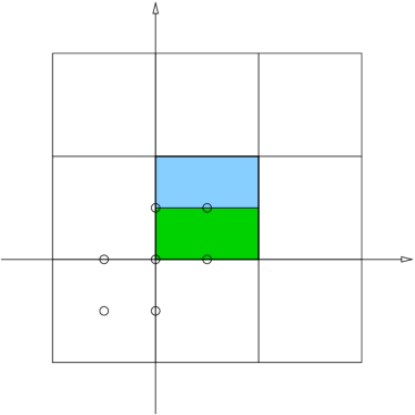
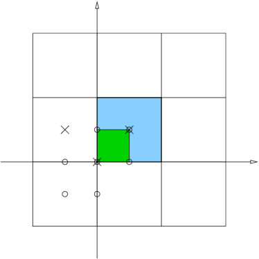
Figure 2: $T^{2}/{\mathbb{Z}}_{2}$ (left panel) and $T^{2}/{\mathbb{Z}}_{4}$ (right panel) orbifolds.

$T^{2}/{\mathbb{Z}}_{3}$ and $T^{2}/{\mathbb{Z}}_{6}$ orbifolds are shown in Fig. 3. The fundamental domain of the torus are all shaded regions while the fundamental domain of the orbifold is only the darkly shaded (green) one. Open circles correspond to fixed points of rotations of $\pi$ and filled circels to rotations of $2\pi/3$. The only fixed point of the rotations of $\pi/3$ is the origin. The images of the fixed points are displayed as well and are easyly seen to be equivalent to its sources by a torus shift.

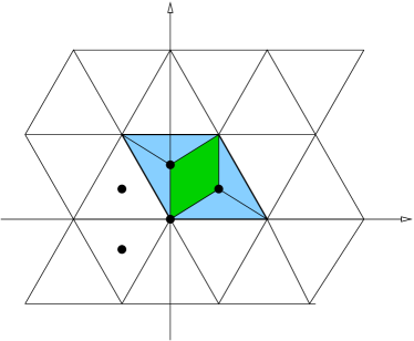
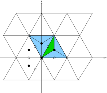
Figure 3: $T^{2}/{\mathbb{Z}}_{3}$ (left panel) and $T^{2}/{\mathbb{Z}}_{6}$ (right panel) orbifolds.

References

- [1] J. Polchinski, “String Theory. Vols. 1 and 2” Cambridge, UK: Univ. Pr. (1998).
- [2] J. D. Lykken, Phys. Rev. D 54 (1996) 3693 [arXiv:hep-th/9603133]; G. Shiu and S. H. Tye, Phys. Rev. D 58 (1998) 106007 [arXiv:hep-th/9805157].
- [3] I. Antoniadis, Phys. Lett. B 246 (1990) 377; I. Antoniadis, C. Munoz and M. Quiros, Nucl. Phys. B 397 (1993) 515 [arXiv:hep-ph/9211309]; I. Antoniadis and K. Benakli, Phys. Lett. B 326 (1994) 69 [arXiv:hep-th/9310151]; I. Antoniadis and M. Quiros, Phys. Lett. B 392 (1997) 61 [arXiv:hep-th/9609209].
- [4] N. Arkani-Hamed, S. Dimopoulos and G. R. Dvali, Phys. Lett. B 429 (1998) 263 [arXiv:hep-ph/9803315]; N. Arkani-Hamed, S. Dimopoulos and J. March-Russell, Phys. Rev. D 63 (2001) 064020 [arXiv:hep-th/9809124]; I. Antoniadis, S. Dimopoulos and G. R. Dvali, Nucl. Phys. B 516 (1998) 70 [arXiv:hep-ph/9710204];
- [5] I. Antoniadis, K. Benakli and M. Quiros, Nucl. Phys. B 583 (2000) 35 [arXiv:hep-ph/0004091].
- [6] E. A. Mirabelli, M. Perelstein and M. E. Peskin, Phys. Rev. Lett. 82 (1999) 2236 [arXiv:hep-ph/9811337]; T. Han, J. D. Lykken and R. J. Zhang, Phys. Rev. D 59 (1999) 105006 [arXiv:hep-ph/9811350]; I. Antoniadis, K. Benakli and M. Quiros, Phys. Lett. B 460 (1999) 176 [arXiv:hep-ph/9905311]; I. Antoniadis and K. Benakli, Int. J. Mod. Phys. A 15 (2000) 4237 [arXiv:hep-ph/0007226]; I. Antoniadis, K. Benakli and M. Quiros, Acta Phys. Polon. B 33 (2002) 2477.
- [7] For a recent review see: M. Quirós, “New ideas in symmetry breaking”, Lectures given at Tasi-02, University of Colorado, CO, USA, June 3-28, 2002, arXiv:hep-ph/0302189.
- [8] L. J. Dixon, J. A. Harvey, C. Vafa and E. Witten, Nucl. Phys. B 261 (1985) 678; L. J. Dixon, J. A. Harvey, C. Vafa and E. Witten, Nucl. Phys. B 274 (1986) 285.
- [9] J. Scherk and J.H. Schwarz, Phys. Lett. B82 (1979) 60; Nucl. Phys. B153 (1979) 61; P. Fayet, Phys. Lett. B159 (1985) 121; Nucl. Phys. B263 (1986) 649.
- [10] A. Pomarol and M. Quiros, Phys. Lett. B 438 (1998) 255 [arXiv:hep-ph/9806263]; I. Antoniadis, S. Dimopoulos, A. Pomarol and M. Quiros, Nucl. Phys. B 544 (1999) 503 [arXiv:hep-ph/9810410]; A. Delgado, A. Pomarol and M. Quiros, Phys. Rev. D 60 (1999) 095008 [arXiv:hep-ph/9812489]; A. Delgado and M. Quiros, Nucl. Phys. B 607 (2001) 99 [arXiv:hep-ph/0103058].
- [11] R. Barbieri, L. J. Hall and Y. Nomura, Phys. Rev. D 63 (2001) 105007 [arXiv:hep-ph/0011311]; N. Arkani-Hamed, L. J. Hall, Y. Nomura, D. R. Smith and N. Weiner, Nucl. Phys. B 605 (2001) 81 [arXiv:hep-ph/0102090].
- [12] N. Arkani-Hamed, A. G. Cohen and H. Georgi, Phys. Lett. B 516 (2001) 395 [arXiv:hep-th/0103135];
- [13] C. A. Scrucca, M. Serone, L. Silvestrini and F. Zwirner, Phys. Lett. B 525 (2002) 169 [arXiv:hep-th/0110073];
- [14] L. Pilo and A. Riotto, Phys. Lett. B 546 (2002) 135 [arXiv:hep-th/0202144].
- [15] R. Barbieri, R. Contino, P. Creminelli, R. Rattazzi and C. A. Scrucca, Phys. Rev. D 66 (2002) 024025 [arXiv:hep-th/0203039];
- [16] S. Groot Nibbelink, H. P. Nilles and M. Olechowski, Phys. Lett. B 536 (2002) 270 [arXiv:hep-th/0203055].
- [17] S. Groot Nibbelink, H. P. Nilles and M. Olechowski, Nucl. Phys. B 640 (2002) 171 [arXiv:hep-th/0205012].
- [18] H. D. Kim, J. E. Kim and H. M. Lee, JHEP 0206 (2002) 048 [arXiv:hep-th/0204132].
- [19] C. A. Scrucca, M. Serone and M. Trapletti, Nucl. Phys. B 635 (2002) 33 [arXiv:hep-th/0203190].
- [20] F. Gmeiner, S. Groot Nibbelink, H. P. Nilles, M. Olechowski and M. Walter, arXiv:hep-th/0208146.
- [21] S. Groot Nibbelink, H. P. Nilles, M. Olechowski and M. G. Walter, arXiv:hep-th/0303101.
- [22] T. Asaka, W. Buchmuller and L. Covi, arXiv:hep-ph/0209144.
- [23] H. M. Lee, arXiv:hep-th/0211126.
- [24] M. B. Green and J. H. Schwarz, Phys. Lett. B 149 (1984) 117.
- [25] P. Horava and E. Witten, Nucl. Phys. B 475 (1996) 94 [arXiv:hep-th/9603142].
- [26] Y. Hosotani, Phys. Lett. B 126 (1983) 309; Annals Phys. 190 (1989) 233.
- [27] K. Fujikawa, Phys. Rev. Lett. 42 (1979) 1195; Phys. Rev. D 21 (1980) 2848 [Erratum-ibid. D 22 (1980) 1499].
- [28] G. von Gersdorff and M. Quiros, Phys. Rev. D 65 (2002) 064016 [arXiv:hep-th/0110132].
- [29] See e.g. M. B. Green, J. H. Schwarz and E. Witten, “Superstring Theory. Vols. 1 and 2” Cambridge, Uk: Univ. Pr. (1987) (Cambridge Monographs On Mathematical Physics).
- [30] See e.g. L. Alvarez-Gaume, “An introduction to anomalies”, HUTP-85/A092 Lectures given at Int. School on Mathematical Physics, Erice, Italy, Jul 1-14 1985.
- [31] J. Wess and B. Zumino, Phys. Lett. B 37 (1971) 95.
- [32] W. A. Bardeen and B. Zumino, Nucl. Phys. B 244 (1984) 421.
- [33] C. G. Callan and J. A. Harvey, Nucl. Phys. B 250 (1985) 427.
- [34] G. von Gersdorff, N. Irges and M. Quiros, Phys. Lett. B 551 (2003) 351 [arXiv:hep-ph/0210134].
- [35] R. L. Schwarzenberger, “N-dimensional crystallography”, Pitman Advanced Pub. Program, London, 1980.
- [36] J. Erler, J. Math. Phys. 35 (1994) 1819 [arXiv:hep-th/9304104]; B. A. Dobrescu and E. Poppitz, Phys. Rev. Lett. 87 (2001) 031801 [arXiv:hep-ph/0102010]; N. Borghini, Y. Gouverneur and M. H. Tytgat, Phys. Rev. D 65 (2002) 025017 [arXiv:hep-ph/0108094].