UT-03-12

hep-th/0305007

AdS Branes Corresponding to Superconformal Defects

Satoshi Yamaguchi

Department of Physics, Faculty of Science, University of Tokyo,
Tokyo 113-0033, Japan.
E-mail: yamaguch@hep-th.phys.s.u-tokyo.ac.jp

Abstract    
We investigate an $AdS_{4}\times L_{2}$ D5-brane in $AdS_{5}\times X_{5}$ space-time, in the context of AdS/dCFT correspondence. Here, $X_{5}$ is a Sasaki-Einstein manifold and $L_{2}$ is a submanifold of $X_{5}$. This brane has the same supersymmetry as the 3 dimensional ${\cal N}=1$ superconformal symmetry if $L_{2}$ is a special Legendrian submanifold in $X_{5}$. In this case, this brane is supposed to correspond to a superconformal wall defect in 4-dimensional ${\cal N}=4$ super Yang-Mills theory. We construct these new string backgrounds and show they have the correct supersymmetry, also in the case with non-trivial gauge flux on $L_{2}$. The simplest new example is $AdS_{4}\times T^{2}$ brane in $AdS_{5}\times S^{5}$. We construct the brane solution expressing the RG flow between two different defects. We also perform similar analysis for an $AdS_{3}\times L_{3}$ M5-brane in $AdS_{4}\times X_{7}$, for a weak $G_{2}$ manifold $X_{7}$ and its submanifold $L_{3}$. This system has the same supersymmetry as 2-dimensional ${\cal N}=(1,0)$ global superconformal symmetry, if $L_{3}$ is an associative submanifold.

1 Introduction

Defect field theories appear in various fields in physics, and an interesting problem. Defect quantum field theories are useful in impurity problem in condensed matter physics. Boundary conformal field theories are special class of defect field theories, and provide the celebrated worldsheet description of D-branes [1]. In the string theory space-time, defect field theories appear as the world-volume low energy theories in the intersecting brane systems [2, 3, 4].

AdS brane/defect CFT (AdS/dCFT) correspondence proposed in [5, 6] is the approach from the AdS/CFT correspondence to these defect field theories. Various aspects of the AdS/dCFT correspondence have been investigated in [7, 8, 9, 10, 11, 12, 13, 14, 15, 16, 17]. The most typical example of the AdS/dCFT is the type IIB one. The string theory side of the correspondence is the IIB supergravity on $AdS_{5}\times S^{5}$ with $AdS_{4}\times S^{2}$ brane whose effective theory is the Dirac-Born-Infeld action. The field theory side is ${\cal N}=4$ super Yang-Mills theory with the wall defect on which the fundamental hyper-multiplet lives [2, 3, 4, 8].

Until now, the $AdS_{m}\times S^{n}$ branes and their corresponding defects have been mainly investigated, but $AdS_{m}\times L_{n}$ branes with non-spherical $L_{n}$ have been less investigated. An $AdS_{m}\times L_{n}$ brane seems to correspond to a nontrivial conformal fixed point of the defect field theory. The RG flows between these fixed points and their brane pictures are good phenomena to see the correspondence.

We study, in this paper, rather general $AdS_{m}\times L_{n}$ type branes. In IIB string theory, we consider an $AdS_{4}\times L_{2}$ brane in $AdS_{5}\times X_{5}$ space-time, where $X_{5}$ is a Sasaki-Einstein manifold. We show that if $L_{2}$ is a special Legendrian submanifold in $X_{5}$, the background preserves the same supersymmetry as 3-dimensional ${\cal N}=1$ superconformal symmetry, as expected. In this analysis, we treat a bent D-brane in AdS part with appropriate gauge flux in $L_{2}$. These are treated in [6, 10] in the $L_{2}=S^{2}$ case. In the case with non-zero flux, the ambient theories of left and right side of the defect are distinct.

The most simple non-trivial example of the special Legendrian submanifold is appropriately embedded $T^{2}$. We investigate $AdS_{4}\times T^{2}$ brane and its corresponding defect CFT. Especially, this CFT can flow to the corresponding CFT of $AdS_{4}\times S^{2}$ brane. We construct the solution of the flow in the brane picture.

We also consider $AdS_{3}\times L_{3}$ M5-brane in $AdS_{4}\times X_{7}$ space-time, where $X_{7}$ is a weak $G_{2}$ manifold. We show that if $L_{3}$ is an associative submanifold, this background has the same supersymmetry as 2-dimensional global superconformal symmetry, as expected. In this analysis, the D-brane can bend in $AdS_{4}$ and admit appropriate 3-form flux at the same time. In this system, the ambient theories of left and right of the defect are distinct as suggested in [6] in the case with $L_{3}=S^{3}$ in $AdS_{4}\times S^{7}$.

The construction of this paper is as follows: Section 2 discuss the supersymmetry of IIB $AdS_{4}\times L_{2}$ brane in $AdS_{5}\times X_{5}$. In section 3, we treat the $AdS_{4}\times T^{2}$ brane, and its flow to $AdS_{4}\times S^{2}$ brane. In section 4, we consider the supersymmetry of $AdS_{3}\times L_{3}$ M5-brane in $AdS_{4}\times X_{7}$ background of M-theory. Section 5 is devoted to conclusions and discussions. We write some definitions and the proof of some formulas in the appendix.

2 IIB $AdS_{4}\times L_{2}$ D5-brane in $AdS_{5}\times X_{5}$

In this section, we study the remaining supersymmetry in the presence of the $AdS_{4}\times L_{2}$ D5-brane in $AdS_{5}\times X_{5}$ space-time of IIB theory. In this paper, we consider the general Sasaki-Einstein manifold $X_{5}$, and the general special Legendrian submanifold $L_{2}$ in $X_{5}$. We also includes the gauge flux on the brane in $L_{2}$ that makes the AdS brane bend. We show that there are the same amount of the supersymmetry as 3-dimensional superconformal symmetry as expected, by using the probe approximation. The analysis in this section is generalisation of the analysis of $AdS_{4}\times S^{2}$ brane in [10] to general special Legendrian submanifold $L_{2}$.

In order to perform this analysis, we first review the construction of the Killing spinors in $AdS_{5}\times X_{5}$ background. This type of backgrounds have been investigated in [18, 19, 20, 21, 22]. Next, we use the kappa symmetry projection to determine the surviving supersymmetry in the presence of $AdS_{4}\times L_{2}$ D5-brane.

2.1 Supersymmetry of the closed string background

Let us first describe the $AdS_{5}\times X_{5}$ solution in 10 dimensional IIB supergravity and fix the convention. We only turn on the metric and the 5-form field strength $F^{(5)}$ in IIB supergravity. The Einstein equation can be written as

$$R_{MN}=\frac{1}{4}F^{(5)}_{MPQRS}F^{(5)}_{N}{}^{PQRS},\qquad M,N,\dots=0,\dots,9.$$ (2.1)

The Bianchi identity for $F^{(5)}$ and self-duality are also required. The metric for the $AdS_{5}\times X_{5}$ is described as

$$ds^{2}=dr^{2}+e^{-2r}dx^{\mu}dx^{\nu}\eta_{\mu\nu}+g_{mn}dy^{m}dy^{n},$$

$$\mu,\nu=0,1,2,3,\qquad m,n=5,6,7,8,9,\qquad\eta_{MN}={\rm diag}(-1,1,1,\dots),$$ (2.2)

where $g_{mn}$ is the Sasaki-Einstein metric of $X_{5}$ normalised as

$$R_{mn}=4g_{mn}.$$ (2.3)

We can always rescale $g_{mn}$ so that Eq.(2.3) is satisfied, if $X_{5}$ is an Einstein manifold with a positive cosmological constant. We set the vielbein $e^{a^{\prime}},\ a^{\prime}=0,1,2,3,4$ of $AdS_{5}$ space-time as

$$e^{p}:=e^{-r}dx^{p},\ (p=0,1,2,3),\qquad e^{4}:=dr,$$ (2.4)

and we denote by $e^{a},\ (a=5,\dots,9)$ the vielbein for the metric $g_{mn}$ of $X_{5}$ space. In this notation, the solution of 5-form can be written as

$$F^{(5)}=4(e^{0}e^{1}e^{2}e^{3}e^{4}+e^{5}e^{6}e^{7}e^{8}e^{9}).$$ (2.5)

Actually, the solution (2.2)(2.5) can have a parameter; the radius of $AdS_{5}$ (or $X_{5}$). In this paper, however, we set the radius to be $1$ because it is irrelevant in the analyses below.

Next, we turn to the Killing spinors. The supersymmetry condition of the gravitino in the background of the metric and the 5-form is expressed as

$$\partial_{A}\epsilon+\frac{1}{4}\omega_{A}{}^{BC}\Gamma_{BC}\epsilon+\frac{i}{2^{4}\times 5!}F^{(5)}_{BCDEF}\Gamma^{BCDEF}\Gamma_{A}\epsilon=0,\qquad\partial_{A}:=(e^{-1})^{M}_{A}\frac{\partial}{\partial x^{M}},$$

$$(A,B,\dots=0,1,\dots,9),$$ (2.6)

where $\epsilon=\epsilon_{L}+i\epsilon_{R}$ is the parameter of the supersymmetry, and $\epsilon_{L,R}$ ’s are Majorana-Weyl spinors with positive chirality. The dilatino condition is trivially satisfied in this case. If we insert the form (2.5) to eq.(2.6), we obtain the form

$$\partial_{A}\epsilon+\frac{1}{4}\omega_{A}{}^{BC}\Gamma_{BC}\epsilon+\frac{i}{2}\Gamma^{01234}\Gamma_{A}\epsilon=0.$$ (2.7)

In this equation, the torsionless spin connection of $AdS_{5}$ becomes $\omega^{p4}=-\omega^{4p}=-e^{p},\ (p=0,1,2,3)$ and other components are $0$. We also denote the spin connection of $X_{5}$ by $\omega^{ab},\ (a,b=5,\dots,9)$ which satisfies $de^{a}+\omega^{ab}e^{b}=0$.

To solve the equation (2.7), we decompose $\epsilon$ in the same way as [23]

$$\epsilon=\epsilon_{+}+\epsilon_{-},\qquad i\Gamma^{0123}\epsilon_{\pm}=\pm\epsilon_{\pm}.$$ (2.8)

Then, eq.(2.7) becomes

$$\frac{\partial}{\partial r}\epsilon_{\pm}\pm\frac{1}{2}\epsilon_{\pm}=0,$$

$$\frac{\partial}{\partial x^{p}}\epsilon_{+}+e^{-r}\Gamma_{4p}\epsilon_{-}=0,\qquad\frac{\partial}{\partial x^{p}}\epsilon_{-}=0,\qquad p=0,1,2,3,$$

$$\partial_{a}\epsilon_{\pm}+\frac{1}{4}\omega_{a}{}^{bc}\Gamma_{bc}\epsilon_{\pm}\pm\frac{1}{2}\Gamma_{4a}\epsilon_{\pm}=0,\qquad a,b,c=5,\dots,9.$$ (2.9)

It is convenient to take the 10 dimensional gamma matrices $\Gamma_{A},\ \{\Gamma_{A},\Gamma_{B}\}=2\eta_{AB}$ as the following form.

$$\Gamma^{a^{\prime}}=\gamma^{a^{\prime}}\otimes\mathbf{1}\otimes\sigma_{1},\qquad\Gamma^{a}=\mathbf{1}\otimes\gamma^{a}\otimes\sigma_{2},\qquad\Gamma^{11}=\mathbf{1}\otimes\mathbf{1}\otimes\sigma_{3},$$ (2.10)

where $\gamma^{a^{\prime}},\ a^{\prime}=0,1,2,3,4$ are $4\times 4$ gamma matrices for SO(4,1), and $\gamma^{a},\ a=5,\dots,9$ are $4\times 4$ gamma matrices for SO(5). These gamma matrices satisfy the relations

$$\{\gamma^{a^{\prime}},\gamma^{b^{\prime}}\}=\eta^{a^{\prime}b^{\prime}},\qquad\{\gamma^{a},\gamma^{b}\}=\delta^{ab},\qquad\gamma^{4}=i\gamma^{0123},\qquad\gamma^{56789}=\mathbf{1}.$$ (2.11)

In eqs.(2.10), we also use the Pauli matrices $\sigma_{j},\ j=1,2,3$. By using these notations, the equation (2.9) can be solved as

$$\epsilon=\lambda\otimes\chi_{-}\otimes\binom{1}{0},$$ (2.12)

$$\lambda=e^{\frac{1}{2}r}\zeta_{-}+e^{-\frac{1}{2}r}\left(x^{p}\gamma_{p4}\zeta_{-}+\zeta_{+}\right),\qquad p=0,1,2,3,$$ (2.13)

$$\zeta_{\pm}:(\text{4 component constant spinor}),\qquad i\gamma^{0123}\zeta_{\pm}=\pm\zeta_{\pm},$$ (2.14)

$$\partial_{a}\chi_{-}+\frac{1}{4}\omega_{a}{}^{bc}\gamma_{bc}\chi_{-}+\frac{i}{2}\gamma_{a}\chi_{-}=0.$$ (2.15)

Eq.(2.15) implies that $\chi_{-}$ is a real Killing spinor in $X_{5}$. It is known that if and only if $X_{5}$ is a Sasaki-Einstein manifold, there is a real Killing spinor [24].

In summary, we write down the Killing spinors of $AdS_{5}\times X_{5}$ in this subsection. These Killing spinors exist only when $X_{5}$ is a Sasaki-Einstein manifold. We consider $AdS_{4}\times L_{2}$ D5-branes in this background and their supersymmetry in the next subsection.

2.2 Supersymmetry of D-brane background

Let us introduce an $AdS_{4}\times L_{2}$ D5-brane into the background considered in the previous subsection. We show that this system has the same amount of the supersymmetry as the 3-dimensional ${\cal N}=1$ superconformal symmetry, as expected.

As in [25, 26, 27, 28, 29, 30, 10], the surviving Killing spinors when we put the D-brane should satisfy

$$\Gamma\epsilon=\epsilon,$$ (2.16)

where $\Gamma$ is the matrix used for the kappa symmetry projection. The matrix $\Gamma$ for a IIB D$p$-brane can be written as

$$d^{p+1}\xi\Gamma=-e^{-\Phi}(-\det(G_{\text{ind}}+{\cal F}))^{-1/2}e^{{\cal F}}{\cal X}|_{(p+1)\text{-form}},$$ (2.17)

$${\cal X}:=\sum_{n}\frac{1}{(2n)!}d\xi^{i_{2n}}\dots d\xi^{i_{1}}\Gamma_{\langle i_{1}i_{2}\dots i_{2n}\rangle}K^{n}(-i),$$ (2.18)

$$\Gamma_{\langle i_{1}i_{2}\dots i_{s}\rangle}:=\frac{\partial X^{M_{1}}}{\partial\xi^{i_{1}}}\dots\frac{\partial X^{M_{s}}}{\partial\xi^{i_{s}}}e_{M_{1}}^{A_{1}}\dots e_{M_{s}}^{A_{s}}\Gamma_{A_{1}\dots A_{s}},$$ (2.19)

where $\xi^{i}$ are the world-volume coordinates, $\Phi$ is the dilaton, $G_{\text{ind}}$ is the induced metric, ${\cal F}=F-B$ is the linear combination of the NSNS B-field and the world-volume gauge field, and $K$ is the charge conjugation $K\epsilon=\epsilon^{c}$.

The brane configuration treated here is described as follows. First, we set the world-volume coordinate as $\xi^{i},\ i=0,1,2,4,5,6$, and take the static gauge (use the space-time coordinate in eq.(2.2))

$$x^{j}=\xi^{j},\quad(j=0,1,2),\qquad r=\xi^{4}.$$ (2.20)

We use $x^{0,1,2},r$ as both space-time and world-volume coordinates. Secondly, we consider the situation where the $AdS$ part of the D-brane bend as $x^{3}=Me^{r}$, where $M$ is a constant. Thirdly, the immersion $(\xi^{5},\xi^{6})\to X_{5}$ is a special Legendrian immersion, and its image is $L_{2}$. Then the induced metric becomes

$$(G_{\text{ind}})_{ij}d\xi^{i}d\xi^{j}=(1+M^{2})dr^{2}+e^{-2r}dx^{\alpha}dx^{\beta}\eta_{\alpha\beta}+G_{pq}d\xi^{p}d\xi^{q},\qquad(\alpha,\beta=0,1,2,\quad p,q=5,6),$$

$$G_{pq}:=g_{mn}\frac{\partial y^{m}}{\partial\xi^{p}}\frac{\partial y^{n}}{\partial\xi^{q}},$$ (2.21)

where $G_{pq}$ is the induced metric of $L_{2}$. Note that through this section, we use $G$ as the induced metric of $L_{2}$. The total induced metric are denoted by $G_{\text{ind}}$. Finally, we introduce the world-volume gauge field excitation ${\cal F}=f\sqrt{\det G}d\xi^{5}d\xi^{6}$ , where $f$ is a constant. Then the DBI determinant becomes

$$-\det(G_{\text{ind}}+{\cal F})=(1+M^{2})e^{-6r}\det(G+{\cal F})=(1+M^{2})(1+f^{2})e^{-6r}\det G.$$ (2.22)

In the above D-brane configuration, the matrix $\Gamma$ in eq.(2.17)-(2.19) becomes

$$\Gamma=\left[(1+M^{2})(1+f^{2})\det G\right]^{-1/2}i\Gamma_{012}(\Gamma_{4}+M\Gamma_{3})\left[\Gamma_{\langle 56\rangle}K+f\sqrt{\det G}\right].$$ (2.23)

Now, let us consider the equation $\Gamma\epsilon=\epsilon$ for the Killing spinors $\epsilon$. We will show that half of the $\epsilon$ satisfy this equation when we set appropriate relation between $f$ and $M$. The key formula for this analysis is

$$\frac{\partial y^{m}}{\partial\xi^{5}}\frac{\partial y^{n}}{\partial\xi^{6}}e^{a}_{m}e^{b}_{n}\gamma_{ab}\chi_{-}^{c}=\sqrt{\det G}\chi_{-},$$ (2.24)

for a special Legendrian submanifold $L_{2}$ and a real Killing spinor $\chi_{-}$ of $X_{5}$ with certain phase. We will show eq.(2.24) in appendix A.2. If we use eq.(2.24), what we should show is

$$\lambda=\Gamma^{\prime}\lambda:=\frac{1}{\sqrt{(1+M^{2})(1+f^{2})}}(\gamma_{3}-\gamma_{4}M)(\lambda^{c}+f\lambda),$$

$$\lambda:=e^{-\frac{1}{2}r}(-x^{\alpha}\gamma_{\alpha}\zeta_{-}+\zeta_{+})+e^{+\frac{1}{2}r}(1-M\gamma_{3})\zeta_{-},$$

$$\lambda^{c}:=e^{-\frac{1}{2}r}(x^{\alpha}\gamma_{\alpha}\zeta_{-}^{c}+\zeta_{+}^{c})+e^{+\frac{1}{2}r}(1+M\gamma_{3})\zeta_{-}^{c}.$$ (2.25)

$\Gamma^{\prime}\lambda$ can be expanded as

$$\Gamma^{\prime}\lambda=\frac{1}{\sqrt{(1+M^{2})(1+f^{2})}}\Bigg{[} e^{-\frac{1}{2}r}\Big{\{}-x^{\alpha}\gamma_{\alpha}(\gamma_{3}\zeta_{-}^{c}-M\zeta_{-}^{c}-f\gamma_{3}\zeta_{-}-fM\zeta_{-})$$

$$\qquad\qquad+(\gamma_{3}\zeta_{+}^{c}+M\zeta_{+}^{c}+f\gamma_{3}\zeta_{+}-fM\zeta_{+})\Big{\}}$$

$$+e^{\frac{1}{2}r}(1+M^{2})(\gamma_{3}\zeta_{-}^{c}+f\gamma_{3}\zeta_{-})\Bigg{]}.$$ (2.26)

From this equation, we obtain the following results. First, if we want a supersymmetry, the bending $M$ and the gauge flux $f$ must satisfy the relation $f=-M$. Next, if this relation is satisfied, the surviving Killing spinors are the ones with $\gamma_{3}\zeta_{-}^{c}=\zeta_{-},\quad\gamma_{3}\zeta_{+}^{c}=\zeta_{+}$. The number of remaining supercharges is $4$ in general. This is the same number as the 3-dimensional ${\cal N}=1$ superconformal symmetry.

Let us check this brane configuration actually satisfies the field equation. The bosonic part of the D5-brane action on this background is

$$I=-\int d^{6}\xi\sqrt{-\det(G_{\text{ind}}+{\cal F})}-\int{\cal F}\wedge C^{(4)},$$ (2.27)

where $C^{(4)}$ is the RR 4-form potential $dC^{(4)}=F^{(5)}$. If we take the static gauge (2.20), the remaining fields are $x^{3},\ y^{m},\ {\cal A}$; ${\cal A}$ is the world-volume gauge field ${\cal F}=d{\cal A}$. The $y^{m}$ and ${\cal A}$ are easily checked to satisfy the field equation. Note that we use here the fact that a special Legendrian submanifold is a minimal submanifold . The equation of motion for $x^{3}$, after we insert the solution ${\cal F}$ and $y^{m}$ and anzats $x^{3}=x^{3}(r)$, becomes

$$\frac{\partial}{\partial r}\left[\sqrt{(1+M(r)^{2})(1+f^{2})\det G}e^{-5r}(1+M(r)^{2})^{-1}\frac{\partial x^{3}}{\partial r}\right]-4f\sqrt{\det G}e^{-4r}=0,$$ (2.28)

$$M(r):=e^{-r}\frac{\partial x^{3}}{\partial r}.$$ (2.29)

We can easily check that $x^{3}(r)=-fe^{r}$ is a solution of this equation of motion.

3 $AdS_{4}\times T^{2}$ brane and its flow to $AdS_{4}\times S^{2}$

In this section, we explain a nontrivial example of special Legendrian submanifolds in $S^{5}$: appropriately embedded $T^{2}$. Many examples of special Legendrian submanifolds in $S^{5}$ (which has one to one correspondence to special Lagrangian cones in $\mathbb{C}^{3}$) are shown in [31, 32]. Among them, we consider here the simplest non-trivial one. In this section, we limit ourselves to the case with $M=f=0$ for simplicity.

The precise immersion of this $T^{2}\to S^{5}$ are described as follows. We parametrise $S^{5}$ by $(z_{1},z_{2},z_{3})\in\mathbb{C}^{3},\quad|z_{1}|^{2}+|z_{2}|^{2}+|z_{3}|^{2}=1$. Then, the special Legendrian $T^{2}$ can be expressed as

$$z_{j}=\frac{1}{\sqrt{3}}e^{i\theta_{j}},\quad j=1,2,3,\qquad\theta_{1}+\theta_{2}+\theta_{3}\equiv 0\mod{2\pi}.$$ (3.1)

The corresponding defect CFT is expected as follows. First consider D3-D5 system described in table 1.

	0	1	2	3	4–9
D3	$\bigcirc$	$\bigcirc$	$\bigcirc$	$\bigcirc$	$\times$
D5	$\bigcirc$	$\bigcirc$	$\bigcirc$	$\times$	$\tilde{L}$

Table 1: The D3-D5 configuration considered here. “$\bigcirc$” means “extended” and “$\times$” means “not extended”. The D5-brane is wrapped on the special Lagrangian submanifold $\tilde{L}$ in 4–9 directions.

The number of D3-branes is $N$, and that of D5-brane is one. In 4–9 directions, the D5-brane is wrapped on a special Lagrangian submanifold $\tilde{L}$; This $\tilde{L}$ is described as the cone over the special Legendrian $T^{2}$. On the other hand, all $N$ D3-branes sit at the tip (singularity) of $\tilde{L}$ in 4–9 direction. Consider the near horizon region of the supergravity solution of D3-branes in this configuration. In this region, the space-time becomes $AdS_{5}\times S^{5}$ and the D5-brane (treated as a probe) becomes $AdS_{4}\times T^{2}$ brane in this space-time. This is the background of the string theory side of the correspondence.

Next, the theory of the field theory side will be obtained as the low energy theory on the D3-branes. This theory includes 2 sectors: 3-3 string sector and 3-5 string sector. Low energy theory of 3-3 string sector is 4-dimensional ${\cal N}=4$ U($N$) super Yang-Mills theory as usual. The 3-5 string sector and its coupling to 3-3 string sector characterise the defect conformal field theory. Because the D3-branes sit at the singularity of the D5-brane, the theory of 3-5 string is singular. This makes it difficult to describe the low energy theory. We postpone this analysis to the future work.

Now, we have two kinds of defects in the ambient theory ${\cal N}=4$ super Yang-Mills theory; one (we call it “$S^{2}$ defect”) corresponds to $AdS_{4}\times S^{2}$ brane, and the other (we call it “$T^{2}$ defect”) corresponds to $AdS_{4}\times T^{2}$ brane. Let us consider here the relation between $S^{2}$ defect and $T^{2}$ defect. If there is some relation between these two defects, it might give a hint on the description of $T^{2}$ defect since the theory of $S^{2}$ defect is known [2, 3, 4, 8].

In order to see the renormalization group flow of $S^{2}$ defect and $T^{2}$ defect, we consider here the g-function in the point of view of the $AdS$ brane[13]. In the present case, the g-function at each fixed point is proportional to the area of $S^{2}$ or $T^{2}$. The ratio of g-function of $T^{2}$ defect ($g_{T^{2}}$) and that of $S^{2}$ defect ($g_{S^{2}}$) becomes

$$\frac{\ln g_{T^{2}}}{\ln g_{S^{2}}}=\frac{\pi}{\sqrt{3}}>1.$$ (3.2)

Therefore, $g_{T^{2}}>g_{S^{2}}$ is satisfied and the RG flow from $S^{2}$ defect to $T^{2}$ defect is forbidden. On the other hand, the RG flow from $T^{2}$ defect to $S^{2}$ defect may exist. In the rest of this section, we show that this $T^{2}\to S^{2}$ flow can be described in the $AdS$ brane side.

The key of this flow is the existence of the special Lagrangian manifold which is non-singular and asymptotically $T^{2}$ cone. This special Lagrangian submanifold $\tilde{L}_{\mu}$ in $\mathbb{C}^{3}=\{(z_{1},z_{2},z_{3})\}$ can be described as

$$z_{2}=\bar{z}_{1}e^{-i\alpha},\qquad z_{3}=\sqrt{|z_{1}|^{2}+\mu^{2}}e^{i\alpha}-\mu,\qquad z_{1}\in\mathbb{C},\qquad e^{i\alpha}\in S^{1},$$ (3.3)

where $\mu$ is a real positive deformation parameter. In the region $|z_{1}|\gg\mu$, $\tilde{L}_{\mu}$ asymptotically reach $\tilde{L}=\tilde{L}_{\mu=0}$. On the other hand, around the origin, this submanifold is smooth and can be approximated by a plane.

Let us introduce large number of D3-branes at the origin of $\tilde{L}_{\mu}$ and a D5-brane extended to the direction 0,1,2 and $\tilde{L}_{\mu}$. Consider the near horizon geometry D3-branes. The bulk geometry is $AdS_{5}\times S^{5}$ described by the metric

$$ds^{2}=t^{2}dx^{\mu}dx^{\nu}\eta_{\mu\nu}+t^{-2}(\sum_{j=1}^{3}|dz_{j}|^{2}),$$ (3.4)

where $t=\sqrt{\sum_{j=1}^{3}|z_{j}|^{2}}$. If we define $t=e^{-r}$ and introduce $S^{5}$ coordinates $y^{m}$, the metric is expressed by eq.(2.2). In the UV region (negatively large $r$ or large $t$), $\tilde{L}_{\mu}$ becomes the cone over $T^{2}$, and the D5-brane in eq.(3.4) looks like $AdS_{4}\times T^{2}$. In the IR region (positively large $r$ or small $t$), $\tilde{L}_{\mu}$ becomes a plane (cone over $S^{2}$), and the D5-brane in eq.(3.4) looks like $AdS_{4}\times S^{2}$. Consequently, this brane configuration expresses the flow from $T^{2}$ defect to $S^{2}$ defect. The image of this flow is illustrated in figure 1.

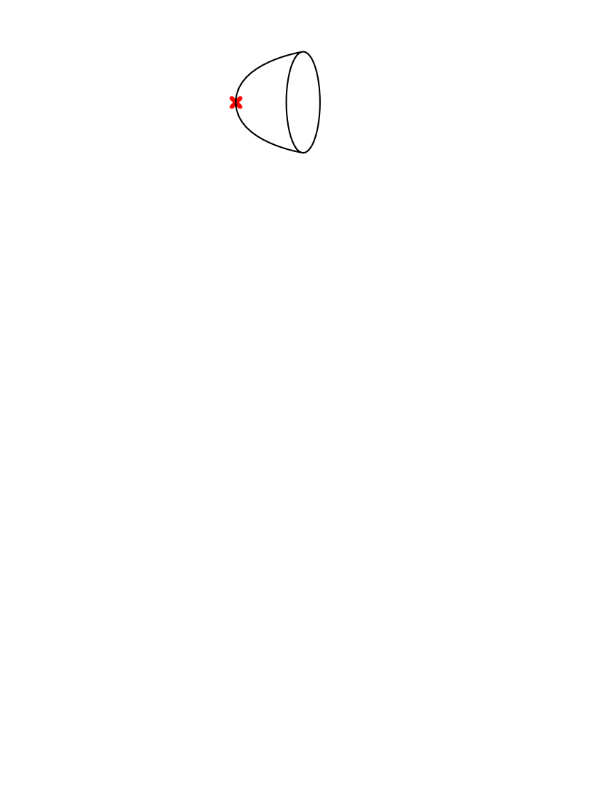
(a)	(b)	(c)

Figure 1: The image of the flow from $T^{2}$-brane to $S^{2}$-brane. (a) UV limit: The D3-branes are sitting at the tip of the $T^{2}$ cone. In the near horizon limit, the D5-brane becomes $AdS_{4}\times T^{2}$ and corresponds to $T^{2}$ defect. (b) Intermediate scale: The defect theory has the RG flow. (c) IR limit: The D3-branes are sitting on a flat D5-brane. In the near horizon limit, the D5-brane becomes $AdS_{4}\times S^{2}$ and corresponds to $S^{2}$ defect.

We can show that there is expected amount of supersymmetry in the $AdS_{5}\times S^{5}$ geometry of eq.(3.4) with D5-brane described with eq.(3.3) and extending to 012 direction.

4 $AdS_{3}\times L_{3}$ M5-brane in $AdS_{4}\times X_{7}$

In this section, we perform the similar analysis as section 2 for the $AdS_{3}\times L_{3}$ M5-brane in $AdS_{4}\times X_{7}$ space-time of M-theory. The M-theory background $AdS_{4}\times X_{7}$ is a typical example of Freund-Rubin compactifications [33]. If $X_{7}$ is a weak $G_{2}$ manifold, this background has the supersymmetry. For a review of this type of compactifications, see [34]. These backgrounds have been also investigated in [21, 22] in the context of AdS/CFT correspondence.

In this paper, we consider M5-brane wrapped on $AdS_{3}\times L_{3}$ in above background. This brane background corresponds to a defect CFT: 3-dimensional CFT with scale invariant wall defect. We show that if $L_{3}$ is an associative submanifold in $X_{7}$, the brane background has the same supersymmetry as 2-dimensional ${\cal N}=(1,0)$ global superconformal symmetry, as expected.

4.1 Supersymmetry of the supergravity background

In this section, we review the construction of the Killing spinors of the background $AdS_{4}\times X_{7}$ when $X_{7}$ is a weak $G_{2}$ manifold.

Let us begin with the 11 dimensional supergravity field equations. If we set gravitino to be $0$, the field equation becomes

$$R_{MN}=\frac{1}{2\times 3!}F_{MPQR}F_{N}{}^{PQR}-\frac{1}{6\times 4!}g_{MN}F_{PQRS}F^{PQRS},$$

$$\partial_{M}\sqrt{-g}F^{MNPQ}+\frac{1}{2\times(4!)^{2}}\epsilon^{M_{1}\dots M_{8}NPQ}F_{M_{1}\dots M_{4}}F_{M_{5}\dots M_{8}}=0,$$

$$(M,N,P,Q,\dots=0,1,\dots,10),$$ (4.1)

where $F$ is the 4-form field strength. The metric of $AdS_{4}\times X_{7}$ can be written as

$$ds^{2}=dr^{2}+e^{-4r}dx^{\mu}dx^{\nu}\eta_{\mu\nu}+g_{mn}dy^{m}dy^{n},\quad(\mu,\nu=0,1,2,3,\quad m,n=4,\dots,10),$$ (4.2)

where $g_{mn}$ is the weak $G_{2}$ metric of $X_{7}$ which is normalised as $R_{mn}=6g_{mn}$. We set the vielbein $e^{a^{\prime}},\ a^{\prime}=0,1,2,3$ of $AdS_{4}$ space-time as

$$e^{3}=dr,\ e^{p}=e^{-2r}dx^{p},\qquad(p=0,1,2),$$ (4.3)

and we denote the vielbein of $X_{7}$ as $e^{a},\ (a=4,\dots,10)$. The solution of the 4-form can be written with these notations as

$$F=6e^{0}e^{1}e^{2}e^{3}.$$ (4.4)

The solution (4.2),(4.4) can have a parameter (“radius”), but we set it $1$ as in the IIB case.

Now, let us turn to the Killing spinor analysis. The gravitino condition of the SUSY parameter (Majorana spinor) $\epsilon$ in a bosonic background can be expressed as

$$\partial_{A}\epsilon+\frac{1}{4}\omega_{A}{}^{BC}\Gamma_{BC}\epsilon+\frac{1}{288}F_{BCDE}\Gamma_{A}{}^{BCDE}\epsilon-\frac{1}{36}F_{ABCD}\Gamma^{BCD}\epsilon=0,$$ (4.5)

where $A,B,C,\dots=0,1,\dots,10$ is the 11 dimensional local Lorents indices, and $\omega_{A}{}^{BC}$ is the torsion-free spin connection.

It is convenient to express the 11 dimensional gamma matrices $\Gamma^{A}$ as the form

$$\Gamma_{a^{\prime}}=\gamma_{a^{\prime}}\otimes\mathbf{1},\qquad(a^{\prime}=0,1,2,3),\qquad\Gamma_{a}=\gamma_{(5)}\otimes\gamma_{a},\qquad(a=5,\dots,11),$$ (4.6)

where $\gamma_{a^{\prime}}\ a^{\prime}=0,1,2,3$ are the $4\times 4$ gamma matrices of SO(3,1) and $\gamma_{a}\ a=4,\dots,11$ are the $8\times 8$ gamma matrices of SO(7). Here we also use the SO(3,1) chirality operator $\gamma_{(5)}:=i\gamma^{0123}$. If we write the Killing spinor as $\epsilon=\lambda\otimes\chi$, the Killing spinor equation (4.5) reduces to

$$\partial_{a^{\prime}}\lambda+\frac{1}{4}\omega_{a^{\prime}}{}^{b^{\prime}c^{\prime}}\gamma_{b^{\prime}c^{\prime}}\lambda+i\gamma_{a^{\prime}}\gamma_{(5)}\lambda=0,\quad(a^{\prime},b^{\prime},c^{\prime}=0,1,2,3),$$ (4.7)

$$\partial_{a}\chi+\frac{1}{4}\omega_{a}{}^{bc}\gamma_{bc}\chi-\frac{i}{2}\gamma_{a}\chi=0,\quad(a,b,c=4,\dots,10).$$ (4.8)

Eq.(4.8) implies that $\chi$ is a real Killing spinor of $X_{7}$. $X_{7}$ admits a real Killing spinor if and only if $X_{7}$ is a weak $G_{2}$ manifold.

We need the $AdS_{4}$ part of the spin connection $\omega^{a^{\prime}b^{\prime}}=\omega_{c^{\prime}}{}^{a^{\prime}b^{\prime}}e^{c^{\prime}}$ in order to solve eq.(4.7). The non-zero components of this spin connection are $\omega^{3p}=-\omega^{p3}=2e^{p},\ p=0,1,2$. As in the IIB case, it is convenient to decompose $\lambda=\lambda_{+}+\lambda_{-}$ with $i\gamma_{3}\gamma_{(5)}\lambda_{\pm}=\pm\lambda_{\pm}$. By using these notations, the $AdS_{4}$ part of the Killing spinor equation (4.7) becomes

$$\frac{\partial}{\partial r}\lambda_{\pm}=\mp\lambda_{\pm},\qquad\frac{\partial}{\partial x^{p}}\lambda_{-}=0,\qquad\frac{\partial}{\partial x^{p}}\lambda_{+}+2e^{-2r}\gamma_{3p}\lambda_{-}=0,\qquad p=0,1,2.$$ (4.9)

These equations are easily solved as

$$\lambda_{+}=e^{-r}(2x^{p}\gamma_{p3}\zeta_{-}+\zeta_{+}),\qquad\lambda_{-}=e^{r}\zeta_{-},$$

$$\zeta_{\pm}:(\text{constant 4-component spinor}),\qquad i\gamma_{3}\gamma_{(5)}\zeta_{\pm}=\pm\zeta_{\pm}.$$ (4.10)

In summary, we obtained the Killing spinors in $AdS_{4}\times X_{7}$

$$\epsilon=\lambda\otimes\chi,\qquad\lambda=e^{-r}(2x^{p}\gamma_{p3}\zeta_{-}+\zeta_{+})+e^{r}\zeta_{-},$$ (4.11)

where $\zeta_{\pm}$ is constant 4-component spinors with $i\gamma_{3}\gamma_{(5)}$ eigenvalues $(\pm)$, and $\chi$ is a real Killing spinor in the weak $G_{2}$ manifold $X_{7}$. We consider M5-branes in this background in the next subsection.

4.2 Supersymmetry of the brane background

Let us introduce $AdS_{3}\times L_{3}$ M5-brane to the background considered above for an associative submanifold $L_{3}$ of the weak $G_{2}$ manifold $X_{7}$. For the supersymmetry in the presence of M5-brane, the associated Killing spinors $\epsilon$ must satisfy

$$\Gamma\epsilon=\epsilon,$$ (4.12)

where $\Gamma$ is the matrix for the kappa symmetry projection. This gamma is expressed as [35, 36, 37, 38, 39, 40]

$$\Gamma:=\frac{1}{6!\sqrt{-\det G_{\text{ind}}}}\varepsilon^{j_{1}\dots j_{6}}\left[\Gamma_{\langle j_{1}\dots j_{6}\rangle}+40\Gamma_{\langle j_{1}j_{2}j_{3}\rangle}h_{j_{4}j_{5}j_{6}}\right].$$ (4.13)

We denote here by $h_{j_{1}j_{2}j_{3}}$ the 3-form field strength on the world-volume which is self-dual with respect to the induced metric $G_{\text{ind}}$. We also use the notation $\Gamma_{\langle j_{1}\dots j_{p}\rangle}$ defined in eq.(2.19).

The brane configuration considered here is as follows. We set the world-volume coordinates as $\xi^{i},\ i=0,1,3,4,5,6$, and the configuration is

$$x^{\alpha}=\xi^{\alpha},\quad(\alpha=0,1),\qquad r=\xi^{3},\qquad x^{2}=\frac{1}{2}Me^{2r},\quad(M:\text{ constant}),$$ (4.14)

$$y^{m}=y^{m}(\xi^{4},\xi^{5},\xi^{6}),\quad(\text{associative immersion}).$$ (4.15)

In this case, the induced metric becomes

$$ds^{2}_{\text{ind}}=(1+M^{2})dr^{2}+e^{-4r}(-(dx^{0})^{2}+(dx^{1})^{2})+G_{jk}d\xi^{j}d\xi^{k},$$ (4.16)

$$G_{jk}=g_{mn}\frac{\partial y^{m}}{\partial\xi^{j}}\frac{\partial y^{n}}{\partial\xi^{k}},\qquad(j,k=4,5,6).$$ (4.17)

We also introduce the world-volume self dual 3-form field strength

$$h=\frac{1}{2}f(1+*_{\text{ind}})\sqrt{\det G}d\xi^{4}d\xi^{5}d\xi^{6},$$ (4.18)

where $f$ is a constant and $*_{\text{ind}}$ is the Hodge dual with respect to the induced metric.

In this brane background, the matrix $\Gamma$ becomes

$$\Gamma=-\frac{1}{\sqrt{1+M^{2}}}\Gamma_{01}(M\Gamma_{2}+\Gamma_{3})\frac{1}{\sqrt{\det G}}\Gamma_{\langle 456\rangle}-f\left[\frac{1}{\sqrt{1+M^{2}}}\Gamma_{01}(M\Gamma_{2}+\Gamma_{3})-\frac{1}{\sqrt{\det G}}\Gamma_{\langle 456\rangle}\right].$$ (4.19)

The key formula for the analysis of this equation is

$$\frac{\partial y^{m_{1}}}{\partial\xi^{4}}\frac{\partial y^{m_{2}}}{\partial\xi^{5}}\frac{\partial y^{m_{3}}}{\partial\xi^{6}}e^{a_{1}}_{m_{1}}e^{a_{2}}_{m_{2}}e^{a_{3}}_{m_{3}}\gamma_{a_{1}a_{2}a_{3}}\chi=-i\sqrt{\det G}\chi,$$ (4.20)

for an associative immersion $(\xi^{4},\xi^{5},\xi^{6})\to X_{7}$ and a real Killing spinor $\chi$ of $X_{7}$. The formula (4.20) is proved in appendix B.2. If we use eq.(4.20), the relation $\Gamma_{\langle 456\rangle}\epsilon=-i\sqrt{\det G}\gamma_{(5)}\epsilon$ is satisfied. Then, $\Gamma\epsilon$ reads

$$\Gamma\epsilon=\frac{1}{\sqrt{1+M^{2}}}i\Gamma_{01}(M\Gamma_{2}+\Gamma_{3})\gamma_{(5)}\epsilon-f\left[\frac{1}{\sqrt{1+M^{2}}}\Gamma_{01}(M\Gamma_{2}+\Gamma_{3})+i\gamma_{(5)}\right]\epsilon.$$ (4.21)

At this stage, the problem is reduced to the $AdS_{4}$ part. The relation eq.(4.19) is equivalent to

$$\Gamma^{\prime}\lambda=\lambda,$$ (4.22)

$$\Gamma^{\prime}=\frac{1}{\sqrt{1+M^{2}}}(M\gamma_{3}-\gamma_{2})+f\left[\frac{1}{\sqrt{1+M^{2}}}(M+\gamma_{32})-\gamma_{3}\right]i\gamma_{3}\gamma_{(5)},$$ (4.23)

$$\lambda=e^{-r}(2x^{\alpha}\gamma_{\alpha 3}\zeta_{-}+\zeta_{+})+e^{r}(1+M\gamma_{23})\zeta_{-},\qquad(\alpha=0,1).$$ (4.24)

The Killing spinors satisfying this equation exist only when $f$ and $M$ satisfy the relation

$$f=\frac{M}{1+\sqrt{1+M^{2}}}.$$ (4.25)

In this case, the surviving Killing spinors are parametrised by 4-component spinors $\zeta_{\pm}$ satisfying

$$\gamma_{2}\zeta_{\pm}=-\zeta_{\pm}.$$ (4.26)

Consequently, the number of the remaining supercharges are the same as expected; half of the number of the ones of 3-dimensional ${\cal N}=1$ superconformal symmetry.

5 Conclusion and Discussion

In this paper, we analyse supersymmetric AdS branes in the context of AdS/dCFT correspondence. We construct the string backgrounds for superconformal defects. Especially, we consider the $AdS_{4}\times T^{2}$ brane background and the corresponding defect CFT. We show that there are the RG flow from $T^{2}$ defect to $S^{2}$ defect. We also construct the M-theory AdS/dCFT backgrounds.

Describing the corresponding defect CFT to the $AdS_{4}\times T^{2}$ brane is an interesting problem. This defect CFT will be obtained by considering the low energy theory on the D3-brane at the singularity of the special Lagrangian D5-brane cone. The singular nature of the D5-brane cone is essential in this case. However, it also make this problem difficult. One possible approach is to describe the $T^{2}$ defect as the low energy theory of a known defect. A candidate for this high energy theory is the defect field theory with a certain number of hyper multiplets. This high energy theory corresponds to $AdS_{4}\times(S^{2}\cup S^{2}\cup\dots)$. Consider a set of special Lagrangian planes intersecting at the origin, and deform it so that the tangent cone of the remaining singularity is the $T^{2}$ cone. If one can do this, one find the high energy conformal defect and the operator of the appropriate relevant deformation.

It will be interesting to consider the AdS brane in the decoupling limit from the gravity theory [41, 17]. This produces the AdS/CFT correspondence only in open strings (or open membranes). Especially, in the case of $AdS_{3}\times L_{3}$ M5-brane, the resulting CFT becomes 2-dimensional one, and the conformal symmetry will enhance to infinite dimensions like in the case of ref. [42].

Another interesting related problem is the string theory in AdS in the small radius limit[43, 44, 45, 46]. In this limit, the defect CFT becomes weak coupling and perturbation can be used. In contrast, the supergravity or DBI description becomes wrong in this limit, and the string correction is essential. To consider AdS/dCFT correspondence in this limit will be useful for understanding the strong stringy effect of the string theory.

Acknowledgement

I would like to thank Tohru Eguchi, Yosuke Imamura and Yuji Sugawara for useful discussions and comments.

This work is supported in part by JSPS Research Fellowships for Young Scientists.

Appendix A Sasaki-Einstein manifolds and special Legendrian submanifolds

A.1 Definitions and properties

Let us consider a $(2k-1)$-dimensional Sasaki-Einstein manifold $X$ with metric $g_{mn},\quad(m,n=2,3,\dots,2k)$. We denote the coordinates of $X$ by $y^{m},\ (m=2,3,\dots,2k)$. We fix the normalisation of the metric as

$$R_{mn}=(2k-2)g_{mn}.$$ (A.1)

$X$ has 3 special differential forms: 1-form $\theta$, $(k-1)$-form $A$ and $B$. These forms satisfy

$$\nabla_{m}\theta_{n}+\nabla_{n}\theta_{m}=0,\qquad g^{mn}\theta_{m}\theta_{n}=1,\qquad\nabla_{p}(d\theta)_{mn}=-2g_{pm}\theta_{n}+2g_{pn}\theta_{m},$$ (A.2)

$$\nabla_{m}(A+iB)_{npq}=\nabla_{[m}(A+iB)_{npq]},\qquad d(A+iB)=i^{k}k*(A+iB).$$ (A.3)

The cone $C(X)$ over a Sasaki-Einstein manifold $X$ is a Calabi-Yau manifold. We introduce the radial coordinate $r$, and write the metric of the Calabi-Yau manifold as

$$ds_{CY}^{2}=dr^{2}+r^{2}g_{mn}dy^{m}dy^{n}.$$ (A.4)

Then Kähler form $J_{MN}$ and holomorphic $k$-form $\Omega_{MN\dots}$, $(M,N,\dots=1,2,\dots,2k)$ are expressed as

$$J=rdr\theta+\frac{1}{2}r^{2}d\theta,\qquad\Omega=r^{k-1}dr(A+iB)+\frac{1}{k}r^{k}d(A+iB),$$ (A.5)

where $*_{2k-1}$ means $(2k-1)$ dimensional Hodge dual with respect to the metric $g_{mn}$.

Sasaki-Einstein manifold $X$ has two linearly independent real Killing spinors. A Real Killing spinor $\chi$ satisfies

$$\partial_{c}\chi+\frac{1}{4}\omega_{c}{}^{ab}\gamma_{ab}\chi-\frac{i}{2}\alpha\gamma_{c}\chi=0,\qquad\alpha=\pm 1,$$ (A.6)

$$\partial_{c}\epsilon:=(e^{-1})^{m}_{c}\frac{\partial}{\partial y^{m}},\qquad e^{a}_{m}:(\text{vielbein}),\qquad(e^{-1})^{m}_{c}e^{a}_{m}=\delta^{a}_{c},$$ (A.7)

$$\omega_{c}{}^{ab}:\text{(spin connection)},\qquad\gamma_{c}:\text{(gamma matrices)},\qquad\{\gamma_{a},\gamma_{b}\}=2\delta_{ab}.$$ (A.8)

If $k=$(odd), one real Killing spinor $\chi_{+}$ satisfies (A.6) for $\alpha=+1$ and the other $\chi_{-}$ satisfies (A.6) for $\alpha=-1$. If $k=$(even), both of the real Killing spinors satisfy (A.6) for $\alpha=+1$. This $\alpha=\pm 1$ corresponds to the chirality of the parallel spinor in the Calabi-Yau cone $C(X)$.

The $(k-1)$-dimensional submanifold $L$ in $X$ is called special Legendrian submanifold if

$$A|_{L}={\rm vol}\,L,$$ (A.9)

where $A|_{L}$ is the pullback of $A$ to $L$, and ${\rm vol}L$ is the volume form of $L$. The definition (A.9) is equivalent to

$$B|_{L}=\theta|_{L}=0.$$ (A.10)

There is another equivalent definition. Consider the cone $\tilde{L}$ of $L$.

$$\tilde{L}=\{(r,y)\in C(X)|r\in\mathbb{R}_{+},y\in L\subset X\}.$$ (A.11)

$L$ is a special Legendrian submanifold in $X$, if and only if $\tilde{L}$ is a special Lagrangian submanifold in $C(X)$.

Some properties of special Legendrian submanifolds are also explained in recent papers [47, 48].

A.2 Proof of the formula (2.24)

We denote the vielbein of $C(X)$ by $E^{A},\ A=1,\dots,2k$ and gamma matrices $\Gamma^{A}$. Let us first prove the formula

$$\frac{1}{k!}E^{A_{1}}\dots E^{A_{k}}\Gamma_{A_{1}\dots A_{k}}\psi_{\pm}^{c}|_{\tilde{L}}=\psi_{\pm}{\rm vol}\,\tilde{L},$$ (A.12)

for a special Lagrangian submanifold $\tilde{L}$ in a Calabi-Yau manifold $C(X)$, and parallel spinors $\psi_{\pm}$, when we adjust the phase of these spinors appropriately. Since, the formula (A.12) is invariant under the local rotation, we can show eq.(A.12) in the convenient local frame. We set the local frame so that the holomorphic $k$-form and Kähler form can be written as

$$\Omega=(E^{1}+iE^{k+1})(E^{2}+iE^{k+2})\dots(E^{k}+iE^{2k}),\qquad J=\sum_{j=1}^{k}E^{j}E^{k+j}.$$ (A.13)

In this frame, the two linearly independent parallel spinors $\psi_{\pm}$ is constant spinors defined by

$$(\Gamma^{j}-i\Gamma^{j+k})\psi_{+}=0,\quad(j=1,\dots,k)\qquad\psi_{-}=(\Gamma^{1}+i\Gamma^{k+1})(\Gamma^{2}+i\Gamma^{k+2})\dots(\Gamma^{k}+i\Gamma^{2k})\psi_{+}.$$ (A.14)

By the explicit calculation, we can show

$$\frac{1}{k!}E^{A_{1}\dots A_{k}}\Gamma_{A_{1}\dots A_{k}}\psi_{+}=\psi_{-}\Omega+(\text{terms proportional to }J),$$ (A.15)

$$\frac{1}{k!}E^{A_{1}\dots A_{k}}\Gamma_{A_{1}\dots A_{k}}\psi_{-}=(-1)^{k(k-1)/2}\psi_{+}\bar{\Omega}+(\text{terms proportional to }J).$$ (A.16)

Since the charge conjugation satisfies $(\psi^{c})^{c}=(-1)^{k(k-1)/2}\psi$, we can adjust the phase of $\chi_{+}$ so that the charge conjugation becomes

$$\psi_{+}^{c}=(-1)^{k(k-1)/2}\psi_{-},\qquad\psi_{-}^{c}=\psi_{+}.$$ (A.17)

If we use the equations (A.15),(A.16),(A.17), and the facts $J|_{\tilde{L}}={\rm Im}\,\Omega|_{\tilde{L}}=0$, ${\rm Re}\,\Omega|_{\tilde{L}}={\rm vol}\,L$ for a special Lagrangian submanifold $\tilde{L}$, we obtain the formula (A.12).

In order to prove the formula (2.24) from (A.12), let us introduce the following form of the vielbein and gamma matrices.

$$E^{1}=dr,\quad E^{a}=re^{a},\quad(a=2,\dots,2k),$$

$$\Gamma_{1}=1\otimes\sigma_{1},\qquad\Gamma_{a}=\gamma_{a}\otimes\sigma_{2},\qquad\Gamma_{(5)}=1\otimes\sigma_{3},$$

$$\gamma_{a}:((2k-1)\text{dimensional gamma matrices}),\qquad\sigma_{1,2,3}:(\text{Pauli matrices}).$$ (A.18)

We consider $k=3$ case (which is relevant to our case) below in this section. The parallel spinors $\psi_{\pm}$ of $C(X)$ can be written in terms of the real Killing spinors $\chi_{\pm}$ as $\psi_{-}=\chi_{-}\otimes\binom{0}{1},\ \psi_{+}=\chi_{+}\otimes\binom{1}{0}$. This definition and eq.(A.12) read

$$\frac{1}{2}e^{a}e^{b}\gamma_{ab}\chi_{-}^{c}|_{L}=\chi_{-}{\rm vol}\,L.$$ (A.19)

If we write this equation by the world-volume coordinate $\xi^{5,6}$, we obtain the formula (2.24) (We write in this appendix $L$ and $X$ instead of $L_{2}$ and $X_{5}$).

Appendix B Weak $G_{2}$ manifolds and associative submanifolds

B.1 Definitions and properties

Let us consider a 7-dimensional weak $G_{2}$ manifold $X_{7}$ with metric $g_{mn},\quad(m,n=2,3,\dots,8)$. We denote the coordinates of $X_{7}$ by $y^{m},\ (m=2,3,\dots,8)$. We fix the normalisation of the metric as

$$R_{mn}=6g_{mn}.$$ (B.1)

Weak $G_{2}$ manifold $X_{7}$ has a special 3-form $\Phi$, which satisfies

$$d\Phi=4*\Phi.$$ (B.2)

The cone of $X_{7}$ becomes a Spin(7) holonomy manifold $C(X_{7})$. The metric is

$$ds_{\rm Spin(7)}^{2}=dr^{2}+r^{2}g_{mn}dy^{m}dy^{n}.$$ (B.3)

The Cayley 4-form $\Psi$ of Spin(7) holonomy manifold $C(X_{7})$ becomes

$$\Psi=r^{3}dr\Phi+\frac{1}{4}r^{4}d\Phi$$ (B.4)

The weak $G_{2}$ manifold $X_{7}$ has a real Killing spinor $\chi$ which satisfies

$$\partial_{c}\chi+\frac{1}{4}\omega_{c}{}^{ab}\gamma_{ab}\chi-\frac{i}{2}\gamma_{c}\chi=0,\qquad$$ (B.5)

where we use the same notation as eq.(A.6).

A 3-dimensional submanifold $L_{3}$ of $X_{7}$ called associative submanifold if

$$\Phi|_{L_{3}}={\rm vol}\,L_{3}.$$ (B.6)

An associative submanifold in $X_{7}$ is related to a Cayley submanifold in $C(X_{7})$. Consider the cone $\tilde{L}_{4}$ of $L_{3}$ in $C(X_{7})$. Then, $L_{3}$ is an associative submanifold in $L_{3}$ if and only if $\tilde{L}_{4}$ in $C(X_{7})$ is an Cayley submanifold.

B.2 Proof of the formula (4.20)

We denote the vielbein of $C(X_{7})$ by $E^{A},\ A=1,\dots,8$ and gamma matrices $\Gamma^{A}$. Let us first prove the formula

$$\frac{1}{4!}E^{ABCD}\Gamma_{ABCD}\psi|_{\tilde{L}_{4}}=\psi{\rm vol}\,\tilde{L}_{4},$$ (B.7)

for a Cayley submanifold $\tilde{L}_{4}$ in a Spin(7) holonomy manifold $C(X_{7})$, and a parallel spinor $\psi$. We use in eq.(B.7) the notation $E^{AB\cdots}=E^{A}E^{B}\cdots$. Since, the formula (B.7) is invariant under local rotation, we can show eq.(B.7) in the convenient local frame. We take the local frame in which the Cayley 4-form $\psi$ can be written in the standard form

$$\Psi= E^{1234}+E^{1256}+E^{1278}+E^{1357}-E^{1368}-E^{1458}-E^{1467}$$

$$-E^{2358}-E^{2367}-E^{2457}+E^{2468}+E^{3456}+E^{3478}+E^{5678},$$ (B.8)

where $E^{ABCD}:=E^{A}E^{B}E^{C}E^{D}$. In this frame, the parallel spinor $\psi$ is the constant spinor satisfying

$$\psi=\Gamma^{1234}\psi=\Gamma^{1256}\psi=\Gamma^{1357}\psi=\Gamma^{12345678}\psi.$$ (B.9)

By local Spin(7) transformation, we can take the frame in which the tangent space of Cayley submanifold $\tilde{L}_{4}$ is spanned by $E^{1},E^{2},E^{3},E^{4}$. Note that local Spin(7) transformation does not change the form (B.8) and (B.9). In this frame, left hand side of (B.7) becomes

$$\frac{1}{4!}E^{ABCD}\Gamma_{ABCD}\psi|_{\tilde{L}_{4}} =E^{1234}\Gamma_{1234}\psi=\psi{\rm vol}\,\tilde{L}_{4}.$$ (B.10)

This is the formula (B.7).

In order to show eq.(4.20) from (B.7), we take the frame and gamma matrices of (A.18). The parallel spinor $\psi$ can be written with the real Killing spinor $\chi$ as $\psi=\chi\otimes\binom{1}{0}$ in these notations. Then, eq.(B.7) reduces to

$$\frac{1}{3!}e^{a}e^{b}e^{c}\gamma_{abc}\chi|_{L_{3}}=-i\chi{\rm vol}\,L_{3}.$$ (B.11)

If we rewrite this equation by world-volume coordinate, we obtain the formula (4.20).

References

• [1] J. Polchinski, “Dirichlet-branes and Ramond-Ramond charges,” Phys. Rev. Lett. 75 (1995) 4724–4727, [hep-th/9510017].
• [2] S. Sethi, “The matrix formulation of type IIB five-branes,” Nucl. Phys. B523 (1998) 158–170, [hep-th/9710005].
• [3] O. J. Ganor and S. Sethi, “New perspectives on Yang-Mills theories with sixteen supersymmetries,” JHEP 01 (1998) 007, [hep-th/9712071].
• [4] A. Kapustin and S. Sethi, “The Higgs branch of impurity theories,” Adv. Theor. Math. Phys. 2 (1998) 571–591, [hep-th/9804027].
• [5] A. Karch and L. Randall, “Locally localized gravity,” JHEP 05 (2001) 008, [hep-th/0011156].
• [6] A. Karch and L. Randall, “Open and closed string interpretation of SUSY CFT’s on branes with boundaries,” JHEP 06 (2001) 063, [hep-th/0105132].
• [7] C. Bachas, J. de Boer, R. Dijkgraaf and H. Ooguri, “Permeable conformal walls and holography,” JHEP 06 (2002) 027, [hep-th/0111210].
• [8] O. DeWolfe, D. Z. Freedman and H. Ooguri, “Holography and defect conformal field theories,” Phys. Rev. D66 (2002) 025009, [hep-th/0111135].
• [9] J. Erdmenger, Z. Guralnik and I. Kirsch, “Four-dimensional superconformal theories with interacting boundaries or defects,” Phys. Rev. D66 (2002) 025020, [hep-th/0203020].
• [10] K. Skenderis and M. Taylor, “Branes in AdS and pp-wave spacetimes,” JHEP 06 (2002) 025, [hep-th/0204054].
• [11] A. Karch and E. Katz, “Adding flavor to AdS/CFT,” JHEP 06 (2002) 043, [hep-th/0205236].
• [12] D. Mateos, S. Ng and P. K. Townsend, “Supersymmetric defect expansion in CFT from AdS supertubes,” JHEP 07 (2002) 048, [hep-th/0207136].
• [13] S. Yamaguchi, “Holographic RG flow on the defect and g-theorem,” JHEP 10 (2002) 002, [hep-th/0207171].
• [14] N. R. Constable, J. Erdmenger, Z. Guralnik and I. Kirsch, “Intersecting D3-branes and holography,” hep-th/0211222.
• [15] N. R. Constable, J. Erdmenger, Z. Guralnik and I. Kirsch, “(De)constructing intersecting M5-branes,” hep-th/0212136.
• [16] O. Aharony, O. DeWolfe, D. Z. Freedman and A. Karch, “Defect conformal field theory and locally localized gravity,” hep-th/0303249.
• [17] N. V. Suryanarayana, “The holographic dual of a SUSY vector model and tensionless open strings,” hep-th/0304208.
• [18] L. J. Romans, “New compactifications of chiral $N=2$ $d=10$ supergravity,” Phys. Lett. B153 (1985) 392.
• [19] I. R. Klebanov and E. Witten, “Superconformal field theory on threebranes at a Calabi-Yau singularity,” Nucl. Phys. B536 (1998) 199–218, [hep-th/9807080].
• [20] S. S. Gubser, “Einstein manifolds and conformal field theories,” Phys. Rev. D59 (1999) 025006, [hep-th/9807164].
• [21] B. S. Acharya, J. M. Figueroa-O’Farrill, C. M. Hull and B. Spence, “Branes at conical singularities and holography,” Adv. Theor. Math. Phys. 2 (1999) 1249–1286, [hep-th/9808014].
• [22] D. R. Morrison and M. R. Plesser, “Non-spherical horizons. I,” Adv. Theor. Math. Phys. 3 (1999) 1–81, [hep-th/9810201].
• [23] P. Claus and R. Kallosh, “Superisometries of the AdS $\times$ S superspace,” JHEP 03 (1999) 014, [hep-th/9812087].
• [24] C. Bär, “Real Killing spinors and holonomy,” Commun. Math. Phys. 154 (1993) 509–521.
• [25] M. Cederwall, A. von Gussich, B. E. W. Nilsson and A. Westerberg, “The Dirichlet super-three-brane in ten-dimensional type IIB supergravity,” Nucl. Phys. B490 (1997) 163–178, [hep-th/9610148].
• [26] M. Aganagic, C. Popescu and J. H. Schwarz, “D-brane actions with local kappa symmetry,” Phys. Lett. B393 (1997) 311–315, [hep-th/9610249].
• [27] M. Cederwall, A. von Gussich, B. E. W. Nilsson, P. Sundell and A. Westerberg, “The Dirichlet super-p-branes in ten-dimensional type IIA and IIB supergravity,” Nucl. Phys. B490 (1997) 179–201, [hep-th/9611159].
• [28] E. Bergshoeff and P. K. Townsend, “Super D-branes,” Nucl. Phys. B490 (1997) 145–162, [hep-th/9611173].
• [29] M. Aganagic, C. Popescu and J. H. Schwarz, “Gauge-invariant and gauge-fixed D-brane actions,” Nucl. Phys. B495 (1997) 99–126, [hep-th/9612080].
• [30] E. Bergshoeff, R. Kallosh, T. Ortin and G. Papadopoulos, “Kappa-symmetry, supersymmetry and intersecting branes,” Nucl. Phys. B502 (1997) 149–169, [hep-th/9705040].
• [31] R. Harvey and H. B. Lawson, Jr., “Calibrated geometries,” Acta Math. 148 (1982) 47–157.
• [32] D. Joyce, “Lectures on Calabi-Yau and special Lagrangian geometry,” math.DG/0108088.
• [33] P. G. O. Freund and M. A. Rubin, “Dynamics of dimensional reduction,” Phys. Lett. B97 (1980) 233–235.
• [34] M. J. Duff, B. E. W. Nilsson and C. N. Pope, “Kaluza-Klein supergravity,” Phys. Rept. 130 (1986) 1–142.
• [35] P. S. Howe, E. Sezgin and P. C. West, “Covariant field equations of the M-theory five-brane,” Phys. Lett. B399 (1997) 49–59, [hep-th/9702008].
• [36] M. Aganagic, J. Park, C. Popescu and J. H. Schwarz, “World-volume action of the M-theory five-brane,” Nucl. Phys. B496 (1997) 191–214, [hep-th/9701166].
• [37] P. Pasti, D. P. Sorokin and M. Tonin, “Covariant action for a $D=11$ five-brane with the chiral field,” Phys. Lett. B398 (1997) 41–46, [hep-th/9701037].
• [38] I. Bandos, K. Lechner, A. Nurmagambetov, P. Pasti, D. P. Sorokin and M. Tonin, “Covariant action for the super-five-brane of M-theory,” Phys. Rev. Lett. 78 (1997) 4332–4334, [hep-th/9701149].
• [39] M. Cederwall, B. E. W. Nilsson and P. Sundell, “An action for the super-5-brane in $D=11$ supergravity,” JHEP 04 (1998) 007, [hep-th/9712059].
• [40] I. Bandos, K. Lechner, A. Nurmagambetov, P. Pasti, D. P. Sorokin and M. Tonin, “On the equivalence of different formulations of the M theory five-brane,” Phys. Lett. B408 (1997) 135–141, [hep-th/9703127].
• [41] D. S. Berman and P. Sundell, $AdS_{3}$ OM theory and the self-dual string or membranes ending on the five-brane,” Phys. Lett. B529 (2002) 171–177, [hep-th/0105288].
• [42] J. D. Brown and M. Henneaux, “Central charges in the canonical realization of asymptotic symmetries: An example from three-dimensional gravity,” Commun. Math. Phys. 104 (1986) 207–226.
• [43] A. A. Tseytlin, “On limits of superstring in $AdS_{5}\times S^{5}$,” Theor. Math. Phys. 133 (2002) 1376–1389, [hep-th/0201112].
• [44] A. Karch, “Lightcone quantization of string theory duals of free field theories,” hep-th/0212041.
• [45] A. Dhar, G. Mandal and S. R. Wadia, “String bits in small radius AdS and weakly coupled $N=4$ super Yang-Mills theory. I,” hep-th/0304062.
• [46] A. Clark, A. Karch, P. Kovtun and D. Yamada, “Construction of bosonic string theory on infinitely curved anti-de Sitter space,” hep-th/0304107.
• [47] A. Mikhailov, “Special contact Wilson loops,” hep-th/0211229.
• [48] S. H. Wang, “Compact special Legendrian surfaces in $S^{5}$,” math.DG/0211439.