Late-time dynamics of brane gas cosmology

Abstract

Brane gas cosmology is a scenario inspired by string theory which proposes a simple resolution to the initial singularity problem and gives a dynamical explanation for the number of spatial dimensions of our universe. In this work we have studied analytically and numerically the late-time behaviour of these type of cosmologies taking a proper care of the annihilation of winding modes. This has help us to clarify and extend several aspects of their dynamics. We have found that the decay of winding states into non-winding states behaving like a gas of ordinary non-relativistic particles precludes the existence of a late expansion phase of the universe and obstructs the growth of three large spatial dimensions as we observe today. We propose a generic solution to this problem by considering the dynamics of a gas of non-static branes. We have also obtained a simple criterion on the initial conditions to ensure the small string coupling approximation along the whole dynamical evolution, and consequently, the consistency of an effective low-energy description. Finally, we have reexamined the general conditions for a loitering period in the evolution of the universe which could serve as a mechanism to resolve the brane problem - a problem equivalent to the domain wall problem in standard cosmology - and discussed the scaling properties of a self-interacting network of winding modes taking into account the effects of the dilaton dynamics.

I Introduction

To understand the nature of the initial singularity and the origin of the number of dimensions of our universe are two fundamental problems in cosmology. Is it any physical law that allows the universe to avoid the initial singularity? Why we live in $3+1$ dimensions? Is it, some how, possible to explain dynamically the spatial dimensionality of spacetime? In the standard theory of general relativity the number of dimensions of the cosmological spacetime is not derived from any fundamental law but simply assumed to be four. Moreover, it cannot address the problem of the initial singularity either because it is quite reasonable to believe that Einstein equations will not be valid close to the Planck scale.

An exciting potential resolution of these two issues within the framework of superstring theory was proposed by Brandenberger and Vafa in the late 80’s Brandenberger and Vafa (1989). This proposal is based in a fundamental symmetry of string theory called T-duality which states that the physics of strings in a box of size $R$ do not change if we replace the length of the box by $l^{2}_{st}/R$ (where $l^{2}_{st}$ is the string length). This symmetry is not respected by the standard cosmological equations of general relativity but it is naturally implemented when the dynamics of a dilaton field is properly taking into account Tseytlin and Vafa (1992); Tseytlin (1992).

In this framework the background spacetime has the topology of a torus with nine dimensions, which are assumed to be of equal size, and the dynamics is driven by a gas of fundamental strings. The evolution of the universe is considered to be adiabatic, that is, there is no cosmological production of entropy, and, the string coupling constant is assumed to be small such that an effective tree-level approximation of the string theory is valid. The string gas supports different string states which can be decomposed as combinations of oscillatory modes (stationary vibrating strings), momentum modes (non-stationary strings), and winding modes (strings wrapping around the torus). The T-duality symmetry interchanges winding modes with momentum modes leaving the spectrum of the theory invariant under the inversion of the radius of the torus (the energy of oscillatory modes is independent of the size of the torus). Under this symmetry the temperature of the string gas is also invariant in the sense that it is the same when the size of the universe is $R$ or $l^{2}_{st}/R$. That means that no physical singularity will occur as the radius of the torus is made indefinitely small ($R\ll l_{st}$) avoiding the inherent temperature singularity of standard cosmology.

This scenario also offers a mechanism for explaining an upper bound for the spacetime dimensionality under the assumption of thermal equilibrium. The net cosmological effect of winding modes is to stop expansion even though their energy grows when the volume of space increases. The reason is because they contribute to the expansion with a total negative pressure. The evolution of winding modes can be though as equivalent to that of large classical cosmic strings. If thermal equilibrium is maintained energy from the winding states can be transferred to the rest of the states of the energy spectrum and we can keep the universe expanding. The key observation is to realize that the probability of interaction decreases with the dimensionality of spacetime. As a result, the annihilation of strings with winding number can only be efficient if the number of dimensions of the spacetime is not larger than four. Then, at some point in the evolution, six spatial dimensions of the torus must remain small while the other three become large relative to the string length. Which dimensions grow and which stay small will mostly depend on thermal and quantum fluctuations. These qualitative arguments have been confirmed numerically Sakellariadou (1996); Cleaver and Rosenthal (1995). Some thermodynamical aspects of a string gas and their implications for cosmology have been reviewed in Bassett et al. (2003).

Recently, these ideas have been revived by Brandenberger et al. Alexander et al. (2000) in order to include extended degrees of freedom other than fundamental strings Polchinski (1995, 1996, 1998). In this scenario the early universe is assumed to have $D+1$ spacetime dimensions with an isotropic toroidal topology and filled with a gas consisting of all possible branes with spatial dimension $p<D$ that the spectrum of a particular string theory could admit. Because Dp-branes respect T-duality Sen (1996) the initial singularity problem can also be easily resolved within this extended scenario Alexander et al. (2000) (for a more detailed discussion see Boehm and Brandenberger (2002)). As with fundamental strings, the energy of winding modes of Dp-branes grows with expansion, giving the larger contribution to the total energy of the gas those with the largest $p$, and they also tend to prevent expansion. Assuming thermal equilibrium as well, the cosmology of brane gases may also provide an explanation for the dimensionality of spacetime by an analogous mechanism of self-annihilation of winding states. Modes with larger $p$ are more massive and they must decay first allowing only $2p+1$ spatial dimensions to grow. The late-time evolution will be dominated by the winding modes with the lower spatial dimension ($p=1$). Then, a hierarchy of small dimensions is generated and the observed dimensionality of our universe can be again explained. Generalisations of brane gas models to manifolds with non-toroidal topology and to anisotropic backgrounds have been studied in Easson (2001); Easther et al. (2002a) and Watson and Brandenberger (2003), respectively. Attends to extend and discuss these type of cosmological scenarios by including fundamental degrees of freedom of 11-dimensional M-theory have been given in Easther et al. (2002b); Alexander (2002).

Even though the string considerations of Brandenberger and Vafa (1989) generalise quite easily to branes gases, they face a problem similar to the standard domain wall problem of cosmological models admitting the spontaneous breaking of a discrete symmetry in the early universe Zeldovich et al. (1974); Vilenkin and Shellard (1994). Causality indicates that despite an efficient annihilation of the winding states at least one Dp-brane across a Hubble volume should have survived. As with domain walls defects, the presence of even only one brane in our present horizon with an energy larger than the electroweak scale would have introduced fluctuations in the temperature of the microwave background radiation incompatible with current experimental bounds. This observation pose a severe constraint on cosmological models filled with branes gases. A solution to this new brane problem, proposed in Alexander et al. (2000) and further developed in Brandenberger et al. (2002), is to invoke a sufficiently long period of cosmological loitering Lemaître (1931); Glanfield (1966); Felten and Isaacman (1986); Sahni et al. (1992); Feldman and Evrard (1993) which might have allowed the whole spatial extend of the universe to be in causal contact so the actual absence of branes can be explained by microphysical processes.

The purpose of this work is to clarify and extend previous results on the late-time dynamics of brane gas cosmologies (BGC). In particular, we have been interested to analyse several aspects of the cosmological evolution of this type of scenarios by incorporating the annihilation of brane modes with winding number appropriately. First, we have discussed analytically the qualitative features which are not sensible to the details of the modelling of winding mode decay. We have found that spatial dimensions cannot grow large if the brane states without winding number are produced in the form of ordinary non-relativistic matter. We suggest that this obstruction to explain the dimensionality of the spacetime can be very easily resolved if a gas of non-static branes is considered. Additionally, we have obtained a simple criterion on the initial conditions that guarantee the smallness of the string coupling at all times and, consequently, the consistency of an effective low-energy description for BGC. We have seen, by studying numerically how the dynamics change with respect to the values of some representative parameters, that the particular characteristics of the decay of winding modes mainly affect intermediate stages of the evolution of the universe. Finally, we have been interested to check the robustness of the resolution of the above mentioned brane problem by a phase of loitering and to investigate the scaling properties of a network of self-interacting winding states driven by the dynamics of a dilaton field.

The rest of the paper is organised as follows. In Sec. II we give a brief review of the main ingredients of BGC. Sec. III is divided into two main parts. In the first part we describe with some detail how the process of winding mode decay into small loops without winding number can be modelled. The second part is devoted to investigate the corresponding late-time cosmological dynamics. The conclusions of our analysis are summarised in Sec. IV.

II Cosmology of brane gases

The brane gas scenario assumes that the early universe is filled with a gas in thermal equilibrium containing all the Dp-branes supported by the compactification of 11-dimensional M-theory on $S^{1}$. All the nine spatial dimensions left after compactification are considered to be toroidal and to start expanding adiabatically with an initial size of the order of the string length. The cosmological dynamics of this set up is dictated by the low-energy effective action,

$$S_{B}=-\int d^{D+1}x\,\sqrt{-G}\,\mathrm{e}^{-2\phi}\left[R+4(\nabla_{\mu}\phi)^{2}-\frac{1}{12}H^{2}_{\mu\nu\alpha}\right],$$ (1)

where $D$ are the spatial dimensions, $R$ denotes the scalar curvature corresponding to the metric tensor $G_{\mu\nu}$, $\phi$ represents the dilaton field, which is related with the radius of compactification, and $H_{\mu\nu\alpha}$ is the field strength of a bulk two-form potential $B_{\mu\nu}$. We are going to employ units in which the string length is $l_{st}\sim 1$. The matter source in this scenario is given by a gas of Dp-branes. The dynamics of individual branes with $p$ spatial dimensions embbeded in a $(D+1)$-dimensional bulk spacetime is described by the Dirac-Born-Infeld action Polchinski (1998) (see also Leigh (1989)),

$$S_{p}=T_{p}\int d^{p+1}\xi\,\mathrm{e}^{-\phi}\sqrt{-\mathrm{det}(G_{\alpha\beta}+B_{\alpha\beta}+2\pi\alpha^{\prime}F_{\alpha\beta})},$$ (2)

where $T^{-1}_{p}=\sqrt{\alpha^{\prime}}(2\pi\sqrt{\alpha^{\prime}})^{p}$, $\sqrt{\alpha^{\prime}}$ is the string length $l_{st}$, the set of coordinates $\xi^{\alpha}(\alpha=0,\cdots,p)$ parametrise the D-brane world-volume, $G_{\alpha\beta}$ and $B_{\alpha\beta}$ are the pull-backs of the $(D+1)$-spacetime metric $G_{\mu\nu}$ and the antisymmetric tensor field $B_{\mu\nu}$, respectively, while $F_{\alpha\beta}$ is the field strength of a $U(1)$ gauge field $A_{\mu}$ living on the D-brane. This action includes the dynamics of transverse mode fluctuations, governed by $(D-p)$ world-volume scalar fields, and longitudinal mode fluctuations, described by the gauge field, in addition to winding modes giving the background mass of the brane. In the standard picture of BGC it is assumed that brane mode fluctuations are small and only winding modes dominate the cosmological dynamics. The mass energy of these modes is given by (see for instance Maggiore and Riotto (1999); Boehm and Brandenberger (2002)),

$$E^{(p)}_{w}=\tau_{p}\,Vol_{p}.$$ (3)

with $\tau_{p}=T_{p}/g$ a re-scaled brane tension, $Vol_{p}$ the physical spatial volume of the brane, and $g\equiv\exp(\phi)$ the string coupling which is considered to be small. The equation of state corresponding to winding modes with $p$ spatial dimensions is Alexander et al. (2000); Vilenkin and Shellard (1994),

$$P_{w}^{(p)}=\gamma_{p}E_{w}^{(p)},\textrm{\,\,\, with }\gamma_{p}=-\frac{p}{D}.$$ (4)

In this work we shall restrict our analysis to spatially flat homogeneous and isotropic spacetime backgrounds,

$$ds^{2}=-dt^{2}+\mathrm{e}^{2\lambda(t)}\sum^{D}_{i=1}dx^{2}_{i}.$$ (5)

In Watson and Brandenberger (2003), it was shown that the isotropy of the three large spatial dimensions that remains after the decay of the winding degrees of freedom comes out directly as a consequence of the dynamics. Introducing the new dilaton variable $\varphi=2\phi-D\lambda$, the background equations of motion derived from the total effective action can be written as Tseytlin and Vafa (1992); Tseytlin (1992); Veneziano (1991); Gasperini and Veneziano (2003),

$$\dot{\varphi}^{2}-D\dot{\lambda}^{2} = \mathrm{e}^{\varphi}E,$$

$$\ddot{\varphi}-D\dot{\lambda}^{2} = \frac{1}{2}\,\mathrm{e}^{\varphi}E,$$

$$\ddot{\lambda}-\dot{\varphi}\dot{\lambda} = \frac{1}{2}\,\mathrm{e}^{\varphi}P.$$ (6)

where $E$ and $P$ are the total energy and pressure build on all (winding and non-winding) matter source contributions,

$$E = \sum_{p}E_{w}^{(p)}+E_{nw},$$ (7)

$$P = \sum_{p}\gamma_{p}E_{w}^{(p)}+\gamma E_{nw}.$$ (8)

For non-winding modes we will consider an ordinary equation of state $P_{nw}=\gamma E_{nw}$ with $0\leq\gamma\leq 1$. The above dynamical equations obey an energy conservation law, $\dot{E}+D\dot{\lambda}P=0$, which comes out as a result of the adiabatic approximation Tseytlin and Vafa (1992).

III Late-time dynamics

The early-time dynamics of BGC is quite well understood and it has been extensively discussed Tseytlin and Vafa (1992); Alexander et al. (2000); Bassett et al. (2003); Tsujikawa (2003). In this work we are mainly interested in investigating the late-time dynamics of this type of cosmologies. For that purpose it is fundamental to supplement the field equations given in (6) with an appropriate description of the decay of winding modes into states without winding number. We will assume that all winding states with $p>1$ have already been completely annihilated and six spatial dimensions have been frozen. Then, we can consider that the cosmological evolution is only driven by the dynamics of winding modes with $p=1$ in three spatial dimensions ($D=3$).

III.1 Modelling the decay of winding modes

The cosmological evolution of the winding strings can be thought as analogous to that of a network configuration of long cosmic strings in an expanding universe with toroidal topology Bennett (1986a, b); Vilenkin and Shellard (1994); Brandenberger (1994). At time $t$ the total energy of a gas of $N_{w}$ winding modes with individual mass-energy $\tau R(t)$, recall Eq. (3), can be expressed as,

$$E_{w}(t)=N_{w}(t)\tau R(t)=\tau l_{c}N_{w}(t)\mathrm{e}^{\lambda(t)}.$$ (9)

The initial physical size of any of the spatial dimensions of the torus, $l_{c}\exp(\lambda(0))$, is usually assumed to be of the order of the string length. Using Eq. (9) one can find an evolution equation for the total energy of the winding string gas,

$$\dot{E}_{w}=\dot{\lambda}E_{w}+\tau R(t)\dot{N}_{w}(t).$$ (10)

The second term represents the loss of energy due to the production of small loops without winding number. If the winding mode decay is negligible the above equation corresponds to the classical conservation equation of an ideal gas of non-interacting strings with equation of state $P_{w}=-E_{w}/3$, recall Eq. (4). Long strings decay into small loop strings through self-interactions. For such a network there exists a characteristic length scale $L_{w}(t)=R/\sqrt{N_{w}}$ which describes the typical separation between the string-like branes. The rate of energy loss by the decay of winding modes into the production of small loops can be roughly approximated by,

$$\left.\dot{E}_{w}\right|_{\mathrm{loop}} \sim -c\cdot\frac{1}{L^{4}_{w}}\cdot\tau^{\prime}L_{l}\cdot V$$ (11)

$$\sim -c\,\tau N^{2}_{w}(t)\left(\frac{L_{l}(t)}{R(t)}\right).$$

The parameter $c$ measures the efficiency of loop production, the space volume is denoted by $V$, and $L_{l}(t)$ represents the typical size of the created loops. The contribution $L^{-4}_{w}$ estimates the number of collisions per unit volume in a network with length scale $L_{w}$ whereas the second contribution, $\tau^{\prime}L_{l}$, expresses the fact that the energy loss has to be proportional to the energy scale at which the small loops are produced. In the last part of the above rate equation, we have assumed that the string tension of the created loops should be similar to that of the winding modes $\tau^{\prime}\sim\tau$. From Eqs. (10) and (11) it is easy to obtain an evolution equation for $N_{w}(t)$,

$$\dot{N}_{w}(t)=-\frac{c}{l^{2}_{c}}L_{l}(t)N^{2}_{w}(t)\mathrm{e}^{-2\lambda(t)}.$$ (12)

Now it is convenient to introduce a dimensionless function of cosmological time, $N_{l}(t)$, in order to write the total energy of small string loops as,

$$E_{l}(t)=N_{l}(t)\tau R(t)\mathrm{e}^{-(1+3\gamma)\lambda(t)}=\tau l_{c}N_{l}(t)\mathrm{e}^{-3\gamma\lambda(t)},$$ (13)

For $\gamma=0$ the produced loops behave like ordinary static matter and for $\gamma=1/3$ as relativistic particles. The function $N_{l}(t)$ describes the production of loops, it is zero if there is no loops at all and constant if they are no longer created. Thus, the rate of change for the total energy of produced loops will be,

$$\dot{E}_{l}=-3\gamma\dot{\lambda}E_{l}+\tau R(t)\dot{N}_{l}(t)\mathrm{e}^{-(1+3\gamma)\lambda(t)}.$$ (14)

The first term corresponds to the variation of energy due to the expansion of the universe and the second to the energy gained through winding mode decay. Within our adiabatic approximation (recall that this assumption is equivalent to the energy conservation equation discussed at the end of Sec. II), we can find an evolution equation for $N_{l}(t)$,

$$\dot{N}_{l}(t)=\frac{c}{l^{2}_{c}}L_{l}(t)N^{2}_{w}(t)\mathrm{e}^{(3\gamma-1)\lambda(t)}.$$ (15)

Obviously, $c=0$ corresponds to no loop creation. Note that in this case the energy density of winding modes simply scales as $\rho_{w}\sim\exp(-2\lambda)$ and, consequently, it should always dominate over ordinary matter or radiation components into the future of a expanding universe.

The field equations (6) can now be cast into a close set of first-order differential equations which completely describes the evolution of the universe during the process of winding mode decay ,

$$\dot{\varphi} = f,$$ (16)

$$\dot{\lambda} = l,$$ (17)

$$\dot{f} = 3l^{2}+\frac{1}{2}\,\mathrm{e}^{\varphi}\left(E_{w}+E_{l}\right),$$ (18)

$$\dot{l} = fl-\frac{1}{6}\,\mathrm{e}^{\varphi}\left(E_{w}-3\gamma E_{l}\right),$$ (19)

$$f^{2} = 3l^{2}+\mathrm{e}^{\varphi}\left(E_{w}+E_{l}\right),$$ (20)

together with Eqs. (9), (12), (13), and (15). Notice that $l$ is nothing but the Hubble parameter.

To complete the description of winding mode annihilation we will have to make an assumption about the formation of small loops. Following Bennett (1986b) (see also Brandenberger et al. (2002)) we will assume the loops are produced with a radius proportional to cosmic time, $L_{l}(t)\sim t$. This will imply that at late times loops are formed with a typical size of the order of the Hubble horizon. Another reasonable possibility would have been to assume that the radius of loops scales with the characteristic length of the winding string network, that is $L_{l}(t)\sim L_{w}$. We have, nevertheless, checked that both cosmological evolutions are not substantially different. All these points will be made more clear in a later section where we will discuss the scaling properties of the winding mode network. Certainly, more sophisticated models to describe the decay of winding modes could be conceived. For instance, one can take into account the possibility of the reconnection of small loops to winding strings and loop decay into gravitational radiation or ordinary matter (relativist or not). However, for our purpose we can keep the description of winding mode annihilation as simple as possible.

III.2 Cosmological dynamics

In the most simple cosmological picture of BGC the universe is assumed to be initially in a state with all its spatial dimensions expanding isotropically, $l>0$, and with a physical size of the order of the string length, $l_{st}\sim 1$. As we have explained, these small toroidal dimensions can only become large if the winding and anti-winding modes can self-annihilate and decay into fundamental string loops or relativistic matter. In what follows we will be interested to explore several dynamical aspects of these cosmological scenarios.

III.2.1 Qualitative analysis

Let us start this section illustrating some general properties of the dynamical evolution of BGC including the effects of winding mode decay but independently of the particular modelling of small loop creation. Consider the two-dimensional phase space spanned by $(f,l)$. The constraint equation (20) in conjunction with the condition of positivity of the total energy restrict the cosmological dynamics to values that satisfy the inequalities

$$f^{2}-3l^{2}\geqslant 0\,\,\,\,\,\mathrm{or}\,\,\,\,\,|l|\leqslant\frac{1}{\sqrt{3}}|f|.$$ (21)

The straight lines $l=\pm f/\sqrt{3}$ correspond to solutions of the equations of motion with zero total energy (that is $E_{w}=E_{l}=0$ except in the exceptional limiting case $\varphi\rightarrow-\infty$ where the total energy can take any finite positive value) passing through the origin. To probe the dynamical character of the fixed point $(f,l)=(0,0)$ it is sufficient to study the time evolution of these special solutions. From Eq. (19) it is straightforward to check that $l$ increases or decreases depending exclusively on the sign of $fl$. In the first and third quadrant of the phase space $l$ must grow and in the second and fourth quadrant it has to diminish. As a consequence, the two straight trajectories lying in the first and fourth quadrant move away from the origin and those in the second and third quadrant move closer to the origin. Since self-consistency demands that there are no trajectories in phase space crossing these special lines, any other trajectory solution of the equations of motion originating in the half left side of phase space approaches the origin asymptotically whereas trajectories that start in the half right side diverge from it, see Fig. 1. Then, the fixed point $(f,l)=(0,0)$ is a saddle point and in fact it is also, as it can be easily shown, the only critical point of the equations of motion. This simple dynamical picture is substantially modified if higher order curvature terms are included in the low-energy effective action Campos (2003).

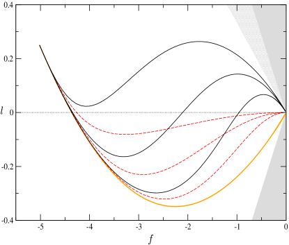
Figure 1: Phase space for $(f,l)$. In the dark grey area ($f^{2}-3l^{2}<0$) the total energy of the matter sources is negative and therefore it is excluded from the dynamical analysis. The light grey dotted wedge, defined by the lines $l=-f/3$ and $l=-f/\sqrt{3}$, is a region where the smallness of the string coupling cannot be guaranteed. We have plotted the numerical solutions of the equations of motion for several values of the physical parameters $c$, the efficiency of the winding mode decay, and $\gamma$, the parameter characterising the equation of state of the loops created. The dashed lines correspond to solutions with $\gamma=0$ whereas the dark continuous lines to solutions with $\gamma=1/3$. In both cases $c$ takes values $(0.1,1.0,10)$ from bottom to top. For comparison we have also included the solution corresponding to no winding mode decay $c=0$ (light continuous line).

Now, let us see that for a given equation of state of the created loops all the solutions of the dynamical equations approach the origin asymptotically close to a particular straight line. In other words, there exists a straight line which is a local solution of the equations of motion near the origin that attracts all other dynamically allowed trajectories in phase space. When the annihilation of winding modes is not taking into account this straight line is $l=f/3$ Tseytlin and Vafa (1992); Alexander et al. (2000), which is in fact a global solution of the equations of motion. Intuitively one should expect that very close to the critical point almost all winding modes have already disappeared and mainly the source energy is in the form of a gas of string loops. In this regime $f$ and $l$ obey two differential equations decoupled from the rest of the variables,

$$\dot{f} \simeq \frac{3}{2}l^{2}+\frac{1}{2}f^{2},$$

$$\dot{l} \simeq fl+\frac{\gamma}{2}\left(f^{2}-3l^{2}\right).$$ (22)

To check our statement we have to look for straight line solutions inside the energetically allowed region, that is solutions of the form $l=\alpha f$ with $\alpha$ being a constant which obeys $|\alpha|\leq 1/\sqrt{3}$. Substituting in the previous two equations we obtain a consistency algebraic equation for $\alpha$,

$$(\alpha+\gamma)(3\alpha^{2}-1)=0.$$ (23)

Apart from the straight global solutions already studied ($l=\pm f/\sqrt{3}$) we get a new solution which depends on the equation of state of the produced loops $l=-\gamma f$. For the static case we get the horizontal line $l=0$ and in the relativistic limit the line $l=-f/3$. Obviously, this local solution does not exist if $|\gamma|>1/\sqrt{3}$. To see that these new special lines are attractors of the dynamics close to the origin we have to analyse the behaviour of small deviations $l=\alpha f+\epsilon$ with $|\epsilon|\ll 1$. Using Eqs. (22) again, the evolution of $\epsilon$ can be determined by the differential equation,

$$\dot{\epsilon}=\left[1-3\alpha(\alpha+\gamma)\right]f\epsilon-\frac{3}{2}(\alpha+\gamma)\epsilon^{2}.$$ (24)

For $\alpha=-\gamma$ this equation reduces to $\dot{\epsilon}=f\epsilon$ and then, noting that $f$ is negative and cannot change sign, it is very easy to see that the absolute value of $\epsilon$ is always a decreasing function of time. To probe the dynamical behaviour of the two other straight lines solutions looks much more subtle because the evolution of $\epsilon$ depends on the value of $\gamma$. Moreover, second order effects will come to dominate at late times and cannot be neglected. In general, one can say that at early times the line $\alpha=+1/\sqrt{3}$ is an attractor of other trajectories and the line $\alpha=-1/\sqrt{3}$ is a repeller. At late times all other solutions are attracted by both lines.

The relative behaviour of the rest of trajectories with respect to the special line $l=-\gamma f$ away from the origin is also important to understand the global dynamics of the phase space. In particular we are going to show that the solutions of the equations of motion can only cross the line from values of $l$ with $l>-\gamma f$ to values with $l<-\gamma f$ and never in the opposite direction. As a consequence of this fact we will obtain two key dynamical properties of the equations of motion. Let us start by considering the function defined by $\Phi(\varphi,\lambda;\alpha)\equiv\lambda-\alpha\varphi$, which for $\alpha=-1/3$ is nothing but a rescaling of the original dilaton field $\Phi(\varphi,\lambda;-1/3)=(2/3)\phi$. The special straight line is completely defined by extremizing this function $\dot{\Phi}(f,l;\alpha)=l-\alpha f=0$ for $\alpha=-\gamma$. Now consider a solution of the equations of motion crossing this special line. If the trajectory cross from values of $(f,l)$ where $\dot{\Phi}>0$ ($l-\alpha f>0$) to values where $\dot{\Phi}<0$ ($l-\alpha f<0$), then $\Phi(\varphi,\lambda;\alpha)$ will have a maximum. To see that actually this is the only possibility and the crossing cannot happen the other way round we have to compute $\ddot{\Phi}(f,\alpha f;\alpha)$ and check that it is strictly negative. Taking the evolution equations for $f$ and $l$ (18)-(19) and using the constraint (20) we get,

$$\ddot{\Phi}(f,\alpha f;\alpha)=\frac{\mathrm{e}^{\varphi}}{6}\left[\left(3\alpha-1\right)E_{w}+3\left(\alpha+\gamma\right)E_{l}\right],$$ (25)

which for $\alpha=-\gamma$ simplifies to,

$$\ddot{\Phi}=-\frac{\mathrm{e}^{\varphi}}{6}\left(1+3\gamma\right)E_{w}.$$ (26)

Thus, if the loops are produced with an equation of state characterised by $\gamma>-1/3$ the negativity of $\ddot{\Phi}(f,\alpha f;\alpha)$ is always guaranteed. In the special case $\gamma=-1/3$, which is completely equivalent to consider a cosmological evolution without winding mode annihilation, the special line cannot be cross in neither direction. This is nothing else but a reflection of the fact that $l=f/3$ is a global solution of the equations of motion.

It is worth to emphasise that the previous analytical result is independent of the evolution of the individual energies and thus of the equations of motion for the variables $N_{w}$ and $N_{l}$, and the particular modelling of the decay of winding modes. Moreover, there are two significant physical consequences that follow immediately. First, consider the special line $l=-\gamma f$ with $\gamma=1/3$. Below this curve the dilaton and then the string coupling are always decreasing functions of time. Then, if any trajectory in phase space, solution of the equations of motion, starts with initial conditions below this curve one can ensure that the small string coupling approximation is dynamically preserved at all times as long as the equation of motion for the produced loops obeys $\gamma\leqslant 1/3$. And second, if the loops are produced in the form of ordinary non-relativistic matter, $\gamma=0$, and the universe enters a phase of contraction it will never be able to re-expand. This simple analytical result is in contradiction with the solutions obtained in Brandenberger et al. (2002). Probably because they did not enforced the constraint equation (20) properly in their numerical analysis. The late-time behaviour we have observed for $\gamma=0$ is very unsatisfactory from the phenomenological point of view because it precludes the growth of three large spatial dimensions as we see today. In a subsequent section we will discuss a possible way to resolve this problem by considering a gas of non-static branes.

III.2.2 Numerical analysis

In the previous paragraph we have discussed some properties of the dynamics of BGC which are independent of how the decay of winding modes is described by the equations of motion and we have shown that the final fate of the such cosmologies only depends on the equation of state of the produced loops. Now we are interested in studying numerically how this modelling influence and determine the intermediate evolution. For that purpose we have use a fourth-order Runge-Kutta method Gerald and Wheatley (1984) to solve Eqs. (12) and (15)-(19) for several representative values of the parameter $c$, the efficiency of winding mode annihilation, and $\gamma$, the parameter characterising the equation of state of the small loops created. When solving numerically the equations of motion for this problem one has to be very careful and use an efficient numerical algorithm with a sufficiently small spacing for the mesh because as the light grey dotted wedge depicted in Fig. 1 is approached the solutions are highly sensitive to numerical errors. This explains why the authors of Brandenberger et al. (2002) could have incorrectly found a runaway solution crossing the vertical axis ($f=0$) which is completely inconsistent with the original equations of motion.

Our previous qualitative analysis permits to constraint possible dynamically interesting, from the cosmological point of view, initial conditions. Our small universe has to be initially expanding, thus we have to take a positive $l(0)$. Since we are not interested to be very close to the special lines with zero total energy to enforce the small string coupling approximation one cannot take a very negative initial $\varphi$. The initial values we have chosen for all our numerical simulations are $\varphi(0)=0$, $l(0)=0.25$, $N_{w}(0)=25$, $N_{l}(0)=0$. The constraint (20) has been used to obtain the initial value for $f(0)$. The starting strength of the string coupling we have taking is $g(0)=0.1$ which together with $\varphi(0)$ permits to determine $\lambda(0)=(2\ln g(0)-\varphi(0))/3$. Finally, we have taken $\tau=1$ and fixed the parameter $l_{c}$ using the condition $l_{c}\exp{(\lambda(0))}\sim 1$. It is also important to recall at this point that all dimensional quantities are measured in units of $l_{st}$. It is easy to check that the small coupling approximation will always be guaranteed with this choice of initial conditions.

In Fig. 1 we have plot the phase space for the variables $(f,l)$, that is $(\dot{\varphi},\dot{\lambda})$. The dark grey area is the region forbidden by the condition of positivity of the total energy of the system ($f^{2}-3l^{2}>0$) and therefore it is excluded from the dynamical analysis. The white area and the light grey dotted wedge are regions allowed by energetic considerations. The light grey dotted wedge is defined by the lines $l=-f/3$ and $l=-f/\sqrt{3}$ and is the region where the string coupling grows and its smallness cannot be guaranteed. As emphasised before, trajectories originating in the white area can never cross into this region if $\gamma\leqslant 1/3$. The dashed lines correspond to solutions with $\gamma=0$ (static loops) whereas the dark continuous lines to solutions with $\gamma=1/3$ (relativistic loops). In both cases $c$ takes values $(0.1,1.0,10)$ from bottom to top. For comparison we have also included the solution corresponding to the case in which the winding modes do not self-annihilate $c=0$ (light continuous line). The evolution of the Hubble parameter and the scale factor as a function of cosmic time has also been plotted in Fig. 2 and Fig. 3, respectively.

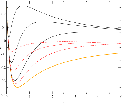
Figure 2: Hubble parameter $l=\dot{\lambda}$ as a function of cosmic time. The plotted curves represent solutions of the equations of motion with parameters $c$ and $\gamma$ chosen in the same manner as in Fig. 1.

As one can immediately see from the numerical solutions studied the efficiency parameter $c$ only qualitatively influences the very early dynamics of the equations of motion. In general, as it grows the maximum contraction rate decrease for any value of $\gamma$ (see Fig. 2) and if it is sufficiently large the universe could never enter a phase of contraction.

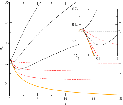
Figure 3: Scale factor as a function of cosmic time. The plotted curves represent solutions of the equations of motion with parameters $c$ and $\gamma$ chosen in the same manner as in Fig. 1.

As expected from our previous qualitative analysis the very late-time cosmological dynamics of this model is mostly independent of the parameters which characterises the decay of winding modes. In fact, the scale factor very soon behaves like,

$$\mathrm{e}^{\lambda}\sim t^{2\gamma/(1+3\gamma^{2})},$$ (27)

which corresponds to a radiation-dominated universe for $\gamma=1/3$ and to a flat static universe for $\gamma=0$. It is interesting to note that the above expansion law only coincides with that of the standard cosmological scenario for $\gamma=1/3$. This is because as the winding modes self-annihilate all trajectories approach asymptotically the line $l=-f/3$ where $\dot{\phi}\sim 0$ and $\ddot{\phi}\sim 0$. Thus, the original dilaton freezes dynamically without the need of introducing a dilaton potential and a standard expansion law is recovered before reaching the point $(f,l)=(0,0)$. This is not the case if $\gamma\neq 1/3$.

With $\gamma=0$ and for any reasonable value of the efficiency parameter $c$ we find that the universe always enters a phase of contraction after a very short period of time and never re-expands despite the self-annihilation of winding modes (see Figs. 1 and 2). Thus if the winding modes decay into static loops the spatial dimensions can never become large and the dimensionality of our spacetime cannot be explained. Apart from our previous qualitative arguments this result can also be physically understood in the following way. Eq. (19), viewed as an equation for $\lambda$, is equivalent to an equation for a damped point particle moving in an an effective potential with the following form,

$$U_{eff}(\lambda)=\frac{\tau l_{c}}{6}\mathrm{e}^{\varphi}\left[N_{w}(t)\,\mathrm{e}^{\lambda}+N_{l}(t)\,\mathrm{e}^{-3\gamma\lambda}\right].$$ (28)

In the particular case in which $\gamma=0$, the second term is no longer a function of $\lambda$ and it can be merely interpreted as a time modulation of the potential origin. For such a potential, a universe that starts expanding will reach a maximum size and, at some point, it might enter a contraction phase from which it will not be able to escape. As we have seen numerically the effect of the modulating factor $\exp(\varphi)$, which is always a decreasing function of time, is not relevant for this argument to hold. This picture changes drastically at late times if $\gamma>0$ (See Figs. 2 and 3 for the case $\gamma=1/3$). Now the second term in the effective potential $U_{eff}$ comes to dominate the dynamics as the number of winding modes $N_{w}$ goes to zero and $N_{l}$ grows. Thus, if a universe that started in a expanding phase passes through a stage of contraction it will inevitably go back to a new period of expansion. As a conclusion, we have given analytical and numerical evidences to the fact that, in contrast to the numerical results of Brandenberger et al. (2002), re-expansion in the cosmological evolution of the universe is only possible if the small loops produced do not behave like ordinary static matter.

In Fig. 4 we show the profiles of all the energy components for $\gamma=0$ and $\gamma=1/3$. In both cases, the energy of winding modes goes to zero very rapidly and, consequently, the energy of small loops tracks the total energy of the universe during most of the time evolution. One can see, in general, that the small loop energy very soon evolves as,

$$E_{l}=\tilde{E}_{l}\mathrm{e}^{-3\gamma\lambda},$$ (29)

where $\tilde{E}_{l}$ is a constant which depends on the parameters of the decay process. For $\gamma=0$ that means that the total energy reaches a constant value. We have checked numerically that the asymptotic value of this constant grows with an increasing efficiency parameter $c$. In ordinary Einstein theory a constant energy would have meant a matter-like dominated expansion of the universe. However, in our brane gas model, the effect of the dilaton coupling drives the universe through an ever contracting phase. On the other hand, for $\gamma=1/3$ we have a radiation-dominated like cosmological expansion for the universe. In this particular case the total energy decreases with time more rapidly the bigger is the parameter $c$. This is mainly due to the fact that the expansion goes faster if $c$ is larger.

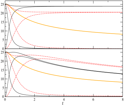
Figure 4: Energy profiles for $\gamma=0$ (top) and $\gamma=1/3$ (bottom). In both plots the dark lines correspond to $c=1.0$, the light dashed lines to $c=0.1$, and the light continuous line to $c=0$, that is, the case without winding mode decay (Recall that in this particular case $E_{l}=0$ and then the total energy is equal to $E_{w}$). The curves that asymptotically approach the zero axis represent the energy of winding modes and the curves starting at zero the energy of the loops produced. The curves tracked at late times by the loop energy is the total energy of the system $E_{l}+E_{w}$.

III.2.3 Loitering and the brane problem

The hierarchical picture of Dp-brane decay explains the actual dimensionality of spacetime though it leads to a variant of the domain wall problem in cosmology. A solution to this problem is to invoke a stage of cosmic inflation before the branes can dominate the energy density of the universe. An alternative proposed in Alexander et al. (2000), and further developed in Brandenberger et al. (2002), was to advocate a late phase of loitering in the universe. This is a stage in which the universe halts and its spatial extend $R$ could become much smaller than the Hubble horizon $d_{H}\sim l^{-1}$, that is a period in which $Rl\ll 1$.

We have checked numerically that a sufficiently long period in which this condition holds is quite natural in BGC, see Figs. 2 and 3. At early times and as long as the efficiency parameter $c$ is not too large one can assure that the Hubble horizon always becomes extremely large allowing the whole universe to be in causal contact. However, it is not hard to show that at late times one has,

$$Rl\rightarrow\left\{\begin{array}[]{ll}0&\textrm{\,\,\, for }\gamma=0,\\ t^{-1/2}&\textrm{\,\,\, for }\gamma=\frac{1}{3},\end{array}\right.$$ (30)

and then, even if the early period of loitering is not long enough the Hubble horizon always becomes larger than the spatial extend of the universe and the brane problem can be solved.

III.2.4 Scaling

An important characteristic of the evolution of a self-interacting network of strings in a expanding universe is that it reaches a stage in which its characteristic length remains constant with respect to the size of the Hubble horizon $d_{H}$ Bennett (1986b); Bennett and Bouchet (1988, 1989, 1990). An interesting question that we can answer with our analysis is whether this scaling regime is also reached when the cosmological dynamics is driven by the effects of a dilaton field.

When the evolution of the string network is assumed not to affect the standard (say, radiation- or matter-dominated) expansion of the universe, it makes no difference to talk about scaling with respect to the Hubble horizon or to the cosmic time because they are always proportional $d_{H}\sim l^{-1}\sim t$. However, when the back reaction on the dynamics of the gravitational background is taking into account the distinction between these two quantities become important because, as it happens in our problem, $d_{H}$ could become extremely large at some finite time ($l\rightarrow 0$).

To study the scaling properties of string configurations it is usually convenient to introduce a dimensionless parameter $\zeta(t)=t/L_{w}(t)$ measuring how far is the system from a scaling behaviour relative to cosmic time. The scaling regime is reached if $\zeta(t)$ relaxes to a constant value $\zeta_{\ast}$. In this situation, the decay of the number of winding modes can be expressed as,

$$N_{w}=\zeta^{2}_{\ast}\left(\frac{l_{c}}{t}\right)^{2}\mathrm{e}^{2\lambda}\sim\left\{\begin{array}[]{ll}t^{-2}&\textrm{\,\,\, for }\gamma=0,\\ t^{-1}&\textrm{\,\,\, for }\gamma=\frac{1}{3}.\end{array}\right.$$ (31)

which yields an energy density of winding modes that decrease with time independently of the equation of state of the loops created,

$$\rho_{w}=\zeta^{2}_{\ast}\left(\frac{\tau}{t^{2}}\right).$$ (32)

By substituting Eq. (31) into the dynamical equation for $N_{w}$ given in (12), it can be seen that the parameters of a scaling solution must obey the following condition,

$$c=\frac{2(1-2\gamma+3\gamma^{2})}{1+3\gamma^{2}}\zeta^{-2}_{\ast}=\left\{\begin{array}[]{ll}2\zeta^{-2}_{\ast}&\textrm{\,\,\, for }\gamma=0,\\ \zeta^{-2}_{\ast}&\textrm{\,\,\, for }\gamma=\frac{1}{3}.\end{array}\right.$$ (33)

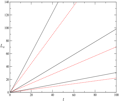
Figure 5: Characteristic length of the winding mode network as a function of cosmic time. This graph shows the scaling behaviour of the decay of winding modes. The plotted curves represent solutions of the equations of motion with parameters $c$ and $\gamma$ chosen in the same manner as in Fig. 1.

Table 1: Slopes, $\zeta^{-1}_{\ast}$, of the characteristic length $L_{w}(t)$ plotted in Fig. 5. We have also tabulated $\zeta^{-2}_{\ast}$ for an easy check of the condition (33).

	$\gamma=0$missing		$\gamma=1/3$missing
	$\zeta^{-1}_{\ast}$missing	$\zeta^{-2}_{\ast}$missing	$\zeta^{-1}_{\ast}$missing	$\zeta^{-2}_{\ast}$missing
$c=0.1$	0.2234500	0.0499299	0.3136377	0.0983686
$c=1.0$	0.7069920	0.4998377	0.9945297	0.9890893
$c=10$	2.2359990	4.9996915	3.1567680	9.9651842

From our numerical simulations (see Fig. 5 and Table 1) we readily observed that $\zeta(t)$ relaxes very rapidly to a constant value and, then, $L_{w}$ scales with cosmic time $t$. Moreover, apart from numerical errors, our solutions also satisfy the above scaling relation with high accuracy. To check if the system also scales with the cosmological horizon one has to recall from the previous subsection that at very early times the size of the horizon can become extremely large but soon after the winding modes have disappeared it behaves as,

$$d_{H}\sim l^{-1}\sim\frac{1+3\gamma^{2}}{2\gamma}\,t.$$ (34)

Consequently, this means that for values of $\gamma>0$ the characteristic length of the network configuration will inevitably evolve to a scale comparable to the cosmological horizon. On the contrary, if $\gamma=0$, the string network can never scale with $d_{H}$ despite it does with cosmic time. This is closely related with the fact that, in this case, the universe reaches an indefinitely large period of loitering.

We would also like to mention that we have check numerically that these scaling properties do not change significantly if we take the typical size of the loops produced to scale with the characteristic length of the winding mode network, $L_{l}\sim L_{w}$, instead of taking a size that scales with cosmic time.

III.2.5 A gas of non-static branes

The equation of state for the winding modes we have considered in our previous analysis, Eq.  (4), corresponds to a gas of non-relativistic branes. Let us briefly comment how we expect the cosmological dynamics will be affected if the early evolution is dominated by a gas of non-static branes. The generalised equation of state is characterised by a new parameter $\gamma_{p}$ given by (see for instance Boehm and Brandenberger (2002); Vilenkin and Shellard (1994)),

$$\gamma_{p}=\left(\frac{p+1}{D}\langle v^{2}\rangle-\frac{p}{D}\right),$$ (35)

where $\langle v^{2}\rangle$ is the average of the squared velocity at each point of a brane. For $\langle v^{2}\rangle\rightarrow 1$ the gas of branes behaves as a gas of relativistic particles whereas the non-relativistic or static limit corresponds to $\langle v^{2}\rangle\rightarrow 0$. In the case of winding modes with $p=1$ in $D=3$ spatial dimensions we have a modified evolution equation for the Hubble parameter $l$ depending on this new characteristic velocity of the brane gas,

$$\dot{l}=fl-\frac{1}{6}\,\mathrm{e}^{\varphi}\left[(1-2\langle v^{2}\rangle)E_{w}-3\gamma E_{l}\right].$$ (36)

The first point to stress is that the very late-time cosmological evolution will not be qualitatively altered and the special lines $l=-\gamma f$ will still continue to be solutions of the equations of motion and attractors of the rest of trajectories close to the critical point $(0,0)$ in the phase space spanned by $(f,l)$. On the other hand, the rules for crossing these special lines away from the origin are significantly modified and this has interesting dynamical consequences. Eq (26) now reads,

$$\ddot{\Phi}=-\frac{\mathrm{e}^{\varphi}}{6}\left(1+3\gamma-2\langle v^{2}\rangle\right)E_{w},$$ (37)

and then, it is very easy to see, following the same argumentation of previous sections, that now crossings from values of $f$ and $l$ with $l+\gamma f<0$ to values with $l+\gamma f>0$ will be allowed if,

$$\langle v^{2}\rangle>\frac{3\gamma+1}{2}.$$ (38)

For $\gamma=0$ this means that the average velocity $\langle v^{2}\rangle$ has to be greater than $1/2$. However, if this condition is satisfied the Hubble parameter $l$ cannot have a turning point with $fl>0$, that is with a negative value of $l$ (contracting phase). Thus, contrary to what happens when the branes are static, a universe that was initially expanding will ever stay expanding. But more interesting, if the universe started in a contracting phase it can now, for moderate values of the efficiency parameter, enter a stage of expansion before asymptotically reaching $(f,l)=(0,0)$. This stage of late expansion when the branes of the gas are not static makes the case in which the loops produced behave like ordinary matter to regain a phenomenological interest because this solves the obstruction discussed in previous sections to explain the dimensionality of our spacetime.

One might also ask whether it is still possible to ensure the small string coupling approximation dynamically for solutions with initial conditions satisfying the inequality $l<-f/3$ as for the $\langle v^{2}\rangle=0$ case since now crossings of the special lines are in principle allowed. Fortunately, this criterion is still valid because the line $l+f/3=0$ cannot be cross from the region with $l+f/3<0$ (decreasing dilaton) to the region $l+f/3>0$ (growing dilaton) unless the brane gas has an exotic characteristic velocity which exceeds the velocity of light, $\langle v^{2}\rangle>1$.

With respect to the scaling properties of the winding mode decay, we do not expect significative modifications relative to the picture already outline for a gas of static branes.

IV Conclusions

In this work we have elaborated a detailed discussion of the late-time behaviour of brane gas cosmologies which have served to clarify and better understand some relevant issues of their dynamics.

As a conclusion we have found that in order to obtain a phenomenologically interesting cosmological evolution the loops produced without winding number have to behave as a gas with an equation of state characterised by a parameter satisfying $0<\gamma\leq 1/3$. Otherwise, the string coupling becomes large and the low-energy effective description fails (for $\gamma>1/3$), or the spatial dimensions do not grow and the dimensionality of our present universe cannot be explained (for $\gamma\leq 0$). One would expect that the first difficulty could be alleviated simply by introducing higher-order quantum corrections. As we have seen, one can avoid the second obstacle by considering the dynamics of a gas with non-static branes. An alternative to obtain a late phase of expansion for $\gamma\leq 0$ is to include the effects of an axion or a moduli field. The problem with this option is that the dilaton evolves in general towards regions in phase space with a strong string coupling Foffa et al. (1999); Tsujikawa (2003). In our analysis we have assumed for simplicity that the characteristic velocity of the brane gas $\langle v^{2}\rangle$ is constant. An interesting open question would be to find out whether the more realistic situation in which this velocity also varies with cosmic time could reveal new cosmological features.

On the other hand, we have also confirmed that an early phase of loitering appears generically in brane gas scenarios if the efficiency parameter of the decay of winding modes takes moderate values. The existence of this phase in which the Hubble horizon becomes larger than the spatial extend of the universe offers a simple resolution to the brane problem as suggested in Alexander et al. (2000). In fact, the final fate of the universe in these type of cosmologies is always that of a loitering universe because the Hubble parameter goes to zero very slowly at late times. Thus, even for those cases in which the early period of loitering does not occur, or is not long enough to provide a causal microphysical explanation for a complete disappearance of branes, the brane problem can also be solved.

Finally, we have investigated whether the evolution of a network of winding modes driven by the dynamics of a dilaton field reaches a stage in which its characteristic length remains constant with respect to the size of the Hubble horizon $d_{H}$ as for ordinary cosmic strings in a expanding universe. We have shown that for values of $\gamma>0$ the characteristic length of the network will always scale with the cosmological horizon. However, for the particular case in which $\gamma=0$, the network never scales with $d_{H}$ despite it does with cosmic time. This is closely related with the fact that, in this case, the universe reaches an indefinitely large period of loitering.