Tachyon kinks on non BPS D-branes

Abstract

We consider solitonic solutions of the DBI tachyon effective action for a non-BPS brane. When wrapped on a circle, these solutions are regular and have a finite energy. We show that in the decompactified limit, these solitons give Sen’s infinitely thin finite energy kink — interpreted as a BPS brane — provided that some conditions on the potential hold. In particular, if for large $T$ the potential is exponential, $V=e^{-T^{a}}$, then Sen’s solution is only found for $a<1$. For power-law potentials $V=1/T^{b}$, one must have $b>1$. If these conditions are not satisfied, we show that the lowest energy configuration is the unstable tachyon vacuum with no kinks. We examine the stability of the solitons and the spectrum of small perturbations.

1 Introduction

In addition to the stable and charged BPS D-branes [1], type II superstrings contain unstable and uncharged non-supersymmetric D-branes [2]. The instability of these non-BPS branes is signalled by the presence of a tachyon on their worldvolume. The decay of non-BPS branes is described by the dynamics of this tachyon. Sen has also proposed the remarkable fact that the BPS branes can also be viewed as tachyon kinks on the non-BPS branes with one dimension higher [3]. Different approaches [6, 7, 8, 9, 10, 11, 12, 13, 14] converged to the following Dirac-Born-Infeld (DBI) effective action describing the dynamics of the tachyon field $T$:

$$S=-\int d^{p}x\,dt\,V(T)\sqrt{\left(1+\partial_{\mu}T\partial_{\nu}T\eta^{\mu\nu}\right)}.$$ (1.1)

Here $V(T)$ is the tachyon potential which is even and vanishes at infinity where it reaches its minimum. Near the global maximum at $T=0$, $V(T)={\cal T}_{p}(1-\beta^{2}T^{2}/2)+\dots$ where ${\cal T}_{p}$ is the tension of the non-BPS $p$-brane and the potenial encodes the mass of the tachyon near the perturbative vacuum $T=0$. Finally $\eta^{\mu\nu}=(-1,+1,\ldots,+1)$ is the $p+1$ Minkowski metric.

Finite energy solitons obtained from the DBI action and depending on one spatial coordinate (kinks) are singular [15, 16, 17]. The goal of the present paper is to construct these kinks as limits of regular solitons by compactifying the spatial coordinate and looking for conditions on the potential which guarantee the existence of the decompactified limit. We shall show that the existence of this limit implies two new conditions on the potential $V(T)$ as $T\rightarrow\infty$: i) that $|V^{\prime}|/V$ must tend to zero, and ii) that $|V^{\prime}|/V^{2}$ must tend to infinity.

The action (1.1) is supposed to be valid for large $T$ and small higher order derivatives of $T$, and this is compatible with the limit we are considering. Our results, together with the ones coming from time dependent solutions [11, 13], boundary string field theory [18] and perturbative amplitude calculations [14], give constraints on the potential of the tachyon in different regimes and hopefully may help to determine an effective action capturing a large domain of validity. On the other hand, if the potential is determined by other means and found not to satisfy the conditions i) and ii) above (as is the case for a number of potentials studied in the literature), then we would conclude that the DBI has no stable kink solution.

The plan of this paper is as follows. In Section 2 we revisit Derrick’s theorem which gives necessary conditions for the existence of finite energy solitons for actions of the form (1.1). Within this framework we show how the infinitly thin kink may appear. In Section 3, we compactify one spatial coordinate on a circle of radius $R$ in order to get regular kinks. In fact, we obtain regular solitons describing $n$ pairs of kinks and anti-kinks. This is to be expected since the net RR charge is zero in a compact space. The kink and anti-kink are separated by a distance $2\zeta=2\pi R/2n$ and the energy of the configuration has the form $2n{\cal E}(\zeta)$. The decompactified limit corresponds to $\zeta\rightarrow\infty$ with $\cal E$ finite in the limit. In Section 3.1 we determine the conditions on the potential, stated above, for which this limit exists. We also give some examples; in particular, for exponentially decaying potentials of the form $e^{-T^{a}}$ we show that the conditions are satisfied if and only if $a<1$. For power-law decay, $V=T^{-b}$, they are satisfied if and only if $b>1$. In Section 4 we examine the stability of the solitons and show that the unstable fluctuations disappear in the decompactified limit whenever this limit is well defined. Finally conclusions are presented in Section 5.

2 Solitons and Derrick’s theorem

We aim to search for solitonic or kink-like solutions of (1.1). These kink solutions should represent the stable BPS $p-1$ branes into which the non-BPS $p$-brane decays. Before doing this explicitly, it is worthwhile recalling Derrick’s theorem [19]: in the case of the usual Klein-Gordon action for scalar fields, it tells us that finite energy static solitonic solutions on an infinite space are only possible in (1+1)-dimensions. In this section we will draw similar conclusions starting from (1.1).

In fact, to make contact with the literature, we will initially consider a slightly more general action:

$$S=-\int d^{p}x\,dt\,V(T)\left(1+\partial_{\mu}T\partial_{\nu}T\eta^{\mu\nu}\right)^{q},$$ (2.1)

where the real scalar field $T$ is dimensionless (we set $\alpha^{\prime}=1$ throughout). For $q=1/2$ this is just (1.1). The case $q=1$ has also been proposed as an effective tachyon action (see, for instance, [17]), whose kinks were studied in [20]. We will recover some properties of these kinks using Derrick’s theorem.

To recall Derrick’s theorem, consider first a canonical scalar field $\phi(\vec{x},t)$ with action

$$S_{\rm KG}=\int d^{p}x\,dt\left(-\frac{1}{2}\partial_{\mu}{\bf\phi}\partial^{\mu}{\bf\phi}-W(\phi)\right)$$ (2.2)

where the $p$ spatial directions are infinite, and the potential $W(\phi)$ is non-negative vanishing only at its absolute minima. Let $\phi_{1}(x)$ be a static solution of the equations of motion, and hence an extremum, $\delta E=0$, of the finite static energy functional

$$E[\phi]=\int d^{p}x\left(\frac{1}{2}\partial_{i}{\phi}\partial^{i}{\phi}+W(\phi)\right)\qquad(i=1,\ldots,p).$$ (2.3)

Now consider a one parameter family of solutions $\phi_{\lambda}(x)=\phi_{1}(\lambda x)$. Since $\phi_{1}(x)$ is an extremum of $E$, then $\left.\frac{d}{d\lambda}E[\phi_{\lambda}]\right|_{\lambda=1}=0$ leading to

$$0=\int d^{p}x\left(p\,W(\phi)+(p-2)\frac{1}{2}\partial_{i}{\phi}\partial^{i}{\phi}\right).$$ (2.4)

Thus when $p\geq 2$, only the vacuum solution ($W(\phi)=0$, $\phi=$const) is allowed. Only if $p=1$ may non-trivial ${\vec{x}}$-dependent solutions exist.

We now carry out a similar analysis for the tachyon action (2.1). The static energy functional is

$$E[T]=\int d^{p}xV(T)\left(1+\partial_{i}T\,\partial^{i}T\right)^{q},$$ (2.5)

and proceeding as above leads to the constraint

$$0=\int d^{p}xV(T)\left(1+\partial_{i}T\,\partial^{i}T\right)^{q-1}\left[p+(p-2q)\partial_{i}T\,\partial^{i}T\right].$$ (2.6)

Notice that, as opposed to (2.4), the potential $V(T)$ appears as an overall multiplicative factor.

When $q=1$ the term in square brackets in (2.6) only vanishes and gives non-trivial solutions if $p=1$, i.e. in (1+1) dimensions. In this case, (2.6) imposes that

$$T^{\prime 2}=1\qquad\Longrightarrow\qquad T=\pm x.$$ (2.7)

(From now on, the kink will be taken to be centered about $x=0$: $T(0)=0$.) This kink/anti-kink solution has been discussed elsewhere [20] and it is easy to verify that $T=\pm x$ is indeed a solution of the equations of motion. Such solutions are topological, interpolating from one vacuum to another, and from (2.5) their energy (or tension ${\cal T}_{p-1}$) is given by

$$E={\cal T}_{p-1}=2\int_{-\infty}^{\infty}V(x)dx$$

which, if $V$ decays sufficiently fast at infinity, is finite. Notice that from the properties of $V(T)$, the energy density of the field is localised around $x=0$ and the width of the resulting kink (or BPS brane) is determined by the parameters in $V(T)$. These parameters must be tuned such that ${\cal T}_{p-1}$ takes the correct value. Furthermore, by considering small perturbations about the solution $T(x,t)=\pm x+f(x,t)$ and linearising the equations of motion, it is possible to show that if $E$ is finite, solutions (2.7) are stable against small perturbations.

When $q=1/2$, the case we focus on here, the square bracket in (2.6) is $p+(p-1)\partial_{i}T\partial^{i}T$ which can never vanish for $p\geq 1$. Thus no finite energy static solutions seem to be permitted. However, there is formally a way around this: when $p=1$ (2.6) becomes

$$0=\int d^{p}x\frac{V(T)}{\sqrt{1+T^{\prime 2}}}$$ (2.8)

which can vanish if

$$T^{\prime}\rightarrow\pm\infty\qquad{\rm or}\qquad T\rightarrow\infty$$

with $E[T]$ remaining finite. Let us suppose that the equations of motion admit a solution with $T^{\prime}\rightarrow\pm\infty$ describing a single kink (below we will find the conditions on $V(T)$ such that this is the case),

$$T(x)=\lim_{C\rightarrow 0}\frac{x}{C}=\left\{\begin{array}[]{cl}\infty&x>0\\ 0&x=0.\\ -\infty&x<0\end{array}\right.$$ (2.9)

This is a typical case of the solutions discussed by Sen [15]: it describes an infinitely thin topological kink interpolating between the two vacuua. Notice that $V=0$ everywhere apart from when $T=0=x$. Substitution of (2.9) into the energy functional (2.5) (taking carefully the $C\rightarrow 0$ limit) gives the the energy of this singular solution to be

$$E_{\rm Sen}=\int_{-\infty}^{\infty}V(x)dx.$$ (2.10)

Sen has argued that such singular kinks are stable, as the BPS brane should be, and furthermore that their effective action is exactly the required DBI action [15]. Hence such solutions are of great interest, and would suggest that BPS branes are infinitely thin. Once again the parameters of $V(T)$ should be tuned such that $E_{\rm Sen}={\cal T}_{p-1}$.

The question we ask in this paper is the following: do the equations of motion for $T$ always admit a single infinitely thin singular kink solution with energy given by (2.10)? As we will show, the answer depends sensitively on the shape of the tachyon potential $V(T)$ for large $T$. For instance, for $V(T)\sim\exp(-T^{a})$ with $a\geq 1$, this solution does not exist. Our approach will be to try to find a regularised kink solutions from which Sen’s singular limit can then be approached. This can be done through compactification.

3 Regularised kinks and examples

We are looking for static kink-like solutions in which $T$ has a non-trivial dependence only on one spatial coordinate; $T=T(x)$. Let as assume that the kink is centered at the origin,

$$T(0)=0.$$ (3.1)

The equations of motion coming from (2.1) with $q=1/2$ have a first integral,

$${V(T)\over\sqrt{1+(T^{\prime})^{2}}}=V_{0},$$ (3.2)

where $V_{0}\geq 0$ is a constant. The energy of this solution is given by

$$E=\int dxV(T)\sqrt{1+(T^{\prime})^{2}}=\frac{1}{V_{0}}\int dxV^{2}(T).$$ (3.3)

Since $T^{\prime 2}$ is positive, solutions of equation (3.2) exist in the region

$$V(T)\geq V_{0}\qquad({\rm soliton\;solution)}.$$ (3.4)

Furthermore, the solutions $T(x)$ are periodic (see figure 1) with a $V_{0}$-dependent amplitude which, from (3.2), diverges as $V_{0}\rightarrow 0$. Note that within one period there must be both a kink and an anti-kink (corresponding to the two points for which $T(x)=0$), as can clearly be seen in figure 1. Also, the energy density of the kinks becomes more and more localised as $V_{0}\rightarrow 0$. Below we will study in detail the dependence of both the period and $E$ on $V_{0}$.

         

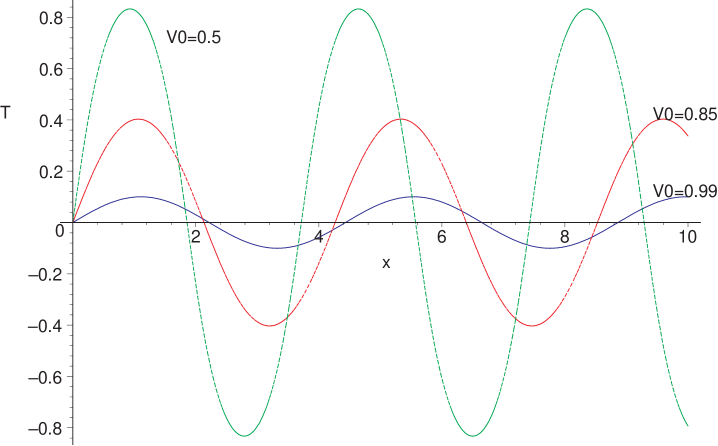
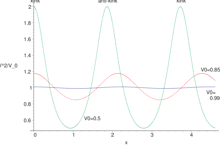
Figure 1: LH panel: The solution $T(x)$ of equation (3.2) for the potential $V=e^{-T^{2}}$. As discussed in the text, the solutions are periodic and their amplitude increases as $V_{0}$ decreases: the 3 curves correspond to $V_{0}=0.5$ (green curve), $V_{0}=0.85$ (red curve), and $V_{0}=0.99$ (blue curve). Note, as will be discussed later, that the wavelength of the solutions decreases as $V_{0}$ decreases. RH panel: the energy density $V^{2}/V_{0}$ corresponding to the 3 curves in the LH panel. The kinks and anti-kinks are labeled. Note that as $V_{0}$ decreases the energy density in the kinks and anti-kinks have more localised energy density.

In order for $E$ to be finite, one must have $|T|\rightarrow\infty$ as ${|x|\rightarrow\infty}$. This immediately implies from (3.2) that $V_{0}=0$ — a topological kink. Sen’s solution [15] (2.9) is such a singular solution in which $T$ vanishes for only one value of $x$: in other words Sen’s solution is periodic with a divergent wavelength. Furthermore in that case $E=2E_{\rm Sen}$.

We would like to approach the singular ($V_{0}\rightarrow 0$) kink(s) as the limit of regular solutions with $V_{0}\neq 0$. In order to get regular and finite energy solutions we shall suppose that $x$ is a compact direction of length $2\pi R$, so that $V_{0}$ can now be non-zero. Our aim is to see whether the limit $R\rightarrow\infty$ with $E$ being finite exists. Note that if this limit exists we expect to get twice (2.10) as the energy of the resulting solution. We can see this from several points of view: BPS branes have a RR charge and on a circle the sum of the charges must vanish so all we can get are pairs of branes and anti-branes. Sen’s solution corresponds to the brane infinitely distant from the anti-brane. Alternatively note that on a circle the solution is periodic, so if a kink is present at the origin, where $T^{\prime}$ is positive, then necessarily an anti-kink will also be present since as $\int_{0}^{2\pi R}T^{\prime}dx=0$, $T^{\prime}$ must be negative somewhere between $0$ and $2\pi R$. So if we can regularise Sen’s solution by compactifying the $x$ coordinate, the limiting energy is expected to be twice the value (2.10). Half of this corresponds to the anti-kink which is sent to infinity, so that we recover $E_{\rm Sen}$ for the remaining kink.

Since the wavelength of the kink solutions is $V_{0}$ dependent, not all values of $V_{0}$ will be permitted for a given radius $R$. The dependence of $V_{0}$ on $R$ can be determined as follows: the period of the solutions of equation (3.2) is $4\zeta$ where

$$\zeta(V_{0})=\int_{0}^{T_{0}}{dT\over{\sqrt{\left(V\over V_{0}\right)^{2}-1}}},$$ (3.5)

and $T_{0}$ is defined by $V(T_{0})=V_{0}$. The radius is thus given by

$$2\pi R=4n\zeta,$$ (3.6)

where $n=1,2,\dots$. The separation between the brane and the anti-brane is $2\zeta$. The $V_{0}$-dependent energy of this solution can be written as

$$E(V_{0}) = 4n\int_{0}^{\zeta}dx{V^{2}(T)\over V_{0}}=4n\int_{0}^{T_{0}}dT{V\over{\sqrt{1-\left(V_{0}\over V\right)^{2}}}}$$ (3.7)

$$\equiv 4n{\cal{E}}(V_{0}).$$ (3.8)

To summarise, $V_{0}$ is implicitly determined by equation (3.6) in terms of an integer $n$ and the radius $R$. The energy of the solution depends on $R$ and on $n$. Note that this dependence is complicated by the presence of $V_{0}$ in (3.7).

The limit when $V_{0}\rightarrow 0$ or equivalently $T_{0}\rightarrow\infty$ is not transparent for $\zeta$ and $\cal E$. There is, however, a combination of both for which the limit is known: consider

$$\Delta(V_{0})\equiv{\cal E}-\zeta V_{0}=\int_{0}^{T_{0}}dT\sqrt{(V^{2}-V_{0}^{2})}.$$ (3.9)

Then as $V_{0}$ goes to zero

$$\Delta(V_{0})\rightarrow\int_{0}^{\infty}dT\;V(T),$$ (3.10)

which is exactly $E_{\rm Sen}/2$.

Let us examine the limit where the radius goes to infinity. There are three possibilities depending on the behaviour of $\zeta(V_{0})$ as $V_{0}\rightarrow 0$:

1. $\zeta\rightarrow\infty$ as ${V_{0}\rightarrow 0}$. The kink anti-kink separation tends to infinity, and as $R\rightarrow\infty$, equation (3.6) can be satisfied with $n=1$ — a single kink. From equation (3.10) we see that the energy goes to $2\int_{-\infty}^{\infty}V(T)dT$ if and only if $\zeta V_{0}\rightarrow 0$.

2. $\zeta\rightarrow$ const $\neq 0$ as ${V_{0}\rightarrow 0}$. Now the kink anti-kink distance tends to a constant (independently of $R$) and one can never get an isolated kink. As $R\rightarrow\infty$, equation (3.6) can only be satisfied if $n\rightarrow\infty$. In this case (3.7) shows that that are no finite energy solutions in the decompactified limit. For a given finite $R$, $E$ is however finite.

3. $\zeta\rightarrow 0$ as $V_{0}\rightarrow 0$. For a fixed $R$, the limit $V_{0}\rightarrow 0$ now leads to an array of infinitely many singular kinks and anti-kinks (since their separation is $2\zeta(0)$). From (3.8) the energy (even for finite $R$) is infinite. This is a rather problematic (and not very meaningful) limit, but we will see that this behaviour occurs for many potentials considered in the literature; for example $V(T)=ve^{-T^{2}}$.

As we shall show in the next subsection, the behaviour of $\zeta(V_{0})$ as $V_{0}\rightarrow 0$ depends critically on the form $V(T)$ for large $T$. Before doing that, we present a very simple example of case (2) above, and hence a potential for which Sen’s solution can not be recovered. Let

$$V(T)=\frac{v}{\cosh\beta T}.$$ (3.11)

(This potential has also been analysed elsewhere [21] and motivated from string theory calculations in [13].) On substitution into (3.2) it is straightforward to solve for $T(x)$: one finds

$$T(x)={\rm arc}\sinh\left[\frac{1}{\beta}\left(\frac{v^{2}}{V_{0}^{2}}-1\right)^{1/2}\sin(\beta x)\right],$$ (3.12)

which is indeed periodic with a divergent amplitude in the singular $V_{0}\rightarrow 0$. Notice, however, that the period is independent of $V_{0}$:

$$\zeta(V_{0})=\frac{\pi}{2\beta}\;,\qquad\forall\;V_{0}.$$ (3.13)

Thus as $V_{0}\rightarrow 0$, $\zeta$ remains constant leading to an array of localised kink-anti-kink pairs. Let us now compactify on the circle of radius $R=4n\zeta/2\pi=n\pi/\beta$, where $n=1,2,\ldots$ counts the number of kinks. (This limiting potential has the unusual feature that for a given $R$, $V_{0}$ need not take discrete values: all values between $0$ and $v$ are allowed.) Using (3.12) the energy (3.7) of the solution is easily obtained, after a contour integration, to be

$$E=\frac{4n}{V_{0}}\int_{0}^{\frac{\pi}{2\beta}}\frac{v^{2}}{\cosh^{2}(\beta T(x))}dx=\frac{2\pi v}{\beta}n=2\pi Rv$$ (3.14)

i.e. independent of $V_{0}$. Thus each solution is equally energetic. In the limit $R\rightarrow\infty$ the energy diverges and is clearly not given by (2.10).

In the next subsection we determine the conditions which $V$ must satisfy so that in the decompactified limit with a finite energy, $\zeta$ diverges.

3.1 Solitonic solutions on the circle

From the discussion in the previous section, the dependence of $\zeta$ on $V_{0}$ when $V_{0}$ is small is crucial. In order to analyse this dependence let us parametrise the general potential $V(T)$ by

$$V(T)=\frac{v}{\cosh f(T)}$$ (3.15)

where $f(0)=0$. Then, on letting

$$u=\frac{\sinh f(T)}{\sinh f(T_{0})},$$ (3.16)

the period $\zeta(V_{0})$ in (3.5) becomes

$$\zeta(V_{0})=\int_{0}^{1}du\frac{1}{\sqrt{1-u^{2}}}\frac{1}{\left|\frac{df(T(u,V_{0}))}{dT}\right|}.$$ (3.17)

Notice immediately that if $f(T)=T$ (i.e. the potential discussed in the previous section), we recover the constant $\zeta$. Clearly the dependence of $\zeta(V_{0})$ is determined by $f^{\prime}$. The $V_{0}$-dependence of $f^{\prime}(T(u,V_{0}))$ is through the combination $u\sqrt{(v/V_{0})^{2}-1}$. Thus from (3.17), the behaviour of $\zeta(V_{0}\rightarrow 0)$ depends on $f^{\prime}(T\rightarrow\infty)$. Since $|f^{\prime}|\sim|V^{\prime}|/V$ it follows that

$$\zeta(V_{0})\rightarrow\frac{\pi}{2}\left.\frac{V}{|V^{\prime}|}\right|_{T_{0}}\qquad(V_{0}\rightarrow 0\;,\;T_{0}\rightarrow\infty).$$ (3.18)

Since the potential is assumed positive let us write it in the form $V=e^{-\sigma(T)}$ then the condition for $\zeta$ to diverge in the limit $T_{0}\rightarrow\infty$ reads

$$\lim_{T\rightarrow\infty}\sigma^{\prime}(T)=0.$$ (3.19)

This is one of our main results. This condition is clearly not satisfied for the $e^{-aT^{2}}$ potential. In fact this potential gives rise to $\zeta$ which vanishes in the $V_{0}\rightarrow 0$ limit: an example of case 3 discussed in the previous section. Thus for exponential potentials, in the limit $V_{0}\rightarrow 0$,

$$V(T\rightarrow\infty)\sim\exp(-T^{a})\qquad\Rightarrow\qquad\left\{\begin{array}[]{ll}a<1,&\zeta\rightarrow\infty\\ a>1,&\zeta\rightarrow 0\\ a=1,&\zeta\rightarrow K\neq 0\end{array}\right.$$ (3.20)

For power-law potentials, again in the limit $V_{0}\rightarrow 0$:

$$V(T\rightarrow\infty)\sim\frac{1}{T^{1/\alpha}}\qquad\Rightarrow\qquad\left\{\alpha>0,\qquad\zeta\rightarrow\infty\right.$$ (3.21)

where the condition on $\alpha$ simply enforces that $V(T)$ vanishes at infinity.

Before turning to the energy, it is useful to derive two further results for the period $\zeta(V_{0})$. The first is the value of $\zeta(V_{0}=v)$. Let us suppose that $V_{0}=v-\epsilon$, ($\epsilon\ll v$), so that the tachyon oscillates around $T=0$ with a very small amplitude. Thus $V(T)=v(1-\beta^{2}T^{2}/2)+{\cal{O}}(T^{4})$ where $\beta$ is dimensionless, and the solution of (3.2) is

$$T(x)=\frac{1}{\beta^{2}}\left(1-\frac{V_{0}^{2}}{v^{2}}\right)\sin(x\beta).$$ (3.22)

Hence

$$\zeta(v)=\frac{\pi}{2\beta}\qquad{\rm and}\qquad\left.\frac{d\zeta}{dV_{0}}\right|_{V_{0}=v}=0.$$ (3.23)

Secondly, it will be useful to express $T(V)$ as an integral over $\zeta(V_{0})$. To do so, note that since

$$\int_{a}^{b}\frac{dx}{\left[(x-a)(b-x)\right]^{1/2}}=\pi$$

for arbitrary $a$ and $b>a$, equation (3.5) can be inverted to give

$$T(V)=\frac{1}{\pi}\int_{V}^{v}dx\,\frac{\zeta(x)}{(x^{2}-V^{2})^{1/2}}=\frac{1}{\pi}\int_{0}^{{\rm arc}\cosh(v/V)}d\theta\;\zeta(V\cosh\theta)$$ (3.24)

where $x=V\cosh\theta$. Thus if we specify a particular behaviour of $\zeta(x)$ we can use (3.24) to determine $T(V)$ which can then be inverted to find $V(T)$. This will be done in subsection 3.2 where it will be useful to note from (3.24) that the vanishing of the potential as $|T|\rightarrow\infty$ imposes the condition

$$\int_{0}^{v}dV_{0}\;\left(\frac{\zeta(V_{0})}{V_{0}}\right)\rightarrow\infty.$$ (3.25)

We now ask what conditions $V(T)$ must satisfy such that as $V_{0}\rightarrow 0$ and $R\rightarrow\infty$ the energy $E$ in (3.7) with $n=1$ reduces to $2E_{\rm Sen}$ in (2.10). First notice from equations (3.9), (3.10) and (3.18) that ${\cal{E}}(V_{0})$ will be finite if and only if, as $T\rightarrow\infty$,

$${|V^{\prime}|\over V^{2}}\rightarrow\infty.$$ (3.26)

This condition should be contrasted with the condition (3.18) on $\zeta$. In this case, ${\cal E}\rightarrow\int_{0}^{\infty}V(T)dT$. Thus from (3.26) we conclude that for exponential potentials

$$V(T\rightarrow\infty)\sim\exp(-T^{a})\qquad\Rightarrow\qquad{\cal{E}}\;{\rm finite}\;\forall\;a>0$$ (3.27)

whereas for power-law potentials

$$V(T\rightarrow\infty)\sim\frac{1}{T^{1/\alpha}}\qquad\Rightarrow\qquad{\cal{E}}\;{\rm finite}\;\iff\;\alpha<1.$$ (3.28)

Now, recalling that $E=4n{\cal{E}}$, we can ask whether $E$ is finite in the decompactified limit $R\rightarrow\infty$ as $V_{0}\rightarrow 0$. Combining the conditions (3.20) and (3.27) for exponential potentials gives, in these limits

$$V(T)\sim\exp(-T^{a})\;\;{\rm as}\;\;R\rightarrow\infty\;\;{\rm and}\;\;V_{0}\rightarrow 0:$$

$$\begin{array}[]{c}{\cal{E}}\rightarrow\int_{0}^{\infty}V(T)\,dT\\ \forall\;a>0\end{array}$$

(3.29)

For power-law potentials, one finds instead

$$V(T)\sim\frac{1}{T^{1/\alpha}}\;\;{\rm as}\;\;R\rightarrow\infty\;\;{\rm and}\;\;V_{0}\rightarrow 0:$$

$$\begin{array}[]{c}\zeta\rightarrow\infty\;{\rm and}\;n=1\\ \forall\;\alpha>0\end{array}$$

(3.30)

3.2 Some examples and solutions for $\zeta(V_{0})$

In this subsection we give the exact $\zeta$ behaviour (focusing mainly on the $V_{0}\rightarrow 0$ limit) for both power-law and exponential potentials.

First suppose that

$$\zeta(V_{0})\sim V_{0}^{-\alpha}.$$ (3.31)

Then (3.25) imposes that

$$\alpha>0$$ (3.32)

so that $\zeta$ always diverges in the $V_{0}\rightarrow 0$ limit. Note, however, that (3.31) cannot be valid $\forall\;V_{0}$: though it can be normalised correctly at $V_{0}=v$, its gradient will not vanish there, as required by (3.23). Hence let us first consider the large $T$ or small $V_{0}$ behaviour. What is the potential $V(T)$ corresponding to (3.31)? This can be obtained by a simple substitution into (3.24): for large $T$

$$T(V)\sim V^{-\alpha}\qquad\Longrightarrow\qquad V(T)\sim\frac{1}{T^{1/\alpha}}.$$ (3.33)

Hence we have recovered part of the results of table (3.30): for $V(T)\sim\frac{1}{T^{1/\alpha}}$, one must have $\alpha>0$ and furthermore in that case $\zeta$ diverges as $V_{0}^{-\alpha}$. Alternatively, starting from (3.33) we could have deduced (3.31) from (3.18).

Furthermore it is useful to notice from (3.17) that if

$$V(T)=\frac{v}{T^{\alpha}}\qquad({\rm i.e}\;\cosh f(T)=T^{\alpha})$$ (3.34)

then

$$\frac{d\zeta}{dV_{0}}\leq 0\qquad\forall\;V_{0}.$$ (3.35)

Thus, as an example, one could take

$$\zeta(V_{0})=\frac{\pi}{2\beta}v^{2\alpha}\frac{1}{[V_{0}(2v-V_{0})]^{\alpha}}$$ (3.36)

which satisfies all the necessary criteria for $\zeta$ (see (3.23,3.25,3.35)) and can be integrated exactly for various values of $\alpha$ (such as $\alpha=1/2,1,2$). The answer is not particularly illuminating, though a simple plot shows that it yields a potential $V(T)$ with vanishing first derivative at $T=0$ and which goes as $T^{-1/\alpha}$ for large $T$.

Secondly suppose that,

$$\zeta(V_{0})\sim\frac{1}{(-\ln(V_{0}))^{\frac{a-1}{a}}},$$ (3.37)

so that as $V_{0}\rightarrow 0$,

$$a>1\Rightarrow\zeta\rightarrow 0\,,\qquad a<1\Rightarrow\zeta\rightarrow\infty\,,\qquad a=1\Rightarrow K\neq 0.$$ (3.38)

Again, note that (3.37) cannot be valid for all $V_{0}$. Substitution of (3.37) into (3.24) shows that for large $T$,

$$T(V)\sim(-\ln V)^{1/a}\qquad\Longrightarrow\qquad V(T)\sim\exp({-T^{a}}):$$ (3.39)

(3.37) generates exponentially decaying potentials. Thus (3.38) confirms our previous results of (3.29). Finally, as above, one can deduce from (3.17) that if $f(T)=T^{a}$ then for all $V_{0}$,

$$\frac{d\zeta}{dV_{0}}\leq 0\;,\;a<1\qquad,\qquad\frac{d\zeta}{dV_{0}}\geq 0\;,\;a>1.\qquad\qquad(\forall\;V_{0})$$ (3.40)

3.3 Energy for a fixed finite $R$

Finally, in this subsection we suppose that $R$ is finite and fixed, and ask which value of $V_{0}$ is most favoured energetically. In other words, we calculate $E_{R}(V_{0})$ and ask for what value of $V_{0}$ it is minimal.

Clearly when $V_{0}=v$, $E_{R}(v)=2\pi Rv$ since the field $T$ is constant and vanishing. Furthermore we have seen in (3.14) that for the limiting potential $V=v/\cosh(\beta T)$ the energy is $V_{0}$ dependent and also given by $E_{R}(V_{0})=2\pi Rv$. In general, though, how does $E_{R}(V_{0})$ behave depending on whether $\zeta$ diverges or tends to zero as $V_{0}$ tends to zero? To see that, it will be useful to note from (3.8) and (3.9) that

$$E_{R}(V_{0})=4n{\cal{E}}=2\pi R\left[\frac{1}{\zeta(V_{0})}\int_{0}^{T_{0}}(V^{2}-V_{0}^{2})^{1/2}dT+V_{0}\right]$$ (3.41)

and hence

$$\frac{dE_{R}(V_{0})}{dV_{0}}=-2\pi R\frac{1}{\zeta^{2}}\frac{d\zeta}{dV_{0}}\int_{0}^{T_{0}}(V^{2}-V_{0}^{2})^{1/2}dT.$$ (3.42)

Above we deduced that if $\zeta\rightarrow\infty$ as $V_{0}\rightarrow 0$ (either with an expotential potential (3.40) or a power-law one (3.35)) then $d\zeta/dV_{0}\leq 0$ so that $dE_{R}(V_{0})/dV_{0}\geq 0$. Hence $E_{R}(V_{0})$ is minimal when $V_{0}$ is takes its smallest allowed value for that $R$: in that case there is only 1 kink and anti-kink on the circle ($n=1$), and they have very well defined profiles. In the infinite $R$ limit, the distance between the kink and anti-kink tends to infinity and $E_{R}$ reduces to $2E_{\rm Sen}$. The behaviour of $\zeta$ and $E_{R}$ is shown schematically in figure 2.

         

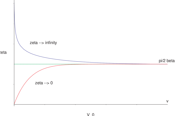
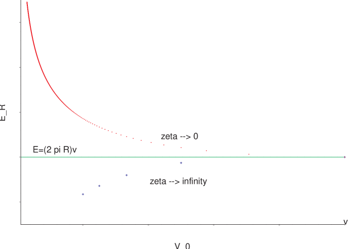
Figure 2: Schematic plots of $\zeta$ and $E_{R}$ as a function of $V_{0}$. In the RH panel, the values of $V_{0}$ are discrete due to the finite size $2\pi R$ of the circle: the exception is the horizontal line which, in both panels, corresponds to the potential $V=v/\cosh(\beta T)$. When $V_{0}\rightarrow 0$ and $\zeta\rightarrow 0$ (red curves in both figures), the energy diverges even for finite $R$ as seen in the RH panel: the lowest energy state is the one with constant vanishing $T$ and hence no kinks, as discussed in the text. Such a situation occurs for potentials of the form $V\sim e^{-T^{a}}$, $(a>1)$. If $\zeta\rightarrow\infty$ as $V_{0}\rightarrow 0$ (blue curves in both figures), the lowest energy state has the lowest value of $V_{0}$ allowed for that $R$ and corresponds to a state with one kink and anti-kink. In the limit $R\rightarrow\infty$, $V_{0}\rightarrow 0$ its energy tends to $E_{\rm Sen}.$

Now consider the case in which $\zeta\rightarrow 0$ as $V_{0}\rightarrow 0$. As discussed above, this occurs for potentials of the form

$$V=v/\cosh(T^{a})\qquad a>1,$$ (3.43)

for which $d\zeta/dV_{0}\geq 0$ for all $V_{0}$. Thus from (3.42), $dE_{R}(V_{0})/dV_{0}\leq 0$. Furthermore, as $V_{0}\rightarrow 0$, the distance between kinks and antikinks tends to zero so that $n\rightarrow\infty$ and hence $E_{R}(V_{0}\rightarrow 0)\rightarrow\infty$. This behaviour of $E_{R}$ is shown schematically in figure 2. Thus we conclude that the minimal energy solution is the one in which $V_{0}=v$ so that $T$ is constant and there are no kinks!

As we will now see, however, all these solutions for finite $R$ are in fact unstable since their spectrum of perturbations has tachyonic modes.

4 Perturbation analysis of periodic solitons on the circle

We now analyse the linear stability of the periodic solitons on the circle of radius $R$, also taking the $V_{0}\rightarrow 0$ and $R\rightarrow\infty$ limits at the end. On the circle, the solution contains an array of $n$ brane-antibranes, and hence we expect that the spectrum contains $2n$ tachyonic excitations in one to one correspondence with the annihilation channels of each brane-antibrane pair. To see this, we expand the Lagrangian to second order around a periodic soliton, ${\cal T}$, and write

$$T={\cal T}(x)+\delta T(x,t)$$

where, for simplicity, we neglect the dependence of $\delta T$ on the $p-1$ remaining directions. Then to second order

$${\cal S}^{(2)} = -\frac{V_{0}}{2}\int_{0}^{2\pi R}dx\int dt\;\left[\frac{V_{0}^{2}}{V^{2}}\left(\frac{d(\delta T)}{dx}\right)^{2}-\left(\frac{d(\delta T)}{dt}\right)^{2}+\frac{VV^{\prime}}{V_{0}^{2}}(\delta T)^{2}\right.$$ (4.1)

$$\qquad\qquad\qquad\qquad\qquad\qquad\qquad\qquad\left.+2\frac{V^{\prime}}{V}\sqrt{\frac{V^{2}}{V_{0}^{2}}-1}\delta T\frac{d(\delta T)}{dx}\right]$$

$$= -\frac{V_{0}}{2}\int_{0}^{2\pi R}dx\int dt\;\left[a({\cal T})\left(\frac{d(\delta T)}{dx}\right)^{2}+b({\cal T})(\delta T)^{2}\right].$$ (4.2)

Here, in going from (4.1) to (4.2) we have integrated by parts; $V=V({\cal T}(x))$; and

$$a=\frac{V_{0}^{2}}{V^{2}}\qquad,\qquad b=-\omega^{2}+\frac{VV^{\prime}}{V_{0}^{2}}-\frac{d}{dx}\left(\frac{V^{\prime}}{V}\sqrt{\frac{V^{2}}{V_{0}^{2}}-1}\right)$$ (4.3)

where we have supposed that

$$\delta T(x,t)=\cos(\omega t+\epsilon)\delta T(x).$$

The equation of motion is thus

$$\frac{d}{dx}\left[a\frac{d\delta T}{dx}\right]-b\delta T=0,$$

from which one can verify that

$${\delta T}=\frac{d{\cal T}}{dx}$$ (4.4)

is indeed the zero mode corresponding to translation invariance. In order to obtain a Schrödinger equation with the standard $L^{2}$ scalar product, the coefficients of the spatial and time derivatives must be equal (up to a sign) and $x$-independent. The changes of function and variable

$$dx=\frac{V_{0}}{V}dz\qquad{\rm and}\qquad\delta T=\sqrt{\frac{V}{V_{0}}}\phi$$ (4.5)

yield the Schrödinger equation

$$-\frac{d^{2}\phi}{dz^{2}}+\left(\frac{1}{\phi_{0}}\frac{d^{2}\phi_{0}}{dz^{2}}\right)\phi=\omega^{2}\phi$$ (4.6)

where, from (4.4), $\phi_{0}\propto\frac{d{\cal T}}{dx}\sqrt{\frac{V_{0}}{V}}$. Imposing that $\int\phi_{0}^{2}dz=1$ yields the normalised zero mode to be

$$\phi_{0}=\frac{\sqrt{V_{0}}}{\sqrt{E-2\pi RV_{0}}}\left(\frac{d{\cal T}}{dx}\sqrt{\frac{V_{0}}{V}}\right).$$ (4.7)

Notice that $\phi_{0}$ vanishes $2n$ times at the midpoints between the kinks and anti-kinks, whilst the potential term in (4.6) is a smooth function for all $z$. Hence we can apply Sturm-Liouville theory for periodic boundary conditions with a non-singular potential — this guarantees that the spectrum $\omega^{2}$ is discrete, and labeled by the number of zeros of the eigenfunctions. Since the zero mode possesses $2n$ zeros, we can deduce that there exists $2n$ eigenfunctions with negative $\omega^{2}$. These $2n$ eigenfunctions will be localized around the $2n$ zeros of $\phi_{0}$. For any $R$ and non-zero $V_{0}$ the kink anti-kink array is unstable.

Let us examine the $R\to\infty$ solutions whose only finite energy possibility is when $\zeta\to\infty$. One must check how the distance between the zeros of $\phi_{0}$ depends on $z$ which (rather than $x$) is the relevant variable for the Schrödinger equation. Furthermore, how does this distance depend on the behaviour of $\zeta$ as $V_{0}\rightarrow 0$? Using (4.5), the distance between zeros is $2z_{0}$ where

$$z_{0}(V_{0})=\int_{0}^{\zeta(V_{0})}\frac{V}{V_{0}}dx=\int_{0}^{T_{0}}\frac{V}{\sqrt{V^{2}-V_{0}^{2}}}dT$$ (4.8)

so that from the definition of $\zeta$,

$$z_{0}-\zeta=\int_{0}^{T_{0}}\sqrt{\frac{V-V_{0}}{V+V_{0}}}dT\;\;\longrightarrow\infty\;\;{\rm as}\;V_{0}\rightarrow 0$$ (4.9)

(again we have used the monotone convergence theorem). Thus, independently of the behaviour of $\zeta$, $z_{0}$ always diverges as $V_{0}\rightarrow 0$ and $\phi_{0}\sim\sqrt{{V(z)}/{2E_{\rm Sen}}}$: the tachyonic modes drop out of the spectrum in that limit.

5 Conclusion

We have shown that a compact dimension of radius $R$ allows the existence of time-independent and finite energy solutions of the tachyon equations derived from the DBI effective action. These solutions represent an array of kinks and anti-kinks and are unstable due to tachyonic fluctuations. Stable solutions exist in the limit of infinite separation between the kink and anti-kink. For this to be occur, three conditions must be satisfied: i) $\frac{V^{\prime}}{V}\rightarrow_{|T|\rightarrow\infty}0,$ ii) $\frac{V^{\prime}}{V^{2}}\rightarrow_{|T|\rightarrow\infty}\infty,$ iii)$\int_{0}^{\infty}V(T)dT<\infty$. The first guarantees that in the non-compact limit, the kink and anti-kink are infinitely separated. The remaining ones guarantee the finiteness of the energy.

References

- [1] J. Polchinski, Phys. Rev. Lett. 75 (1995) 4724 [hep-th/9510017].
-
[2]
A. Sen,
JHEP 9806 (1998) 007
[hep-th/9803194],
JHEP 9808 (1998) 010
[hep-th/9805019],
JHEP 9808 (1998) 012
[hep-th/9805170],
JHEP 9810 (1998) 021
[hep-th/9809111],
For reviews see:
A. Sen, hep-th/9904207; A. Lerda and R. Russo, Int. J. Mod. Phys. A 15 (2000) 771 [hep-th/9905006]. - [3] A. Sen, JHEP 9809 (1998) 023 [hep-th/9808141], JHEP 9812 (1998) 021 [hep-th/9812031].
- [4] P. Horava, Adv. Theor. Math. Phys. 2, 1373 (1999) [arXiv:hep-th/9812135].
- [5] J. M. Cline and H. Firouzjahi, arXiv:hep-th/0301101.
- [6] A. Sen, JHEP 9910, 008 (1999) [arXiv:hep-th/9909062].
- [7] M. R. Garousi, Nucl. Phys. B 584, 284 (2000) [arXiv:hep-th/0003122].
- [8] M. R. Garousi, Nucl. Phys. B 647, 117 (2002) [arXiv:hep-th/0209068].
- [9] E. A. Bergshoeff, M. de Roo, T. C. de Wit, E. Eyras and S. Panda, JHEP 0005, 009 (2000) [arXiv:hep-th/0003221].
- [10] J. Kluson, Phys. Rev. D 62, 126003 (2000) [arXiv:hep-th/0004106].
- [11] A. Sen, Mod. Phys. Lett. A 17, 1797 (2002) [arXiv:hep-th/0204143].
- [12] A. Sen, arXiv:hep-th/0209122.
- [13] D. Kutasov and V. Niarchos, arXiv:hep-th/0304045; K. Okuyama, arXiv:hep-th/0304108.
- [14] M. R. Garousi, arXiv:hep-th/0303239.
- [15] A. Sen, arXiv:hep-th/0303057.
- [16] J. A. Minahan and B. Zwiebach, JHEP 0102, 034 (2001) [arXiv:hep-th/0011226].
- [17] N. D. Lambert and I. Sachs, Phys. Rev. D 67, 026005 (2003) [arXiv:hep-th/0208217].
- [18] P. Kraus and F. Larsen, Phys. Rev. D 63, 106004 (2001) [arXiv:hep-th/0012198]; T. Takayanagi, S. Terashima and T. Uesugi, JHEP 0103, 019 (2001) [arXiv:hep-th/0012210].
- [19] R. Rajaraman, “Solitons And Instantons. An Introduction To Solitons And Instantons In Quantum Field Theory,” Amsterdam, Netherlands: North-holland ( 1982) 409p.
- [20] K. Hashimoto and N. Sakai, JHEP 0212, 064 (2002) [arXiv:hep-th/0209232].
- [21] F. Leblond and A. W. Peet, arXiv:hep-th/0303035; N. Lambert, H. Liu and J. Maldacena, arXiv:hep-th/0303139. C. Kim, Y. Kim and C. O. Lee, arXiv:hep-th/0304180.