hep-th/0304195
TU-688

Apr 2003

Effective theory for wall-antiwall system

Yutaka Sakamura

Department of Physics, Tohoku University
Sendai 980-8578, Japan

Abstract
We propose a useful method for deriving the effective theory for a system where BPS and anti-BPS domain walls coexist. Our method respects an approximately preserved SUSY near each wall. Due to the finite width of the walls, SUSY breaking terms arise at tree-level, which are exponentially suppressed. A practical approximation using the BPS wall solutions is also discussed. We show that a tachyonic mode appears in the matter sector if the corresponding mode function has a broader profile than the wall width.

1 Introduction

Supersymmetry (SUSY) is one of the most promising candidate for the solution to the hierarchy problem. When you construct a realistic model, however, SUSY must be broken because no superparticles have been observed yet. Thus, considering some SUSY breaking mechanism is an important issue for the realistic model-building. However, conventional SUSY breaking mechanisms are somewhat complicated in four dimensions [1].

On the other hand, the brane-world scenario, which was originally proposed as an alternative solution to the hierarchy problem [2, 3], has been attracted much attention and investigated in various frameworks. It is based on an idea that our four-dimensional (4D) world is embedded into a higher dimensional space-time. The 4D hypersurface on which we live is generally called a brane, and it can be a D brane (a stack of D branes) in the string theory or a topological defect in the field theory like a domain wall, vortex, monopole and so on. Recently, in spite of its original motivation of solving the hierarchy problem, the extra dimensions are utilized in order to explain various phenomenological problems, such as the fermion mass hierarchy [5, 6, 7], the proton stability [5], the doublet-triplet splitting in the grand unified theory [8] and so on. In particular, the brane-world scenario can provide some simple mechanisms of SUSY breaking. One of them is a mechanism where SUSY is broken by the boundary conditions for the bulk fields [9].

There is another interesting SUSY breaking mechanism, which utilizes BPS objects. They are the states that saturate the Bogomol’nyi-Prasad-Sommerfield (BPS) bound [11], and preserve part of the bulk SUSY. By using the (BPS) D branes, for example, we can break SUSY in a very simple way. This mechanism is called pseudo-supersymmetry [12] or quasi-supersymmetry [13]. In this mechanism, the theory has two or more sectors in which different fractions of the bulk SUSY are preserved, and all of it are broken in the whole system. One of the simplest examples is a system where parallel D3 brane and anti-D3 brane coexist with a finite distance. (See Fig.1.) Since each brane preserves an opposite half of the bulk SUSY, SUSY is completely broken in this system. A 4D effective theory for such a system can be derived by using the technique of the nonlinear realization for the space-time symmetries [12].

Figure 1: The brane configuration of the pseudo-supersymmetry.

In the field theoretical context, there is a similar SUSY breaking mechanism to the pseudo-supersymmetry. In this mechanism, SUSY is broken due to the coexistence of two BPS domain walls which preserve opposite halves of the bulk SUSY [6, 14, 15, 16]. Therefore, the corresponding field configuration is non-BPS. We will refer to such a non-BPS configuration as a wall-antiwall configuration in this paper. One of the main differences from the pseudo-supersymmetry is that the BPS walls have a finite width unlike the D-branes. Due to this wall width, SUSY breaking terms arise at tree-level in contrast to the pseudo-supersymmetry scenario where they are induced by quantum effects. In general, such a non-BPS configuration is unstable [14]. However, we can construct a stable wall-antiwall configuration by introducing a topological winding around the target space of the scalar fields [15].

When you discuss the phenomenological arguments on the wall-antiwall background, we need to derive a low-energy effective theory on it. If we eliminate the auxiliary fields of the superfields at the first step, the procedure of integrating out the massive modes becomes very complicated [17]. In the case of the BPS-wall background, this complication can be avoided by keeping a half of the bulk SUSY preserved by the wall to be manifest, i.e. by expanding the bulk superfields directly into lower-dimensional superfields for the unbroken SUSY [18]. In the case of the wall-antiwall background, however, such a way out cannot be applied because there is no SUSY preserved in the whole system. Therefore, it is difficult to derive the effective theory on such a background correctly. In Ref.[15], only mass-splitting between boson and fermion in each supermultiplet is calculated with the help of the low-energy theorem [19, 20].

In this paper, we will propose a useful method for deriving the effective theory in the wall-antiwall system. To avoid inessential complications, we will consider three-dimensional (3D) walls in a 4D bulk theory throughout this paper. Our method respects the approximately supersymmetric structure near the walls, and the resultant Lagrangian is written by the 3D superfields and the SUSY breaking terms. We can calculate all SUSY breaking parameters systematically in our method. Using this method, we will show that a tachyonic mode appears in the effective theory from the matter sector if the corresponding mode function has a broader profile than the wall width. We will also provide an approximation method using the BPS wall solutions. This approximation is useful as a practical method because the BPS wall solutions can easily be found than the non-BPS ones.

In the superstring theory, it is well-known that BPS D-branes can be described by the kink solutions in the field theory of the tachyon [21]. In particular, a D$p$ brane and anti-D$p$ brane pair is described as a wall-antiwall solution in an effective theory on a non-BPS D$(p+1)$ brane [22]. Thus, our method can also be used in the discussion of the tachyon condensation [23] in the superstring theory.

This paper is organized as follows. In the next section, we will provide useful expressions of the 4D bulk action, which respect opposite halves of the bulk SUSY. In Sect.3, we will consider the wall-antiwall configuration and derive the 3D effective theory. A practical approximation method is provided in Sect.4. In Sect.5, we will demonstrate our method in an explicit example of the stable wall-antiwall configuration. We will also discuss the gauge interactions in Sect.6. Sect.7 is devoted to the summary and the discussion. Notations and some useful properties of the classical background are listed in the appendices.

2 Useful expressions of the bulk action

We will consider the following Wess-Zumino model as a 4D ${\cal N}=1$ bulk theory.

$$S=\int\!\!{\rm d}^{4}x{\rm d}^{2}\theta{\rm d}^{2}\bar{\theta}\>\bar{\Phi}\Phi+\int\!\!{\rm d}^{4}x{\rm d}^{2}\theta\>W(\Phi)+\int\!\!{\rm d}^{4}x{\rm d}^{2}\bar{\theta}\>\bar{W}(\bar{\Phi}),$$ (1)

where

$$\Phi(y^{\mu},\theta)=A(y^{\mu})+\sqrt{2}\theta\Psi(y^{\mu})+\theta^{2}F(y^{\mu})\;\;\;\;\;(y^{\mu}\equiv x^{\mu}+i\theta\sigma^{\mu}\bar{\theta})$$ (2)

is a chiral superfield.

Here, we decompose the Grassmann coordinates $\theta$ and $\bar{\theta}$ as

$$\theta^{\alpha}=\frac{e^{i\delta/2}}{\sqrt{2}}(\theta_{2}^{\alpha}+i\theta_{1}^{\alpha}),\;\;\;\bar{\theta}^{\dot{\alpha}}=\frac{e^{-i\delta/2}}{\sqrt{2}}(\theta_{2}^{\alpha}-i\theta_{1}^{\alpha}),$$ (3)

where $\delta$ is a constant phase. Corresponding to this decomposition, we also decompose the supercharges $Q_{\alpha}$ and $\bar{Q}_{\dot{\alpha}}$ as

$$Q_{\alpha}=\frac{e^{-i\delta/2}}{\sqrt{2}}(Q_{2\alpha}-iQ_{1\alpha}),\;\;\;\bar{Q}_{\dot{\alpha}}=-(Q_{\alpha})^{*}=-\frac{e^{i\delta/2}}{\sqrt{2}}(Q_{2\alpha}+iQ_{1\alpha}).$$ (4)

Then, it follows that

$$\theta Q+\bar{\theta}\bar{Q}=\theta_{1}Q_{1}+\theta_{2}Q_{2}.$$ (5)

Under the above decomposition, the 4D ${\cal N}=1$ SUSY algebra can be rewritten as

$$\left\{Q_{1\alpha},Q_{1\beta}\right\}\!\!\! =\!\!\! \left\{Q_{2\alpha},Q_{2\beta}\right\}=2\left(\gamma_{(3)}^{m}\sigma^{2}\right)_{\alpha\beta}P_{m},$$

$$\left\{Q_{1\alpha},Q_{2\beta}\right\}\!\!\! =\!\!\! -\left\{Q_{2\alpha},Q_{1\beta}\right\}=-2i\left(\sigma^{2}\right)_{\alpha\beta}P_{2}.$$ (6)

This can be interpreted as the central extended 3D ${\cal N}=2$ SUSY algebra if we identify $P_{2}$ with the central charge.

Now, if we perform an integration for $\theta_{2}$ in Eq.(1), we can obtain the following expression [18].

$$S=\int\!\!{\rm d}^{3}x{\rm d}^{2}\theta_{1}{\rm d}x_{2}\>\left\{D_{1}^{\alpha}\bar{\varphi}^{(1)}D_{1\alpha}\varphi^{(1)}+{\rm Im}\left(2\bar{\varphi}^{(1)}\partial_{2}\varphi^{(1)}+4e^{-i\delta}W(\varphi^{(1)})\right)\right\},$$ (7)

where $\partial_{2}\equiv\partial/\partial x_{2}$, $D_{1\alpha}\equiv\partial/\partial\theta_{1}^{\alpha}-i(\gamma_{(3)}^{m}\theta_{1})_{\alpha}\partial_{m}$ is a covariant spinor derivative for $Q_{1}$-SUSY, and

$$\varphi^{(1)}(x^{m},x_{2},\theta_{1})\!\!\! \equiv\!\!\! e^{\theta_{1}Q_{1}}\times A(x^{m},x_{2})$$ (8)

$$=\!\!\! A+e^{i\delta/2}(\sigma^{2})_{\alpha\beta}\theta_{1}^{\alpha}\Psi^{\beta}+\frac{i}{2}\theta_{1}^{2}(\partial_{2}A+e^{i\delta}F).$$

Throughout this paper, $m=0,1,3$ denotes the 3D Lorentz index, and the $x_{2}$-direction is chosen as the extra dimension. The relation between $\varphi^{(1)}$ and the original chiral superfield $\Phi$ is given by

$$\Phi(y^{\mu},\theta)=e^{-\theta_{1}\theta_{2}\partial_{2}}e^{-i\theta_{2}D_{1}+i\theta_{2}^{2}\partial_{2}}\varphi^{(1)}(x^{m},x_{2},\theta_{1}).$$ (9)

On the other hand, if we perform an integration for $\theta_{1}$, Eq.(1) becomes

$$S=\int\!\!{\rm d}^{3}x{\rm d}^{2}\theta_{2}{\rm d}x_{2}\>\left\{D_{2}^{\alpha}\bar{\varphi}^{(2)}D_{2\alpha}\varphi^{(2)}+{\rm Im}\left(2\bar{\varphi}^{(2)}\partial_{2}\varphi^{(2)}-4e^{-i\delta}W(\varphi^{(2)})\right)\right\},$$ (10)

where $D_{2\alpha}\equiv\partial/\partial\theta_{2}^{\alpha}-i(\gamma_{(3)}^{m}\theta_{2})_{\alpha}\partial_{m}$ is a covariant spinor derivative for $Q_{2}$-SUSY, and

$$\varphi^{(2)}(x^{m},x_{2},\theta_{2})\!\!\! \equiv\!\!\! e^{\theta_{2}Q_{2}}\times A(x^{m},x_{2})$$ (11)

$$=\!\!\! A-ie^{i\delta/2}(\sigma^{2})_{\alpha\beta}\theta_{2}^{\alpha}\Psi^{\beta}+\frac{i}{2}\theta_{2}^{2}(\partial_{2}A-e^{i\delta}F).$$

The relation between $\varphi^{(2)}$ and $\Phi$ is given by

$$\Phi(y^{\mu},\theta)=e^{\theta_{1}\theta_{2}\partial_{2}}e^{i\theta_{1}D_{2}+i\theta_{1}^{2}\partial_{2}}\varphi^{(2)}(x^{m},x_{2},\theta_{2}).$$ (12)

From Eqs.(9) and (12), we can obtain the relation between $\varphi^{(1)}$ and $\varphi^{(2)}$ as follows.

$$\varphi^{(1)}(x^{m},x_{2},\theta_{1})\!\!\! =\!\!\! \Phi|_{\theta_{2}=0}=e^{i\theta_{1}D_{2}+i\theta_{1}\partial_{2}}\varphi^{(2)}|_{\theta_{2}=0}$$ (13)

$$=\!\!\! \varphi^{(2)}(x^{m},x_{2}+i\theta_{1}^{2},i\theta_{1})$$

In fact, we can explicitly show that

$$\int\!\!{\rm d}^{2}\theta_{1}{\rm d}x_{2}\>\left\{D_{1}^{\alpha}\left(\bar{\varphi}^{(2)}(x^{m},x_{2}-i\theta_{1}^{2},-i\theta_{1})\right)D_{1\alpha}\left(\varphi^{(2)}(x^{m},x_{2}+i\theta_{1}^{2},i\theta_{1})\right)\right.$$ (14)

$$\hskip 71.13188pt\left.+{\rm Im}\left(2\bar{\varphi}^{(2)}(x^{m},x_{2}-i\theta_{1}^{2},-i\theta_{1})\partial_{2}\left(\varphi^{(2)}(x^{m},x_{2}+i\theta_{1}^{2},i\theta_{1})\right)\right)\right\}$$

$$=\!\!\! \int\!\!{\rm d}^{2}\theta_{2}{\rm d}x_{2}\>\left\{D_{2}^{\alpha}\bar{\varphi}^{(2)}D_{2\alpha}\varphi^{(2)}+{\rm Im}\left(2\bar{\varphi}^{(2)}\partial_{2}\varphi^{(2)}\right)\right\},$$

and

$$\int\!\!{\rm d}^{2}\theta_{1}{\rm d}x_{2}\>{\rm Im}\left(e^{-i\delta}W(\varphi^{(2)}(x^{m},x_{2}+i\theta_{1}^{2},i\theta_{1}))\right)=\int\!\!{\rm d}^{2}\theta_{2}{\rm d}x_{2}\>{\rm Im}\left(-e^{-i\delta}W(\varphi^{(2)})\right).$$ (15)

Namely, we can derive Eq.(10) by substituting Eq.(13) into Eq.(7).

3 Wall-antiwall system

3.1 Classical field configuration

Let us assume that the bulk theory (1) has two supersymmetric vacua $A=A_{\rm I}$ and $A=A_{\rm II}$, and that there exists a BPS domain wall configuration $A=A_{\rm cl1}(x_{2})$ which interpolates between them. That is,

$$A_{\rm cl1}(-\infty)=A_{\rm I},\;\;\;A_{\rm cl1}(\infty)=A_{\rm II},$$ (16)

and $A_{\rm cl1}(x_{2})$ satisfies a BPS equation

$$\partial_{2}A_{\rm cl1}=e^{i\delta}\bar{W}^{\prime}(\bar{A}_{\rm cl1}),$$ (17)

where a prime denotes a differentiation for the argument, and

$$\delta\equiv\arg\left(W(A_{\rm II})-W(A_{\rm I})\right).$$ (18)

If we take this value of $\delta$ as that in the decompositions (3) and (4), $Q_{1}$ and $Q_{2}$ correspond to the unbroken and broken supercharges respectively.

When the theory has the BPS domain wall $A_{\rm cl1}(x_{2})$, it also has the “anti-BPS” domain wall $A=A_{\rm cl2}(x_{2})$. That is,

$$A_{\rm cl2}(-\infty)=A_{\rm II},\;\;\;A_{\rm cl2}(\infty)=A_{\rm I},$$ (19)

and the BPS equation for $A_{\rm cl2}(x_{2})$ is

$$\partial_{2}A_{\rm cl2}=-e^{i\delta}\bar{W}^{\prime}(\bar{A}_{\rm cl2}).$$ (20)

This anti-BPS wall preserves $Q_{2}$-SUSY and breaks $Q_{1}$-SUSY.

Now we will consider a system in which the above two kinds of BPS walls coexist. Since the two walls preserve opposite halves of the bulk SUSY, All of it are broken in such a system. That is, a corresponding field configuration $A_{\rm cl}(x_{2})$ is non-BPS. Unlike the BPS wall, such a non-BPS configuration is usually unstable [14]. However, we can construct a stable non-BPS configuration by introducing the topological winding around the target space of the scalar field $A(x_{2})$ [15]. We will discuss an explicit example of such a stable configuration in Sect.5. In the following, we will assume that the extra dimension ($x_{2}$-direction) is compactified on $S^{1}$ with radius $R$.

Furthermore, to simplify the discussions, we will also assume that the superpotential $W$ has the following symmetric property.

$$W^{\prime}(A-A_{\rm M})=W^{\prime}(A_{\rm M}-A),$$ (21)

where $A_{\rm M}\equiv(A_{\rm I}+A_{\rm II})/2$ is a middle point between the two vacua on the target space. Under this assumption, the BPS and anti-BPS walls are located at antipodal points on $S^{1}$, and $A_{\rm cl}(x_{2})$ has the following property. (See Fig.3 in Sect.5.)

$$\partial_{2}A_{\rm cl}(x_{2}-\pi R)\!\!\! =\!\!\! \pm\partial_{2}A_{\rm cl}(x_{2}),$$

$$W^{\prime}(A_{\rm cl}(x_{2}-\pi R))\!\!\! =\!\!\! \mp W^{\prime}(A_{\rm cl}(x_{2})).$$ (22)

The upper signs in R.H.S correspond to the case of a stable configuration with the topological winding [15], and the lower signs correspond to the case of an unstable configuration with no winding [14]. From now on, we will choose the origin of the coordinate $x_{2}$ so that the (approximate) BPS wall is located at $x_{2}=0$ and the anti-BPS wall is at $x_{2}=\pi R$.

3.2 Mode-expansion

First, we will consider the mode-expansion of $\varphi^{(1)}$ in Eq.(7). The classical background of $\varphi^{(1)}$ is

$$\varphi_{\rm cl}^{(1)}(x_{2},\theta_{1})\!\!\! =\!\!\! e^{\theta_{1}Q_{1}}\times A_{\rm cl}(x_{2})=A_{\rm cl}(x_{2})+\frac{i}{2}\theta_{1}^{2}\left(\partial_{2}A_{\rm cl}(x_{2})+e^{i\delta}F_{\rm cl}(x_{2})\right)$$ (23)

$$=\!\!\! A_{\rm cl}(x_{2})+\frac{i}{2}\theta_{1}^{2}\left(\partial_{2}A_{\rm cl}(x_{2})-e^{i\delta}\bar{W}^{\prime}(\bar{A}_{\rm cl}(x_{2}))\right).$$

Here we used the equation of motion for the auxiliary field $F$ in the last equation.

Similarly, the background of $\varphi^{(2)}$ is

$$\varphi_{\rm cl}^{(2)}(x_{2},\theta_{2})=e^{\theta_{2}Q_{2}}\times A_{\rm cl}(x_{2})=A_{\rm cl}(x_{2})+\frac{i}{2}\theta_{2}^{2}\left(\partial_{2}A_{\rm cl}(x_{2})+e^{i\delta}\bar{W}^{\prime}(\bar{A}_{\rm cl}(x_{2}))\right).$$ (24)

The superfield equation of motion

$$-\frac{1}{4}\bar{D}^{2}\bar{\Phi}+W^{\prime}(\Phi)=0$$ (25)

can be rewritten in terms of $\varphi^{(1)}$ as [18]

$$-\frac{1}{2}D_{1}^{2}\bar{\varphi}^{(1)}+i\partial_{2}\bar{\varphi}^{(1)}-ie^{-i\delta}W^{\prime}(\varphi^{(1)})=0.$$ (26)

By substituting $\varphi^{(1)}=\varphi_{\rm cl}^{(1)}+\tilde{\varphi}^{(1)}$ into Eq.(26) and using the equation of motion for $\varphi_{\rm cl}^{(1)}$, we can obtain the linearized equation of motion for the fluctuation field $\tilde{\varphi}^{(1)}$ as

$$-\frac{1}{2}D_{1}^{2}\bar{\tilde{\varphi}}^{(1)}+i\partial_{2}\bar{\tilde{\varphi}}^{(1)}-ie^{-i\delta}W^{\prime\prime}(\varphi_{\rm cl}^{(1)})\tilde{\varphi}^{(1)}=0.$$ (27)

Let us denote the component fields of $\tilde{\varphi}^{(1)}$ as

$$\tilde{\varphi}^{(1)}=a^{(1)}+\theta_{1}\psi^{(1)}+\frac{1}{2}\theta_{1}^{2}f^{(1)}.$$ (28)

Then, we can obtain the following linearized equation of motion for $\psi^{(1)}_{\alpha}$ by picking up linear terms for $\theta_{1}$ from Eq.(27).

$$-i\left(\gamma_{(3)}^{m}\partial_{m}\bar{\psi}^{(1)}\right)_{\alpha}+i\left\{\partial_{2}\bar{\psi}^{(1)}_{\alpha}-e^{-i\delta}W^{\prime\prime}(A_{\rm cl})\psi^{(1)}_{\alpha}\right\}=0.$$ (29)

Therefore, the mode equation for $\psi^{(1)}_{\alpha}$ can be read off as

$$i\left\{\partial_{2}\bar{u}^{(1)}_{(n)}-e^{-i\delta}W^{\prime\prime}(A_{\rm cl})u^{(1)}_{(n)}\right\}=m_{(n)}\bar{u}^{(1)}_{(n)},$$ (30)

where $m_{(n)}$ are eigenvalues. Note that this has a very similar form to that of the BPS-wall case [18]. The only difference is that the argument of $W^{\prime\prime}$ is a non-BPS configuration $A_{\rm cl}$, instead of $A_{\rm cl1}$. On the other hand, the mode equation for $a^{(1)}$ receives more corrections than that for $\psi^{(1)}_{\alpha}$ when you change the background from the BPS one to the non-BPS one. Therefore, it is convenient to use the mode functions of $\psi^{(1)}_{\alpha}$ in the following derivation of the 3D effective theory.

To simplify the discussion, we will consider a case that $A_{\rm cl}(x_{2})$ and all parameters of the 4D bulk theory are real. In this case, $\delta=0$ and the mode equation (30) can be rewritten as

$$\left\{-\partial_{2}+W^{\prime\prime}(A_{\rm cl})\right\}u_{{\rm R}(n)}\!\!\! =\!\!\! m_{(n)}u_{{\rm I}(n)},$$

$$\left\{\partial_{2}+W^{\prime\prime}(A_{\rm cl})\right\}u_{{\rm I}(n)}\!\!\! =\!\!\! m_{(n)}u_{{\rm R}(n)},$$ (31)

where $u_{{\rm R}(n)}(x_{2})$ and $u_{{\rm I}(n)}(x_{2})$ are defined by

$$u^{(1)}_{(n)}=\frac{1}{\sqrt{2}}(u_{{\rm R}(n)}+iu_{{\rm I}(n)}).$$ (32)

Using these mode functions, $\psi^{(1)}_{\alpha}$ can be expanded into 3D fields as

$$\psi^{(1)}_{\alpha}(x^{m},x_{2})=\frac{1}{\sqrt{2}}\sum_{n=0}^{\infty}\left(u_{{\rm R}(n)}(x_{2})\psi_{{\rm R}(n)\alpha}(x^{m})+iu_{{\rm I}(n)}(x_{2})\psi_{{\rm I}(n)\alpha}(x^{m})\right).$$ (33)

Here, note that the mode equation (31) has two zero-modes,

$$u_{{\rm R}(0)}(x_{2})\!\!\! =\!\!\! C_{0}\,e^{\int_{0}^{x_{2}}\!{\rm d}y\>W^{\prime\prime}(A_{\rm cl}(y))},$$

$$u_{{\rm I}(0)}(x_{2})\!\!\! =\!\!\! C_{0}\,e^{-\int_{\pi R}^{x_{2}}\!{\rm d}y\>W^{\prime\prime}(A_{\rm cl}(y))},$$ (34)

where $C_{0}$ is a common normalization factor. The corresponding fields $\psi_{{\rm R}(0)}$ and $\psi_{{\rm I}(0)}$ are the goldstinos for the broken $Q_{2}$- and $Q_{1}$-SUSY, and localized on the (approximate) BPS and anti-BPS walls, respectively. Therefore, it is convenient to introduce the following 3D superfields.

$$\varphi^{(1)}_{(0)}(x^{m},\theta_{1})\!\!\! =\!\!\! a^{(1)}_{(0)}(x^{m})+\theta_{1}\psi_{{\rm R}(0)}(x^{m})+\frac{1}{2}\theta_{1}^{2}f^{(1)}_{(0)}(x^{m}),$$

$$\varphi^{(2)}_{(0)}(x^{m},\theta_{2})\!\!\! =\!\!\! a^{(2)}_{(0)}(x^{m})+\theta_{2}\psi_{{\rm I}(0)}(x^{m})+\frac{1}{2}\theta_{2}^{2}f^{(2)}_{(0)}(x^{m}).$$ (35)

Considering Eqs.(13) and (33), the mode-expansion of the fluctuation field $\tilde{\varphi}^{(1)}$ can be expressed as

$$\tilde{\varphi}^{(1)}(x^{m},x_{2},\theta_{1})\!\!\! =\!\!\! \frac{1}{\sqrt{2}}\left\{u_{{\rm R}(0)}(x_{2})\varphi^{(1)}_{(0)}(x^{m},\theta_{1})+u_{{\rm I}(0)}(x_{2}+i\theta_{1}^{2})\varphi^{(2)}_{(0)}(x^{m},i\theta_{1})\right\}$$ (36)

$$+(\mbox{massive modes}).$$

Strictly speaking, the bosonic component of this expression deviates the correct mode-expansion because we used the mode functions of $\psi^{(1)}_{\alpha}$. However, this deviation is negligibly small when the distance between the walls is large enough On the other hand, the massive modes cannot be well described by using 3D superfields because they have broadly spread profiles along the $x_{2}$-direction and thus receive large SUSY breaking effects.

3.3 Derivation of 3D effective theory

In the following, we will concentrate ourselves on the low-energy region where all massive modes are decoupled, and will drop them from expressions. By substituting the expression

$$\varphi^{(1)}(x^{m},x_{2},\theta_{1})\!\!\! =\!\!\! \varphi_{\rm cl}^{(1)}(x_{2},\theta_{1})$$ (37)

$$+\frac{1}{\sqrt{2}}\left\{u_{{\rm R}(0)}(x_{2})\varphi^{(1)}_{(0)}(x^{m},\theta_{1})+u_{{\rm I}(0)}(x_{2}+i\theta_{1}^{2})\varphi^{(2)}_{(0)}(x^{m},i\theta_{1})\right\}$$

into Eq.(7) and carrying out the $x_{2}$-integration, we can obtain the 3D effective theory.

A zero-th order term for the fields, i.e. the cosmological constant term, can be calculated as

$${\cal L}_{\rm cc}^{(3)}\!\!\! =\!\!\! \int\!\!{\rm d}^{2}\theta_{1}{\rm d}x_{2}\>\left\{D_{1}^{\alpha}\bar{\varphi}_{\rm cl}^{(1)}D_{1\alpha}\varphi_{\rm cl}^{(1)}+{\rm Im}\left(2\bar{\varphi}_{\rm cl}^{(1)}\partial_{2}\varphi_{\rm cl}^{(1)}+4W(\varphi_{\rm cl}^{(1)})\right)\right\}$$ (38)

$$=\!\!\! -\int\!\!{\rm d}x_{2}\>\left\{(\partial_{2}A_{\rm cl})^{2}+\left(W^{\prime}(A_{\rm cl})\right)^{2}\right\}=-V_{0},$$

where $V_{0}$ is an energy (per unit area) of the background field configuration $A_{\rm cl}(x_{2})$.

Linear terms for the fields are cancelled due to the equation of motion for $\varphi_{\rm cl}^{(1)}$.

Then, we will calculate quadratic terms for the fields.

$${\cal L}_{\rm quad}^{(3)}\!\!\! =\!\!\! \int\!\!{\rm d}^{2}\theta_{1}{\rm d}x_{2}\>\left\{D_{1}^{\alpha}\bar{\tilde{\varphi}}^{(1)}D_{1\alpha}\tilde{\varphi}^{(1)}-2{\rm Im}\left(\tilde{\varphi}^{(1)}\left(\partial_{2}\bar{\tilde{\varphi}}^{(1)}-W^{\prime\prime}(\varphi_{\rm cl}^{(1)})\tilde{\varphi}^{(1)}\right)\right)\right\}$$ (39)

$$=\!\!\! \int\!\!{\rm d}^{2}\theta_{1}\>\frac{1}{2}\left(D_{1}\varphi^{(1)}_{(0)}\right)^{2}+\int\!\!{\rm d}^{2}\theta_{2}\>\frac{1}{2}\left(D_{2}\varphi^{(2)}_{(0)}\right)^{2}$$

$$-\eta\left(f^{(1)}_{(0)}f^{(2)}_{(0)}+\partial^{m}a^{(1)}_{(0)}\partial_{m}a^{(2)}_{(0)}\right)-\frac{1}{2}m_{0}^{2}\left(a^{(1)}_{(0)}-a^{(2)}_{(0)}\right)^{2},$$

where $\eta\equiv\int{\rm d}x_{2}\>u_{{\rm R}(0)}u_{{\rm I}(0)}$ is a dimensionless number, which is exponentially suppressed in terms of the wall distance $\pi R$, and the scalar mass parameter $m_{0}^{2}$ is defined as

$$m_{0}^{2}\!\!\! \equiv\!\!\! -\int\!\!{\rm d}x_{2}\>W^{\prime\prime\prime}(A_{\rm cl})U_{{\rm I}0}u_{{\rm R}(0)}^{2}=\int\!\!{\rm d}x_{2}\>W^{\prime\prime\prime}(A_{\rm cl})U_{{\rm R}0}u_{{\rm I}(0)}^{2}$$ (40)

$$=\!\!\! \int\!\!{\rm d}x_{2}\>W^{\prime\prime\prime}(A_{\rm cl})U_{{\rm I}0}u_{{\rm R}(0)}u_{{\rm I}(0)}=-\int\!\!{\rm d}x_{2}\>W^{\prime\prime\prime}(A_{\rm cl})U_{{\rm R}0}u_{{\rm R}(0)}u_{{\rm I}(0)},$$

Here, we have used the formulae Eqs.(14) and (15), and the functions $U_{{\rm R}0}(x_{2})$ and $U_{{\rm I}0}(x_{2})$ are defined as

$$U_{{\rm R}0}(x_{2})\!\!\! \equiv\!\!\! \partial_{2}A_{\rm cl}(x_{2})+W^{\prime}(A_{\rm cl}(x_{2})),$$

$$U_{{\rm I}0}(x_{2})\!\!\! \equiv\!\!\! \partial_{2}A_{\rm cl}(x_{2})-W^{\prime}(A_{\rm cl}(x_{2})),$$ (41)

which are contained in $\varphi_{\rm cl}^{(1)}$ and $\varphi_{\rm cl}^{(2)}$ as

$$\varphi_{\rm cl}^{(1)}(x_{2},\theta_{1})\!\!\! =\!\!\! A_{\rm cl}(x_{2})+\frac{i}{2}\theta_{1}^{2}U_{{\rm I}0}(x_{2}),$$

$$\varphi_{\rm cl}^{(2)}(x_{2},\theta_{2})\!\!\! =\!\!\! A_{\rm cl}(x_{2})+\frac{i}{2}\theta_{2}^{2}U_{{\rm R}0}(x_{2}).$$ (42)

Note that $U_{{\rm R}0}(x_{2})$ and $U_{{\rm I}0}(x_{2})$ satisfy the mode equations (31) with $m_{(n)}=0$, and are related to $u_{{\rm R}(0)}(x_{2})$ and $u_{{\rm I}(0)}(x_{2})$ as

$$U_{{\rm R}0}(x_{2})=\sqrt{V_{0}}\,u_{{\rm R}(0)}(x_{2}),\;\;\;U_{{\rm I}0}(x_{2})=\sqrt{V_{0}}\,u_{{\rm I}(0)}(x_{2}).$$ (43)

Equalities in Eq.(40) are followed from this relation and Eqs. (146) and (150) in Appendix B.

From Eqs.(38) and (39), the bosonic part of the 3D Lagrangian ${\cal L}^{(3)}$ is

$${\cal L}^{(3)}_{\rm bosonic}\!\!\! =\!\!\! -V_{0}-\frac{1}{2}(\partial^{m}a^{(1)}_{(0)},\partial^{m}a^{(2)}_{(0)})\left(\begin{array}[]{cc}1&\eta\\ \eta&1\end{array}\right)\left(\begin{array}[]{c}\partial_{m}a^{(1)}_{(0)}\\ \partial_{m}a^{(2)}_{(0)}\end{array}\right)$$ (58)

$$-\frac{1}{2}(a^{(1)}_{(0)},a^{(2)}_{(0)})\left(\begin{array}[]{cc}m_{0}^{2}&-m_{0}^{2}\\ -m_{0}^{2}&m_{0}^{2}\end{array}\right)\left(\begin{array}[]{c}a^{(1)}_{(0)}\\ a^{(2)}_{(0)}\end{array}\right)+\frac{1}{2}(f^{(1)}_{(0)},f^{(2)}_{(0)})\left(\begin{array}[]{cc}1&-\eta\\ -\eta&1\end{array}\right)\left(\begin{array}[]{c}f^{(1)}_{(0)}\\ f^{(2)}_{(0)}\end{array}\right)$$

$$+(\mbox{interaction terms}).$$

Then, canonically normalized scalar fields are

$$a_{+(0)}\!\!\! \equiv\!\!\! \sqrt{\frac{1+\eta}{2}}\left(a^{(1)}_{(0)}+a^{(2)}_{(0)}\right),$$

$$a_{-(0)}\!\!\! \equiv\!\!\! \sqrt{\frac{1-\eta}{2}}\left(a^{(1)}_{(0)}-a^{(2)}_{(0)}\right).$$ (59)

For the auxiliary fields, we redefine them as

$$f_{+(0)}\!\!\! \equiv\!\!\! \sqrt{\frac{1-\eta}{2}}\left(f^{(1)}_{(0)}+f^{(2)}_{(0)}\right),$$

$$f_{-(0)}\!\!\! \equiv\!\!\! \sqrt{\frac{1+\eta}{2}}\left(f^{(1)}_{(0)}-f^{(2)}_{(0)}\right).$$ (60)

Using these fields, Eq.(58) can be rewritten as

$${\cal L}^{(3)}_{\rm bosonic}\!\!\! =\!\!\! -V_{0}-\frac{1}{2}\partial^{m}a_{+(0)}\partial_{m}a_{+(0)}-\frac{1}{2}\partial^{m}a_{-(0)}\partial_{m}a_{-(0)}-\frac{1}{2}\left(\frac{2m_{0}^{2}}{1-\eta}\right)a_{-(0)}^{2}$$ (61)

$$+\frac{1}{2}f_{+(0)}^{2}+\frac{1}{2}f_{-(0)}^{2}+(\mbox{interaction terms}).$$

Notice that the massless mode $a_{+(0)}(x^{m})$ is the Nambu-Goldstone mode for the translation along the $x_{2}$-direction. In fact, the mode function of $a_{+(0)}(x^{m})$ is

$$u_{+(0)}(x_{2})\!\!\! =\!\!\! \frac{1}{\sqrt{2(1-\eta)}}\left(u_{{\rm R}(0)}(x_{2})+u_{{\rm I}(0)}(x_{2})\right)$$ (62)

$$\frac{1}{\sqrt{2(1-\eta)V_{0}}}\left(U_{{\rm R}0}(x_{2})+U_{{\rm I}0}(x_{2})\right)=\sqrt{\frac{2}{(1-\eta)V_{0}}}\,\partial_{2}A_{\rm cl}(x_{2}).$$

This mode function is correctly normalized as expected.

$$\int\!\!{\rm d}x_{2}\>u_{+(0)}^{2}=1.$$ (63)

We can calculate interaction terms in a similar way. For example, cubic couplings are obtained as

$${\cal L}^{(3)}_{\rm cubic}\!\!\! =\!\!\! \int\!\!{\rm d}^{2}\theta_{1}{\rm d}x_{2}\>4{\rm Im}\left\{\frac{1}{3!}W^{\prime\prime\prime}(\varphi_{\rm cl}^{(1)})\tilde{\varphi}^{3}\right\}$$ (64)

$$=\!\!\! {\cal A}_{111}\left(a^{(1)}_{(0)}\right)^{3}+{\cal A}_{112}\left(a^{(1)}_{(0)}\right)^{2}a^{(2)}_{(0)}+{\cal A}_{122}a^{(1)}_{(0)}\left(a^{(2)}_{(0)}\right)^{2}+{\cal A}_{222}\left(a^{(2)}_{(0)}\right)^{3}$$

$$+\frac{g_{(-{\rm RI})}}{\sqrt{2}}\left(a^{(1)}_{(0)}-a^{(2)}_{(0)}\right)\psi_{{\rm R}(0)}\psi_{{\rm I}(0)},$$

where

$${\cal A}_{111}\!\!\! \equiv\!\!\! \frac{1}{6\sqrt{2}}\int\!\!{\rm d}x_{2}\>W^{\prime\prime\prime}(A_{\rm cl})U_{{\rm I}0}u_{{\rm R}(0)}^{3},$$

$${\cal A}_{112}\!\!\! \equiv\!\!\! \frac{1}{\sqrt{2}}\int\!\!{\rm d}x_{2}\>\left\{W^{\prime\prime\prime}(A_{\rm cl})u_{{\rm R}(0)}^{2}\partial_{2}u_{{\rm I}(0)}+\frac{1}{2}W^{\prime\prime\prime\prime}(A_{\rm cl})U_{{\rm I}0}u_{{\rm R}(0)}^{2}u_{{\rm I}(0)}\right\},$$

$${\cal A}_{122}\!\!\! \equiv\!\!\! \frac{1}{\sqrt{2}}\int\!\!{\rm d}x_{2}\>\left\{W^{\prime\prime\prime}(A_{\rm cl})u_{{\rm I}(0)}^{2}\partial_{2}u_{{\rm R}(0)}+\frac{1}{2}W^{\prime\prime\prime\prime}(A_{\rm cl})U_{{\rm R}0}u_{{\rm I}(0)}^{2}u_{{\rm R}(0)}\right\},$$

$${\cal A}_{222}\!\!\! \equiv\!\!\! \frac{1}{6\sqrt{2}}\int\!\!{\rm d}x_{2}\>W^{\prime\prime\prime}(A_{\rm cl})U_{{\rm R}0}u_{{\rm I}(0)}^{3},$$ (65)

$$g_{(-{\rm RI})}\!\!\! \equiv\!\!\! -\int\!\!{\rm d}x_{2}\>W^{\prime\prime\prime}(A_{\rm cl})u_{{\rm R}(0)}^{2}u_{{\rm I}(0)}=\int\!\!{\rm d}x_{2}\>W^{\prime\prime\prime}(A_{\rm cl})u_{{\rm I}(0)}^{2}u_{{\rm R}(0)}.$$ (66)

The second equality in Eq.(66) is followed from the relations (43), (146) and (150).

The “$A$-terms” for ${\cal A}_{111}$ and ${\cal A}_{222}$ correspond to Eq.(3.3) in Ref.[15], but terms for ${\cal A}_{112}$ and ${\cal A}_{122}$ were missed there.

Notice that the above cubic couplings are all SUSY breaking terms. In fact, we can easily show that there are no supersymmetric couplings in the effective theory. This stems from the assumption that $A_{\rm cl}(x_{2})$ and all parameters in the bulk theory are real. As will be seen in the next section, supersymmetric interaction terms appear in the effective theory if we introduce a complex coupling constant in the bulk theory.

The existence of the last Yukawa coupling term in Eq.(64) is expected from the low-energy theorem [19, 20], which predicts the relation among the Yukawa coupling constant $g_{(-RI)}$, the mass-splitting between the bosonic and fermionic modes $m_{0}^{2}$ and an order parameter of SUSY breaking $\sqrt{V_{0}}$ as

$$g_{(-{\rm RI})}=\frac{m_{0}^{2}}{\sqrt{V_{0}}}.$$ (67)

This relation can easily be seen from Eqs.(40), (43) and (66) in our approach.

3.4 Matter fields

In order to construct a more realistic model, we need to introduce matter fields, which do not contribute to the domain wall configuration. Here, we will introduce an extra chiral superfield $X$ as matter fields whose interactions are given by

$$W_{\rm int}(\Phi,X)=\frac{\alpha}{2}W^{\prime\prime}(\Phi)X^{2}+\beta X^{3},$$ (68)

where constants $\alpha$ and $\beta$ are positive and complex, respectively. The first term in Eq.(68) is required in order to localize the lowest modes of $X$ on the walls, and the second term provides interactions among the matter fields, which are important when we discuss the phenomenology. The component fields of $X$ are denoted as

$$X(y,\theta)=A_{X}(y)+\sqrt{2}\theta\Psi_{X}(y)+\theta^{2}F_{X}(y).$$ (69)

We will assume that $A_{X}(x)$ does not have a nontrivial background, i.e. $A_{X{\rm cl}}=0$. The corresponding field to $\varphi^{(1)}$ in Eq.(8) is

$$\varphi^{(1)}_{X}(x^{m},x_{2},\theta_{1})\!\!\! \equiv\!\!\! e^{\theta_{1}Q_{1}}\times A_{X}(x^{m},x_{2})$$ (70)

$$=\!\!\! a^{(1)}_{X}(x^{m},x_{2})+\theta_{1}\psi^{(1)}_{X}(x^{m},x_{2})+\frac{1}{2}\theta_{1}^{2}f^{(1)}_{X}(x^{m},x_{2}).$$

The mode equations for the fermionic component $\psi^{(1)}_{X\alpha}$ can be obtained in the same way as the derivation of Eq.(31).

$$\left\{-\partial_{2}+\alpha W^{\prime\prime}(A_{\rm cl})\right\}u_{{\rm R}X(n)}\!\!\! =\!\!\! m_{X(n)}u_{{\rm I}X(n)},$$

$$\left\{\partial_{2}+\alpha W^{\prime\prime}(A_{\rm cl})\right\}u_{{\rm I}X(n)}\!\!\! =\!\!\! m_{X(n)}u_{{\rm R}X(n)},$$ (71)

where $m_{X(n)}$ are eigenvalues. Using solutions of these equations, $\psi^{(1)}_{X\alpha}$ can be expanded as

$$\psi^{(1)}_{X\alpha}(x^{m},x_{2})=\frac{1}{\sqrt{2}}\sum_{n=0}^{\infty}\left\{u_{{\rm R}X(n)}(x_{2})\psi_{{\rm R}(n)\alpha}(x^{m})+iu_{{\rm I}X(n)}(x_{2})\psi_{{\rm I}(n)\alpha}(x^{m})\right\}.$$ (72)

From Eq.(71), we can see that there exist two zero-modes whose mode functions are

$$u_{{\rm R}X(0)}(x_{2})\!\!\! =\!\!\! C_{X}e^{\alpha\int_{0}^{x_{2}}\!{\rm d}y\>W^{\prime\prime}(A_{\rm cl}(y))},$$

$$u_{{\rm I}X(0)}(x_{2})\!\!\! =\!\!\! C_{X}e^{-\alpha\int_{\pi R}^{x_{2}}\!{\rm d}y\>W^{\prime\prime}(A_{\rm cl}(y))},$$ (73)

where $C_{X}$ is a common normalization factor.

Following Eqs.(35) and (36), we can see that $\varphi^{(1)}_{X}$ can be expanded approximately as

$$\varphi^{(1)}_{X}\!\!\! =\!\!\! \frac{1}{\sqrt{2}}\left\{u_{{\rm R}X(0)}(x_{2})\varphi^{(1)}_{X(0)}(x^{m},\theta_{1})+u_{{\rm I}X(0)}(x_{2}+i\theta_{1}^{2})\varphi^{(2)}_{X(0)}(x^{m},i\theta_{1})\right\}$$ (74)

$$+(\mbox{massive modes}),$$

where

$$\varphi^{(1)}_{X(0)}(x^{m},\theta_{1})\!\!\! =\!\!\! a^{(1)}_{X(0)}(x^{m})+\theta_{1}\psi_{{\rm R}X(0)}(x^{m})+\frac{1}{2}\theta_{1}^{2}f^{(1)}_{X(0)}(x^{m}),$$

$$\varphi^{(2)}_{X(0)}(x^{m},\theta_{2})\!\!\! =\!\!\! a^{(2)}_{X(0)}(x^{m})+\theta_{2}\psi_{{\rm I}X(0)}(x^{m})+\frac{1}{2}\theta_{2}^{2}f^{(2)}_{X(0)}(x^{m}).$$ (75)

Then, after the massive modes are decoupled, we can obtain the effective Lagrangian for the matter fields by substituting Eq.(74) into the original 4D Lagrangian and carrying out the $x_{2}$-integration.

The quadratic part for the fields is

$${\cal L}^{(3)X}_{\rm quad}\!\!\! =\!\!\! \int{\rm d}^{2}\theta_{1}\>\frac{1}{2}\left(D_{1}\varphi^{(1)}_{X(0)}\right)^{2}+\int{\rm d}^{2}\theta_{2}\>\frac{1}{2}\left(D_{2}\varphi^{(2)}_{X(0)}\right)^{2}-\eta_{X}\left(f^{(1)}_{X(0)}f^{(2)}_{X(0)}+\partial^{m}a^{(1)}_{X(0)}\partial_{m}a^{(2)}_{X(0)}\right)$$ (80)

$$-\frac{1}{2}(a_{X(0)}^{(1)},a_{X(0)}^{(2)})\left(\begin{array}[]{cc}m_{X}^{2}&-\Delta m_{X}^{2}\\ -\Delta m_{X}^{2}&m_{X}^{2}\end{array}\right)\left(\begin{array}[]{c}a_{X(0)}^{(1)}\\ a_{X(0)}^{(2)}\end{array}\right),$$

where

$$\eta_{X}\!\!\! \equiv\!\!\! \int\!\!{\rm d}x_{2}\>u_{{\rm R}X(0)}u_{{\rm I}X(0)},$$

$$m_{X}^{2}\!\!\! \equiv\!\!\! -\alpha\int\!\!{\rm d}x_{2}\>W^{\prime\prime\prime}(A_{\rm cl})U_{{\rm I}0}u_{{\rm R}X(0)}^{2}=\alpha\int\!\!{\rm d}x_{2}\>W^{\prime\prime\prime}(A_{\rm cl})U_{{\rm R}0}u_{{\rm I}X(0)}^{2},$$ (81)

$$\Delta m_{X}^{2}\!\!\! \equiv\!\!\! \alpha\int\!\!{\rm d}x_{2}\>W^{\prime\prime\prime}(A_{\rm cl})U_{{\rm I}0}u_{{\rm R}X(0)}u_{{\rm I}X(0)}=-\alpha\int\!\!{\rm d}x_{2}\>W^{\prime\prime\prime}(A_{\rm cl})U_{{\rm R}0}u_{{\rm R}X(0)}u_{{\rm I}X(0)}.$$

From Eq.(80), the mass eigenstates of the scalar fields are

$$a_{X+(0)}\!\!\! \equiv\!\!\! \sqrt{\frac{1+\eta_{X}}{2}}\left(a^{(1)}_{X(0)}+a^{(2)}_{X(0)}\right),$$

$$a_{X-(0)}\!\!\! \equiv\!\!\! \sqrt{\frac{1-\eta_{X}}{2}}\left(a^{(1)}_{X(0)}-a^{(2)}_{X(0)}\right),$$ (82)

whose mass eigenvalues are

$$m_{X+}^{2}\!\!\! =\!\!\! \frac{m_{X}^{2}-\Delta m_{X}^{2}}{1+\eta_{X}},$$

$$m_{X-}^{2}\!\!\! =\!\!\! \frac{m_{X}^{2}+\Delta m_{X}^{2}}{1-\eta_{X}}.$$ (83)

For different values of $\alpha$, the mass spectrum of the scalar modes has different features. First, let us consider the case of $\alpha\gg 1$. In this case, $u_{{\rm R}X(0)}(x_{2})$ has a sharp peak around $x_{2}=0$ and can be well approximated there by the following Gaussian function.

$$u_{{\rm R}X(0)}(x_{2})\simeq C_{X}e^{-\frac{\alpha b}{2}x_{2}^{2}},\;\;\;(\mbox{in the neighborhood of $x_{2}=0$.})$$ (84)

where $b\equiv-W^{\prime\prime\prime}(A_{\rm cl}(0))\partial_{2}A_{\rm cl}(0)$. This means that the normalization factor $C_{X}$ is estimated as

$$C_{X}\simeq\left(\frac{\alpha b}{\pi}\right)^{1/4}.$$ (85)

Therefore, we can approximate $u_{{\rm R}X(0)}(x_{2})$ as

$$u_{{\rm R}X(0)}(x_{2})\simeq\left(\frac{\alpha b}{\pi}\right)^{1/4}\left(\frac{U_{{\rm R}0}(x_{2})}{U_{{\rm R}0}(0)}\right)^{\alpha}.$$ (86)

As a result, we can clarify an $\alpha$-dependence of $\Delta m_{X}^{2}$ as follows.

$$\Delta m_{X}^{2}\simeq\sqrt{\frac{\alpha^{3}b}{\pi}}\left(\frac{V_{0}}{U_{{\rm R}0}(0)^{2}}\frac{\eta}{2\pi R}\right)^{\alpha}\int\!\!{\rm d}x_{2}\>W^{\prime\prime\prime}(A_{\rm cl})U_{{\rm I}0}.$$ (87)

Here we have used the formulae (146) and (147) in Appendix B. From this expression, we can see that the absolute value of $\Delta m_{X}^{2}$ decreases exponentially as $\alpha$ increases.

On the other hand, $m_{X}^{2}$ increases linearly as $\alpha$ grows up.

$$m_{X}^{2}\simeq-\alpha W^{\prime\prime\prime}(A_{\rm cl}(0))U_{{\rm I}0}(0),\;\;\;(\mbox{when $\alpha\gg 1$})$$ (88)

because $u_{{\rm R}X(0)}^{2}(x_{2})$ can be approximated by $\delta(x_{2})$ when $\alpha$ is large enough.

From Eqs.(87) and (88), we can conclude that the two lightest modes $a_{X\pm(0)}$ become almost degenerate with a large mass eigenvalue compared to $m_{0}^{2}$ in Eq.(40) in the case of $\alpha\gg 1$.

In the case of $\alpha=1$, the mode equation (71) has the same form as Eq.(31). As a result, $m_{X}^{2}=\Delta m_{X}^{2}$ and a massless scalar besides the NG mode $a_{+(0)}$ appears in the 3D effective theory.

As we will see in Sect.5, in the case of $0<\alpha<1$, it follows that $m_{X}^{2}<|\Delta m_{X}^{2}|$ and thus there appears a tachyonic mode in the effective theory. This means that the classical background $(A,A_{X})=(A_{\rm cl}(x_{2}),0)$ is unstable.

In the case of $\alpha=0$, both $m_{X}^{2}$ and $\Delta m_{X}^{2}$ become zero, and thus both scalar modes $a_{X\pm(0)}$ are massless. This is a trivial result because SUSY breaking in the $\Phi$-sector is not transmitted to the $X$-sector at tree-level in this case.

Next, we will consider interaction terms. They are calculated just in a similar way to the derivation of Eq.(64). The interaction terms among the matter fields, which come from the second term of Eq.(68), are as follows.

$${\cal L}^{(3){\rm m}}_{\rm cubic}\!\!\! =\!\!\! \int\!\!{\rm d}^{2}\theta_{1}\>\beta_{{\rm eff}1}\left(\varphi_{X(0)}^{(1)}\right)^{3}+\int\!\!{\rm d}^{2}\theta_{2}\>\beta_{{\rm eff}2}\left(\varphi_{X(0)}^{(2)}\right)^{3}$$ (89)

$$+(\epsilon_{X1}{\rm Im}\beta)\left\{2a_{X(0)}^{(1)}a_{X(0)}^{(2)}f_{X(0)}^{(1)}-\left(a_{X(0)}^{(1)}\right)^{2}f_{X(0)}^{(2)}-a_{X(0)}^{(2)}\psi_{{\rm R}X(0)}^{2}\right\}$$

$$-(\epsilon_{X1}{\rm Re}\beta)a_{X(0)}^{(1)}\psi_{{\rm R}X(0)}\psi_{{\rm I}X(0)}$$

$$+(\epsilon_{X2}{\rm Im}\beta)\left\{2a_{X(0)}^{(1)}a_{X(0)}^{(2)}f_{X(0)}^{(2)}-\left(a_{X(0)}^{(2)}\right)^{2}f_{X(0)}^{(1)}-a_{X(0)}^{(1)}\psi_{{\rm I}X(0)}^{2}\right\}$$

$$-(\epsilon_{X2}{\rm Re}\beta)a_{X(0)}^{(2)}\psi_{{\rm R}X(0)}\psi_{{\rm I}X(0)}$$

$$+{\cal A}_{112}^{X}\left(a_{X(0)}^{(1)}\right)^{2}a_{X(0)}^{(2)}+{\cal A}_{122}^{X}\cdot a_{X(0)}^{(1)}\left(a_{X(0)}^{(2)}\right)^{2},$$

where

$$\beta_{{\rm eff}1}\!\!\! \equiv\!\!\! \frac{{\rm Im}\beta}{3\sqrt{2}}\int\!\!{\rm d}x_{2}\>u_{{\rm R}X(0)}^{3},\;\;\;\beta_{{\rm eff}2}\equiv\frac{{\rm Im}\beta}{3\sqrt{2}}\int\!\!{\rm d}x_{2}\>u_{{\rm I}X(0)}^{3},$$

$$\epsilon_{X1}\!\!\! \equiv\!\!\! \frac{1}{\sqrt{2}}\int\!\!{\rm d}x_{2}\>u_{{\rm R}X(0)}^{2}u_{{\rm I}X(0)},\;\;\;\epsilon_{X2}\equiv\frac{1}{\sqrt{2}}\int\!\!{\rm d}x_{2}\>u_{{\rm R}X(0)}u_{{\rm I}X(0)}^{2},$$

$${\cal A}_{112}^{X}\!\!\! \equiv\!\!\! \frac{{\rm Re}\beta}{\sqrt{2}}\int\!\!{\rm d}x_{2}\>u_{{\rm R}X(0)}^{2}\partial_{2}u_{{\rm I}X(0)},\;\;\;{\cal A}_{122}^{X}\equiv\frac{{\rm Re}\beta}{\sqrt{2}}\int\!\!{\rm d}x_{2}\>\partial_{2}u_{{\rm R}X(0)}u_{{\rm I}X(0)}^{2}.$$ (90)

The first line of R.H.S. in Eq.(89) represents supersymmetric interactions, which were absent in Eq.(64), and the remaining terms are SUSY breaking terms.

The interaction terms between the “wall fields” and the matter fields, which come from the first term of Eq.(68), can also be calculated in a similar way.

4 BPS-wall approximation

In this section, we will provide a useful approximation for the derivation of the 3D effective theory. Since the BPS equations (17) and (20) are first order differential equations, finding the BPS wall solutions $A_{\rm cl1}(x_{2})$ and $A_{\rm cl2}(x_{2})$ is easier than finding the non-BPS configuration $A_{\rm cl}(x_{2})$, which is a solution of a second order differential equation. So it is a practical method to approximate $A_{\rm cl}(x_{2})$ by using $A_{\rm cl1}(x_{2})$ and $A_{\rm cl2}(x_{2})$.

For example, let us derive an approximate expression of $U_{{\rm I}0}(x_{2})$ defined in Eq.(41).

Notice that $A_{\rm cl}(x_{2})$ is well approximated as follows.

$$A_{\rm cl}(x_{2})\simeq\left\{\begin{array}[]{l}A_{\rm cl1}(x_{2})\;\;\;\left(-\frac{\pi R}{2}<x_{2}\leq\frac{\pi R}{2}\right)\\ A_{\rm cl2}(x_{2}-\pi R)\;\;\;\left(\frac{\pi R}{2}<x_{2}\leq\frac{3\pi R}{2}\right)\end{array}\right.$$ (91)

Then, using the BPS equation (20),

$$U_{{\rm I}0}(x_{2})\simeq 2\partial_{2}A_{\rm cl2}(x_{2}-\pi R),$$ (92)

in the region of $\pi R/2<x_{2}\leq 3\pi R/2$.

On the other hand, from Eqs.(34) and (43), $U_{{\rm I}0}(x_{2})$ can be written as

$$U_{{\rm I}0}(x_{2})=U_{{\rm I}0}(\pi R)e^{-\int_{\pi R}^{x_{2}}{\rm d}y\>W^{\prime\prime}(A_{\rm cl}(y))}.$$ (93)

From Eq.(92), the constant factor $U_{{\rm I}0}(\pi R)$ is estimated as

$$U_{{\rm I}0}(\pi R)\simeq 2\partial_{2}A_{\rm cl2}(0).$$ (94)

Thus, in the region of $-\pi R/2<x_{2}\leq\pi R/2$, Eq.(93) is approximated as

$$U_{{\rm I}0}(x_{2})\!\!\! =\!\!\! U_{{\rm I}0}(\pi R)e^{-\int_{0}^{x_{2}}{\rm d}y\>W^{\prime\prime}(A_{\rm cl}(y))+\int_{0}^{\pi R/2}{\rm d}y\>W^{\prime\prime}(A_{\rm cl}(y))+\int_{\pi R/2}^{\pi R}{\rm d}y\>W^{\prime\prime}(A_{\rm cl}(y))}$$ (95)

$$=\!\!\! U_{{\rm I}0}(\pi R)e^{2\int_{0}^{\pi R/2}{\rm d}y\>W^{\prime\prime}(A_{\rm cl}(y))}e^{-\int_{0}^{x_{2}}{\rm d}y\>W^{\prime\prime}(A_{\rm cl}(y))}$$

$$\simeq\!\!\! 2\partial_{2}A_{\rm cl2}(0)e^{2\int_{0}^{\pi R/2}{\rm d}y\>W^{\prime\prime}(A_{\rm cl1}(y))}\cdot e^{-\int_{0}^{x_{2}}{\rm d}y\>W^{\prime\prime}(A_{\rm cl1}(y))}.$$

Here we have used Eq.(148) in Appendix B.

Consequently, we can approximate $U_{{\rm I}0}(x_{2})$ as

$$U_{{\rm I}0}(x_{2})\simeq\left\{\begin{array}[]{l}2\partial_{2}A_{\rm cl2}(0)e^{2\int_{0}^{\pi R/2}{\rm d}y\>W^{\prime\prime}(A_{\rm cl1}(y))}\cdot e^{-\int_{0}^{x_{2}}{\rm d}y\>W^{\prime\prime}(A_{\rm cl1}(y))},\;\;\;\left(-\frac{\pi R}{2}<x_{2}\leq\frac{\pi R}{2}\right)\\ 2\partial_{2}A_{\rm cl2}(x_{2}-\pi R).\;\;\;\left(\frac{\pi R}{2}<x_{2}\leq\frac{3\pi R}{2}\right)\end{array}\right.$$ (96)

An approximate expression of $U_{{\rm R}0}(x_{2})$ can be obtained in a similar way.

$$U_{{\rm R}0}(x_{2})\simeq\left\{\begin{array}[]{l}2\partial_{2}A_{\rm cl1}(x_{2}).\;\;\;\left(-\frac{\pi R}{2}<x_{2}\leq\frac{\pi R}{2}\right)\\ 2\partial_{2}A_{\rm cl1}(0)e^{2\int_{0}^{\pi R/2}{\rm d}y\>W^{\prime\prime}(A_{\rm cl1}(y))}\cdot e^{\int_{\pi R}^{x_{2}}{\rm d}y\>W^{\prime\prime}(A_{\rm cl2}(y-\pi R))},\;\;\;\left(\frac{\pi R}{2}<x_{2}\leq\frac{3\pi R}{2}\right)\end{array}\right.$$ (97)

Note that these expressions are continuous at $x_{2}=\pm\pi R/2$.

The energy (per unit area) of the configuration $V_{0}$ can be well approximated by the sum of the tension of the two BPS walls.

$$V_{0}\!\!\! \simeq\!\!\! \int\!\!{\rm d}x_{2}\>\left\{(\partial_{2}A_{\rm cl1})^{2}+(W^{\prime}(A_{\rm cl1}))^{2}\right\}+\int\!\!{\rm d}x_{2}\>\left\{(\partial_{2}A_{\rm cl2})^{2}+(W^{\prime}(A_{\rm cl2}))^{2}\right\}$$ (98)

$$=\!\!\! 2\int\!\!{\rm d}x_{2}\>\left\{(\partial_{2}A_{\rm cl1})^{2}+(W^{\prime}(A_{\rm cl1}))^{2}\right\}.$$

From these expressions, we can also obtain approximate expressions of the mode functions $u_{{\rm R}(0)}(x_{2})$, $u_{{\rm I}(0)}(x_{2})$, $u_{{\rm R}X(0)}(x_{2})$ and $u_{{\rm I}X(0)}(x_{2})$ through Eqs.(43) and (73). Hence, using all of them, we can calculate all parameters of the 3D effective theory with high accuracy.

5 Example of wall-antiwall configuration

In this section, we will provide an example of the wall-antiwall configuration in a specific model, and demonstrate explicit calculations discussed in the previous sections. The model we consider here is the following sine-Gordon type model [15].

$${\cal L}=\bar{\Phi}\Phi|_{\theta^{2}\bar{\theta}^{2}}+W(\Phi)|_{\theta^{2}}+{\rm h.c.},\;\;\;W(\Phi)=\frac{\Lambda^{3}}{g^{2}}\sin\left(\frac{g}{\Lambda}\Phi\right),$$ (99)

where a scale parameter $\Lambda$ has a mass-dimension one and a coupling constant $g$ is dimensionless, and both of them are real positive. The bosonic part of the model is

$${\cal L}_{\rm bosonic}=-\partial^{\mu}\bar{A}\partial_{\mu}A-\frac{\Lambda^{4}}{g^{2}}\left|\cos\left(\frac{g}{\Lambda}A\right)\right|^{2}.$$ (100)

The target space of the scalar field $A$ has a topology of a cylinder as shown in Fig.2. This model has two supersymmetric vacua at $A=\pm\frac{\pi\Lambda}{2g}$, both lie on the real axis.

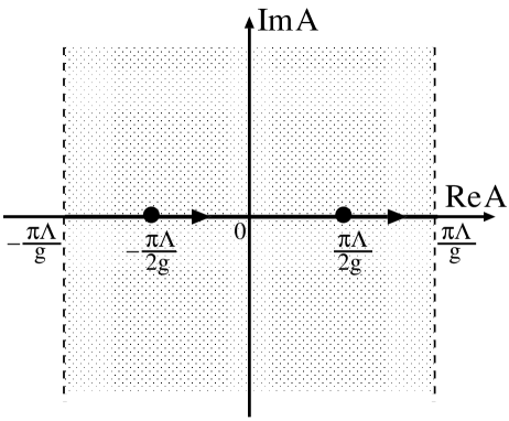
Figure 2: The target space of the scalar field $A$. The lines at ${\rm Re}A=\pm\pi\Lambda/g$ are identified with each other. The SUSY vacua are $A=\pm\pi\Lambda/(2g)$.

There are BPS and anti-BPS walls interpolating these two vacua. The BPS wall solution is

$$A_{\rm cl1}(x_{2})=\frac{\Lambda}{g}\left\{2\tan^{-1}e^{\Lambda x_{2}}-\frac{\pi}{2}\right\},$$ (101)

which interpolates from the vacuum at $A_{\rm I}=-\frac{\pi\Lambda}{2g}$ to the one at $A_{\rm II}=\frac{\pi\Lambda}{2g}$ as $y$ increases from $y=-\infty$ to $y=\infty$. The anti-BPS wall solution is

$$A_{\rm cl2}(x_{2})=\frac{\Lambda}{g}\left\{-2\tan^{-1}e^{-\Lambda x_{2}}+\frac{3\pi}{2}\right\},$$ (102)

which interpolates from $A_{\rm II}=\frac{\pi\Lambda}{2g}$ to $A_{\rm I}=\frac{3\pi\Lambda}{2g}(=-\frac{\pi\Lambda}{2g})$. Thus, a field configuration corresponding to the coexistence of these walls will wrap around the cylinder of the target space of $A$ as $x_{2}$ goes around $S^{1}$. Such a topological winding ensures the stability of the configuration.

Indeed, there is a solution of the equation of motion,

$$\partial^{\mu}\partial_{\mu}A+\frac{\Lambda^{3}}{g}\sin\left(\frac{g}{\Lambda}\bar{A}\right)\cos\left(\frac{g}{\Lambda}A\right)=0,$$ (103)

which corresponds to the wall-antiwall system. That is,

$$A_{\rm cl}(x_{2})=\frac{\Lambda}{g}{\rm am}\left(\frac{\Lambda}{k}x_{2},k\right),$$ (104)

where $k$ is a real parameter and the function ${\rm am}(u,k)$ denotes the amplitude function, which is defined as an inverse function of

$$u(\varphi)=\int_{0}^{\varphi}\>\frac{{\rm d}\theta}{\sqrt{1-k^{2}\sin^{2}\theta}}.$$ (105)

For $k<1$, $A_{\rm cl}(x_{2})$ is a monotonically increasing function, and has a desired topological winding number. The parameter $k$ is related to the radius of the compact space $R$ through

$$2\pi R=\frac{4k}{\Lambda}K(k),$$ (106)

where $K(k)$ is the complete elliptic integral of the first kind. In the case of $2\pi R\Lambda\gg 1$, in other words, when the configuration $A_{\rm cl}(x_{2})$ can be regarded as a wall-antiwall system, the parameter $k$ is close to one, and can approximately be written as

$$k\simeq\sqrt{1-16e^{-\pi R\Lambda}}.$$ (107)

A profile of $A_{\rm cl}(x_{2})$ is shown in Fig.3.

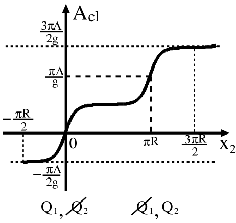
Figure 3: The profile of the classical solution $A_{\rm cl}(x_{2})$. The dotted lines $A=-\pi\Lambda/(2g)$ and $A=3\pi\Lambda/(2g)$ are identified.

Solving the mode equation (31) for this background, we can obtain the normalized mode functions of the zero-modes as follows.

$$u_{{\rm R}(0)}(x_{2})\!\!\! =\!\!\! \frac{\Lambda^{2}}{gk\sqrt{V_{0}}}\left\{{\rm dn}\left(\frac{\Lambda}{k}x_{2},k\right)+k{\rm cn}\left(\frac{\Lambda}{k}x_{2},k\right)\right\},$$

$$u_{{\rm I}(0)}(x_{2})\!\!\! =\!\!\! \frac{\Lambda^{2}}{gk\sqrt{V_{0}}}\left\{{\rm dn}\left(\frac{\Lambda}{k}x_{2},k\right)-k{\rm cn}\left(\frac{\Lambda}{k}x_{2},k\right)\right\},$$ (108)

where functions ${\rm cn}(u,k)$ and ${\rm dn}(u,k)$ are the Jacobi’s elliptic functions. The profiles of these mode-functions are shown in Fig.4. With these expressions, we can calculate all parameters of the 3D effective theory by using the formulae (40), (65) and (66).

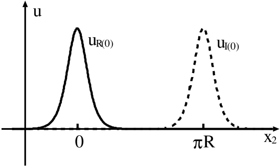
Figure 4: The profiles of the mode-functions $u_{{\rm R}(0)}(x_{2})$ and $u_{{\rm I}(0)}(x_{2})$.

As discussed in Sect.3.4, we can introduce matter fields localized on the walls. Let us introduce a matter chiral superfield $X$ in the 4D bulk theory, and assume an interaction to the “wall superfield” $\Phi$ as

$$W_{\rm int}(\Phi,X)=\frac{\alpha}{2}W^{\prime\prime}(\Phi)X^{2}=-\frac{\alpha}{2}\Lambda\sin\left(\frac{g}{\Lambda}\Phi\right)X^{2},$$ (109)

where a dimensionless constant $\alpha$ is positive.

The field configuration

$$A_{\rm cl}(x_{2})\!\!\! =\!\!\! \frac{\Lambda}{g}{\rm am}\left(\frac{\Lambda}{k}x_{2},k\right),$$

$$A_{X{\rm cl}}(x_{2})\!\!\! =\!\!\! 0,$$ (110)

is a static solution of the equation of motion. Solving the mode equations (71) for this background, we can obtain the mode functions of the zero-modes for the matter fields as follows.

$$u_{{\rm R}X(0)}(x_{2})\!\!\! =\!\!\! C_{X}\left\{{\rm dn}\left(\frac{\Lambda}{k}x_{2},k\right)+k{\rm cn}\left(\frac{\Lambda}{k}x_{2},k\right)\right\}^{\alpha},$$

$$u_{{\rm I}X(0)}(x_{2}))\!\!\! =\!\!\! C_{X}\left\{{\rm dn}\left(\frac{\Lambda}{k}x_{2},k\right)-k{\rm cn}\left(\frac{\Lambda}{k}x_{2},k\right)\right\}^{\alpha},$$ (111)

where $C_{X}$ is a common normalization factor. Then, the 3D effective theory in this case is

$${\cal L}^{(3)}\!\!\! =\!\!\! -V_{0}+\int\!\!{\rm d}^{2}\theta_{1}\>\left\{\frac{1}{2}(D_{1}\varphi^{(1)}_{(0)})^{2}+\frac{1}{2}(D_{1}\varphi^{(1)}_{X(0)})^{2}\right\}+\int\!\!{\rm d}^{2}\theta_{2}\>\left\{\frac{1}{2}(D_{2}\varphi^{(2)}_{(0)})^{2}+\frac{1}{2}(D_{2}\varphi^{(2)}_{X(0)})^{2}\right\}$$ (112)

$$-\eta\left(f^{(1)}_{(0)}f^{(2)}_{(0)}+\partial^{m}a^{(1)}_{(0)}\partial_{m}a^{(2)}_{(0)}\right)-\eta_{X}\left(f^{(1)}_{X(0)}f^{(2)}_{X(0)}+\partial^{m}a^{(1)}_{X(0)}\partial_{m}a^{(2)}_{X(0)}\right)$$

$$-\frac{1}{2}m_{0}^{2}\left(a^{(1)}_{(0)}-a^{(2)}_{(0)}\right)^{2}-\frac{1}{2}m_{X}^{2}\left((a^{(1)}_{X(0)})^{2}+(a^{(2)}_{X(0)})^{2}\right)-\Delta m_{X}^{2}a^{(1)}_{X(0)}a^{(2)}_{X(0)}$$

$$+\mbox{(interaction terms)},$$

where

$$m_{0}^{2}\!\!\! =\!\!\! \frac{1-k^{2}}{2k^{2}}\Lambda^{2}\left(1-\frac{2(1-k^{2})}{g^{2}k^{2}V_{0}}\Lambda^{4}\pi R\right),$$

$$m_{X}^{2}\!\!\! =\!\!\! \alpha\frac{\Lambda^{2}}{k}C_{X}^{2}(1-k^{2})\int\!\!{\rm d}x_{2}\>{\rm cn}\left(\frac{\Lambda}{k}x_{2},k\right)\left\{{\rm dn}\left(\frac{\Lambda}{k}x_{2},k\right)+k{\rm cn}\left(\frac{\Lambda}{k}x_{2},k\right)\right\}^{2\alpha-1},$$

$$\Delta m_{X}^{2}\!\!\! =\!\!\! \alpha\Lambda^{2}C_{X}^{2}(1-k^{2})^{\alpha}\left(\frac{g^{2}V_{0}}{2\Lambda^{4}}-\frac{1-k^{2}}{k^{2}}\pi R\right),$$

$$\eta\!\!\! =\!\!\! \frac{2\pi R}{V_{0}}\frac{\Lambda^{4}}{g^{2}k^{2}}(1-k^{2}),\;\;\;\;\;\;\;\eta_{X}=2\pi RC_{X}^{2}(1-k^{2})^{\alpha}.$$ (113)

From these expressions, we can obtain the mass eigenvalue of $a_{-(0)}$ defined in Eq.(59) as

$$\frac{2m_{0}^{2}}{1-\eta}=\frac{1-k^{2}}{k^{2}}\Lambda^{2}.$$ (114)

This coincides with the result of Ref.[15].

Fig.5 shows the ratio $m_{X}^{2}/\Delta m_{X}^{2}$ as a function of $\alpha$. From this plot, we can see that $m_{X}^{2}<|\Delta m_{X}^{2}|$ in the region of $0<\alpha<1$. This means that a tachyonic mode appears in the effective theory, and the classical background (110) is not stable in this region.

Figure 5: The ratio $m_{X}^{2}/\Delta m_{X}^{2}$ as a function of $\alpha$.

In the case of $\alpha>1$, the background is stable since $m_{X}^{2}>|\Delta m_{X}^{2}|$. Here, note that $\alpha$ itself is not the coupling constant between $\Phi$ and $X$. Indeed, $W_{\rm int}$ in Eq.(109) is expanded as

$$W_{\rm int}(\Phi,X)=-\frac{\alpha g}{2}\Phi X^{2}+\cdots,$$ (115)

where ellipsis denotes higher dimensional operators suppressed by the scale $\Lambda$. Thus, the true coupling constant is $\alpha g/2$. Therefore, the large value of $\alpha$ does not represent the strong coupling region as long as $\alpha g/2$ is small.

In this model, an exact solution (104) is known. In general, however, it is not easy to find such a non-BPS solution because we must solve a second order differential equation. On the other hand, BPS wall solutions can easily be found at least numerically since the BPS equation is a first order differential equation. As we explained in the previous section, we can calculate the parameters of the 3D effective theory with high accuracy by using only the BPS wall solutions $A_{\rm cl1}(x_{2})$ and $A_{\rm cl2}(x_{2})$. For example, an approximate expression of $U_{{\rm I}0}(x_{2})$ can be obtained from Eq.(96) as

$$U_{{\rm I}0}(x_{2})\simeq\left\{\parbox{170.71652pt}{\begin{displaymath}\frac{2\Lambda^{2}}{g}\frac{\cosh(\Lambda x_{2})}{\cosh^{2}(\pi R\Lambda/2)}\;\;\;\left(-\frac{\pi R}{2}<x_{2}\leq\frac{\pi R}{2}\right)\end{displaymath} \begin{displaymath}\frac{2\Lambda^{2}}{g}\frac{1}{\cosh\left\{\Lambda(x_{2}-\pi R)\right\}}\;\;\;\left(\frac{\pi R}{2}<x_{2}\leq\frac{3\pi R}{2}\right)\end{displaymath}}\right.$$ (116)

$U_{{\rm R}0}(x_{2})$ and the mode functions can also be approximated in a similar way.

6 Interaction with the gauge supermultiplet

In this section, we will derive the 3D effective theory including a gauge supermultiplet. For simplicity, we will discuss an abelian gauge theory. An extension to the non-abelian case is straightforward. Let us introduce a vector superfield $V(x^{\mu},\theta,\bar{\theta})$ in the 4D bulk theory. In the Wess-Zumino gauge, its component fields are denoted as

$$V(x^{\mu},\theta,\bar{\theta})=-\theta\sigma^{\mu}\bar{\theta}v_{\mu}+i\theta^{2}\bar{\theta}\bar{\lambda}-i\bar{\theta}^{2}\theta\lambda+\frac{1}{2}\theta^{2}\bar{\theta}^{2}D.$$ (117)

When we consider interactions with fields localized on the BPS wall $A_{\rm cl1}(x_{2})$, it is useful to expand $V(x^{\mu},\theta,\bar{\theta})$ as [18]

$$V(x^{\mu},\theta,\bar{\theta})=e^{-\theta_{1}\theta_{2}\partial_{2}}\left\{\theta_{2}\rho^{(1)}(x^{m},x_{2},\theta_{1})+\theta_{2}^{2}\sigma^{(1)}(x^{m},x_{2},\theta_{1})\right\},$$ (118)

where

$$\rho^{(1)}_{\alpha}(x^{m},x_{2},\theta_{1})\!\!\! \equiv\!\!\! -i\left(\gamma_{(3)}^{m}\theta_{1}\right)_{\alpha}v_{m}-\theta_{1}^{2}\lambda_{1\alpha},$$

$$\sigma^{(1)}(x^{m},x_{2},\theta_{1})\!\!\! \equiv\!\!\! -v_{2}-\theta_{1}\lambda_{2}-\frac{1}{2}\theta_{1}^{2}D.$$ (119)

Here, 3D Majorana-like spinors $\lambda_{1}$ and $\lambda_{2}$, which still have the $x_{2}$-dependence, are defined by the decomposition,

$$\lambda^{\alpha}=\frac{e^{i\delta/2}}{\sqrt{2}}(\lambda_{2}^{\alpha}+i\lambda_{1}^{\alpha}).$$ (120)

Using the 4D gauge transformation, we can eliminate the 3D scalar $v_{2}$ except for its zero-mode $v_{2(0)}$ [18].

In this case, the 4D superfield strength $W_{\alpha}\equiv-\frac{1}{4}\bar{D}^{2}D_{\alpha}V$ can be written as

$$W_{\alpha}(y^{\mu},\theta)=-\frac{i}{\sqrt{2}}e^{i\delta/2}e^{-\theta_{1}\theta_{2}\partial_{2}}e^{-i\theta_{2}D_{1}+i\theta_{2}^{2}\partial_{2}}\left\{u^{(1)}_{\alpha}(x^{m},x_{2},\theta_{1})+iw^{(1)}_{\alpha}(x^{m},x_{2},\theta_{1})\right\},$$ (121)

where $u^{(1)}_{\alpha}$ and $w^{(1)}_{\alpha}$ are 3D gauge invariant quantities and defined as

$$u^{(1)}_{\alpha}(x^{m},x_{2},\theta_{1})\!\!\! \equiv\!\!\! e^{\theta_{1}Q_{1}}\times\lambda_{2\alpha}=D_{1\alpha}\sigma^{(1)}+\partial_{2}\rho^{(1)}_{\alpha}$$

$$=\!\!\! \lambda_{2\alpha}-\theta_{1\alpha}D+i\left(\gamma_{(3)}^{m}\theta_{1}\right)_{\alpha}v_{m2}+\theta_{1}^{2}\left\{\frac{i}{2}\left(\gamma_{(3)}^{m}\partial_{m}\lambda_{2}\right)_{\alpha}-\partial_{2}\lambda_{1\alpha}\right\},$$

$$w^{(1)}_{\alpha}(x^{m},x_{2},\theta_{1})\!\!\! \equiv\!\!\! e^{\theta_{1}Q_{1}}\times\lambda_{1\alpha}=\frac{1}{4}D_{1}^{2}\rho^{(1)}_{\alpha}+\frac{i}{2}\left(\gamma_{(3)}^{m}\partial_{m}\rho^{(1)}\right)_{\alpha}$$ (122)

$$=\!\!\! \lambda_{1\alpha}+\left(\gamma_{(3)}^{mn}\theta_{1}\right)_{\alpha}v_{mn}-\frac{i}{2}\theta_{1}^{2}\left(\gamma_{(3)}^{m}\partial_{m}\lambda_{1}\right)_{\alpha}.$$

Here, $v_{\mu\nu}\equiv\partial_{\mu}v_{\nu}-\partial_{\nu}v_{\mu}$ is a 4D field strength.

Similarly, when we consider interactions with fields localized on the anti-BPS wall $A_{\rm cl2}(x_{2})$, the following expansion is useful.

$$V(x^{\mu},\theta,\bar{\theta})=e^{\theta_{1}\theta_{2}\partial_{2}}\left\{-\theta_{1}\rho^{(2)}(x^{m},x_{2},\theta_{2})+\theta_{1}^{2}\sigma^{(2)}(x^{m},x_{2},\theta_{2})\right\},$$ (123)

where

$$\rho^{(2)}_{\alpha}(x^{m},x_{2},\theta_{2})\!\!\! \equiv\!\!\! -i\left(\gamma_{(3)}^{m}\theta_{2}\right)_{\alpha}v_{m}-\theta_{2}^{2}\lambda_{2\alpha},$$

$$\sigma^{(2)}(x^{m},x_{2},\theta_{2})\!\!\! \equiv\!\!\! -v_{2}-\theta_{2}\lambda_{1}-\frac{1}{2}\theta_{2}^{2}D.$$ (124)

In this case, $W_{\alpha}$ can be written as

$$W_{\alpha}(y^{\mu},\theta)=-\frac{i}{\sqrt{2}}e^{i\delta/2}e^{\theta_{1}\theta_{2}\partial_{2}}e^{i\theta_{1}D_{2}+i\theta_{1}^{2}\partial_{2}}\left\{u^{(2)}_{\alpha}(x^{m},x_{2},\theta_{2})-iw^{(2)}_{\alpha}(x^{m},x_{2},\theta_{2})\right\},$$ (125)

where $u^{(2)}_{\alpha}$ and $w^{(2)}_{\alpha}$ are another 3D gauge invariant quantities, and defined as

$$u^{(2)}_{\alpha}(x^{m},x_{2},\theta_{2})\!\!\! \equiv\!\!\! e^{\theta_{2}Q_{2}}\times\lambda_{1\alpha}=-D_{2\alpha}\sigma^{(2)}-\partial_{2}\rho^{(2)}_{\alpha}$$

$$=\!\!\! \lambda_{1\alpha}+\theta_{2\alpha}D-i\left(\gamma_{(3)}^{m}\theta_{2}\right)_{\alpha}v_{m2}+\theta_{2}^{2}\left\{\frac{i}{2}\left(\gamma_{(3)}^{m}\partial_{m}\lambda_{1}\right)_{\alpha}+\partial_{2}\lambda_{2\alpha}\right\},$$

$$w^{(2)}_{\alpha}(x^{m},x_{2},\theta_{2})\!\!\! \equiv\!\!\! e^{\theta_{2}Q_{2}}\times\lambda_{2\alpha}=\frac{1}{4}D_{2}^{2}\rho^{(2)}_{\alpha}+\frac{i}{2}\left(\gamma_{(3)}^{m}\partial_{m}\rho^{(2)}\right)_{\alpha}$$ (126)

$$=\!\!\! \lambda_{2\alpha}+\left(\gamma_{(3)}^{mn}\theta_{2}\right)_{\alpha}v_{mn}-\frac{i}{2}\theta_{2}^{2}\left(\gamma_{(3)}^{m}\partial_{m}\lambda_{2}\right)_{\alpha}.$$

The kinetic terms for the gauge supermultiplet can be rewritten in terms of $u^{(1)}_{\alpha}$ and $w^{(1)}_{\alpha}$, i.e. $\rho^{(1)}_{\alpha}$ and $\sigma^{(1)}$, as

$$S^{V}_{\rm kin}\!\!\! =\!\!\! \int\!\!{\rm d}^{4}x{\rm d}^{2}\theta\>\frac{1}{4}W^{\alpha}W_{\alpha}+{\rm h.c.}$$ (127)

$$=\!\!\! \int\!\!{\rm d}^{3}x{\rm d}^{2}\theta_{1}\>\frac{1}{2}\left\{(u^{(1)})^{2}-(w^{(1)})^{2}\right\}.$$

Here we have assumed a minimal gauge kinetic function, for simplicity.

Similarly, Eq.(127) can also be rewritten in terms of $u^{(2)}_{\alpha}$ and $w^{(2)}_{\alpha}$, i.e. $\rho^{(2)}_{\alpha}$ and $\sigma^{(2)}$, as

$$S^{V}_{\rm kin}=\int\!\!{\rm d}^{3}x{\rm d}^{2}\theta_{2}\>\frac{1}{2}\left\{(u^{(2)})^{2}-(w^{(2)})^{2}\right\}.$$ (128)

In this case, the mode-expansion of the gauge supermultiplet is trivial. That is,

$$\rho^{(1)\alpha}(x^{m},x_{2},\theta_{1})\!\!\! =\!\!\! \frac{1}{\sqrt{2\pi R}}\rho^{(1)\alpha}_{(0)}(x^{m},\theta_{1})$$

$$+\sum_{n=1}^{\infty}\frac{1}{\sqrt{\pi R}}\left\{\cos\frac{nx_{2}}{R}\cdot\rho^{(1)\alpha}_{(n+)}(x^{m},\theta_{1})+\sin\frac{nx_{2}}{R}\cdot\rho^{(1)\alpha}_{(n-)}(x^{m},\theta_{1})\right\},$$

$$\sigma^{(1)}(x^{m},x_{2},\theta_{1})\!\!\! =\!\!\! \frac{1}{\sqrt{2\pi R}}\sigma^{(1)}_{(0)}(x^{m},\theta_{1})$$

$$+\sum_{n=1}^{\infty}\frac{1}{\sqrt{\pi R}}\left\{\cos\frac{nx_{2}}{R}\cdot\sigma^{(1)}_{(n+)}(x^{m},\theta_{1})+\sin\frac{nx_{2}}{R}\cdot\sigma^{(1)}_{(n-)}(x^{m},\theta_{1})\right\}.$$

The mode-expansions of $\rho^{(2)\alpha}$ and $\sigma^{(2)}$ can be done in a similar way.

Next, we will consider the gauge interaction with the matter field $X$. In the 4D bulk theory, it is written as

$$S_{\rm matter}^{V}=\int\!\!{\rm d}^{4}x{\rm d}^{2}\theta{\rm d}^{2}\bar{\theta}\>\bar{X}e^{2qV}X,$$ (130)

where $q$ is a gauge coupling constant.

Notice that the abelian gauge symmetry should be represented as an $SO(2)$ symmetry in our case since 3D superfields are real. Thus, the vector superfield $V$ discussed so far should be understood as a $2\times 2$ matrix,

$$V=V_{\rm R}\left(\begin{array}[]{cc}0&-i\\ i&0\end{array}\right),$$ (131)

where $V_{\rm R}$ is a real vector superfield. The matter superfield $X$ should be understood as a 2-component column vector whose gauge transformation is

$$X\to\exp\left\{-2q\Lambda\left(\begin{array}[]{cc}0&-i\\ i&0\end{array}\right)\right\}X,$$ (132)

where $\Lambda$ is a transformation parameter, which is a chiral superfield.

Then, by substituting Eqs.(9) and (118) into Eq.(130) and carrying out the $\theta_{2}$-integration, the following expression can be obtained.

$$S_{\rm matter}^{V}\!\!\! =\!\!\! \int\!\!{\rm d}^{3}x{\rm d}^{2}\theta_{1}{\rm d}x_{2}\>\left\{D_{1}^{\alpha}\bar{\varphi}^{(1)}_{X}D_{1\alpha}\varphi^{(1)}_{X}+2{\rm Im}\left(\bar{\varphi}^{(1)}_{X}\partial_{2}\varphi^{(1)}_{X}\right)+2q{\rm Im}\left(\bar{\varphi}^{(1)}_{X}\rho^{(1)}D_{1}\varphi^{(1)}_{X}\right)\right.$$ (133)

$$\hskip 76.82234pt\left.-\bar{\varphi}^{(1)}(2q\sigma^{(1)}-q^{2}\rho^{(1)2})\varphi^{(1)}\right\}.$$

In order to derive the 3D effective theory, we should substitute mode-expansions (74) and (LABEL:rhsg_mode_ex) into the above expression. Note that there are a lot of light modes in the gauge supermultiplet when the compactified radius $R$ is large compared to the wall width. They will remain to be the dynamical degrees of freedom after the massive matter modes are integrated out.

As a result, the interaction terms with the gauge supermultiplet can be obtained as follows.

$${\cal L}^{(3)}_{\rm int}\!\!\! =\!\!\! \int\!\!{\rm d}^{2}\theta_{1}\>\left[q_{(0)}{\rm Im}\left({}^{t}\varphi^{(1)}_{X(0)}\rho^{(1)}_{(0)}D_{1}\varphi^{(1)}_{X(0)}\right)+\frac{1}{2}q_{(0)}^{2}{}^{t}\varphi^{(1)}_{X(0)}\rho^{(1)2}_{(0)}\varphi^{(1)}_{X(0)}\right.$$ (134)

$$\hskip 42.67912pt+\sum_{l=1}^{\infty}\sum_{s=\pm}q_{(ls)}\left\{{\rm Im}\left({}^{t}\varphi^{(1)}_{X(0)}\rho^{(1)}_{(ls)}D_{1}\varphi^{(1)}_{X(0)}\right)+q_{(0)}{}^{t}\varphi^{(1)}_{X(0)}\rho^{(1)}_{(ls)}\rho^{(1)}_{(0)}\varphi^{(1)}_{X(0)}\right\}$$

$$\hskip 42.67912pt\left.+\frac{1}{2}\sum_{l,p=1}^{\infty}\sum_{s,t=\pm}\left(q^{2}\right)_{(ls,pt)}{}^{t}\varphi^{(1)}_{X(0)}\rho^{(1)}_{(ls)}\rho^{(1)}_{(pt)}\varphi^{(1)}_{X(0)}\right]$$

$$+\int\!\!{\rm d}^{2}\theta_{2}\>\left[q_{(0)}{\rm Im}\left({}^{t}\varphi^{(2)}_{X(0)}\rho^{(2)}_{(0)}D_{2}\varphi^{(2)}_{X(0)}\right)+\frac{1}{2}q_{(0)}^{2}{}^{t}\varphi^{(2)}_{X(0)}\rho^{(2)2}_{(0)}\varphi^{(2)}_{X(0)}\right.$$

$$\hskip 51.21495pt+\sum_{l=1}^{\infty}\sum_{s=\pm}q_{(ls)}\left\{{\rm Im}\left({}^{t}\varphi^{(2)}_{X(0)}\rho^{(2)}_{(ls)}D_{2}\varphi^{(2)}_{X(0)}\right)+q_{(0)}{}^{t}\varphi^{(2)}_{X(0)}\rho^{(2)}_{(ls)}\rho^{(2)}_{(0)}\varphi^{(2)}_{X(0)}\right\}$$

$$\hskip 51.21495pt\left.+\frac{1}{2}\sum_{l,p=1}^{\infty}\sum_{s,t=\pm}\left(q^{2}\right)_{(ls,pt)}{}^{t}\varphi^{(2)}_{X(0)}\rho^{(2)}_{(ls)}\rho^{(2)}_{(pt)}\varphi^{(2)}_{X(0)}\right]$$

$$+{\cal L}^{(3)}_{{\rm SUSY}\begin{picture}(10.0,5.0)\line(4,1){23.0}\end{picture}}\hskip 11.38109pt,$$

where $q_{(0)}\equiv q/\sqrt{2\pi R}$ is the 3D gauge coupling constant, and the other effective couplings are defined as

$$q_{(n+)}\!\!\! \equiv\!\!\! \frac{g}{\sqrt{\pi R}}\int\!\!{\rm d}x_{2}\>u_{{\rm R}X(0)}^{2}\cos\frac{nx_{2}}{R}=\frac{g}{\sqrt{\pi R}}\int\!\!{\rm d}x_{2}\>u_{{\rm I}X(0)}^{2}\cos\frac{n(x_{2}-\pi R)}{R},$$

$$q_{(n-)}\!\!\! \equiv\!\!\! \frac{g}{\sqrt{\pi R}}\int\!\!{\rm d}x_{2}\>u_{{\rm R}X(0)}^{2}\sin\frac{nx_{2}}{R}=\frac{g}{\sqrt{\pi R}}\int\!\!{\rm d}x_{2}\>u_{{\rm I}X(0)}^{2}\sin\frac{n(x_{2}-\pi R)}{R},$$

$$\left(q^{2}\right)_{(n+,m+)}\!\!\! \equiv\!\!\! \frac{g^{2}}{\pi R}\int\!\!{\rm d}x_{2}\>u_{{\rm R}X(0)}^{2}\cos\frac{nx_{2}}{R}\cos\frac{mx_{2}}{R},$$

$$\left(q^{2}\right)_{(n+,m-)}\!\!\! \equiv\!\!\! \frac{g^{2}}{\pi R}\int\!\!{\rm d}x_{2}\>u_{{\rm R}X(0)}^{2}\cos\frac{nx_{2}}{R}\sin\frac{mx_{2}}{R},$$ (135)

$$\vdots$$

and ${\cal L}^{(3)}_{{\rm SUSY}\begin{picture}(10.0,5.0)\line(4,1){23.0}\end{picture}}$     denotes the SUSY breaking terms as follows.

$${\cal L}^{(3)}_{{\rm SUSY}\begin{picture}(10.0,5.0)\line(4,1){23.0}\end{picture}}\hskip 11.38109pt\!\!\! =\!\!\! -\eta_{X}{}^{t}\!\left(\partial^{m}a^{(1)}_{X(0)}+iq_{(0)}v_{(0)}^{m}a^{(1)}_{X(0)}\right)\left(\partial_{m}a^{(2)}_{X(0)}+iq_{(0)}v_{(0)m}a^{(2)}_{X(0)}\right)$$ (136)

$$+i\eta_{X}q_{(0)}\left(a^{(1)}_{X(0)}\lambda_{1(0)}\psi_{{\rm I}X(0)}+a^{(2)}_{X(0)}\lambda_{2(0)}\psi_{{\rm R}X(0)}\right)-i\eta_{X}q_{(0)}\psi_{{\rm R}X(0)}v_{2(0)}\psi_{{\rm I}X(0)}$$

$$+\cdots,$$

where ellipsis denotes terms involving the Kaluza-Klein modes for the gauge supermultiplet.

The gaugino mass terms are induced at loop-level in this model.

7 Summary and discussion

We have provided a useful method for the derivation of the effective theory in a system where BPS and anti-BPS domain walls coexist. Although the corresponding field configuration $A_{\rm cl}(x_{2})$ is non-BPS, it can approximately be regarded as a BPS wall or an anti-BPS wall in the neighborhood of each domain wall. So the light modes localized on one of the walls form (approximate) supermultiplets for the corresponding 3D ${\cal N}=1$ SUSY. Due to the existence of the other wall, however, such approximate SUSYs are broken. Thus, the 3D effective theory for this system consists of two parts; a supersymmetric part described by 3D superfields and a SUSY breaking part. All parameters of the effective theory can be calculated systematically in our method.

The SUSY breaking terms can be classified into two types. The first-type ones involve only modes localized on the same wall. Such terms are induced due to the deviation of the background from the BPS wall, which is mainly characterized by $U_{{\rm R}0}(x_{2})$ or $U_{{\rm I}0}(x_{2})$ in Eq.(42). Indeed, all parameters for such terms are expressed by overlap integrals involving $U_{{\rm R}0}(x_{2})$ or $U_{{\rm I}0}(x_{2})$. The second-type ones are direct couplings between modes localized on the different walls. Both types of the SUSY breaking terms receive an exponential suppression in terms of the ratio of the wall distance $\pi R$ to the wall width $\lambda_{w}$. In particular, all SUSY breaking terms vanish at tree-level in the “thin-wall” limit, i.e. $\pi R/\lambda_{w}\to\infty$. This situation corresponds to the pseudo-supersymmetry discussed in Ref.[12]. In this limit, SUSY breaking is induced through the loop effects involving the bulk fields, such as the gauge field discussed in Sect.6. In the case that $\pi R/\lambda_{w}$ is finite, on the other hand, the tree-level terms of SUSY breaking discussed in this paper arise besides the loop-induced ones. It depends on the ratio $\pi R/\lambda_{w}$ whether the tree-level ones dominate over the loop-induced ones or not.

From the SUSY breaking mass terms calculated in our method, we have shown that maximal mixings occur between the bosonic zero-modes localized on the different walls, while the fermionic zero-modes remain to be localized on each wall. This means that oscillations will occur between the bosonic modes localized on the different walls.

An effective theory on the domain wall can also be derived by using the nonlinear realization technique for the space-time symmetries. In particular, we can obtain an effective theory on a BPS wall by regarding the existence of the wall as the partial SUSY breaking [25]. This method is powerful for the general discussion of the BPS walls because it uses only information on symmetries. The relation between this method and the mode-expansion method [26, 18] is discussed in Ref.[27]. Similarly, we can derive an effective theory on a non-BPS wall by the nonlinear realization method [28]. Since the wall-antiwall system is non-BPS, we can apply this method to our case. However, the nonlinear realization method cannot respect a specific structure of the configuration, such as the wall-antiwall structure. Thus, in order to discuss the specific features of the wall-antiwall system, we have to take the mode-expansion method as we have done in this paper. If you would like to know the relation between our result and the result of Ref.[28], you should combine our method with the result of Ref.[27].

In this paper, we have concentrated ourselves on the case that the Kähler potential is minimal, for simplicity. An extension to the non-minimal Kähler case is possible, although the classical background $A_{\rm cl}(x_{2})$ and the mode functions cannot be obtained analytically in that case. Thus, the BPS-wall approximation discussed in Sect.4 is useful in such a case because solving the BPS equations (the first order differential equations) is much easier than solving the equations of motion (the second order differential equations) in the numerical calculation.

When we introduce the matter fields, we must take care of the strength of the couplings between the matter and the wall fields. As we have demonstrated in Sect.5, a weak coupling between them leads to a tachyonic scalar mode in the effective theory. This means that the background field configuration is unstable unless the matter modes are strongly localized on the walls. Roughly speaking, if the matter modes are localized within the wall width $\lambda_{w}$, the background is stable. Therefore, the fat brane scenario [5, 7] is allowed in the wall-antiwall system. Using the above tachyonic mode as the “Higgs” field, it might be possible to propose a new mechanism of symmetry breaking.

In the superstring theory, it is well-known that BPS D-branes can be described by the kink solutions in the tachyon field theory [21]. In particular, a system where D$p$ brane and anti-D$p$ brane coexist is represented by a wall-antiwall solution in an effective field theory on a non-BPS D$(p+1)$-brane [22]. Thus, our method discussed here is useful in the discussion of the tachyon condensation [23] in the superstring theory.

In order to construct a more realistic model, we have to investigate a wall-antiwall system in a 5D SUSY theory. However, 5D SUSY theories are difficult to handle because they have many SUSY (at least eight supercharges). In fact, 5D SUSY theories are required to be nonlinear sigma models in order to have a BPS domain wall [29], due to their restrictive forms of the scalar potential. However, our approach suggests how to derive the 4D effective theory for the wall-antiwall system, once we find a method for deriving an effective theory on a BPS wall in five dimensions. Expanding the discussion to the supergravity is also an interesting subject.

Acknowledgments

The author thanks Nobuhito Maru, Norisuke Sakai and Ryo Sugisaka for a collaboration of previous works which motivate this work. The author also thanks the Yukawa Institute for Theoretical Physics at Kyoto University, where this work was initiated during the YITP-W-02-04 on “Quantum Field Theory 2002”.

Appendix A Notations

Basically, we follow the notations of Ref.[30] for the 4D bulk theory.

A.1 Notations for 3D theories

The notations for the 3D theories are as follows.

We take the space-time metric as

$$\eta^{mn}={\rm diag}(-1,+1,+1).$$ (137)

The 3D $\gamma$-matrices, $(\gamma_{(3)}^{m})_{\alpha}^{\;\beta}$, can be written by the Pauli matrices as

$$\gamma_{(3)}^{0}=\sigma^{2},\;\;\;\gamma_{(3)}^{1}=-i\sigma^{3},\;\;\;\gamma_{(3)}^{3}=i\sigma^{1},$$ (138)

and these satisfy the 3D Clifford algebra,

$$\left\{\gamma_{(3)}^{m},\gamma_{(3)}^{n}\right\}=-2\eta^{mn}.$$ (139)

The spinor indices are raised and lowered by multiplying $\sigma^{2}$ from the left.

$$\psi_{\alpha}=\left(\sigma^{2}\right)_{\alpha\beta}\psi^{\beta},\;\;\;\psi^{\alpha}=\left(\sigma^{2}\right)^{\alpha\beta}\psi_{\beta}.$$ (140)

We take the following convention of the contraction of spinor indices.

$$\psi_{1}\psi_{2}\equiv\psi_{1}^{\alpha}\psi_{2\alpha}=\left(\sigma^{2}\right)_{\alpha\beta}\psi_{1}^{\alpha}\psi_{2}^{\beta}=\psi_{2}\psi_{1}.$$ (141)

Appendix B Properties of $A_{\rm cl}(x_{2})$

Here, we collect some properties of the classical configuration $A_{\rm cl}(x_{2})$.

The equation of motion for the classical solution $A_{\rm cl}(x_{2})$ is

$$\partial_{2}^{2}A_{\rm cl}-W^{\prime}(A_{\rm cl})\bar{W}^{\prime\prime}(\bar{A}_{\rm cl})=0.$$ (142)

By multiplying $\partial_{2}\bar{A}_{\rm cl}(x_{2})$ with this equation, we will obtain

$$\frac{1}{2}\partial_{2}\left\{|\partial_{2}A_{\rm cl}|^{2}-|W^{\prime}(A_{\rm cl})|^{2}\right\}=0.$$ (143)

This means that

$$|\partial_{2}A_{\rm cl}|^{2}-|W^{\prime}(A_{\rm cl})|^{2}=c,$$ (144)

where $c$ is a real constant. In the case that $A_{\rm cl}(x_{2})$ is a BPS wall configuration, we can see that $c=0$ from the BPS equation. For the wall-antiwall configuration, $c$ is a tiny constant. Typically, it is exponentially suppressed by the wall distance $\pi R$. In the model discussed in Sect.5, for instance,

$$c=\left(\frac{\Lambda^{2}}{gk}\right)^{2}(1-k^{2})\simeq 16\frac{\Lambda^{4}}{g^{2}}e^{-\pi R\Lambda}.$$ (145)

In particular, in the case of the real configuration mainly discussed in this paper, Eq.(144) can be rewritten as

$$U_{{\rm R}0}(x_{2})U_{{\rm I}0}(x_{2})=V_{0}u_{{\rm R}(0)}(x_{2})u_{{\rm I}(0)}(x_{2})=c.$$ (146)

Thus, $c$ is related to $\eta$ in Eq.(39) through

$$c=\frac{V_{0}}{2\pi R}\eta.$$ (147)

Under the assumption (21), the following relations hold.

$$W^{\prime\prime}(A_{\rm cl}(x_{2}-\pi R))\!\!\! =\!\!\! -W^{\prime\prime}(A_{\rm cl}(x_{2})),$$

$$W^{\prime\prime}(A_{\rm cl}(-x_{2}))\!\!\! =\!\!\! W^{\prime\prime}(A_{\rm cl}(x_{2})),$$ (148)

$$W^{\prime\prime\prime}(A_{\rm cl}(x_{2}-\pi R))=\mp W^{\prime\prime\prime}(A_{\rm cl}(x_{2})).$$ (149)

The upper sign in R.H.S. of Eq.(149) corresponds to the case that the configuration $A_{\rm cl}(x_{2})$ is stable, and the lower sign corresponds to the case of an unstable configuration, respectively.

Thus, together with Eq.(22), we can obtain the following relation.

$$\left[W^{\prime\prime\prime}(A_{\rm cl})U_{{\rm I}0}\right](x_{2}-\pi R)=-\left[W^{\prime\prime\prime}(A_{\rm cl})U_{{\rm R}0}\right](x_{2}).$$ (150)

References

- [1] E. Witten, Nucl. Phys. B202 (1982) 253; I. Affleck, M. Dine and N. Seiberg, Nucl. Phys. B241 (1984) 493; Nucl. Phys. B256 (1985) 557.
- [2] N. Arkani-Hamed, S. Dimopoulos and G. Dvali, Phys. Lett. B429 (1998) 263 [hep-ph/9803315]; I. Antoniadis, N. Arkani-Hamed, S. Dimopoulos and G. Dvali, Phys. Lett. B436 (1998) 257 [hep-ph/9804398].
- [3] L. Randall and R. Sundrum, Phys. Rev. Lett. 83 (1999) 3370 [hep-ph/9905221]; Phys. Rev. Lett. 83 (1999) 4690 [hep-th/9906064].
- [4] V.A. Rubakov and M.E. Shaposhnikov, Phys. Lett. B496 (1983) 136; K. Akama, Proc. Int. Symp. on Gauge Theory and Gravitation, Ed. Kikkawa et. al. (1983) 267.
- [5] N. Arkani-Hamed and M. Schmaltz, Phys. Rev. D61 (2000) 033005 [hep-ph/9903417].
- [6] G. Dvali and M. Shifman, Phys. Lett. B475 (2000) 295 [hep-ph/0001072].
- [7] D.E. Kaplan and T.M.P Tait, JHEP 0006 (2000) 020 [hep-ph/0004200]; G.C. Branco, A. de Gouvea and M.N. Rebelo, Phys. Lett. B506 (2001) 115 [hep-ph/0012289]; G. Barenboim, G.C. Branco, A. de Gouvea and M.N. Rebelo, Phys. Rev. D64 (2001) 073005 [hep-ph/0104312].
- [8] N. Maru, Phys. Lett. B522 (2001) 117 [hep-ph/0108002]; N. Haba and N. Maru, Phys. Lett. B532 (2002) 93 [hep-ph/0201216].
- [9] I. Antoniadis, C. Muñoz and M. Quirós, Nucl. Phys. B397 (1993) 515 [hep-ph/9211309]; A. Delgado, A. Pomarol and M. Quirós, Phys. Rev. D60 (1999) 095008 [hep-ph/9812489]; R. Barbieri, L.J. Hall and Y. Nomura, Nucl. Phys. B624 (2002) 63 [hep-th/0107004]; hep-th/0302192.
- [10] J. Scherk and J.H. Schwarz, Phys. Lett. B82 (1979) 60; Nucl. Phys. B153 (1979) 61.
- [11] E. Bogomol’nyi, Sov. J. Nucl. Phys. 24 (1976) 449; M.K. Prasad and C.H. Sommerfield, Phys. Rev. Lett. 35 (1975) 760.
- [12] M. Klein, Phys. Rev. D66 (2002) 055009 [hep-th/0205300]; Phys. Rev. D67 (2003) 045021 [hep-th/0209206].
- [13] D. Cremades, L.E. Ibáñez and F. Marchesano, JHEP 0207 (2002) 009 [hep-th/0201205].
- [14] M. Maru, N. Sakai, Y. Sakamura and R. Sugisaka, Phys. Lett. B496 (2000) 98 [hep-th/0009023].
- [15] N. Maru, N. Sakai, Y. Sakamura and R. Sugisaka, Nucl. Phys. B616 (2001) 47 [hep-th/0107204].
- [16] M. Eto, N. Maru, N. Sakai and T. Sakata, Phys. Lett. B553 (2003) 87 [hep-th/0208127].
- [17] L. Hall, J. Lykken and S. Weinberg, Phys. Rev. D27 (1983) 2359.
- [18] Y. Sakamura, Nucl. Phys. B656 (2003) 132 [hep-th/0207159].
- [19] T. Lee and G.H. Wu, Phys. Lett. B447 (1999) 83 [hep-ph/9805512]; Mod. Phys. Lett. A13 (1998) 2999 [hep-ph/9811458].
- [20] T.E. Clark and S.T. Love, Phys. Rev. D54 (1996) 5723 [hep-ph/9608243].
- [21] J.A. Minahan and B. Zwiebach, JHEP 0009 (2000) 029, [hep-th/0008231; JHEP 0103 (2001) 038 [hep-th/0009246]; JHEP 0102 (2001) 034.
- [22] K. Hashimoto and N. Sakai, JHEP 0212 (2002) 064 [hep-th/0209232].
- [23] A. Sen, JHEP 9808 (1998) 012 [hep-th/9805170]; hep-th/9904207.
- [24] R. Hofmann and T. ter Veldhuis, Phys. Rev. D63 (2001) 025017 [hep-th/0006077].
- [25] J. Bagger and A. Galperin, Phys. Lett. B336 (1994) 25 [hep-th/9406217]; E. Ivanov and S. Krivonos, Phys. Lett. B453 (1999) 237 [hep-th/9901003].
- [26] G. Dvali and M. Shifman, Nucl. Phys. B504 (1997) 127.
- [27] Y. Sakamura, JHEP 0304 (2003) 008 [hep-th/0302196].
- [28] T.E. Clark, M. Nitta, T. ter Veldhuis, hep-th/0208184; hep-th/0209142.
- [29] M. Arai, M. Naganuma, M. Nitta and N. Sakai, Nucl. Phys. B652 (2003) 35 [hep-th/0211103]; M. Arai, S. Fujita, M. Naganuma and N. Sakai, Phys. Lett. B556 (2003) 192 [hep-th/0212175].
- [30] J. Wess and J. Bagger, Supersymmetry and Supergravity, 2nd edition (Princeton University Press, Princeton, NJ, 1992).