Charge instabilities due to local charge conjugation symmetry in (2+1)-dimensions

Abstract

Alice electrodynamics (AED) is a theory of electrodynamics in which charge conjugation is a local gauge symmetry. In this paper we investigate a charge instability in alice electrodynamics in (2+1)-dimensions due to this local charge conjugation. The instability manifests itself through the creation of a pair of alice fluxes. The final state is one in which the charge is completely delocalized, i.e., it is carried as cheshire charge by the flux pair that gets infinitely separated. We determine the decay rate in terms of the parameters of the model. The relation of this phenomenon with other salient features of 2-dimensional compact QED, such as linear confinement due to instantons/monopoles, is discussed.

1 Introduction

In this paper we investigate charge instabilities in alice electrodynamics (AED) in (2+1)-dimensions. This theory is closely related to ordinary electrodynamics. The gauge symmetry of AED is $U(1)\ltimes\mathbb{Z}_{2}\sim O(2)$, and consists of the $U(1)$ of ordinary electrodynamics, extended with a local $\mathbb{Z}_{2}$ of charge conjugation, [1]. In this sense AED is thus a minimally non-abelian extension of ordinary electrodynamics. However, as this non-abelian extension is discrete, it only affects electrodynamics through certain global (topological) features, such as the appearance of alice fluxes, see figure 1 (or vortices) and cheshire charges [2], see section 2. Indeed, the topological features of $U(1)\ltimes\mathbb{Z}_{2}$ differs from that of $U(1)$ in a few subtle but important points. Firstly, since $\Pi_{0}(U(1)\ltimes\mathbb{Z}_{2})=\mathbb{Z}_{2}$, AED allows for topologically stable vortices, these will be referred to as alice fluxes. Note that in this theory this localized flux is coëxisting with the unbroken $U(1)$ of electromagnetism and therefore alice flux is not an “ordinary” magnetic flux. If a $U(1)$ charged particle is carried around an alice flux its charge will be conjugated, see figure 1. This is one of the distinctive features of the alice fluxes.

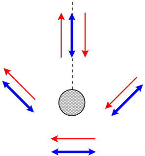
Figure 1: This figure shows the Higgs field, the bidirectional arrow, configuration of an Alice flux in AED. It also shows that the generator of the $U(1)$ part of the unbroken gauge group is not single valued in the presence of such an Alice flux, i.e., a $U(1)$ charge gets charge conjugated when transported around an Alice loop.

Secondly, just as compact $U(1)$ gauge theory, AED contains magnetic monopoles, because $\Pi_{1}(U(1)\ltimes\mathbb{Z}_{2})=\mathbb{Z}$. As is well known the monopoles become instantons in 2-dimensional electrodynamics and lead to confinement of charge, see [3] and [4]. The potential between two static charges becomes linear and the string tension due to the instantons was determined by Polyakov in [4] and is given by:

$$T\propto g^{2}\exp{\left(-\frac{S_{inst}}{2g^{2}}\right)}\quad,$$ (1)

with $S_{inst}$ the action of the instanton in (2+1)-dimensions, or the mass of a monopole in (3+1)-dimensions, and $g$ the (dimension-full) coupling constant. In compact alice electrodynamics there are instantons as well, one therefore in principle expects the same confining potential between charges. However, as we will see, whether this confinement will be realized physically depends on the parameters in the model.

With respect to the monopoles/instantons in AED we have previously [5] made another observation, namely, that the core structure of a magnetic monopole may be unstable and deform into a ring of alice flux carrying a cheshire magnetic charge. This feature, however is not expected to bear on the confinement mechanism as such, because the core structure does not affect the long range behavior of the fields. We return to this point towards the end of the paper.

We see that indeed the topological structure of AED is richer than the topology of ordinary electrodynamics, as it supports topologically stable alice fluxes. In this paper we will show that these fluxes may have a dramatic influence on the infrared behavior of the potential between two static charges. In the infrared region the potential will not grow linearly as in ordinary compact electrodynamics, but the potential will saturate and become constant at a scale set by the mass of the alice flux. This follows from the fact that a static charge will be unstable under the creation of two alice fluxes and the possibility of (induced) cheshire charges carried by such a pair. We calculate the decay rate of a charge due to this instability, into a state where the charge is completely delocalized, i.e., virtually disappeared.

Before turning to a detailed treatment of this remarkable charge instability, it is useful to briefly discuss some generic features of the parameter space we are considering. To be as flexible as possible in separating the various dynamical aspects of the theory, we like to think of a lattice version of the theory (as discussed in [6]), because in that setting one can introduce different mass scales for the fluxes ($m_{f}$), for the monopoles ($m_{m}$), and possibly also for dynamical, charged degrees of freedom ($m_{q}$) by hand. Of course in continuum versions of the model (like the original $SO(3)$ broken to $U(1)\ltimes\mathbb{Z}_{2}$ model) one often finds that these physical scales may be linked and one is forced to restrict oneself to a smaller region of the parameter space then the one we explore in the remainder of this paper.

The paper is organized as follows. In section 2 we examine the classical configuration of a pair of alice fluxes in the presence of a charge. We determine the field line pattern of such a configuration and the energy gain due to the introduction of flux pair. In section 3 we analyze the resulting charge instability in a semi-classical approximation and determine the action of the bounce solution for some specific decay channels. In the concluding section we discuss the relevance of our results in the broader context where one also takes the instantons into account. In the appendix we introduce the notion of a so called magnetic cheshire current and point out its relation with electric cheshire charge.

2 Alice fluxes in the presence of a charge

In this section we examine the classical field configuration due to a pair of alice fluxes in the presence of a charge. We first analyze this situation qualitatively, which leads to the conclusion that the pair of alice fluxes will carry an induced (cheshire) dipole charge. To see what that looks like we determine the configuration of electric field lines generated by a conducting needle between two oppositely charged point charges. The conducting needle represents a pair of alice fluxes (one at either end) with their core structure ignored. Finally, we will determine the energy gain due to the introduction of the needle/flux pair.

2.1 The induced cheshire dipole

Let us now study the field configuration of a charge in the presence of an alice loop (i.e., a flux pair in two dimensions). Due to conservation and quantization of charge, field lines cannot cross an alice flux, a situation reminiscent to that of the Meissner effect in a super conductor. In fact, at first sight one would be tempted to interpret the whole collection of cheshire phenomena as a manifestation of some exotic form of electric and/or magnetic super conductivity in the core of an alice loop. However, this is not possible because the flux tube itself cannot carry electric/magnetic charge (see also [5]) or current. Let us now consider what happens if we create an alice loop in the neighborhood of a charge.

A first guess of how a radial field would be affected due to the creation of the alice loop might be the same as for the case of a super conducting loop, i.e., the field lines would be pushed away by the loop. However the analysis illustrated in figure 2 yields a very different picture. Some of the field lines close around the first flux while an equal number emanates from the sheet to close around the second flux and go off to infinity, see figure 2. Thus the total charge carried by the alice flux configuration stays zero, as it should, but the flux configuration acquires an induced electric (cheshire) dipole moment. For convenience we only examine cases where the flux pair lies on the line connecting the charges. The electric field lines have to be be perpendicular to the line segment between the two fluxes, because (i) the electric field lines need to change sign when going around a single flux and (ii) the reflection symmetry through the horizontal axis of the configuration.

(a) (b) (c) (d)

Figure 2:
A sequence of figures that leads to the correct field line configuration for two alice fluxes in the presence of a charge. Figure (a) shows a single charge in figure (b) a pair of fluxes is created in the vicinity of the charge but with the wrong field line pattern as follows from deforming $\mathbb{Z}_{2}$-gauge sheet, figure (c). The correct field line pattern is given in figure (d).

In certain symmetric configurations the $\mathbb{Z}_{2}$-sheet may be considered to act like a conducting plate from which follows that the charge is pulled towards the alice loop. Indeed, one should be careful with this analogy because the conducting plate boundary condition of the $\mathbb{Z}_{2}$-sheet only holds in the particular gauge that satisfies the obvious symmetry condition. In a general gauge the $\mathbb{Z}_{2}$-sheet has an arbitrary shape and cannot be interpreted as a conducting plate. On the other hand, the field line pattern closing partially around the first and the second flux is gauge invariant (i.e., the pattern is, but not the direction of the field lines). We conclude that the charge induces a dipolar cheshire charge on the alice loop (or in 2 dimensions, on the pair of fluxes). This is a natural generalization of the result obtained in [2], but, straightforward as the generalization may be, there is an important aspect to it. As we mentioned before, a system of two fluxes or an alice loop can be in the topologically trivial sector of the theory and thus may play a role in the dynamical response of the vacuum to an external charge.

The dipolar behavior of an alice flux pair in the presence of a charge can have important consequences. Just like a particle anti-particle pair, these pairs may contribute to the screening of a bare charge, but an even more drastic consequence is possible. The scenario runs as follows. One of the fluxes can absorb the point charge, after which the charge would be carried as a cheshire charge by the flux pair. This cheshire charge acts like a fictitious charge distribution along the line connecting the fluxes, generating a repulsive force between the two fluxes causing the fluxes to move away from each other. This would mean that the cheshire charge would increasingly spread and weaken, put more bluntly, it effectively just disappears. The fluxes would cause an extreme case of charge delocalization. So, in two dimensions it therefore appears that in these type of theories, charge may leak away, implying the absence of any (static) charge.

2.2 The field configuration

We now turn to the determination of the field configuration of a flux pair located between two oppositely charged point particles. We use the boundary conditions imposed by the fluxes but neglect the core structure of the fluxes. This boils down to calculating the electric field configuration of a conducting needle located between two oppositely charged point particles, where the needle lies on the line connecting the charges.

Two-dimensional electrostatics (i.e., potential theory) has the convenient property that it is conformally invariant. Exploiting this conformal invariance one can construct explicit solutions satisfying the boundary conditions imposed by the geometry we are interested in. We start with determining the solution of a charge in the presence of a conducting disc with the help of the method of images. Then we use a conformal transformation which maps this conducting disc into a conducting needle/flux pair, see figure 3. Since a conformal transformation is angle preserving, a conductor gets mapped to a conductor.

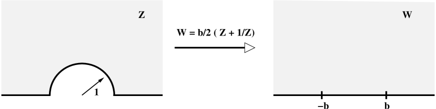
Figure 3: The conformal transformation, $w=\frac{b}{2}\left(z+\frac{1}{z}\right)$, which maps the conducting disc of radius one into a conducting needle of length $2b$.

To construct the configuration of two charges with a flux pair in between, we first determine the single charge case and then superpose two of these configurations. We determine the potential of a charge in the presence of a conducting disc with the help of the method of images. It is similar to the textbook example of the charge in the presence of a conducting ball in three dimensions, but for the case at hand the charge of the image charges does not depend on the distance of the charge to the conducting disc. Making use of the identity, $|\vec{n_{1}}+a\vec{n_{2}}|=|a\vec{n_{1}}+\vec{n_{2}}|$ with $|\vec{n_{1}}|=|\vec{n_{2}}|=1$, one easily finds the potential $\Phi(z)$, $z=x+iy$. The potential is given by:

$$\Phi(z)=\frac{Q}{2\pi}\left\{\log\left|z-z_{0}\right|-\log\left|z-\frac{R^{2}}{\left|z_{0}\right|^{2}}z_{0}\right|+\log|z|\right\}\quad,$$ (2)

with $R$ the radius of the conducting disc, whose center is located in the origin and $z_{0}$ denotes the location of the charge. The field lines correspond with the height lines of the function:

$$\Psi(z)=\frac{Q}{2\pi}\left\{\arg(z-z_{0})-\arg\left(z-\frac{R^{2}}{|z_{0}|^{2}}z_{0}\right)+\arg(z)\right\}\quad.$$ (3)

The results are plotted in figures 4a and 4b for the equipotential lines and the electric field lines respectively.

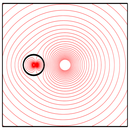
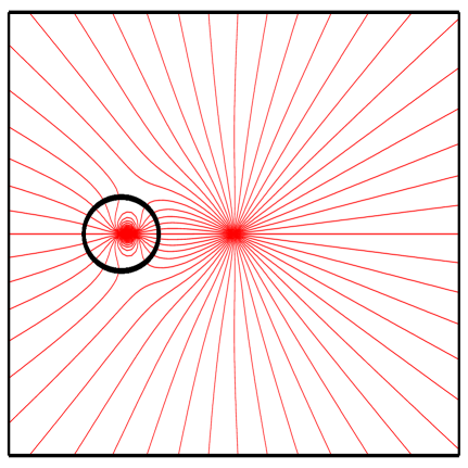
(a) (b)

Figure 4: These figures show some of the equipotential lines, figure (a), and field lines, figure (b), of a charge in the presence of a conducting disc. The thick dark circle is the boundary of the conducting disc. The configuration inside this circle represents the ’image’ charges.

We can use this solution to find the solution of a charge in the presence of a flux pair with the help of the conformal transformation given in figure 3. To be more general we first determine the configuration of two charges in the presence of a disc. This is straightforward since electrodynamics is linear in the sense that potentials just add. Thus for the situation of two (oppositely charged) charges we get the following potential:

$$\Phi(z)=\frac{Q}{2\pi}\left\{\log|z-z_{1}|-\log\left|z-\frac{R^{2}}{|z_{1}|^{2}}z_{1}\right|-\log|z-z_{2}|+\log\left|z-\frac{R^{2}}{|z_{2}|^{2}}z_{2}\right|\right\}\quad.$$ (4)

The field lines are now given by the height lines of the function:

$$\Psi(z)=\frac{Q}{2\pi}\left\{\arg(z-z_{1})-\arg\left(z-\frac{R^{2}}{|z_{1}|^{2}}z_{1}\right)-\arg(z-z_{2})+\arg\left(z-\frac{R^{2}}{|z_{2}|^{2}}z_{2}\right)\right\}\quad.$$ (5)

Let us now use the conformal transformation to map this solution to the solution of two charges in the presence of a flux pair located on the line connecting the charges. To be able to use the conformal map, of figure 3, $R$ needs to be unity. We can get the desired configuration if the two charges and the disc also lie on one line and the disc is between the two charges. We rotate the system such that $z_{1}$ and $z_{2}$ are real. After this we can use the conformal map to map this solution to the solution of the flux pair between two oppositely charged point charges. This is done by replacing $z$ by the corresponding function of $w$, which is given by: $z=x+\sqrt{x^{2}-1}$ where we have defined $x=\frac{w}{b}$ and will use corresponding definitions for $x_{1}$ and $x_{2}$. This gives the following potential:

$$\Phi(x) = \frac{Q}{2\pi}\left\{\log\left|x+\sqrt{x^{2}-1}-x_{1}-\sqrt{x_{1}^{2}-1}\right|\right.$$ (6)

$$-\log\left|x+\sqrt{x^{2}-1}-\frac{x_{1}+\sqrt{x_{1}^{2}-1}}{\left|x_{1}+\sqrt{x_{1}^{2}-1}\right|^{2}}\right|$$

$$-\log\left|x+\sqrt{x^{2}-1}-x_{2}-\sqrt{x_{2}^{2}-1}\right|$$

$$\left.+\log\left|x+\sqrt{x^{2}-1}-\frac{x_{2}+\sqrt{x_{2}^{2}-1}}{\left|x_{2}+\sqrt{x_{2}^{2}-1}\right|^{2}}\right|\right\}\quad,$$

and the field lines follow from:

$$\Psi(x) = \frac{Q}{2\pi}\left\{\arg\left(x+\sqrt{x^{2}-1}-x_{1}-\sqrt{x_{1}^{2}-1}\right)\right.$$ (7)

$$-\arg\left(x+\sqrt{x^{2}-1}-\frac{x_{1}+\sqrt{x_{1}^{2}-1}}{\left|x_{1}+\sqrt{x_{1}^{2}-1}\right|^{2}}\right)$$

$$-\arg\left(x+\sqrt{x^{2}-1}-x_{2}-\sqrt{x_{2}^{2}-1}\right)$$

$$\left.+\arg\left(x+\sqrt{x^{2}-1}-\frac{x_{2}+\sqrt{x_{2}^{2}-1}}{\left|x_{2}+\sqrt{x_{2}^{2}-1}\right|^{2}}\right)\right\}\quad.$$

The conformal transformation only correctly generates the solution in the upper half plane, $Re(x)>0$. The solution in the lower half plane follows by the obvious symmetry of the problem. In figure 5(a) and 5(b) we plotted the resulting equipotential and field lines for the configuration.

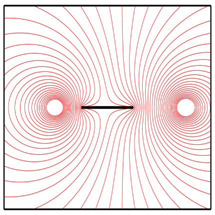
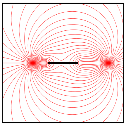
(a) (b)

Figure 5: These figures show some of the equipotential lines, figure (a), and field lines, figure (b), of two oppositely charged charges in the presence of the cheshire dipole carried by a pair of fluxes located at the endpoints of the black line segment.

2.3 The energy gain

In the previous subsection we determined the potential and the field configuration of a flux pair between two point charges. In this subsection we calculate the energy difference of this configuration with the (coulomb type) field configuration without the flux pair. To be able to determine the energy difference we have to regularize the expression, i.e., we introduce a UV cut off which will be removed later. With this cutoff the total energy difference is equal to the integrated energy density difference. Written in this form, the cutoff can be removed leaving the energy difference finite, and this is how we calculate the energy gain due to the presence of the flux pair. To simplify life the calculation is performed in $z$ space, not in $w$ space. So we use the conformal transformation, which is also just a convenient change of variables, to transform the solution back into $z$ space and as an intermediate step, determine the energy gain due to the presence of a conducting disc and the energy cost due to the presence of a magnetic super conducting disc. The energy gain due to the presence of a flux pair is determined from these two results. The relation between these energy differences is given by:

$$\int\{E_{dipole}-E_{fpair}\}dw=\int\{E_{mscdisc}-E_{disc}\}dz$$

$$=\int\{E_{dipole}-E_{disc}\}dz-\int\{E_{dipole}-E_{mscdisc}\}dz~{},$$ (8)

where $E_{mscdisc}$ is the energy density of two opposite charges with a disc in the middle, which we identify as a magnetic super conductor (msc) as the electric field lines are parallel to it. This configuration is the configuration that one obtains after applying the inverse conformal transformation, thus from $w$-space to $z$-space, to the dipole configuration in $w$-space. First we will determine the energy gain due to the presence of a conducting disc. This yields the expression:

$$\Delta E_{disc} = 2\int_{0}^{\pi}\int_{R}^{\infty}\left\{(\partial_{r}\Phi_{2}(r,\theta))^{2}+\left(\frac{1}{r}\partial_{\theta}\Phi_{2}(r,\theta)\right)^{2}\right.$$ (9)

$$\left.-~{}(\partial_{r}\Phi_{1}(r,\theta))^{2}-\left(\frac{1}{r}\partial_{\theta}\Phi_{1}(r,\theta)\right)^{2}\right\}r~{}drd\theta$$

$$+~{}2\int_{0}^{\pi}\int_{0}^{R}\left\{(\partial_{r}\Phi_{2}(r,\theta))^{2}+\left(\frac{1}{r}\partial_{\theta}\Phi_{2}(r,\theta)\right)^{2}\right\}r~{}drd\theta\quad,$$

with $\Phi_{1}(r,\theta)$ given by formula 4 and $\Phi_{2}(r,\theta)$ is given by formula 4 with $R=0$. This gives:

$$\Delta E_{disc}=-\frac{Q^{2}}{2\pi}\log\left(\frac{(z_{1}^{2}-R^{2})(z_{2}^{2}-R^{2})}{(z_{1}z_{2}+R^{2})^{2}}\right)\quad.$$ (10)

The energy gain due to the presence of a magnetically super conducting (msc) disc is determined by:

$$\Delta E_{mscdisc} = 2\int_{0}^{\pi}\int_{R}^{\infty}\left\{(\partial_{r}\Phi_{2}(r,\theta))^{2}+\left(\frac{1}{r}\partial_{\theta}\Phi_{2}(r,\theta)\right)^{2}\right.$$ (11)

$$\left.-~{}(\partial_{r}\Phi_{3}(r,\theta))^{2}-\left(\frac{1}{r}\partial_{\theta}\Phi_{3}(r,\theta)\right)^{2}\right\}r~{}drd\theta$$

$$+~{}2\int_{0}^{\pi}\int_{0}^{R}\left\{(\partial_{r}\Phi_{2}(r,\theta))^{2}+\left(\frac{1}{r}\partial_{\theta}\Phi_{2}(r,\theta)\right)^{2}\right\}r~{}drd\theta\quad,$$

with $\Phi_{1}(r,\theta)$ given by formula 4 and $\Phi_{3}(r,\theta)$ by:

$$\Phi_{3}(z)=\frac{Q}{2\pi}\left\{\log\left|\left(z+\frac{1}{z}\right)-\left(z_{1}+\frac{1}{z_{1}}\right)\right|-\log\left|\left(z+\frac{1}{z}\right)-\left(z_{2}+\frac{1}{z_{2}}\right)\right|\right\}\quad.$$ (12)

One obtains:

$$\Delta E_{mscdisc}=\frac{Q^{2}}{2\pi}\log\left(\frac{(z_{1}^{2}-R^{2})(z_{2}^{2}-R^{2})}{(z_{1}z_{2}+R^{2})^{2}}\right)\quad.$$ (13)

For the case of $R=1$ we have $E_{fpair}=\Delta E_{disc}-\Delta E_{mscdisc}$. Thus we get:

$$E_{fpair}=-\frac{Q^{2}}{\pi}\log\left(\frac{(z_{1}^{2}-1)(z_{2}^{2}-1)}{(z_{1}z_{2}+1)^{2}}\right)\quad.$$ (14)

This result is still in $z$ language, i.e., $z_{1}$ and $z_{2}$ need to be written in terms of $w_{1}$ and $w_{2}$. This is done with the help of the conformal transformation, $z=x+\sqrt{x^{2}-1}$, and leads to the following expression for the energy gain:

$$E_{fpair}=\frac{Q^{2}}{\pi}\log\left(\frac{1}{2}\left(1+\frac{1+x_{1}x_{2}}{\sqrt{x_{1}^{2}-1}\sqrt{x_{2}^{2}-1}}\right)\right)\quad.$$ (15)

We see that the energy gain due to creating a flux pair between two charges is basically unbounded. Moving the flux pair closer to one or both of the charges increases the energy gain. One expects that due the renormalization of the charge this would not go on for ever, effectively one expects an effective UV cutoff.

Let us now investigate the single charge configuration, i.e., we send one of the charges to infinity. In this case the energy gain is given by:

$$E_{fpair}=-\frac{Q^{2}}{\pi}\log\left(\frac{4\sqrt{d}}{\left(1+\sqrt{d}\right)^{2}}\right)\quad,$$ (16)

where $d$ is the ratio of the distance of the two fluxes to the charge.
We find that the energy gain due to the presence of the flux pair only depends on the ratio of the distance of the two edges to the charge. Thus no matter what the size is of the UV cutoff, the flux radius or in fact any other length scale, the energy gain can always be as large as one wants in a region where all length scales are insignificant with respect to the distances of the fluxes to the charge and between the fluxes. This shows that in two dimensions a single charge is always unstable (or meta-stable) with respect to a decay into a flux pair with a cheshire charge no matter what the length scales are. However, the length scales of course drastically change the decay time of a charge.

3 The charge instability

In this section we analyze a novel type of instability in the electric field of a charge. We pointed out before, that a pair of alice fluxes in the presence of a charge acquires an induced dipole, subsequently we determined the energy gain due to the creation of such pair. This raises the question to what extend the electric field configuration of a pair of static localized charges remains stable with respect to flux pair creation. We study this question in a lattice version of AED (LAED). The reason is, as mentioned in the introduction, that LAED allows us to introduce independent parameters, a mass $m_{f}$ for the alice flux and a mass/action $m_{m}$ for the monopole/instanton. First we analyze the charge instability, then we will determine what the decay time is and compare it with the instability under the creation of a pair of charged point particles (with mass $m_{q}$), assuming that these are present in the theory. To what extend these results can be carried over to a continuum version of the theory will be discussed in the concluding section.

Before turning to the the detailed calculations, let us make some general observations concerning the role of the various mass scales in the model. If both $m_{m}$ and $m_{f}$ are very large, a charge in two dimensions generates the well known logarithmic potential in the classical (small $g^{2}$) limit.:

$$V(r)=\frac{Q^{2}}{\pi}\log\left(\frac{r}{r_{0}}\right)\quad,$$ (17)

with $r_{0}$ some UV cutoff. Needless to say that the presence of dynamical charges in the model would (a) give rise to the standard (short distance) renormalization of the charge and (b) provide a cutoff to the potential at an energy of the order of mass of the charged particles $m_{q}$. If the monopole mass $m_{m}$ comes down and $m_{f}$ remains very large we get that the monopoles cause confinement, i.e., a linearly rising potential and the role of dynamical charges would be very much the same as for the logarithmic case. For the moment however, we will assume that no charged dynamical particles are present in the model (i.e., we assume them to be very massive). If now the flux mass comes down as well, then of course we get the possibility to dynamically create flux pairs out of the vacuum and these will cause the decay of the electric fields generated by the external charges. One expects a situation to arise where the potential (irrespective of its character) basically saturates and turns into a constant at a distance $(r/r_{0})$ where fieldenergy becomes comparable to the value $2m_{f}$.

3.1 The life time of charge

Let us now compute the decay time of a system of two charges by performing an instanton calculation in the spirit of the “false vacuum” as described by Coleman and Callan [7], [8]. To lowest order in $\hbar$ one only needs to determine the bounce solution with lowest action. The bounce is a classical solution of the Euclidean system, i.e., with the original potential inverted. In the mechanical analogue a classical particle moves from the meta stable point to the corresponding point at the other side of the barrier and back again. The instability, i.e., the tunneling through the barrier corresponds to half the Euclidean bounce solution, after which a real Minkovski time evolution takes over. At this point the system is not yet in its final state, but one expects that the new lowest energy state will be reached by emitting/dissipating energy through conventional (in this model presumably primarily electromagnetic) radiation processes. In the mechanical system with the inverted potential one should then find the particle trajectory with minimal action $S_{b}$. In the semi-classical domain the decay time is given by:

$$\tau\propto e^{\frac{S_{b}}{\hbar}}$$ (18)

In our system we find two extremal paths. We expect one of these two to have the lowest action, independent of the distance $2w$ between the two external charges. In the following we analyze the situation for two cases, firstly we will determine the action for the instability due to the creation of a flux pair, then we do the same for the creation of a pair of point charges and finally we compare both mechanisms.

We first consider the case where the pair of fluxes or of charges are created in the most symmetric way. This means that they start out exactly between the external charges. The other decay channel we investigate corresponds to the most asymmetric configuration, where the fluxes or charges are created in the vicinity of one of the external charges and only one flux or charge will move. The other flux or charge remains with the charge at a fixed minimal distance $R_{0}$, which represents the UV cutoff of the bare charge. We will also determine the action of the bounce - the pair creation rate - in a constant electric field.

So the calculations we are about to make for the various cases are very similar, so let us, before providing the specific details for each case, give the general structure of the results.

In the previous sections we have calculated the energy gain $E$ in the electric field due to the pair creation. From that we can determine the potential $V_{pair}$ for the creation of a pair as a function of their separation $2b$ and of course also dependent on the other fixed parameters that characterize the configuration, such as the external charges $Q$, their separation $w$, the masses $m_{f}$ $($or $m_{q})$ and sometimes a core size $R_{0}$.

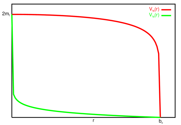
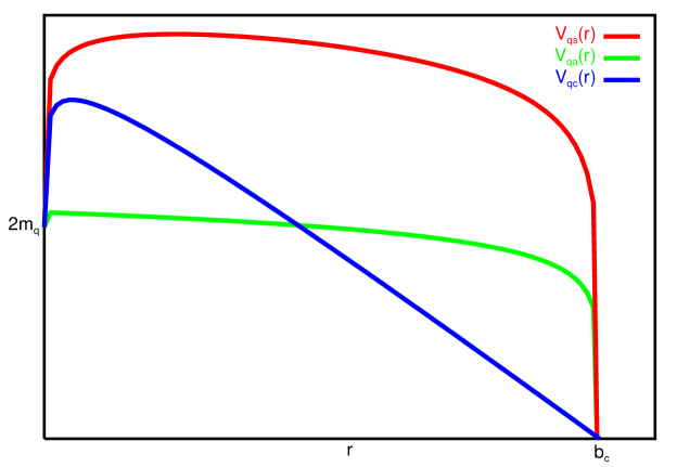
(a) (b)

Figure 6: In figure (a) we plotted two typical potentials for the bounce of two alice fluxes in the symmetric and asymmetric channel respectively. In figure (b) we plotted two typical potentials for the bounce of two dynamical charges in the symmetric and asymmetric channel respectively and the potential for the bounce of two dynamical charges in a constant field.

We have indicated the generic shape of the potentials in figures 6(a) and 6(b) for the pair creation of fluxes and dynamical charges respectively. For the fluxes we have assumed there to be no flux-flux interactions so that only the mass $2m_{f}$ comes in. For the charged pair, however one expects the potential to grow with separation which means that the maximum of the potential is shifted towards larger separation. As is well known in one dimensional physics, the action of the extremal path generically is given by:

$$S^{pair}=2\int_{b=0}^{b=b_{c}}\sqrt{4mV_{pair}}~{}db$$ (19)

We can bring this expression in a more or less canonical form. One first introduces a dimensionless separation variable $y$ obtained by conveniently scaling $b$ with some relevant length scale, for example the critical separation $b_{c}$ labeling the turning point, this brings out a factor of the relevant length scale out in front. Next one scales the potential by its maximal value: $V=V_{max}\hat{V}$. $V_{max}$ may conveniently be written as $V_{max}=2m\gamma^{2}$ where $\gamma$ is a dimensionless quantity satisfying $\gamma\geq 1$ and the equal sign applies to the flux pair creation (see figures). Putting the scaling factors in front of the integral the expression for the action takes the general form,

$$S^{pair}=const.\times b_{c}~{}m~{}\gamma~{}F(w,m,Q,R_{0})$$ (20)

where the dimensionless function $F$ may depend on all the parameters, but, because of the rescalings, takes on only values between zero and one.

$$F=\int_{y=0}^{y=1}\sqrt{\hat{V}_{pair}}~{}dy$$ (21)

We see that the action is typically of the order (mass of pair)x(critical separation), as one would expect naively. Yet, we will study the various cases separately in more detail, because it turns out that there are interesting differences in the functional dependence of $S^{pair}$ on for example the distance $w$ of the external charges, which are important physically.

3.1.1 Charge decay due to creation of an alice flux pair

We compute the action for a bounce corresponding with the creation of a flux pair in the presence of two external charges. First we consider the symmetric channel, then the asymmetric channel and finally the case of a constant electric field.

The symmetric channel:

In the symmetric channel we may use formula 15 with $x_{1}=x_{2}=x$, which gives the energy gain:

$$E_{fpair}=-\frac{Q^{2}}{\pi}\log\left(1-\frac{1}{x^{2}}\right)\quad.$$ (22)

During the bounce the external charges remain fixed while the distance between the fluxes increases. The suitably scaled variable for this situation is $y\equiv\frac{1}{x}=\frac{b}{w}$. So far we only determined the energy gain due to the boundary conditions created by the alice fluxes, but the potential in which the fluxes move is not only given by the energy gain, we also should include the energy cost which equals the mass of the flux pair, $2m_{f}$. The potential for the pair is therefore given by:

$$V_{fpair}=2m_{f}\left(\Theta\left(|y|\right)+\frac{1}{\mu}\log\left(1-y^{2}\right)\right)\quad,$$ (23)

where $\Theta(0)=0$ and equals one otherwise. The constant $\mu$ is defined as $\mu=\frac{2\pi m_{f}}{Q^{2}}$. We should note that keeping $y_{1}=y_{2}=y$ for all times is in fact a solution to the equations of motion for the system with the inverted potential. The action of this solution is simply given by:

$$S^{f}_{sym}=4\sqrt{2}~{}b_{c}~{}m_{f}F^{f}_{sym}(\mu)$$ (24)

where the turning points are given by the zeros of the potential, i.e.

$$b_{c}=w~{}\sqrt{1-e^{-\mu}}$$ (25)

and where $F^{f}_{sym}(\mu)$ is given by:

$$F^{f}_{sym}(\mu)=\int_{0}^{1}\sqrt{1+\frac{1}{\mu}\log\left(1-y^{\prime 2}\left(1-e^{-\mu}\right)\right)}~{}dy^{\prime}\quad.$$ (26)

Note that the function $F^{f}_{sym}$ depends in this case only on one particular combination of parameters, $\mu$. The integrand varies from one at $y=0$, to zero at $y=1$. Although the integral cannot be done analytically, a little analysis shows that the function always lies between the functions $f(y)=\sqrt{1-y^{2}}$ and $f(y)=1$. The integrals of these functions are easily determined to be $\frac{\pi}{4}\approx 0.8$ and one. So we have that $\frac{\pi}{4}\approx 0.8\leq F^{f}_{sym}(\mu)\leq 1$ which is indeed correct as one can see from the numerical evaluation of $F^{f}_{sym}(\mu)$ plotted in figure 7.

As mentioned before we need to introduce a UV cutoff for the bare charges, allowing the fluxes to approach a charge only up to a minimal distance $R_{0}$. One way to put this is that for the symmetrical process to be able to take place, or for that matter any decay mode using fluxes, $w$ needs to exceed a minimal value depending on $R_{0}$ and $\mu$. This constraint on $w$ is easily determined with the help of formula 23 by putting $b=w-R_{0}$ in other words $y=1-r_{0}$ with $r_{0}=R_{0}/w$. Determining the zero of the potential than gives the minimal value of $w$, yielding:

$$\frac{1}{r_{0}}=\frac{w}{R_{0}}\geq 2e^{\mu/2}\left(e^{\mu/2}+\sqrt{e^{\mu}-1}\right)\quad.$$ (27)

The asymmetric channel:

The asymmetric channel is the channel where one of the fluxes stays close to one of the charges and the other flux moves away. An interesting fact about this decay channel is, that in the limit of widely separated charges, $w\to\infty$, this channel will still give a finite decay time, whereas the symmetric channel would not. The energy gain due to the presence of a flux pair in this system again follows from formula 15. We fix one of the fluxes at the minimal cut-off distance $R_{0}$ from one of the charges. The other flux is pushed away from this charge. In this case it is natural to scale the variables by the core size $R_{0}$ as this is the only length scale in the limit of $w\to\infty$, so we define $\tilde{w}=\frac{w}{R_{0}}$ and $\tilde{y}=\frac{b}{R_{0}}$. The energy gain of this configuration is given by:

$$E_{fpair}=\frac{2m_{f}}{\mu}\log\left(\frac{1}{2}\left(1+\frac{2\tilde{w}(1+\tilde{y})-1-2\tilde{y}}{\sqrt{(2\tilde{w}-1)(2\tilde{w}-2\tilde{y}-1)(2\tilde{y}+1)}}\right)\right)\quad.$$ (28)

The potential is obtained by adding the mass term for the creation of the two alice fluxes out of the vacuum. The action of the bounce is determined in the same manner as we did in formula 19, not only do we have a different potential, we also need to change a factor $4$ into $2$, because only one flux is moving in this decay channel. For the action we obtain the following expression:

$$S^{f}_{asym}=4~{}m_{f}~{}b_{c}~{}F^{f}_{asym}(\mu,\tilde{w})\quad,$$ (29)

where the critical separation $b_{c}$ is given by:

$$b_{c}=\frac{(2\tilde{w}-1)R_{0}}{2-2\tilde{w}+\frac{\tilde{w}\left(\cosh\left(\frac{\mu}{2}\right)+3\sinh\left(\frac{\mu}{2}\right)\right)}{\sqrt{e^{\mu}-1}}}\quad.$$ (30)

The function $F^{f}_{asym}(\mu,\tilde{w})$ is defined by:

$$F^{f}_{asym}(\mu,\tilde{w})=\int^{1}_{0}\sqrt{1-\frac{1}{\mu}\log\left(\frac{1}{2}\left(1+\frac{2\tilde{w}(1+\tilde{y}^{\prime}\tilde{y}_{c})-1-2\tilde{y}^{\prime}\tilde{y}_{c}}{\sqrt{(2\tilde{w}-1)(2\tilde{w}-2\tilde{y}^{\prime}\tilde{y}_{c}-1)(2\tilde{y}^{\prime}\tilde{y}_{c}+1)}}\right)\right)}d\tilde{y}^{\prime}\quad,$$ (31)

and depends also on the separation of the external charges $2\tilde{w}$. Although we do get a similar expression as in the symmetric case the integral in the asymmetric case is not that easily estimated, see figure 8 for a plot of $F^{f}_{asym}(\mu,\tilde{w})$ and figure 7 for the value this integral takes in the limit of $\tilde{w}\to\infty$.

The remarkable fact is that this action remains finite in the limit of $\tilde{w}\to\infty$. Thus the decay time of a single charge (i.e., of charge itself) is finite in two dimensional alice electrodynamics.

The constant field:

Next we investigate the decay width per volume of a constant electric field. The energy gain due to the presence of a flux pair in line with the electric field strength can be found from formula 22. We move the charges to infinity and increase $Q$ such that the ratio $Q/w$ is kept fixed and we define the electric field as ${\cal E}\equiv\frac{Q}{\pi w}$. The resulting energy gain due to the presence of a flux pair then equals:

$$E_{fpair}=\pi{\cal E}^{2}b^{2}\quad.$$ (32)

The action is easily determined to be:

$$S^{f}_{const}=\sqrt{2}\pi m_{f}b_{c}\quad,$$ (33)

where the critical separation is,

$$b_{c}=\sqrt{\frac{2m_{f}}{{\cal E}^{2}\pi}}\quad.$$ (34)

The result is of course independent of position as it determines the decay rate per unit volume of a constant electric field.

3.1.2 Charge decay time due to creation of point charges

Let us now investigate the field instability of a pair of external charges under the creation of two dynamical charges. Since point charges have a singularity in the field energy at the core we introduce again a cutoff $R_{0}$ to regulate some of the infinities in our calculations. First we will determine the energy gain due to the presence of two point charges. We denote the two initial charges as $C_{1}$ and $C_{2}$, the created charges as $D_{1}$ and $D_{2}$. We put the four charges on one line and obviously assume the charges to be alternating. Symbolically the energy gain can be written as:

$$E^{q}_{gain} = (C_{1}+C_{2})^{2}-(C_{1}+C_{2}+D_{1}+D_{2})^{2}$$ (35)

$$= -(D_{1}^{2}+D_{2}^{2}+2D_{1}D_{2})-2(C_{1}+C_{2})(D_{1}+D_{2})\quad.$$ (36)

The first part, $D_{1}^{2}+D_{2}^{2}$, has an infinite contribution at the cores of the charges and only these infinities will be removed, i.e., only in this term we cut away a disc with radius $R_{0}$ around the charges. Taking the origin halfway the two created charges and denoting the distances of the charges with respect to this origin $w_{1}$, $w_{2}$ and $b$, the energy difference $E^{q}_{gain}$ is given by:

$$E^{q}_{gain}=-\frac{Q^{2}}{\pi}\log{\left(\frac{2(x_{1}-1)(x_{2}-1)}{(x_{1}+1)(x_{2}+1)\tilde{r}_{0}}\right)}\quad,$$ (37)

with $x=\frac{w}{b}$ and $\tilde{r_{0}}=\frac{R_{0}}{b}$.
This is the change in energy due to the electrical field configuration. We still need to take the mass of the point charges into account. We assume that the point charges are created a distance $2R_{0}$ away from each other and the energy cost of this process we call $2m_{q}$. Thus the total energy gain is given by:

$$V_{qpair}=2m_{q}\left(1+\frac{1}{\nu}\log\left(\frac{(x_{1}-1)(x_{2}-1)(x_{1}+\tilde{r}_{0})(x_{2}+\tilde{r}_{0})}{(x_{1}-\tilde{r}_{0})(x_{2}-\tilde{r}_{0})(x_{1}+1)(x_{2}+1)\tilde{r}_{0}}\right)\right)\quad,$$ (38)

with $\nu=\frac{2\pi m_{q}}{Q^{2}}$.
Next we will use this energy gain to determine the action of the bounce in different channels of the decay process.

The symmetric channel:

In the symmetric channel the potential is given by:

$$V_{qpair}=2m_{q}\left(1+\frac{1}{\nu}\log\left(\frac{(y-1)^{2}(r_{0}+1)^{2}y}{(r_{0}-1)^{2}(y+1)^{2}r_{0}}\right)\right)\quad,$$ (39)

where we still use $y=\frac{1}{x}=\frac{b}{w}$ and $r_{0}=\frac{R_{0}}{w}$.
To determine the action of the bounce we need to determine:

$$S_{qpair}=2w\int^{y=y_{c}}_{y=r_{0}}\sqrt{4m_{q}V_{qpair}}~{}dy\quad.$$ (40)

This is a quite non-trivial integral. We will estimate this integral by slightly changing the boundary conditions. As the lower boundary condition we will not take $r_{0}$, but the point between $r_{0}$ and zero where $V_{qpair}=0$. Later we will estimate the part we add to the action by this change in the boundary conditions.
So first we will determine the integral:

$$S^{q,1}_{sym}=2w\int^{y=y_{c}}_{y=y_{-}}\sqrt{4m_{q}V_{qpair}}~{}dy\quad,$$ (41)

with $y_{c}$ and $y_{-}$ the two values of $y$ where $V_{qpair}$ is equal to zero and with $0<y_{-}<y_{c}<1$. This integral is still quite difficult. We can determine it up to a part that we evaluate numerically and understand quite well. The action can be written as:

$$S^{q,1}_{sym}=4\sqrt{2}m_{q}(b_{c}-b_{-})\gamma^{q}_{sym}F^{q}_{sym}(\lambda)\quad,$$ (42)

with $\gamma^{q}_{sym}=\sqrt{\frac{\lambda-\lambda_{min}}{\nu}}$, $\lambda=\nu+\log\left(\frac{(r_{0}+1)^{2}}{(r_{0}-1)^{2}r_{0}}\right)$, $\lambda_{min}=\log\left(\frac{1}{2}\left(11+5\sqrt{5}\right)\right)$ and $F^{q}_{sym}(\lambda)$ given by:

$$F^{q}_{sym}(\lambda)=\int^{1}_{0}\sqrt{\frac{1+\lambda^{-1}\log\left(\frac{(1-((y_{c}-y_{-})y^{\prime}+y_{-}))^{2}}{(1+((y_{c}-y_{-})y^{\prime}+y_{-}))^{2}}((y_{c}-y_{-})y^{\prime}+y_{-})\right)}{1-\frac{\lambda_{min}}{\lambda}}}~{}dy^{\prime}\quad,$$ (43)

with $y_{c}=b_{c}/w$ and $y_{-}=b_{-}/w$.
In figure 7 we have plotted a numerical evaluation of the function $(y_{c}-y_{-})F^{q}_{sym}(\lambda)$. We still need to estimate the part introduced by taking different boundary values. This may be estimated by the maximum of the integrand in the region between $y_{-}$ and $r_{0}$ times $r_{0}$. If $\left(-2+\sqrt{5}\right)>r_{0}$ $V_{qpair,max}=2m_{q}$ else $V_{qpair,max}=2m_{q}\sqrt{\frac{\lambda-\lambda_{min}}{\nu}}$. Thus we estimate this part of the action to be $S^{q,2}_{sym}$, which is typically much smaller than $S^{q,1}_{sym}$, as follows:

$$S^{q,2}_{sym} \leq 4\sqrt{2}m_{q}R_{0}\quad\mbox{if}\quad\left(-2+\sqrt{5}\right)>r_{0}$$ (44)

and else

$$S^{q,2}_{sym} \leq 4\sqrt{2}m_{q}R_{0}\sqrt{\frac{\lambda-\lambda_{min}}{\nu}}\quad.$$ (45)

The asymmetric channel:

In the asymmetric channel the potential is given by:

$$V_{qpair}=2m_{q}\left(1+\frac{1}{\nu}\log\left(\frac{2\tilde{y}(\tilde{w}-\tilde{y}-1)}{(\tilde{y}+1)(\tilde{w}-2)}\right)\right)\quad,$$ (46)

The action of the bounce is given by:

$$S^{q}_{asym}=4m_{q}b_{c}\gamma^{q}_{asym}F^{q}_{asym}(\nu,\tilde{w})\quad,$$ (47)

with $\gamma^{q}_{asym}=\sqrt{1+\frac{1}{\nu}\log\left(\frac{2\left(1-\sqrt{\tilde{w}}\right)^{2}}{\tilde{w}-2}\right)}$ and

$$b_{c} = R_{0}\left(\frac{1}{4}e^{-\nu}(2+2e^{\nu}(\tilde{w}-3)-\tilde{w}+\right.$$ (48)

$$\left.\sqrt{-8e^{\nu}(\tilde{w}-2)+(-2-2e^{\nu}(\tilde{w}-1)+\tilde{w})^{2}}\right)\quad,$$

and $F^{q}_{asym}(\nu,\tilde{w})$ is given by:

$$F^{q}_{asym}(\nu,\tilde{w})=\int_{0}^{1}\sqrt{\frac{1+\frac{1}{\nu}\log\left(\frac{2(\tilde{y}^{\prime}\tilde{y}_{c}+1)(\tilde{w}-\tilde{y}^{\prime}\tilde{y}_{c}-2)}{(\tilde{y}^{\prime}\tilde{y}_{c}+2)(\tilde{w}-2)}\right)}{1+\frac{1}{\nu}\log\left(\frac{2\left(1-\sqrt{\tilde{w}}\right)^{2}}{\tilde{w}-2}\right)}}~{}d\tilde{y}^{\prime}.$$ (49)

In the limit $\tilde{w}\to\infty$ we can determine the integral exactly, yielding:

$$F^{q}_{asym}(\nu,\infty)=\frac{4e^{\nu}-\frac{\sqrt{\pi}~{}\mbox{Erfi}[\sqrt{\nu+\log(2)}]}{\sqrt{\nu+\log(2)}}}{4e^{\nu}-2}\quad.$$ (50)

Plots of $F^{q}_{asym}(\nu,\tilde{w})$ and $F^{q}_{asym}(\nu,\infty)$ are given in figures 8 and 7.

We recall that in the asymmetric channel for the creation of alice fluxes the result remains finite in the limit of widely separated external charges, obviously this is not the case for the action of the bounce corresponding to the creation of a pair of point charges.

The constant field:

Finally we will consider the case of a constant electric field and examine the action of the bounce if two point charges are created. To determine the energy gain in the field configuration we can use formula (38). However we cannot take the charge of the initial charges equal to the charge of the created point charges. To get the configuration in a finite electric field we take the distance between the initial charges to infinity while keeping the charge over the distance ratio fixed. Again we take the electric field ${\cal E}=\frac{Q_{initial}}{w\pi}$. The potential for the creation of two point charges in a constant electric field is given by:

$$V_{qpair}=2m_{q}\left(1+\frac{1}{\nu}\left(\log(\tilde{y})-u(\tilde{y}-1)\right)\right)\quad,$$ (51)

with $u=\frac{4\pi{\cal E}R_{0}}{Q^{2}}$.
The action of the bounce is given by:

$$S^{q}_{const}=2R_{0}\int^{\tilde{y}=\tilde{y}_{c}}_{\tilde{y}=1}\sqrt{4m_{q}V_{qpair}}~{}d\tilde{y}\quad.$$ (52)

Just as in the symmetric channel we take slightly different boundary conditions and estimate the difference later on. We will use the two values of $\tilde{y}$ where $V_{qpair}=0$ and we get:

$$S^{q,1}_{const}=2R_{0}\int^{\tilde{y}=\tilde{y}_{c}}_{\tilde{y}=\tilde{y}_{-}}\sqrt{4m_{q}V_{qpair}}~{}d\tilde{y}\quad.$$ (53)

This leads us to:

$$S^{q,1}_{const}=4m_{q}(b_{c}-b_{-})\gamma^{q}_{const}F^{q}_{const}(\kappa)\quad,$$ (54)

with $\gamma^{q}_{const}=\sqrt{\frac{\kappa-1}{\nu}}$, $\kappa=\nu-\log(u)+u$, $b_{c}\frac{u}{R_{0}}=\left(\tilde{y}_{c}^{\prime}=\right)\kappa+\log(\kappa+\log(\kappa+\log(\kappa+\cdots)))$ and $b_{-}\frac{u}{R_{0}}=\left(\tilde{y}_{-}^{\prime}=\right)\exp(-\kappa+\exp(-\kappa+\exp(-\kappa+\cdots)))$, where $\tilde{y}_{c}^{\prime}$ and $\tilde{y}_{-}^{\prime}$ are the two real solutions of $\kappa+\log(\tilde{y}^{\prime})-\tilde{y}^{\prime}=0$. $F^{q}_{const}(\kappa)$ is a function which varies only from $\frac{\pi}{4}$ at $\kappa\to 1$ to $\frac{2}{3}$ at $\kappa\to\infty$ and is given by:

$$F^{q}_{const}(\kappa)=\int^{1}_{0}\sqrt{\frac{\kappa+\log((\tilde{y}_{c}^{\prime}-\tilde{y}_{-}^{\prime})\tilde{y}^{\prime}+\tilde{y}_{-}^{\prime})-((\tilde{y}_{c}^{\prime}-\tilde{y}_{-}^{\prime})\tilde{y}^{\prime}+\tilde{y}_{-}^{\prime})}{\kappa-1}}~{}d\tilde{y}^{\prime}$$ (55)

see figure 7 for a plot of $F^{q}_{const}(\kappa)$.
We still need to estimate the part we introduced by taking different boundary values. We approximate that part by the maximum of the integrand in the region between $\tilde{y}_{-}$ and $1$ times $R_{0}$. If $u<1$ then $V_{qpair,max}=2m_{q}$ and otherwise $V_{qpair,max}=2m_{q}\left(\frac{\kappa-1}{\nu}\right)$. Thus the upperbound for this part of the action, $S^{q,2}_{const}$, is typically much smaller than $S^{q,1}_{const}$, to be explicit:

$$S^{q,2}_{const} \leq 4\sqrt{2}m_{q}R_{0}\quad\mbox{if}\quad u<1$$

else

$$S^{q,2}_{const} \leq 4\sqrt{2}m_{q}R_{0}\sqrt{\frac{\kappa-1}{\nu}}\quad.$$ (57)

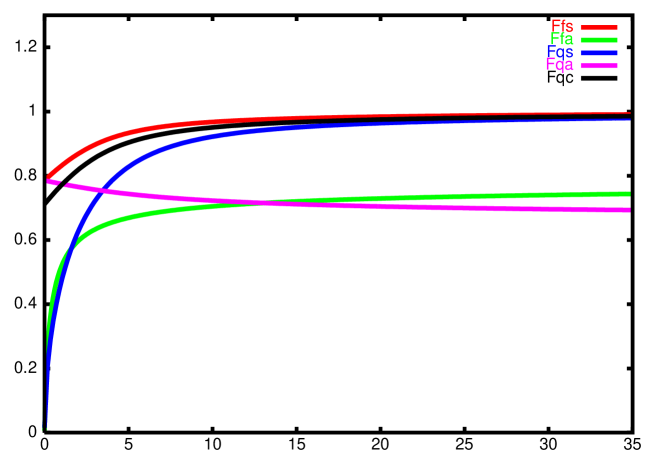
Figure 7:
This figure shows the five functions $Ffs=F^{f}_{sym}(\mu)$, $Ffa=F^{f}_{asym}(1/\mu)$, $Fqs=(y_{c}-y_{-})F^{q}_{sym}(\lambda-\lambda_{min})$, $Fqa=F^{q}_{asym}(\nu)$ and $Fqc=F^{q}_{const}(\kappa-1)$ numerically, with $\lambda_{min}=\log\left(\frac{1}{2}\left(11+5\sqrt{5}\right)\right)$, $F^{q}_{asym}(\nu)=F^{q}_{asym}(\nu,\infty)$ and $F^{f}_{asym}(1/\mu)=F^{f}_{asym}(1/\mu,\infty)$

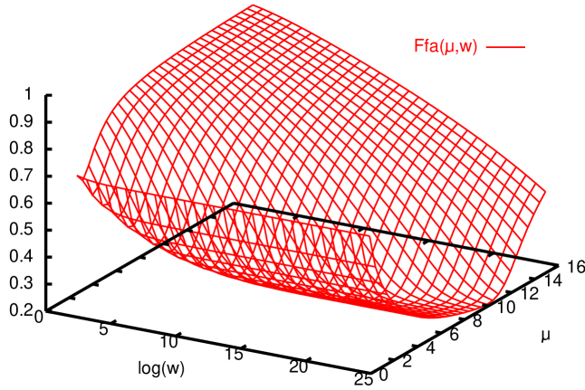
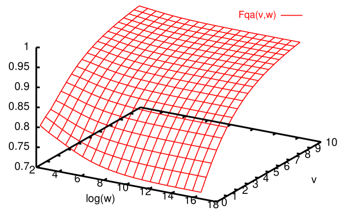
(a) (b)

Figure 8:
Figure (a) shows a plot of $F^{f}_{asym}(\mu,\tilde{w})$. The figure shows that the limit of the integral at $\tilde{w}\to\infty$ is reached only very slowly. The minimum value of the integral only moves slowly to large $\mu$ as $\tilde{w}$ grows exponentially. Figure (b) shows a plot of $F^{q}_{asym}(\nu,\tilde{w})$. The figure shows that the limit of of the integral at $\tilde{w}\to\infty$ is reached very fast. In the limit of $\tilde{w}\to\infty$ we know the integral exactly.

3.1.3 Comparing the decay channels

We just determined the actions of bounce solutions corresponding to some decay channels of two static point charges. As expected the action depends strongly on the parameters of the model. LAED allows for the different parameters to be independent of each other, so there are many possibilities for the preferred decay channel. Although the LAED model we described before does not require dynamical charges we did determine the action of some decay channels for the creation of pairs of such charges. Both dynamical charges and alice fluxes can render the static point charge configuration unstable. However, the decay time will typically depend exponentially on the distance between the two static charges except for one possible mode: the asymmetric decay channel of the two static charges under the creation of two alice fluxes. The action of this channel saturates. This means that the even the decay width of a single point charge is finite in AED, this obviously in contrast with ordinary ED. This instability is the process mentioned at the end of section 2.1, which may be considered as the two dimensional dual analog of the monopole core instability described in [5]. This implies basically the nonexistence of static charges in the theory, and that is the main observation we make in this paper.

We already mentioned that a pair of alice fluxes can be represented by a conducting needle in our configurations. On a conductor charges are free to move and one can for example have an induced dipole moment. In this picture the creation of two point charges is just a highly singular charge distribution on this line segment and it is obvious that the action of the bounce for alice fluxes can always be made lower because the charge distribution can still be varied. A simple and extreme example is the asymmetric channel in the limit of $\tilde{w}\to\infty$. Here the action of the bounce for the point charges is infinite while the action of the bounce for the alice fluxes remains finite.

4 Conclusions and outlook

In this paper we have extensively analyzed the behavior of alice fluxes in the presence of electric charges in (2+1)-dimensions. We showed that a pair of alice fluxes in the presence of an electric charge develops an induced electric dipole moment. This dipole moment is of the cheshire type which means that it is carried by the flux pair, and that the would-be charges making up the dipole are strictly nonlocalizeable en thus remain elusive. Exploiting conformal invariance we determined the resulting field configurations exactly which in turn allowed us to calculate the energy gain due to the introduction of a pair of alice fluxes between two external charges. Subsequently we considered the stability using semi-classical methods, using a Euclidean bounce solution.

We used a lattice model of AED [6] to investigate the effects of alice fluxes on a configuration of static point charges, because it allowed us to investigate the effects of the different topological defects separately. In the case of heavy monopoles we found an instability in the charge configuration due to the creation of a pair of alice fluxes. Although this instability looks quite similar to the instability due to the creation of two dynamical point charges there is a crucial difference. In the limit of increasing separation between the static charges the decay time due to the creation of dynamical point charges diverges, while for the creation of two alice fluxes it saturates and remains finite. To reach this conclusion we did not have to calculate the fluctuation determinant in detail, assuming that it is finite. Consequently in (L)AED a single bare charge is unstable under the creation of two alice fluxes, which can be seen as the (2+1)-dimensional dual analog of the monopole core instability [5]. If the monopole mass moves down, i.e., the confinement scale comes into play, the instabilities due to a flux pair and a charge anti-charge pair become very similar. In figure 9 we have sketched the potential for a typical situation.

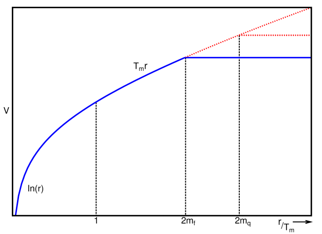
Figure 9: The effective potential for a pair of external charges. The figure represents the case where the mass of the alice flux pair is larger than the confinement scale, but smaller than the mass of dynamical charges. It is possible to lower $m_{f}$ below the confinement scale.

For the theory at hand we are presently determining these potentials through computer simulations in the lattice alice electrodynamics model [6] mentioned at the beginning of this paper and hope to report on these results in the near future.

Let us now give some comments on the continuum theory. We expect the situation to be not so much different. The topological defects arise as a consequence of spontaneous symmetry breaking, which means that the mass scales for the fluxes and monopoles might be much more constrained. We showed [5] that if the flux mass gets much less then the monopole mass, one may well get that the monopole decays in a flux ring carrying a cheshire magnetic charge. This suggests that the confinement scale and the instability scale (due to flux creation) cannot be too much different. As we explained, if the monopole and alice flux mass are comparable the potential still saturates due to the instability under the creation of two alice fluxes.

In this paper we showed that the possibility of cheshire charge in a theory has serious consequences for the stability of charge in the theory in two dimensions. It is usually a question of energetics what the stable configuration is, but for theories which allow for cheshire charges, a cheshire charge configuration is the natural second candidate to carry the charge. This suggests that any theory which breaks to a subgroup which contains a discrete and continuous component that do not mutually commute the gauge charges may well become unstable due to the cheshire phenomenon. Another interesting class of theories which typically contain cheshire charged configurations are the theories with non-abelian discrete gauge symmetries, which are best described with the help of a spontaneously broken Hopf symmetry [9, 10].

In the appendix of this paper we introduce an object called the (magnetic) cheshire current and we discuss its relation with (electric) cheshire charges. We will also discuss its relation with the closed electric field lines that occur if one interprets the occurrence of an instanton as an event in the (2+1)-dimensional (alice) electrodynamic setting. From this picture the confinement mechanism can be understood quite easily.

Acknowledgment: We thank Jan Smit for very useful discussions on the topics discussed in this paper. This work was partially supported by the ESF COSLAB program.

Appendix

Appendix A Cheshire current and confinement

In this appendix we will discuss the notion of a (magnetic) cheshire current in AED and the confinement of charges in (2+1)-dimensional (alice) electrodynamics [4]. We’ll introduce a configuration in AED named (magnetic) cheshire current and explain its relation with (electrical) cheshire charges and confinement in two dimensions. We’ll introduce a picture of two dimensional confinement from which qualitatively the confinement of the electrical flux into a flux tube comes apparent.

A.1 The cheshire current

Neither electric nor magnetic field lines are allowed to cross an alice flux, suggesting some exotic type of super conductivity through the core of the flux tube. In this part of the appendix we return to this analogy and find an interesting gauge complementarity between electric cheshire charges and a magnetic cheshire currents. Let us introduce the latter first.
Let us consider the following “gedanken” experiment. We create two charged particles from the vacuum and take one of the two particles around two spatially separated fluxes and then annihilate the two particles again. If the flux tubes are magnetic super-conductors this would have resulted in two magnetic current carrying fluxes, each with closed electric field lines around them. In the case of two alice fluxes a different picture emerges. Since the field lines cannot close around a single alice flux, one needs to take an even number of fluxes to be able to annihilate the particles again. This means that if one pulls the two fluxes apart one cannot be left with two fluxes which each carry a current. The field lines need to stay around both fluxes. A situation very different from the super conductors indeed. The system as a whole carries the current and just as in the case of a cheshire charge the current is non-localizeable; we should call this object a cheshire current.

The resulting field line configuration, depicted in figure 10, implies an attractive interaction between the two fluxes, on top of the normal flux interactions. It has the opposite effect of a cheshire charge, which leads to a repulsive force between the two fluxes.

Figure 10: Closed electric field lines of a (magnetic) cheshire current configuration.

Upon closer inspection we will see that there is a certain gauge complementarity, reconciling the two different pictures, describing non-localizeable alice effects. At first sight electric cheshire charge and a magnetic cheshire current appear to be very different entities. Let us now point out that there is actually a close relation between them. Imagine we repeat the gedanken experiment we just performed, but now we move in two more alice fluxes from infinity in such a way that all four of them are on one single line. As we know, on each flux one $\mathbb{Z}_{2}$ line should end. For convenience we put these half lines on top of the line on which we put the fluxes. For every flux we then still have the freedom to let the line go to the left or to the right. The result just yields two different, but gauge equivalent, configurations, as is illustrated by the top and bottom pictures in figure 11.

As we argued before, one can deform the $\mathbb{Z}_{2}$ lines in any way one wants by gauge transformations. From figure 11 it is clear that we can gauge transform the first configuration into the last one. This means that they both describe the same physics, although their interpretation appears to be quite different. In one case, see the bottom picture of figure 11, one would argue that two cheshire charges are the source of the field lines, but in the other situation, see the top picture of figure 11, one would argue that three cheshire currents are the source of the field lines. Apparently there are two different ways of looking at this configuration. As was explained before [1] one needs to cut away some region(s) of space-time if one wants to consider field strengths which are not single valued in the presence of an alice flux. However, there is of course not unique choice to do this. This freedom of choice corresponds exactly to the gauge complementarity of cheshire charge and cheshire current.

Figure 11: The ’duality’ transformation from three magnetic cheshire currents into two electric cheshire charges.

We do note that although they are related by a gauge transformations it does not mean that all configurations can be thought of as consisting only of cheshire charges or only of cheshire currents. A simple example is a pair of alice fluxes carrying a cheshire charge and a cheshire current. This object may in fact be a stable configuration in two dimensions, since the electric cheshire charge results in a repulsive force between the two fluxes whereas the magnetic cheshire current results in a attractive force between the two fluxes. These could be made to cancel leading to a stationary configuration.

A.2 Confinement in a two dimensional picture

In this subsection we will consider the confinement of (2+1)-dimensional electrodynamics. This problem was already solved in [4]. For any non-zero value of the gauge coupling constant (2+1)-dimensional electrodynamics is confining (in the quenched approximation). It is well known that the instanton density increases and polarizes around the minimal sheet bounded by a closed Wilson loop. In a three dimensional Euclidean space the instanton configuration is in fact just a magnetic monopole. After translating the instanton configuration to Minkovski space it is easy to understand that the polarization of the instanton density results in the confinement of the electrical flux into a flux tube.
By going to Minkovski space the interpretation of the fields change. The $z$-component of the magnetic field becomes the pseudo scalar magnetic field in the (2+1)-dimensional Minkovski space, while the $\theta$ and $\rho$ components of the magnetic field get translated into the $\rho$ and $\theta$ components of the electric field respectively. For the moment we will ignore the factors of $i$ as they will have no influence on the picture we use, although they do play an important role in the dynamics and the polarization of the instanton density.
Changing from Euclidean to Minkovski space allows us to interpreted the instanton density as a magnetic current density in Minkovski space. The nice thing of this two dimensional interpretation is that the confinement of the electrical flux into a flux tube easily follows from the superposition of the field lines of the pair of charges and the magnetic currents. In figure 12 we see that superimposing a magnetic current to the electric dipole configuration moves the field lines inwards. Indicating that a (polarized) magnetic current density would confine the electric flux into a flux tube.

(a) (b)

Figure 12: In figure (a) we plotted the field configuration of two opposite charges in the absence of instantons. In figure (b) we see that the introduction of magnetic currents, representing the instantons in Minkovski space, pushes the field lines inwards explaining the fact that the electric flux gets confined in a flux tube in the presence of a (polarized) instanton density.

In the previous section of this appendix we introduced an object in AED which can also be identified as a magnetic (cheshire) current. However the dynamics, due to the factors of $i$, is very different.

References

- [1] A. S. Schwarz. Field theories with no local conservation of the electric charge. Nucl. Phys., B 208:141, 1982.
- [2] Mark Alford, Katherine Benson, Sidney Coleman, John March-Russell, and Frank Wilczek. Zero modes of nonabelian vortices. Nucl. Phys., B 349:414–438, 1991.
- [3] A. A. Belavin, Alexander M. Polyakov, A. S. Shvarts, and Yu. S. Tyupkin. Pseudoparticle solutions of the Yang-Mills equations. Phys. Lett., B59:85–87, 1975.
- [4] A. M. Polyakov. Compact gauge fields and the infrared catastrophe. Phys. Lett., B59:82–84, 1975.
- [5] F. A. Bais and J. Striet. On a core instability of ’t Hooft Polyakov monopoles. Phys. Lett., B540:319–323, 2002.
- [6] J. Striet and F. A. Bais. Simulations of Alice electrodynamics on a lattice. Nucl. Phys., B647:215–234, 2002.
- [7] Sidney R. Coleman. The fate of the false vacuum. 1. Semiclassical theory. Phys. Rev., D15:2929–2936, 1977.
- [8] Jr. Callan, Curtis G. and Sidney R. Coleman. The fate of the false vacuum. 2. First quantum corrections. Phys. Rev., D16:1762–1768, 1977.
- [9] F. A. Bais, B. J. Schroers, and J. K. Slingerland. Hopf symmetry breaking and confinement in (2+1)-dimensional gauge theory. hep-th/0205114, 2002.
- [10] F. A. Bais, B. J. Schroers, and J. K. Slingerland. Broken quantum symmetry and confinement phases in planar physics. Phys. Rev. Lett., 89:181601, 2002.