Semiclassical wormholes

Abstract

Smooth-throat wormholes are treated on as possessing quantum fluctuation energy with scalar massive field as its source. Heat kernel coefficients of the Laplace operator are calculated in background of the arbitrary-profile throat wormhole with the help of the zeta-function approach. Two specific profile are considered. Some arguments are given that the wormholes may exist. It serves as a solution of semiclassical Einstein equations in the range of specific values of length and certain radius of wormhole’s throat and constant of non-minimal connection.

I Introduction

Great interest towards the space-time of wormholes dates back at least to 1916 Fla16 . Subsequent activity was initiated by both classical works of Einstein and Rosen in 1935 EinRos35 in the context of black hole space-time structure and the later series of works by Wheeler in 1955 Whe55 with his excellent idea to create everything from nothing. The more recent interest in the topic of wormholes has been rekindled by the works of Morris and Thorne MorTho88 and Morris, Thorne, and Yurtsever MorThoYur88 who made use of the concept of wormhole in scientific discussion of ”time machine”. These authors constructed and investigated a class of objects they referred to as ”traversable wormholes”. Their work led to a flurry of activity in wormhole physics VisserBook .

It is well-known that the central problem of the traversable wormholes connects with unavoidable violations of the null energy condition. It means that the matter which should be a source of this object has to possess some exotic properties. For this reason the traversable wormhole can not be represented as a self-consistent solution of Einstein equations with usual classical matter as a source because usual matter is sure to satisfy all energy conditions. One way out is to use quantum fields in frameworks of semi-classical quantum gravity. The point is that the vacuum average value of energy-momentum tensor of quantum fluctuations may violate energy conditions. A self-consistent wormholes in framework the semiclassical quantum gravity have been studied in Ref. Sus92 . In our recent paper KhuSus02 we have considered a possibility for self-consistent solution of semi-classical Einstein equations for specific kind of wormhole – short-throat flat-space wormhole. The model represents two identical copies of Minkowski space with spherical regions excised from each copy, and with boundaries of these regions to be identified. The space-time of this model is flat everywhere except a two-dimensional singular spherical surface. The vacuum average of energy of quantum fluctuations of massive scalar field with non-minimal connection serves as a source for this space-time. Due to the fact that this space-time is flat everywhere a complete set of wave modes of the massive scalar field can be constructed and ground state energy can be calculated. In the paper we present a calculation of full energy of quantum fluctuations rather then energy density and use the Einstein’s equations with quantum source only, without classical contribution. We found that the energy of fluctuations as a function of radius of throat $a$ may possess a minimum if the non-minimal connection constant $\xi>0.123$. Utilization of the Einstein equations at the minimum gives the stable configurations of the wormhole. For instance, in the case of conformal connection, $\xi=1/6$, we found relation between the radius $a$ of wormhole and mass $m$ of the scalar field: $am\approx 0.16$. The Einstein equations say that the wormhole has a radius of throat $a\approx 0.0141l_{Pl}$ and the mass of scalar field $m\approx 11.35m_{Pl}$. Therefore, this kind of wormhole, if it exists, may possess sub-Planckian radius of throat and it may be created by a massive scalar field with supper-Planckian mass. Obviously, the validity of the results obtained are restricted by the model taken – short-throat flat-space wormhole.

The goal of this paper is to consider the wormholes with more real geometry of throat and energy of quantum fluctuations of massive scalar field as a source of this background. The main problem in this case has rather mathematical character. Even for simple profile of throat it becomes impossible to obtain a full set of solutions of radial equation in order to find the energy density of quantum fluctuations in close form. Nevertheless, it is possible to make some predictions about the existence of the wormholes by considering the heat kernel coefficients KhuSus02 . In fact, the crucial point is the existence of the negative minimum of the zero point energy. The sufficient condition for the zero point energy to have negative minimum is that the heat kernel coefficients $B_{2}$ and $B_{3}$ be positive KhuSus02 . This gives a condition for parameters of model. More precisely, if a background is described by a parameter $\tau$ with dimension of length and the domain where the space-time is ”mainly” curved is defined by this parameter, then for small size of curved domain, $\tau\to 0$, the zero point energy shows the following behavior

$$E^{ren}\approx-\frac{B_{2}\ln(\tau m)^{2}}{32\pi^{2}},$$

and in opposite limit $\tau\to\infty$ we have

$$E^{ren}\approx-\frac{B_{3}}{32\pi^{2}m^{2}}.$$

If both these conditions are satisfied one can expect that the system will stay in minimum of energy which is characterized by specific values of parameters of wormhole and constant of non-minimal connection $\xi$. Next step is the utilization of the Einstein’s equations with energy-momentum tensor of quantum fluctuations as a source. Integration over volume the $t-t$ component of this equation gives an additional relation between parameters of wormhole and zero point energy by using which we obtain the size of wormhole and mass of scalar field in terms of the Planck length and Planck mass correspondingly. At the beginning we may expect KhuSus02 that the size of wormhole and mass of field will be in the Planck scale. For this reason we are interested only in finding of the domain of the wormhole’s parameters and constant non-minimal connection $\xi$ for different models of the wormhole’s profile.

The manifest expression for coefficient $B_{2}$ exists for arbitrary background, but this is not the case for coefficient $B_{3}$. For this reason we adopt here the zeta-regularization approach (see Sec. III), in frame of which it is possible to calculate the heat kernel coefficients and zero point energy itself. We pursue here another goal – to evolve the zeta-function approach for situations where it is impossible to find the full set of solutions of radial equation in closed form. We find a method to calculate the heat kernel coefficients in the background of wormhole with arbitrary profile of throat by using the WKB approach. Moreover, we obtain expressions for arbitrary heat kernel coefficients and we reproduce them in manifest form up to $B_{3}$ for arbitrary profile of wormhole’s throat.

The organization of the paper is as follows. In Sec. II we consider the geometry of wormhole with smooth throat. In Sec. III we discuss the method of zeta-function for calculation of zero-point energy. The WKB approach for scalar massive field is considered in Sec.IV. The heat kernel coefficients are obtained in Sec.V. We calculate them in manifest form for arbitrary profile of throat. The specific profiles of throat are investigated in Sec.VI and VII. In Sec.VIII we discuss the results obtained. Appendix A contains some technical formulas which are rather complicated to reproduce them in the text.

We use units $\hbar=c=G=1$. The signature of the space-time, the sign of the Riemann and Ricci tensors, are the same as in the book by Hawking and Ellis HawEllBook .

II A traversable wormhole with smooth throat

The metric of space-time of wormhole which is under consideration has the form below

$$ds^{2}=-dt^{2}+d\rho^{2}+r^{2}(\rho)(d\theta^{2}+\sin^{2}\theta d\varphi^{2}).$$ (1)

The radial variable $\rho$ changes from $-\infty$ to $+\infty$. In the paper we restrict ourself by wormholes with symmetric throat which means that $r(-\rho)=r(+\rho)$. The radius $a$ of throat is defined as follows $a=r(0)$. We suppose that far from the wormhole’s throat the space-time becomes Minkowskian, that is

$$\lim_{\rho\to\pm\infty}\frac{r^{2}(\rho)}{\rho^{2}}=1.$$

The non-zero components of the Ricci tensor and scalar curvature have the following form

$$\mathcal{R}^{\rho}_{\rho} = -\frac{2r^{\prime\prime}}{r},$$

$$\mathcal{R}^{\theta}_{\theta}=\mathcal{R}^{\varphi}_{\varphi} = -\frac{-1+r^{\prime 2}+rr^{\prime\prime}}{r^{2}},$$

$$\mathcal{R} = -\frac{2(-1+r^{\prime 2}+2rr^{\prime\prime})}{r^{2}}.$$

The energy-momentum tensor corresponding to this metric has diagonal form from which we observe that the source of this metric possesses the following energy density and pressure:

$$\varepsilon = -\frac{-1+r^{\prime 2}+2rr^{\prime\prime}}{8\pi r^{2}},\allowdisplaybreaks$$

$$p_{\rho} = \frac{-1+r^{\prime 2}}{8\pi r^{2}},\allowdisplaybreaks$$

$$p_{\theta} = p_{\varphi}=\frac{r^{\prime\prime}}{8\pi r}.$$

In the paper we obtain general formulas for space-time 1 with arbitrary symmetric function $r(\rho)$ obeying above Minkowskian condition. Two specific kinds of throat’s profile will be considered. In the first model the profile of throat has the following form:

$$r(\rho)=\sqrt{\rho^{2}+a^{2}},$$ (2)

where $a$ is radius of throat which characterizes wormhole’s size. The embedding into the three dimensional Euclidean space of the section of the space-time by surface $t=const,\theta=\pi/2$ is plotted in Fig.1(I) for two different values of radius of throat. In Euclidean space with cylindrical coordinates $(r,\varphi,z)$ this surface may be found in parametric form from relations: $r=r(\rho),z^{\prime}(\rho)=\sqrt{1-r^{\prime 2}}$. In this background there is the only nonzero component of the Ricci tensor which reads

$${\cal R}^{\rho}_{\rho}=-\frac{2a^{2}}{(\rho^{2}+a^{2})^{2}}.$$

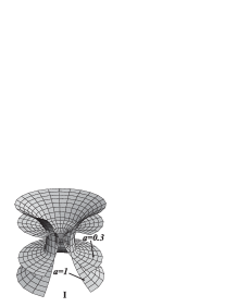
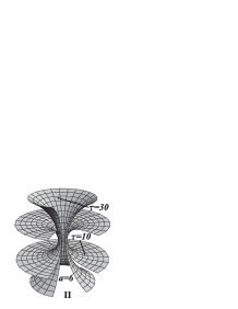
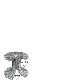
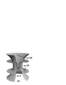
Figure 1: First figure (I) represents the section $t=const,\theta=\pi/2$ of wormhole’s space-time with profile function $r(\rho)=\sqrt{\rho^{2}+a^{2}}$ for two different values of radius of the throat. Three next figures illustrate the wormhole with profile of throat $r(\rho)=\rho\coth(\rho/\tau)-\tau+a$. Figure (II) and (III) illustrate that the $a$ and $\tau$ are radius and length of throat, accordingly. In last figure two wormholes with different $a$ but with the same ratio radius and length of throat are depicted. It is seen that the parameter $a$ characterizes the ”size” of wormhole and $\alpha$ describes the ”form” of wormhole.

The second model has been considered in Ref.Sus01 and it is characterized by the following profile of throat

$$r(\rho)=\rho\coth(\frac{\rho}{\tau})-\tau+a.$$ (3)

This model possesses a more reach structure. There are two parameters $\tau$ and $a$. The latter parameter is radius of throat. In this model we may introduce another parameter which may be called length of the throat. The point is that the function $r(\rho)$ turns into linear function of $\rho$ starting from distance $\rho>\tau/2$ and the space-time becomes approximately Minkowskian. Therefore, the length of throat $l=\tau$. Using new variables $y=\rho/a,\ \alpha=\tau/a$ one rewrites the function $r$ in the form below

$$r(y)=a(y\coth(\frac{y}{\alpha})-\alpha+1).$$

The parameter $\alpha$ is the ratio of the length and radius of throat. This parameter will play the main role in our analysis. It allows us to consider wormholes of different form, that is with different ratio of the radius and length of throat.

In Fig.1(II-IV) the sections $t=const,\theta=\pi/2$ of this wormhole space-time are shown for different values of $a$ and $\tau$. Namely in Fig.1(II) we represent two wormholes with the same radius of throat but with different length, and vice versa in Fig.1(II) we depict two wormholes with the same length of throat but with different radii of throat. In last picture Fig.1(IV) two wormholes with the same ratio of length and radius of throat, but with different values of throats’ radii are depicted. Therefore the size of wormhole with the same ratio of length and radius throat is managed by parameter $a$. The parameter $\alpha$ describes wormhole’s form.

III Zero point energy: zeta-function approach

We exploit the zeta function regularization approach DowCri76 ; ZetaBook developed in Ref. Bor95 and calculate the zero point energy of massive scalar field in this background with consequent using the Einstein equations. Let us repeat some main formulas from those papers. In framework of this approach the zero point energy

$$E(s)=\frac{1}{2}\mu^{2s}\sum_{j}\sum_{(n)}(\lambda_{(n),j}^{2}+m^{2})^{1/2-s}=\frac{1}{2}\mu^{2s}\zeta_{\mathcal{L}}(s-\frac{1}{2}),$$ (4)

of scalar massive field $\Phi$ is expressed in terms of the zeta-function

$$\zeta_{\mathcal{L}}(s-\frac{1}{2})=\sum_{j}\sum_{(n)}(\lambda_{(n),j}^{2}+m^{2})^{1/2-s}$$ (5)

of the Laplace operator $\mathcal{L}=-\triangle+m^{2}+\xi\mathcal{R}$. Here $\triangle=g^{kl}\nabla_{k}\nabla_{l}$ is the three dimensional operator. The eigenvalues $\lambda_{(n),j}+m^{2}$ of operator $\mathcal{L}$ are found from boundary condition which looks as follows

$$\Psi_{(n)}(\lambda,R)=0,$$ (6)

where $R$ denotes some boundary parameter. The solutions $\lambda=\lambda_{(n),j}$ of this equation depend on the numbers $(n)$, and additionally they have the index $j=1,2,\dots$, which numerates the solutions of the boundary equation. Therefore, the zeta-function is a sum of expressions which depend on zeros of function $\Psi_{(n)}$. Next, according to Ref.Bor95 we convert the series over $j$ in zeta function to integral and arrive to the formula

$$E(s)=-\frac{1}{2}\mu^{2s}\sum_{(n)}\frac{\cos\pi s}{\pi}\int_{m}^{\infty}dk(k^{2}-m^{2})^{1/2-s}\frac{\partial}{\partial k}\ln\Psi_{(n)}(ik,R),$$ (7)

where the function $\Psi_{(n)}$ in imaginary axes appears.

The expression 7 is divergent in the limit $s\to 0$ we are interested in. For renormalization we subtract from $E(s)$ all terms $E^{div}(s)$ which will survive in the limit $m\to\infty$:

$$E^{div}(s)=\lim_{m\to\infty}E(s)$$

and define the renormalized energy as follows:

$$E^{ren}=\lim_{s\to 0}(E(s)-E^{div}(s)).$$ (8)

Because the pole structure of zeta-function does not depend on the value of parameters, it is obvious that in the limit $m\to\infty$ the divergent part will have the structure of DeWitt-Schwinger expansion, which has the following form

$$E^{div}(s) = \frac{1}{2}\left(\frac{\mu}{m}\right)^{2s}\frac{1}{(4\pi)^{3/2}\Gamma(s-\frac{1}{2})}\allowdisplaybreaks$$

$$\times \left\{B_{0}m^{4}\Gamma(s-2)+B_{1/2}m^{3}\Gamma(s-\frac{3}{2})+B_{1}m^{2}\Gamma(s-1)+B_{3/2}m\Gamma(s-\frac{1}{2})+B_{2}\Gamma(s)\right\},$$

where $B_{\alpha}$ are the heat kernel coefficients. In order to extract the divergent part of the energy we use the following procedure Bor95 . We subtract from and add to integrand the uniform expansion of $\ln\Psi$ up to $m^{0}$. We denote this expansion as $(\ln\Psi_{(n)})^{as}$. Therefore, according to this, we represent the energy as the sum

$$E(s)=E_{fin}(s)+E_{as}(s)$$ (10)

of finite (in the limit $s\to 0$) part

$$E_{fin}(s) = -\frac{1}{2}\mu^{2s}\sum_{(n)}\frac{\cos\pi s}{\pi}\int_{m}^{\infty}dk(k^{2}-m^{2})^{1/2-s}\allowdisplaybreaks$$ (11)

$$\times \frac{\partial}{\partial k}\left(\ln\Psi_{(n)}(ik,R)-(\ln\Psi_{(n)}(ik,R))^{as}\right),$$

and the remains, which will be obtained from the uniform expansion part

$$E_{as}(s)=-\frac{1}{2}\mu^{2s}\sum_{(n)}\frac{\cos\pi s}{\pi}\int_{m}^{\infty}dk(k^{2}-m^{2})^{1/2-s}\frac{\partial}{\partial k}(\ln\Psi_{(n)}(ik,R))^{as}.$$

The last expression contains all terms which will survive in the limit $m\to\infty$.

Taking into account the obtained expressions in Eq. 8 we arrive at the formula

$$E^{ren}=E_{fin}+E_{as}^{fin},$$ (12a)

where

$$E_{fin} = E_{fin}(0)=-\frac{1}{2\pi}\sum_{(n)}\int_{m}^{\infty}dk\sqrt{k^{2}-m^{2}}\allowdisplaybreaks$$ (12b)

$$\times \frac{\partial}{\partial k}\left(\ln\Psi_{(n)}(ik,R)-(\ln\Psi_{(n)}(ik,R))^{as}\right),\allowdisplaybreaks$$

$$E_{as}^{fin} = \lim_{s\to 0}(E_{as}(s)-E^{div}(s)).$$ (12c)

The divergent part $E^{div}$ is given by Eq. III.

The finite part $E_{fin}$ is calculated numerically. The second part, in practice, is found in the following way. By using the uniform expansion $(\ln\Psi_{(n)})^{as}$ we calculate in manifest form the $E_{as}(s)$ and after that we take the limit $m\to\infty$ in the expression obtained (the pole structure does not change). All terms which will survive in this limit constitute the DeWitt-Schwinger expansion III which we have to subtract in Eq. 12c. This way of calculation is more preferable because we may obtain the heat kernel coefficients in manifest form. The calculations of heat kernel coefficients in framework of this approach shows that the approach is suitable for both smooth background and for manifolds with singular surfaces codimension one KhuSus02 and two KhuBor99 , the general formulas for which were obtained in Refs. GilKirVas01 and Fur94b .

From consideration above we may find the zero-point energy for large and small size of wormhole KhuSus02 . Let the parameter $a$ characterize the size of wormhole. In this case the $E^{ren}/m$ is a dimensionless function and it depends on the parameter $ma$ and some additional dimensionless parameters which characterize the form of wormhole. For example, in first model 2 there is the only parameter $a$ which is the radius of wormhole’s throat and it characterizes at the same time the size of wormhole as a whole. Therefore in this model the $E^{ren}/m$ depends on $ma$ and there are no additional parameters. In the second model 3 there is an additional parameter $\alpha=\tau/a$ except parameter $ma$. For this reason the dependence of the zero point energy $E^{ren}/m$ on the mass is the same as parameter $a$. Because for renormalization we subtracted all terms of asymptotic over mass expansion up to $B_{2}$ the asymptotic $ma\to\infty$ is the following

$$\frac{E^{ren}}{m}\approx-\frac{B_{3}}{32\pi^{2}m^{3}}=-\frac{b_{3}}{32\pi^{2}(ma)^{3}}.$$ (13)

In opposite case, $ma\to 0$, the behavior of energy is defined by coefficient $B_{2}$ (see also Eq. 41):

$$\frac{E^{ren}}{m}\approx-\frac{\ln(ma)^{2}}{32\pi^{2}m}B_{2}=-\frac{\ln(ma)^{2}}{32\pi^{2}(ma)}b_{2}.$$ (14)

Here $b_{3}$ and $b_{2}$ are dimensionless heat kernel coefficients which may depend on the additional parameters. Therefore from these expressions we obtain the following sufficient condition that the zero point energy has a minimum: both $B_{2}$ and $B_{3}$ have to be positive. An additional condition may be obtained from Einstein’s equations (see Sec.VI,VII).

IV Massive scalar field in wormholes background: the WKB approach

We consider massive scalar quantum field in this backgrounds as a source for this space-time. In the frameworks of the approach used one has to find the spectrum of Laplace operator $\mathcal{L}$:

$$(-\triangle+\xi\mathcal{R})\Phi=\lambda\Phi.$$

Taking into account the spherical symmetry of problem we represent equation in the following form

$$\Phi=Y_{l}^{m}(\theta,\varphi)\phi$$

where $Y_{l}^{m}(\theta,\varphi)$ are the spherical harmonics, $l=0,1,2,\ldots$ and $m\in[-l,l]$. The radial part of the wave function subjects for equation

$$\left(\partial^{2}_{\rho}+\frac{2r^{\prime}}{r}\partial_{\rho}-\frac{l(l+1)}{r^{2}}-\xi{\cal R}\right)\phi=-\lambda^{2}\phi.$$ (15)

To find the spectrum $\lambda$ we have to impose some appropriate boundary condition. It does not matter which kind of boundary condition will impose because in the end of calculation we will tend this boundary to infinity. We use the Dirichlet boundary condition in the spheres with radii $R$: $\rho=\pm R$. For simplifying formulas we will work here with function $\zeta(s)=m^{2s}\zeta_{\mathcal{L}}(s)$. With this notations the regularized ground state energy reads

$$E(s)=\frac{1}{2}\left(\frac{\mu}{m}\right)^{2s}\zeta(s-\frac{1}{2}).$$

Because we need the solution for the imaginary energy only (see Eq. 7), we change the integrand variable in radial equation 15 to imaginary axis: $\lambda\to i\nu k$ and rescale for simplicity the radial variable: $\rho k\to x$. Therefore we arrive at the following equation $(\nu=l+1/2)$

$$\ddot{\phi}+2\frac{\dot{r_{k}}}{r_{k}}\dot{\phi}-\nu^{2}(1+\frac{1}{r_{k}^{2}})\phi+(\frac{1}{4r_{k}^{2}}-\xi\mathcal{R}_{k})\phi=0,$$ (16)

where the dot is the derivative with respect to $x$; $r_{k}^{2}=r^{2}k^{2}$, and $\mathcal{R}_{k}=\mathcal{R}/k^{2}$.

A general solution of radial equation 16 is the superposition of two linearly independent solutions

$$\overline{\Psi}(i\nu k,x)=C_{1}\phi_{1}(x)+C_{2}\phi_{2}(x).$$ (17)

The first function $\phi_{1}$ tends to infinity far from throat, for $\rho\to\infty$, and the second one tends to zero. We consider the behavior of functions only for one part of space-time namely, with $\rho>0$. The behavior of the solutions in the second part of space-time with negative $\rho$ is found as continuation of the solutions from positive part of space-time. Now we impose the Dirichlet boundary condition at spheres $\rho=\pm R$:

$$\overline{\Psi}(i\nu k,+R)=C_{1}\phi_{1}(+R)+C_{2}\phi_{2}(+R)=0,\allowdisplaybreaks$$

$$\overline{\Psi}(i\nu k,-R)=C_{1}\phi_{1}(-R)+C_{2}\phi_{2}(-R)=0.$$

The solution of this system exists if and only if the following condition is satisfied

$$\Psi_{l}(i\nu k,R)=\phi_{1}(+R)\phi_{2}(-R)-\phi_{1}(-R)\phi_{2}(+R)=0.$$ (18)

The contribution from the second term in equation above is exponentially small comparing with first one in the limit $R\to\infty$. In order to see this let us find the uniform expansion of solutions $\phi_{1}$ and $\phi_{2}$. Moreover, we need this expansion for renormalization and calculation of the heat kernel coefficients. Let us represent a solution $\phi$ in the exponential form

$$\phi(x)=\frac{1}{\sqrt{2a\nu}}e^{S(x)}$$ (19)

where $a=r(0)$, and substitute it in the radial equation 16. One obtains a non-linear equation

$$\ddot{S}+\dot{S}^{2}+2\frac{\dot{r_{k}}}{r_{k}}\dot{S}-\nu^{2}(1+\frac{1}{r_{k}^{2}})+(\frac{1}{4r_{k}^{2}}-\xi\mathcal{R}_{k})=0.$$

We represent now the solution in the WKB expansion form

$$S=\sum_{n=-1}^{\infty}\nu^{-n}S_{n},$$

and substitute it in equation above. This gives the following chain of equations

$$\dot{S}_{-1} = \pm\sqrt{1+\frac{1}{r_{k}^{2}}},\allowdisplaybreaks$$ (20a)

$$\dot{S}_{0} = -\frac{1}{2}\frac{\ddot{S}_{-1}}{\dot{S}_{-1}}-\frac{\dot{r_{k}}}{r_{k}},\allowdisplaybreaks$$ (20b)

$$\dot{S}_{1} = -\frac{1}{2\dot{S}_{-1}}\left[\ddot{S}_{0}+\dot{S}_{0}^{2}+2\frac{\dot{r_{k}}}{r_{k}}\dot{S}_{0}+\frac{1}{4r_{k}^{2}}-\xi\mathcal{R}_{k}\right],\allowdisplaybreaks$$ (20c)

$$\dot{S}_{n+1} = -\frac{1}{2\dot{S}_{-1}}\left[\ddot{S}_{n}+\sum_{k=0}^{n}\dot{S}_{k}\dot{S}_{n-k}+2\frac{\dot{r_{k}}}{r_{k}}\dot{S}_{n}\right],\ n=1,2,\cdots.$$ (20d)

There are two solutions of this chain corresponding to sign in the first equation. The sign plus gives the growing (for positive coordinate $\rho$) solution which we mark ”$+$” and sign minus gives solution which tends to zero at infinity which we mark by sign ”$-$”. Therefore

$$\phi_{1}(+R)\phi_{2}(-R)=\frac{1}{2a\nu}e^{S^{+}(+R)+S^{-}(-R)}.$$

To find an expansion for the sum $S^{+}(+R)+S^{-}(-R)$ we need the following properties of function $S^{\pm}(x)$

$$\dot{S}^{-}_{2n-1}(x) = -\dot{S}^{+}_{2n-1}(x),\allowdisplaybreaks$$

$$\dot{S}^{-}_{2n}(x) = +\dot{S}^{+}_{2n}(x),$$

and

$$\dot{S}^{\pm}_{2n-1}(x) = +\dot{S}^{\pm}_{2n-1}(-x),\allowdisplaybreaks$$

$$\dot{S}^{\pm}_{2n}(x) = -\dot{S}^{\pm}_{2n}(-x),$$

where $n=0,1,\ldots$ . The first two equations are the consequence of the structure of chain and the last two equations are due to the symmetry of metric function $r_{k}(x)=r_{k}(-x)$.

Taking into account these properties of symmetry we have

$$S^{+}(+x)+S^{-}(-x) = \sum_{n=0}^{\infty}\nu^{1-2n}\left[C_{2n-1}^{+}+C_{2n-1}^{-}+\int_{-x}^{+x}\dot{S}^{+}_{2n-1}dx\right]\allowdisplaybreaks$$

$$+ \sum_{n=0}^{\infty}\nu^{-2n}\left[C_{2n}^{+}+C_{2n}^{-}+2\int_{x_{0}}^{+x}\dot{S}^{+}_{2n}dx\right],\allowdisplaybreaks$$

$$S^{+}(+x)+S^{-}(+x) = \sum_{n=0}^{\infty}\nu^{1-2n}\left[C_{2n-1}^{+}+C_{2n-1}^{-}\right]\allowdisplaybreaks$$

$$+ \sum_{n=0}^{\infty}\nu^{-2n}\left[C_{2n}^{+}+C_{2n}^{-}+2\int_{x_{0}}^{+x}\dot{S}^{+}_{2n}dx\right],$$

Here the $C_{n}$ are the constant of integration of system 20.

Therefore we may express the combination we need IV in term of the IV:

$$S^{+}(+x)+S^{-}(-x)=S^{+}(+x)+S^{-}(+x)+\sum_{n=0}^{\infty}\nu^{1-2n}\int_{-x}^{+x}\dot{S}^{+}_{2n-1}dx$$

To find the combination $S^{+}(+x)+S^{-}(+x)$ we use the Wronskian condition. Because these solutions are independent, they obey to equation ($a_{k}=ak$)

$$W(\phi_{1}(x),\phi_{2}(x))=\frac{k}{r_{k}^{2}}.$$

The origin of this relation is the following. Suppose we try to find the scalar Green function of the Klein-Gordon equation:

$$\left(g^{\mu\nu}\nabla_{\mu}\nabla_{\nu}-m^{2}-\xi{\cal R}\right)G(x,x^{\prime})=\frac{\delta^{4}(x,x^{\prime})}{\sqrt{-g(x)}}$$ (23)

in background 1. It is very easy to extract time and angular dependence of the Green function

$$G(x,x^{\prime})=\int_{-\infty}^{+\infty}\frac{d\omega}{2\pi}\sum_{l=0}^{\infty}\sum_{m=-l}^{l}Y_{l}^{m}(\theta,\varphi)Y_{l}^{-m}(\theta^{\prime},\varphi^{\prime})e^{-i\omega(t-t^{\prime})}\phi(\rho,\rho^{\prime}),$$

and we arrive to equation for radial part of Green function which reads $(\lambda^{2}=\omega^{2}-m^{2})$

$$\left\{\partial^{2}_{\rho}+\frac{2r^{\prime}}{r}\partial_{\rho}+\lambda^{2}-\frac{l(l+1)}{r^{2}}-\xi{\cal R}\right\}\phi(\rho,\rho^{\prime})=\frac{\delta(\rho-\rho^{\prime})}{r^{2}}$$

or in dimensionless variables ($\lambda\to i\nu k,\ k\rho\to x$)

$$\left\{\partial^{2}_{x}+2\frac{\dot{r_{k}}}{r_{k}}\partial_{x}-\nu^{2}(1+\frac{1}{r_{k}^{2}})+(\frac{1}{4r_{k}^{2}}-\xi\mathcal{R}_{k})\right\}\phi(x,x^{\prime})=\frac{k\delta(x-x)}{r_{k}^{2}}.$$

As usual we represent the radial Green function in standard form:

$$\phi(x,x^{\prime})=\theta(x^{\prime}-x)\phi_{1}(x)\phi_{2}(x^{\prime})+\theta(x-x^{\prime})\phi_{2}(x)\phi_{1}(x^{\prime}),$$

where $\phi_{1}$ and $\phi_{2}$ are two linearly independent solutions of homogenous equation and $\phi_{1}$ tends to infinity for $\rho\to\infty$ and $\phi_{2}$ tends to $0$. The Wronskian condition appears if we substitute this form of radial Green function to radial equation above:

$$W(\phi_{1}(x),\phi_{2}(x^{\prime}))=\frac{k}{r_{k}^{2}}.$$

Therefore, if two functions $\phi_{1}$ and $\phi_{2}$ describe the system, they have to obey this Wronskian condition.

For solution in exponential form 19 this condition gives

$$e^{S^{+}(x)+S^{-}(x)}=\frac{2\nu a_{k}}{r_{k}^{2}}\frac{1}{\dot{S}^{+}(x)-\dot{S}^{-}(x)}.$$

The denominator in rhs has the following form

$$\dot{S}^{+}(x)-\dot{S}^{-}(x)=2\sum_{n=0}^{\infty}\nu^{1-2n}\dot{S}^{+}_{2n-1}.$$

Taking into account these two expressions above we arrive at the formula

$$S^{+}(x)+S^{-}(-x)=\ln(a_{k})-\frac{1}{2}\ln(\dot{S}^{2}_{-1}r_{k}^{4})+\sum_{n=0}^{\infty}\nu^{1-2n}\int_{-x}^{+x}\dot{S}^{+}_{2n-1}dx-\ln\left\{1+\sum_{n=1}^{\infty}\nu^{-2n}\frac{\dot{S}^{+}_{2n-1}}{\dot{S}^{+}_{-1}}\right\}.$$ (24)

The main achievements and peculiarities of this expression are: (i) the rhs is expressed in terms of derivative of functions $S^{+}_{n}$, we do not need to find the constants of integration in the chain of equations 20, (ii) the odd and even power of $\nu$ are separated, which leads to separation of the contribution to heat kernel coefficients with integer and half-integer indices, (iii) the rhs is expressed in terms of functions $S_{n}$ with odd indices, only. The first three functions $\dot{S}_{2n-1}$ are listed in Appendix A, formula 64. We would like to note that this formula is valid for arbitrary, but symmetric, $r(\rho)=r(-\rho)$, metric coefficient.

From this expression we may conclude that the contribution from the second term in condition 18 is exponentially small comparing with first one. Indeed, the main WKB term in Eq. 24 gives the following contribution:

$$\phi_{1}(+R)\phi_{2}(-R)\approx\frac{k}{2\nu}\frac{1}{\dot{S}^{+}_{-1}r_{k}^{2}}\exp\left\{+\nu\int_{-kR}^{+kR}\dot{S}^{+}_{-1}dx\right\},\allowdisplaybreaks$$

$$\phi_{1}(-R)\phi_{2}(+R)\approx\frac{k}{2\nu}\frac{1}{\dot{S}^{+}_{-1}r_{k}^{2}}\exp\left\{-\nu\int_{-kR}^{+kR}\dot{S}^{+}_{-1}dx\right\}.$$

Because the function $\dot{S}^{+}_{-1}$ is positive for arbitrary $R$ we observe that the second expression gives exponentially small (for $R\to\infty$) contribution comparing with first one and we will omit it in what follows.

V Heat kernel coefficients

Let us now proceed to evaluation of the heat kernel coefficients (HKC). The formula 24 allows us to find HKC in general form for arbitrary indices. Taking into account above discussions we have the following expression for zeta- function

$$\zeta(s-\frac{1}{2})=-m^{2s}\frac{2\cos\pi s}{\pi}\sum_{l=0}^{\infty}\nu^{2-2s}\int_{\frac{m}{\nu}}^{\infty}dk(k^{2}-\frac{m^{2}}{\nu^{2}})^{1/2-s}\frac{\partial}{\partial k}\left\{S^{+}(+R)+S^{-}(-R)\right\}.$$ (25)

To find the heat kernel coefficients we use the uniform expansion given by Eq. 24. As it will be clear later, the odd powers of $\nu$ will give contribution to HKC with integer indices and even powers of $\nu$ produce the contribution to HKC with half-integer indices. The well-known asymptotic expansion of zeta-function in three dimensions has the form below

$$\zeta_{as}(s-\frac{1}{2})=\frac{1}{(4\pi)^{3/2}}\frac{1}{\Gamma(s-\frac{1}{2})}\sum_{l=0}^{\infty}\left\{m^{4-2l}B_{l}\Gamma(s+l-2)+m^{3-2l}B_{l+1/2}\Gamma(s+l-\frac{3}{2})\right\}.$$ (26)

For simplicity we introduce the density of HKC with integer indices $\overline{B}_{l}$ by relation

$$B_{l}=\int_{-R}^{+R}d\rho\overline{B}_{l}(\rho)$$

and first of all we will obtain formulas for this density.

Let us consider the part of Eq. 24 with odd degree of $\nu$. The contribution to zeta-function is the following:

$$\zeta^{odd}_{as}(s-\frac{1}{2})=-m^{2s}\frac{2\cos\pi s}{\pi}\sum_{l=0}^{\infty}\nu^{2-2s}\int_{\frac{m}{\nu}}^{\infty}dk(k^{2}-\frac{m^{2}}{\nu^{2}})^{1/2-s}\frac{\partial}{\partial k}\left\{\sum_{p=0}^{\infty}\nu^{1-2p}\int_{-kR}^{+kR}\dot{S}^{+}_{2p-1}(x)dx\right\}.$$

We change now the variable of integration $x=k\rho$ and take the derivative with respect to $k$:

$$\zeta^{odd}_{as}(s-\frac{1}{2})=-m^{2s}\frac{2\cos\pi s}{\pi}\sum_{l=0}^{\infty}\nu^{2-2s}\int_{\frac{m}{\nu}}^{\infty}dkk(k^{2}-\frac{m^{2}}{\nu^{2}})^{1/2-s}\sum_{p=0}^{\infty}\nu^{1-2p}\int_{-R}^{+R}s_{2p-1}(k,\rho)d\rho.$$

The first four functions $s_{2p-1}$ are listed in Appendix A, formula 65. The general structure of these functions is the following

$$s_{2p-1}=\sum_{n=0}^{2p}\alpha_{2p-1,n}z^{-p-n-\frac{1}{2}},$$

where $\alpha_{2p-1,n}$ are the functions of $r(\rho)$, and $z=1+k^{2}r^{2}(\rho)$.

Next, we integrate over $k$ using the formula

$$\int_{\frac{m}{a}}^{\infty}dkk(k^{2}-\frac{m^{2}}{\nu^{2}})^{\frac{1}{2}-s}(1+k^{2}r^{2})^{-q}=\frac{1}{2}r^{2s-3}\nu^{-3+2s+2q}(\nu^{2}+m^{2}r^{2})^{\frac{3}{2}-s-q}\frac{\Gamma(\frac{3}{2}-s)\Gamma(q-\frac{3}{2}+s)}{\Gamma(q)}$$

and obtain the following expression for odd part of the zeta function

$$\zeta^{odd}_{as}(s-\frac{1}{2})=\frac{m^{2s}}{\Gamma(s-\frac{1}{2})}\int_{-R}^{+R}d\rho\sum_{l=0}^{\infty}\sum_{p=0}^{\infty}\sum_{n=0}^{2p}\alpha_{2p-1,n}r^{2s-3}\frac{\Gamma(s+p+n-1)}{\Gamma(p+n+\frac{1}{2})}\frac{\nu^{2n+1}}{(\nu^{2}+m^{2}r^{2})^{s+p+n-1}}.$$ (27)

By using the binomial of Newton we reduce the power of $\nu$ in nominator

$$\sum_{l=0}^{\infty}\frac{\nu^{2n+1}}{(\nu^{2}+m^{2}r^{2})^{s+p+n-1}}=\frac{1}{2}\sum_{q=0}^{n}(-m^{2}r^{2})^{n-q}\frac{n!}{q!(n-q)!}\frac{{\cal Z}(s+p+n-1-q)}{\Gamma(s+p+n-1-q)},$$ (28)

where

$${\cal Z}(s)=2\Gamma(s)\sum_{l=0}^{\infty}\frac{\nu}{(\nu^{2}+m^{2}r^{2})^{s}}.$$

To obtain the HKC we need asymptotic (over mass $m$) expansion of the zeta-function. The asymptotic expansion of function ${\cal Z}(s)$ was obtained in the Ref. BezBezKhu01 and it has the form below

$${\cal Z}(s) = (mr)^{-2s}\sum_{l=-1}^{\infty}A_{l}(s)(mr)^{-2l},\allowdisplaybreaks$$ (29a)

$$A_{-1}(s) = \Gamma(s-1),\allowdisplaybreaks$$ (29b)

$$A_{l}(s) = 2\frac{(-1)^{l}}{l!}\Gamma(l+s)\zeta_{H}(-1-2l,\frac{1}{2}),$$ (29c)

where the $\zeta_{H}(a,b)$ is the Hurwitz zeta-function.

Taking into account formulas 28 and 29 one has the following asymptotic series for odd part of zeta-function

$$\zeta^{odd}_{as}(s-\frac{1}{2}) = \frac{1}{2\Gamma(s-\frac{1}{2})}\int_{-R}^{+R}d\rho\sum_{l=0}^{\infty}\sum_{p=0}^{l}\sum_{n=0}^{2p}\sum_{q=0}^{n}\alpha_{2p-1,n}m^{4-2l}r^{-2l+1}\frac{\Gamma(p+n-1+s)}{\Gamma(p+n+\frac{1}{2})}\allowdisplaybreaks$$

$$\times \frac{n!}{q!(n-q)!}(-1)^{n-q}\frac{A_{l-p-1}(s+p+n-1-q)}{\Gamma(s+p+n-1-q)}.$$

As it was expected at the beginning this is series over even degree of mass and it gives contribution to the HKC with integer indices. Comparing above expression with general 26 we obtain general formula for arbitrary HKC coefficient with integer index

$$\overline{B}_{l}(\rho)=\frac{4\pi^{3/2}}{\Gamma(s+l-2)}\sum_{p=0}^{l}\sum_{n=0}^{2p}\sum_{q=0}^{n}\alpha_{2p-1,n}r^{-2l+1}\frac{\Gamma(p+n-1+s)}{\Gamma(p+n+\frac{1}{2})}\frac{n!(-1)^{n-q}}{q!(n-q)!}\frac{A_{l-p-1}(s+p+n-1-q)}{\Gamma(s+p+n-1-q)}.$$ (30)

Therefore, to obtain HKC with index $l$ we have to take into account expansion up to $\nu^{1-2l}$.

Let us now proceed to HKC with half-integer indices. To find them we have to take into account the rest part of Eq. 24 with even powers of $\nu$ in expression for zeta-function 25. The general form of even part is

$$(S^{+}(x)+S^{-}(-x))^{even}=\ln(a_{k})-\frac{1}{2}\ln(\dot{S}^{2}_{-1}r_{k}^{4})-\ln\left\{1+\sum_{n=1}^{\infty}\nu^{-2n}\frac{\dot{S}^{+}_{2n-1}}{\dot{S}^{+}_{-1}}\right\}=\sum_{p=0}^{\infty}\nu^{-2p}E_{2p},$$ (31)

where the first four functions $E_{2p}$ are listed in Appendix A, formula 64.

We substitute now the expansion 31 in the expression for zeta-function:

$$\zeta^{even}_{as}(s-\frac{1}{2})=-m^{2s}\frac{2\cos\pi s}{\pi}\sum_{l=0}^{\infty}\nu^{2-2s}\int_{\frac{m}{\nu}}^{\infty}dk(k^{2}-\frac{m^{2}}{\nu^{2}})^{1/2-s}\frac{\partial}{\partial k}\sum_{p=0}^{\infty}\nu^{-2p}E_{2p},$$

and take the derivative with respect to the $k$:

$$\zeta^{even}_{as}(s-\frac{1}{2})=-m^{2s}\frac{2\cos\pi s}{\pi}\sum_{l=0}^{\infty}\nu^{2-2s}\int_{\frac{m}{\nu}}^{\infty}dkk(k^{2}-\frac{m^{2}}{\nu^{2}})^{1/2-s}\sum_{p=0}^{\infty}\nu^{-2p}s_{2p}.$$ (32)

The functions $s_{2p}$ have the following structure

$$s_{2p}=\sum_{n=0}^{2p}\alpha_{2p,n}z^{-p-n-1},$$

where $z=1+k^{2}r^{2}(R)$. The first three coefficients are listed in manifest form in Appendix A (see Eq. 65). The coefficients $\alpha_{2p,n}$ depend on the parameters $R$ and $a$ and do not depend on the variable of integration $k$. Going the same way as we did for HKC with integer indices we obtain the following asymptotic expression for even part of the zeta-function:

$$\zeta^{even}_{as}(s-\frac{1}{2}) = \frac{1}{2\Gamma(s-\frac{1}{2})}\sum_{l=0}^{\infty}\sum_{p=0}^{l}\sum_{n=0}^{2p}\sum_{q=0}^{n}\alpha_{2p,n}m^{3-2l}r^{-2l}\frac{\Gamma(p+n-\frac{1}{2}+s)}{\Gamma(p+n+1)}\allowdisplaybreaks$$

$$\times \frac{n!}{q!(n-q)!}(-1)^{n-q}\frac{A_{l-p-1}(s+p+n-\frac{1}{2}-q)}{\Gamma(s+p+n-\frac{1}{2}-q)}$$

As it was expected the even part of zeta-function is the series over odd powers of mass and, therefore, it gives contributions to HKC with half-integer indices. Comparing this expression with general asymptotic series for zeta-function we obtain the following formula for HKC with half-integer indices:

$$B_{l+\frac{1}{2}}=\frac{4\pi^{3/2}}{\Gamma(s+l-\frac{3}{2})}\sum_{p=0}^{l}\sum_{n=0}^{2p}\sum_{q=0}^{n}\alpha_{2p,n}r^{-2l}\frac{\Gamma(p+n-\frac{1}{2}+s)}{\Gamma(p+n+1)}\frac{n!(-1)^{n-q}}{q!(n-q)!}\frac{A_{l-p-1}(s+p+n-\frac{1}{2}-q)}{\Gamma(s+p+n-\frac{1}{2}-q)}.$$ (33)

We would like to note that the right hand side of formulas 30 and 33 does not depend, in fact, on the $s$, which is confirmed by straightforward calculations.

These formulas look very complicate but calculation may be done easily using simple program in package Mathematica. Indeed, the functions $\dot{S}^{+}_{2}(x)$ and $E_{2n}$ may be found by using formulas 20 and 31. The functions $s_{n}$ are obtained from the following relations:

$$s_{2n-1}(k,\rho) = \frac{1}{k}\frac{\partial}{\partial k}\left[\left.k\dot{S}^{+}_{2n-1}(x)\right|_{x=k\rho}\right],$$

$$s_{2n}(k,R) = \frac{1}{k}\frac{\partial}{\partial k}\left[\left.E_{2n}(x)\right|_{x=kR}\right].$$

The first four HKC coefficient (density) with integer indices are listed below

$$\overline{B}_{0} = 4\pi{r}^{2},\allowdisplaybreaks$$ (34a)

$$\overline{B}_{1} = \frac{8\pi}{3}\left[{r^{\prime}}^{2}+rr^{\prime\prime}\right]+8\pi\left(\xi-\frac{1}{6}\right)\left[-1+{r^{\prime}}^{2}+2rr^{\prime\prime}\right],\allowdisplaybreaks$$ (34b)

$$\overline{B}_{2} = \frac{8\pi{\xi}^{2}}{{r}^{2}}\left[-1+{r^{\prime}}^{2}+2rr^{\prime\prime}\right]^{2}+\frac{8\pi\xi}{3{r}^{2}}\left[\left(-1+r^{\prime 2}\right)-r\left(-5+7r^{\prime 2}\right)r^{\prime\prime}+7r^{2}r^{\prime}r^{(3)}+3r^{3}r^{(4)}\right]\allowdisplaybreaks$$ (34c)

$$- \frac{2\pi}{315{r}^{2}}\left[2\left(-21+17r^{\prime 4}\right)-6r\left(-35+59r^{\prime 2}\right)r^{\prime\prime}+21r^{2}\left(7r^{\prime\prime 2}+24r^{\prime}r^{(3)}\right)+210r^{3}r^{(4)}\right],\allowdisplaybreaks$$

$$\overline{B}_{3} = \frac{16\pi{\xi}^{3}}{3{r}^{4}}\left[-1+{r^{\prime}}^{2}+2rr^{\prime\prime}\right]^{3}+\frac{8\pi{\xi}^{2}}{3{r}^{4}}\left[\left(-1+r^{\prime 2}\right)^{2}\left(1+9r^{\prime 2}\right)-2r\left(-1+r^{\prime 2}\right)\left(-5+9r^{\prime 2}\right)r^{\prime\prime}\right.\allowdisplaybreaks$$

$$- \left.2r^{2}\left(-8r^{\prime\prime 2}+16r^{\prime 2}r^{\prime\prime 2}-3r^{\prime}r^{(3)}+3r^{\prime 3}r^{(3)}\right)+2r^{3}\left(14r^{\prime}r^{\prime\prime}r^{(3)}-3r^{(4)}+3r^{\prime 2}r^{(4)}\right)+2r^{4}\left(5r^{(3)}{}^{2}+6r^{\prime\prime}r^{(4)}\right)\right]\allowdisplaybreaks$$

$$- \frac{4\pi\xi}{315{r}^{4}}\left[-42\left(-1+r^{\prime 2}\right)\left(1+15r^{\prime 2}\right)+2r\left(-252+105r^{\prime 2}+859r^{\prime 4}\right)r^{\prime\prime}\right.\allowdisplaybreaks$$

$$- \left.2r^{2}\left(-525r^{\prime\prime 2}+2517r^{\prime 2}r^{\prime\prime 2}-420r^{\prime}r^{(3)}+808r^{\prime 3}r^{(3)}\right)+3r^{3}\left(308r^{\prime\prime 3}+1354r^{\prime}r^{\prime\prime}r^{(3)}-175r^{(4)}+271r^{\prime 2}r^{(4)}\right)\right.\allowdisplaybreaks$$

$$+ \left.21r^{4}\left(27r^{(3)}{}^{2}+27r^{\prime\prime}r^{(4)}-13r^{\prime}r^{(5)}\right)-105r^{5}r^{(6)}\right]-\frac{\pi}{45045{r}^{4}}\left[4\left(-572-9009r^{\prime 2}+9341r^{\prime 6}\right)\right.\allowdisplaybreaks$$

$$- \left.4r\left(-6006-15015r^{\prime 2}+62039r^{\prime 4}\right)r^{\prime\prime}+13r^{2}\left(-4620r^{\prime\prime 2}+32943r^{\prime 2}r^{\prime\prime 2}-4620r^{\prime}r^{(3)}+11564r^{\prime 3}r^{(3)}\right)\right.\allowdisplaybreaks$$

$$- \left.286r^{3}\left(308r^{\prime\prime 3}+1139r^{\prime}r^{\prime\prime}r^{(3)}-105r^{(4)}+223r^{\prime 2}r^{(4)}\right)-429r^{4}\left(47r^{(3)}{}^{2}+24r^{\prime\prime}r^{(4)}-74r^{\prime}r^{(5)}\right)+12012r^{5}r^{(6)}\right].$$

In above formulas the function $r$ depends on the radial coordinate $\rho$ whereas the heat kernel coefficients with half-integer indices

$$B_{1/2} = -4\pi^{3/2}r^{2},\allowdisplaybreaks$$ (35a)

$$B_{3/2} = -8\pi^{3/2}\xi\left[-1+r^{\prime 2}+2rr^{\prime\prime}\right]+\frac{\pi^{3/2}}{3}\left[-4+3r^{\prime 2}+6rr^{\prime\prime}\right],\allowdisplaybreaks$$ (35b)

$$B_{5/2} = \frac{-8\pi^{3/2}\xi^{2}}{r^{2}}\left[-1+r^{\prime 2}+2rr^{\prime\prime}\right]^{2}-\frac{2\pi^{3/2}\xi}{3r^{2}}\left[4\left(-1+r^{\prime 2}\right)-10r\left(-2+3r^{\prime 2}\right)r^{\prime\prime}-3r^{2}\left(4r^{\prime\prime 2}-3r^{\prime}r^{(3)}\right)+6r^{3}r^{(4)}\right]\allowdisplaybreaks$$ (35c)

$$+ \frac{\pi^{3/2}}{120r^{2}}\left[2\left(-16+15r^{\prime 4}\right)-5r\left(-32+63r^{\prime 2}\right)r^{\prime\prime}-10r^{2}\left(5r^{\prime\prime 2}-14r^{\prime}r^{(3)}\right)+90r^{3}r^{(4)}\right],$$

depend on the radial function $r$ at boundary: $r=r(R)$. From Eqs. 34 and 35 we observe that the HKC $B_{l}$ and $B_{l+1/2}$ are polynomial in $\xi$ with degree $l$.

It is well-known ZetaBook that the heat kernel coefficients with integer indices consist of two parts. First part is an integral over volume and another one is an integral over boundary. We obtained slightly different representation for this coefficient as integral over $\rho$. But it is easy to see that they are in agreement. Indeed, let us consider for example coefficient $B_{1}$. According with standard formula we have

$$B_{1}=\left(\frac{1}{6}-\xi\right)\int_{V}\mathcal{R}dV+\left.\frac{1}{3}\int_{S}trKdS\right|_{\rho=+R}+\left.\frac{1}{3}\int_{S}trKdS\right|_{\rho=-R}.$$

Volume contribution is exactly the same as we have already obtained 34b. Surface contribution from above formula is

$$\frac{1}{3}\int_{S}trKdS_{\rho=+R}+\frac{1}{3}\int_{S}trKdS_{\rho=-R}=\left.\frac{16\pi}{3}r^{\prime}r\right|_{\rho=R}.$$

From our result 34b we get the same expression

$$\frac{8\pi}{3}\int_{-R}^{+R}\left[{r^{\prime}}^{2}+rr^{\prime\prime}\right]d\rho=\frac{8\pi}{3}\int_{-R}^{+R}[rr^{\prime}]^{\prime}d\rho=\left.\frac{16\pi}{3}rr^{\prime}\right|_{\rho=R}.$$

It is not so difficult to verify that the heat kernel coefficients up to $B_{2}$ are in agreement with general expressions. There is no general expressions for higher coefficients.

According with Ref. KhuSus02 the sufficient condition for existing of the the self-consistent wormholes may be formulated in terms of two heat kernel coefficients

$$B_{2} = \int_{-\infty}^{+\infty}d\rho\overline{B}_{2}=h_{2,2}\xi^{2}+h_{2,1}\xi+h_{2,0},\allowdisplaybreaks$$

$$B_{3} = \int_{-\infty}^{+\infty}d\rho\overline{B}_{3}=h_{3,3}\xi^{3}+h_{3,2}\xi^{2}+h_{3,1}\xi+h_{3,0}.$$

Namely, both $B_{2}$ and $B_{3}$ have to be positive . The coefficients $h_{k,l}$ of polynomials depend on the structure of wormhole. Therefore the problem reduces to analysis of polynomial in $\xi$ of second and third degree, the coefficients of which depend on the structure of wormhole’s space-time. Wormholes with different forms may exist for different values of non-minimal connection $\xi$, or vice versa for some $\xi$ the above polynomials will be positive for specific form of wormholes.

VI The model of throat: $r(\rho)=\sqrt{\rho^{2}+a^{2}}$

In this section we consider in detail the specific model of wormhole with the following profile of throat $r(\rho)=\sqrt{\rho^{2}+a^{2}}$. From general expressions 34 we obtain the density of heat kernel coefficients with integer indices which are

$$\overline{B}_{0} = 4\pi r^{2},\allowdisplaybreaks$$

$$\overline{B}_{1} = \frac{8\pi a^{2}}{r^{2}}(\xi-\frac{1}{6})+\frac{8\pi}{3},\allowdisplaybreaks$$

$$\overline{B}_{2} = \frac{2\pi}{315r^{6}}\left(1103a^{4}-796a^{2}r^{2}+8r^{4}\right)-\frac{8a^{2}\pi}{3r^{6}}\left(17a^{2}-12r^{2}\right)\xi+\frac{8\pi a^{4}}{r^{5}}\xi^{2},\allowdisplaybreaks$$

$$\overline{B}_{3} = -\frac{2\pi}{45045r^{10}}\left(2583561a^{6}-3157438a^{4}r^{2}+751820a^{2}r^{4}-480r^{6}\right)+\frac{4a^{2}\pi}{315r^{10}}\left(47263a^{4}-57464a^{2}r^{2}+13540r^{4}\right)\xi\allowdisplaybreaks$$

$$- \frac{8a^{4}\pi}{3r^{10}}\left(73a^{2}-62r^{2}\right)\xi^{2}+\frac{16\pi a^{6}}{3r^{10}}\xi^{3}$$

Integrating over $\rho$ from $-R$ to $+R$ we obtain HKC. Below we reproduce their expansions in the limit $R\to\infty$ up to terms $1/R$:

$$B_{0} = \frac{8\pi R^{3}}{3}+8\pi a^{2}R,\allowdisplaybreaks$$ (36a)

$$B_{1} \approx \frac{16\pi R}{3}+8\pi^{2}a(\xi-\frac{1}{6})-\frac{16\pi a^{2}}{R}(\xi-\frac{1}{6}),\allowdisplaybreaks$$ (36b)

$$B_{2} \approx \frac{\pi^{2}}{20a}(60\xi^{2}-20\xi+3)-\frac{32\pi}{315R},\allowdisplaybreaks$$ (36c)

$$B_{3} \approx \frac{\pi^{2}}{4032a^{3}}(5880\xi^{3}-6300\xi^{2}+2226\xi-257).$$ (36d)

The formulas for first three coefficients with half integer indices may be found from general expression 35. Below we have listed them with their expansions for large value of $R$

$$B_{\frac{1}{2}} = -4\pi^{3/2}r^{2}=-4\pi^{3/2}(R^{2}+a^{2}),\allowdisplaybreaks$$

$$B_{\frac{3}{2}} \approx -\frac{\pi^{3/2}}{3}-\frac{\pi^{3/2}a^{2}(8\xi-1)}{60R^{2}},\allowdisplaybreaks$$

$$B_{\frac{5}{2}} \approx -\frac{\pi^{3/2}}{60R^{2}}.$$

Let us now proceed to renormalization and calculation of the zero point energy. As noted in Sec. III (see Eq. 12) we have to subtract all terms which will survive in the limit $m\to\infty$. According with general asymptotic structure of the zeta-function given by Eq. 26 in this limit the first five terms survive, namely HKC up to $B_{2}$. Because the zero point energy is proportional to zeta-function we may speak about renormalization of the zeta function. According with Eq. 12 we take asymptotic expansion for zeta-function up to $\nu^{-3}$ (in the limit $m\to\infty$ these terms give asymptotic (over $m$) expansion 26 up to heat kernel coefficient $B_{2}$) and subtract its expansion over $m$ up to $B_{2}$ from it. After taking the limit $s\to 0$ we observe that this difference will give $E_{as}^{fin}$ 12c. First of all we consider this part and later will simplify the finite part 12b.

We should like to make a comment. In the problem under consideration we have two different scales: $R$ and $a$ which give us two dimensionless parameters $mR$ and $ma$. To extract terms for renormalization we turn mass to infinity, which means the Compone wavelength of scalar boson turns to zero and becomes smaller then all scales of model. In other words it means that we turn to infinity both parameters $mR$ and $ma$. After renormalization we will turn $mR$ to infinity separately in order to obtain the part which does not depend on the boundary.

Let us consider separately two parts of asymptotic expansion of zeta-function according with odd and even powers of $\nu$. First of all we consider odd part which gives the HKC with integer indices. All singularities are contained in the first three terms in Ed. 26 with $B_{0},\ B_{1},\ B_{2}$. After subtracting these singularities we tend $s\to 0$ and obtain some infinite power series over parameters $m\rho$ and $ma$. Next, we have to integrate over $\rho$ and tend $mR\to\infty$. For this reason we have to obtain some expression instead of series to take this limit easily. It is impossible to take this limit directly in series. We will use the Abel-Plana formula to extract the main contribution from series in this limit. The rest will be a good expression for numerical calculations. Moreover, from this rest part we will extract terms which will be divergent in the limit $ma\to 0$ to analyze our formulas.

Our starting formula for odd part of zeta-function is Eq.27 which cut up to $p=2$:

$$\zeta^{odd}_{as,2}(s-\frac{1}{2})=\frac{m^{2s}}{\Gamma(s-\frac{1}{2})}\int_{-R}^{+R}d\rho\sum_{l=0}^{\infty}\sum_{p=0}^{2}\sum_{k=0}^{2p}\alpha_{2p-1,k}r^{2s-3}\frac{\Gamma(s+p+k-1)}{\Gamma(p+k+\frac{1}{2})}\frac{\nu^{2k+1}}{(\nu^{2}+m^{2}r^{2})^{s+p+k-1}}.$$ (37)

Expanding the denominator with the help of the formula

$$(1+x^{2})^{-s}=\sum_{n=0}^{\infty}\frac{(-1)^{n}}{n!}\frac{\Gamma(n+s)}{\Gamma(s)}x^{2n},$$

we represent Eq. 37 in the following form

$$\zeta^{odd}_{as,2}(s-\frac{1}{2})=\frac{1}{(4\pi)^{3/2}}\frac{1}{\Gamma(s-\frac{1}{2})}\int_{-R}^{+R}d\rho m^{2s}\sum_{n=0}^{\infty}\sum_{p=0}^{2}m^{2n}f_{n,p}(s),$$ (38)

where

$$f_{n,p}(s)=8\pi^{3/2}\frac{(-1)^{n}}{n!}r^{2n-3}\sum_{k=0}^{2p}\alpha_{2p-1,k}\frac{\Gamma(n+p+k+s-1)}{\Gamma(p+k+\frac{1}{2})}\zeta_{H}(2n+2p+2s-3,\frac{1}{2}).$$

In order to make formulas more readable we make everything dimensionless but save the same notations. In any moment we may repair dimensional parameters by changing $R\to mR$ an $a\to ma$. In this case we rewrite the expression for zeta-function 37 in the following form

$$\zeta^{odd}_{as,2}(s-\frac{1}{2})=\frac{m}{(4\pi)^{3/2}}\frac{m^{2s}}{\Gamma(s-\frac{1}{2})}\int_{-R}^{+R}d\rho\sum_{n=0}^{\infty}\sum_{p=0}^{2}f_{n,p}(s),$$ (39)

From this expression we observe that for $p=0$ the first three terms are divergent with $n=0,1,2$; for $p=1$ the first two terms with $n=0,1$ and at last for $p=2$ the only term is divergent with $n=0$. We remind that

$$\Gamma(s-n)_{s\to 0}=\frac{(-1)^{n}}{n!}\left(\frac{1}{s}+\Psi(n+1)\right)+O(s),\ \zeta_{H}(s+1,q)_{s\to 0}=\frac{1}{s}-\Psi(q)+O(s).$$

For this reason we represent zeta-function 37 in the following form (for $s\to 0$)

$$\zeta^{odd}_{as,2}(s-\frac{1}{2}) = \frac{m}{(4\pi)^{3/2}}\frac{1}{\Gamma(s-\frac{1}{2})}\int_{-R}^{+R}d\rho\left\{r^{2s}\sum_{n=0}^{2}f_{n,0}(s)+\sum_{n=3}^{\infty}f_{n,0}(0)\right\}\allowdisplaybreaks$$ (40a)

$$+ \frac{m}{(4\pi)^{3/2}}\frac{1}{\Gamma(s-\frac{1}{2})}\int_{-R}^{+R}d\rho\left\{r^{2s}\sum_{n=0}^{1}f_{n,1}(s)+\sum_{n=2}^{\infty}f_{n,1}(0)\right\}\allowdisplaybreaks$$ (40b)

$$+ \frac{m}{(4\pi)^{3/2}}\frac{1}{\Gamma(s-\frac{1}{2})}\int_{-R}^{+R}d\rho\left\{r^{2s}f_{0,2}(s)+\sum_{n=1}^{\infty}f_{n,2}(0)\right\}$$ (40c)

and will analyze each part separately.

To illustrate the calculations we consider in details the first part 40a. First of all it is not difficult to find the manifest form of singular part in the limit $s\to 0$:

$$\sum_{n=0}^{2}f_{n,0}(s) = 4\pi r^{2}\Gamma(s-2)+\frac{\pi}{3}\Gamma(s-1)+\frac{7\pi}{120r^{2}}\Gamma(s)+\pi r^{2}[-3+4\gamma+8\ln(2)]\allowdisplaybreaks$$

$$+ \frac{\pi}{3}[1+2\ln(2)+24\zeta^{\prime}_{R}(-1)]-\frac{\pi}{120r^{2}}[-7+2\ln(2)-1680\zeta^{\prime}_{R}(-3)].$$

We observe that this term gives contribution to $B_{0},\ B_{1},$ and $B_{2}$ according with gamma functions. For renormalization we have to subtract from this expression the first three terms according to our scheme.

There is one important moment which is crucial for our analysis. Above formula contains all terms which survive in the limit $s\to 0$ for arbitrary mass of field. For renormalization we have to subtract asymptotic expansion in the form 26. There is a difference in factor $r^{2s}$. For this reason after renormalization factor

$$(r^{2s}-1)(4\pi r^{2}\Gamma(s-2)+\frac{\pi}{3}\Gamma(s-1)+\frac{7\pi}{120r^{2}}\Gamma(s))_{s\to 0}=\left[2\pi r^{2}-\frac{\pi}{3}+\frac{7\pi}{120r^{2}}\right]\ln r^{2}$$

appears. If we take into account all terms in Eq. 40 we obtain the following contribution

$$\ln(r^{2})(\frac{1}{2}\overline{B}_{0}-\overline{B}_{1}+\overline{B}_{2}).$$ (41)

Exactly the same structure was observed before in Refs. BezBezKhu01 ; KhuSus02 . This term defines the behavior of energy for small size of wormhole because it is maximally divergent for small size of wormhole.

Therefore the renormalized contribution is

$$\sum_{n=0}^{2}f_{n,0}^{ren}(s) = \left[2\pi r^{2}-\frac{\pi}{3}+\frac{7\pi}{120r^{2}}\right]\ln r^{2}+\pi r^{2}[-3+4\gamma+8\ln(2)]\allowdisplaybreaks$$

$$+ \frac{\pi}{3}[1+2\ln(2)+24\zeta^{\prime}_{R}(-1)]-\frac{\pi}{120r^{2}}[-7+2\ln(2)-1680\zeta^{\prime}_{R}(-3)].$$

We represent the finite part in the following form

$$\sum_{n=3}^{\infty}f_{n,0}(0)=\frac{8\pi}{r^{2}}\sum_{l=0}^{\infty}\nu^{3}\left\{\ln\left(1+\frac{r^{2}}{\nu^{2}}\right)-\frac{r^{2}}{\nu^{2}}+\frac{1}{2}\frac{r^{4}}{\nu^{4}}+\frac{r^{2}}{\nu^{2}}\left[\ln\left(1+\frac{r^{2}}{\nu^{2}}\right)-\frac{r^{2}}{\nu^{2}}\right]\right\}$$

by using standard series representation for Hurwitz zeta-function. To find more suitable form for these series we use the Abel-Plana formula and obtain

$$\sum_{l=0}^{\infty}\nu^{2}\left[\ln\left(1+\frac{r^{2}}{\nu^{2}}\right)-\frac{r^{2}}{\nu^{2}}\right] = -\frac{1}{2}r^{2}\ln(r^{2})-r^{2}[2\ln(2)+\gamma-\frac{1}{2}]+2\int_{0}^{\infty}\frac{d\nu\nu}{e^{2\pi\nu}+1}\ln\left|1-\frac{r^{2}}{\nu^{2}}\right|,\allowdisplaybreaks$$

$$\sum_{l=0}^{\infty}\nu^{3}\left[\ln\left(1+\frac{r^{2}}{\nu^{2}}\right)-\frac{r^{2}}{\nu^{2}}+\frac{1}{2}\frac{r^{4}}{\nu^{4}}\right] = \frac{1}{4}r^{4}\ln(r^{2})-\frac{1}{24}r^{2}+r^{4}[2\ln(2)+\gamma-\frac{1}{8}]-2\int_{0}^{\infty}\frac{d\nu\nu^{3}}{e^{2\pi\nu}+1}\ln\left|1-\frac{r^{2}}{\nu^{2}}\right|.$$

Taking into account these formulas we have

$$\sum_{n=0}^{2}f_{n,0}(0)+\sum_{n=3}^{\infty}f_{n,0}^{ren}(0)=16\pi\int_{0}^{\infty}\frac{d\nu\nu^{3}}{e^{2\pi\nu}+1}\left\{\ln\left|1-\frac{\nu^{2}}{r^{2}}\right|+\frac{\nu^{2}}{r^{2}}-\frac{\nu^{2}}{r^{2}}\ln\left|1-\frac{\nu^{2}}{r^{2}}\right|\right\}.$$

We now integrate this formula over $\rho$ from $-R$ to $+R$ according with Eq. 40a and take the limit $R\to\infty$. After this we arrive at the expression

40a $$= -\frac{m}{16\pi^{2}}f_{a}=-\frac{m}{16\pi^{2}}\left\{f_{a}^{sing}+\omega_{a}\right\},\ {\rm where}\allowdisplaybreaks$$

$$f_{a}^{sing} = \frac{7\pi^{2}}{60a}\ln(a)+\frac{\pi^{2}}{a}\left(\frac{7}{120}+\frac{1}{10}\ln(2)+14\zeta^{\prime}_{R}(-3)\right).$$

The manifest form of the regular contribution has written out in Appendix A (see Eq. A). We extracted all terms with logarithm and that which is singular for $a\to 0$ and collected them in $f_{a}^{sing}$. The rest part, $\omega_{a}$, is a regular contribution.

Using the same procedure for second and third parts we obtain the following expressions

40b $$= -\frac{m}{16\pi^{2}}f_{b}=-\frac{m}{16\pi^{2}}\left\{f_{b}^{sing}+\omega_{b}\right\},\ {\rm where}\allowdisplaybreaks$$

$$f_{b}^{sing} = \pi^{2}\left[-16a\left(\xi-\frac{1}{6}\right)+\frac{1}{a}\left(\frac{2}{3}\xi-\frac{1}{6}\right)\right]\ln(a)+\frac{1}{a}\left[-\frac{1}{3}(1+24\zeta^{\prime}_{R}(-1))\xi+\frac{1}{9}(1+18\zeta^{\prime}_{R}(-1))\right].\allowdisplaybreaks$$

40c $$= -\frac{m}{16\pi^{2}}f_{c}=-\frac{m}{16\pi^{2}}\left\{f_{c}^{sing}+\omega_{c}\right\},\ {\rm where}\allowdisplaybreaks$$

$$f_{c}^{sing} = \frac{\pi^{2}}{a}\left[6\xi^{2}-\frac{8}{3}\xi+\frac{7}{20}\right]\ln(a)\allowdisplaybreaks$$

$$+ \frac{\pi^{2}}{a}\left[\frac{1}{2}(-7+12\gamma+36\ln 2)\xi^{2}+\frac{1}{6}(15-16\gamma-48\ln 2)\xi+\frac{1}{360}(-143+126\gamma+378\ln 2)\right]$$

The manifest form of the regular contributions $\omega_{b}$ and $\omega_{c}$ have written out in Appendix A (Eq. A).

Putting together all contributions in 40 we obtain

$$\zeta^{ren}_{odd}=-\frac{m}{16\pi^{2}}\left\{\ln(a^{2})\pi^{2}\left(\frac{1}{a}\left[3\xi^{2}-2\xi+\frac{3}{20}\right]+8a\left(\xi-\frac{1}{6}\right)\right)+\omega\right\},$$

where

$$\omega = \omega_{a}+\omega_{b}+\omega_{c}+\frac{\pi^{2}}{a}\left[\frac{1}{2}(-7+12\gamma+36\ln 2)\xi^{2}-\frac{1}{6}(-13+48\zeta^{\prime}_{R}(-1)+16\gamma+48\ln 2)\right.\allowdisplaybreaks$$

$$+ \left.\frac{1}{180}(-41+360\zeta^{\prime}_{R}(-1)+2520\zeta^{\prime}_{R}(-3)+63\gamma+207\ln 2)\right]$$

In Fig. 2 we reproduce a plot of sum of all three contributions: $f=f_{a}+f_{b}+f_{c}$, $\omega_{s}=\omega_{a}+\omega_{b}+\omega_{c}$ for $\xi=\frac{1}{6}$.

Figure 2: The plot of the summary contributions: $f=f_{a}+f_{b}+f_{c}$ and $\omega_{s}=\omega_{a}+\omega_{b}+\omega_{c}$ for $\xi=\frac{1}{6}$: a) summary contribution $f$ and b) regular part $\omega_{s}$

Let us now proceed to the contribution from even part of zeta-function. We start from Eq. 32 and do not take the limit of great mass. Integrating over $k$ we obtain the following expression for this even part

$$\zeta^{even}_{as}(s-\frac{1}{2})=\frac{m^{2s}}{\Gamma(s-\frac{1}{2})}\sum_{l=0}^{\infty}\sum_{p=0}^{1}\sum_{k=0}^{2p}\alpha_{2p,k}r^{2s-3}\frac{\Gamma(s+p+k-\frac{1}{2})}{\Gamma(p+k+1)}\frac{\nu^{2k+1}}{(\nu^{2}+m^{2}r^{2})^{s+p+k-\frac{1}{2}}}.$$ (42)

Here $r$ is taken at the point $R$. Now we pass to dimensionless variables (with the same notations) and have

$$\zeta^{even}_{as}(s-\frac{1}{2})=\frac{m}{(4\pi)^{3/2}\Gamma(s-\frac{1}{2})}\sum_{p=0}^{1}\sum_{k=0}^{2p}\alpha_{2p,k}\frac{(4\pi)^{3/2}}{r^{3}}\frac{\Gamma(s+p+k-\frac{1}{2})}{\Gamma(p+k+1)}\phi_{p,k},$$ (43)

where

$$\phi_{p,k}=\sum_{l=0}^{\infty}\frac{\nu^{2k+1}}{(\nu^{2}+m^{2}r^{2})^{s+p+k-\frac{1}{2}}}$$

Analytical continuation $s\to 0$ in this series may be easily done by using the Abel-Plana formula:

$$\phi_{0,0} = -\frac{1}{3}r^{3}+\frac{1}{24}r-2r\int_{r}^{\infty}d\nu\nu Ex(\nu)-\frac{2}{r}\int_{0}^{r}\frac{\nu^{3}d\nu}{\sqrt{1-\frac{\nu^{2}}{r^{2}}}}Ex(\nu),\allowdisplaybreaks$$

$$\phi_{1,0} = -r+\frac{2}{r}\int_{0}^{r}d\nu\nu[3Ex(\nu)+\nu Ex^{\prime}(\nu)]\sqrt{1-\frac{\nu^{2}}{r^{2}}}\allowdisplaybreaks$$

$$\phi_{1,1} = -2r+\frac{2}{r}\int_{0}^{r}d\nu\nu[6Ex(\nu)+6\nu Ex^{\prime}(\nu)+\nu^{2}Ex^{\prime\prime}(\nu)]\sqrt{1-\frac{\nu^{2}}{r^{2}}}\allowdisplaybreaks$$

$$\phi_{1,2} = -\frac{5}{3}r+\frac{2}{r}\int_{0}^{r}d\nu\nu[8Ex(\nu)+12\nu Ex^{\prime}(\nu)+4\nu^{2}Ex^{\prime\prime}(\nu)+\frac{1}{3}\nu^{3}Ex^{\prime\prime\prime}(\nu)]\sqrt{1-\frac{\nu^{2}}{r^{2}}},\allowdisplaybreaks$$

where

$$Ex(\nu)=\frac{1}{e^{2\pi\nu}+1}.$$

Now we substitute these formulas in Eq. 43 and take the limit $R\to\infty$. In this limit all integrals in expressions for $\phi_{p,k}$ are smaller the $1/r$. Taking into account that $\alpha_{0,0}\sim r$ and $\alpha_{1,k}\sim r^{2}$ we obtain in this limit (we repair dimensional variables)

$$\zeta^{even}_{as}(s-\frac{1}{2})=\frac{m}{(4\pi)^{3/2}\Gamma(s-\frac{1}{2})}\left\{m^{3}B_{\frac{1}{2}}\Gamma(s-\frac{3}{2})+mB_{\frac{3}{2}}\Gamma(s-\frac{1}{2})+O(\frac{1}{R+a})\right\}.$$

Therefore after renormalization (subtracting these two terms) we take the limit $R\to\infty$ and obtain zero contribution from this even part

$$\zeta^{even}_{ren}(s-\frac{1}{2})=0.$$

Thus there is the only contribution from the odd part. Collecting all terms together we arrive at the following expression for zero point energy

$$E^{ren}=-\frac{m}{32\pi^{2}}\left\{\ln(ma)^{2}\pi^{2}\left(\frac{1}{ma}\left[3\xi^{2}-\xi+\frac{3}{20}\right]+8ma\left(\xi-\frac{1}{6}\right)\right)+\Omega\right\},$$ (44)

where

$$\Omega = \omega+32\pi\sum_{l=0}^{\infty}\nu^{2}\int_{\frac{1}{\nu}}^{\infty}dy(y^{2}-\frac{1}{\nu^{2}})^{1/2}\allowdisplaybreaks$$

$$\times \frac{\partial}{\partial y}\left\{S^{+}(+mR)+S^{-}(-mR)-\left[S^{+}(+mR)+S^{-}(-mR)\right]_{3}^{uni.exp.}\right\}_{R\to\infty},$$

and $k=my$.

The main problem now is the calculation of the last term in expression for $\Omega$. Let us simplify the expression and show that in the limit $R\to\infty$ the divergent parts are cancelled. Indeed, let us consider the first five terms of uniform expansion

$$\left[S^{+}(R)+S^{-}(-R)\right]_{3}^{uni.exp.}=\sum_{n=0}^{2}\nu^{1-2n}\int_{-kR}^{+kR}\dot{S}^{+}_{2n-1}dx+\sum_{n=0}^{1}\nu^{-2n}E_{2n}.$$

It is very easy to take the limit in the part with even power of $\nu$ by using the manifest form of $E_{2n}$ listed in Appendix A. The only term which gives the non-zero contribution is $E_{0}$:

$$E_{0}|_{R\to\infty} = -2\ln(kR)+\ln(ka)+O(R^{-2}),\allowdisplaybreaks$$

$$E_{2}|_{R\to\infty} = O(R^{-2}).$$

The part with odd power of $\nu$ in the uniform expansion brings the single linear on $R$ divergent contribution coming from $\dot{S}^{+}_{-1}$:

$$2(kR)\nu.$$

Therefore in the limit $R\to\infty$ the uniform expansion gives the following divergent contribution:

$$2(kR)\nu-2\ln(kR)+\ln(ka).$$

Because later we have to take the derivative with respect to $k$ we may rewrite this expression in the following way

$$2(kR)\nu-\ln(ka).$$

To take the limit of large box in $S^{+}(+R)+S^{-}(-R)$ let us reduce the radial equation to standard form of scattering problem by changing the form of radial function $\phi\to\psi/r(\rho)$. In this case the equation reads

$$\left[-\frac{d^{2}}{d\rho^{2}}+\frac{l(l+1)}{\rho^{2}+a^{2}}+\frac{a^{2}(1-2\xi)}{(\rho^{2}+a^{2})^{2}}\right]\psi=\lambda^{2}\psi.$$ (46)

This equation looks similar to the equation of scattering problem in one dimension (do not forget that $\rho\in(-\infty,+\infty)$) with non-singular symmetric potential

$$V_{l}(\rho,a)=\frac{l(l+1)}{\rho^{2}+a^{2}}+\frac{a^{2}(1-2\xi)}{(\rho^{2}+a^{2})^{2}}.$$ (47)

From standard theory of one-dimensional scattering we know that there are two independent solutions which have the following properties (as opposite to traditional notations $\phi(x)$ we use solutions $\phi(-x)$ to make coincidence with functions we use)

$$\phi_{1}(\rho) \approx \left\{\begin{array}[]{ll}s_{11}(\lambda)e^{-i\lambda\rho},&\rho\to+\infty\allowdisplaybreaks\\ e^{-i\lambda\rho}+s_{12}(\lambda)e^{i\lambda\rho},&\rho\to-\infty\end{array},\right.\allowdisplaybreaks$$

$$\phi_{2}(\rho) \approx \left\{\begin{array}[]{ll}s_{21}(\lambda)e^{-i\lambda\rho}+e^{i\lambda\rho},&\rho\to+\infty\allowdisplaybreaks\\ s_{22}(\lambda)e^{i\lambda\rho},&\rho\to-\infty\end{array},\right.$$

where $s_{\alpha\alpha}(\lambda)$ constitute the $s$ matrix of scattering problem. Due to symmetry of the potential the components of the matrix obey the relation $s_{22}=s_{11}$.

Now we change energy to imaginary axis: $\lambda\to ik\nu$ and obtain

$$\phi_{1}(+R)\phi_{2}(-R)_{R\to\infty}=s_{11}^{2}(ik\nu)e^{2k\nu R}.$$

Therefore

$$\left[S^{+}(+R)+S^{-}(-R)\right]_{R\to\infty}=\ln(\phi_{1}(+R)\phi_{2}(-R))_{R\to\infty}=\ln[s_{11}^{2}(ik\nu)]+2kR\nu,$$

and the divergent parts in VI are cancelled. Thus we arrive at the following expression for $\Omega$

$$\Omega = \omega+32\pi\sum_{l=0}^{\infty}\nu^{2}\int_{\frac{1}{\nu}}^{\infty}dy(y^{2}-\frac{1}{\nu^{2}})^{1/2}\allowdisplaybreaks$$ (50)

$$\times \frac{\partial}{\partial y}\left\{\ln[ys_{11}^{2}(iy\nu m)]-\sum_{n=0}^{2}\nu^{1-2n}\int_{-\infty}^{+\infty}[\dot{S}_{2n-1}^{+}-\delta_{0,n}]dx\right\}$$

Thus, we express the finite part of the zero point energy in terms of the $s$ matrix of scattering problem, namely in term of the transmission coefficient of the barrier in imaginary axis. Similar relation was found by Bordag in Ref.Bor95 . The potential $V_{l}(\rho,a)$ of scattering problem has the following properties

$$V_{l}(0,a) = \frac{l(l+1)+1-2\xi}{a^{2}}-{\rm the\ height\ of\ barrier},\allowdisplaybreaks$$

$$\int_{-\infty}^{+\infty}V_{l}(\rho,a)d\rho = \frac{\pi[2l(l+1)+1-2\xi]}{2a}-{\rm the\ work\ against\ potential\ barrier}.$$ (51)

Therefore the zero point energy has the form 44, where the function $\Omega$ is given by expression 50. We should like to note that according with BezBezKhu01 ; KhuSus02 the factor before logarithm term in 44 is $(B_{2}-B_{1})_{R\to\infty}$. The origin of this structure has been already noted in Eq. 41.

Now we analyze qualitatively without exact numerical calculations the behavior of energy for small and large radii of throat. According with Eqs. 14 and 13 the zero point energy in $3+1$ dimensions has the following behavior for small and large values of throat

$$E^{ren} \approx -\frac{B_{2}\ln(am)^{2}}{32\pi^{2}},\ a\to 0,\allowdisplaybreaks$$

$$E^{ren} \approx -\frac{B_{3}}{32\pi^{2}m^{2}},\ a\to\infty,$$

or in manifest form:

$$E^{ren} \approx -\frac{m}{32}\frac{\ln(ma)^{2}}{ma}\left[3\xi^{2}-\xi+\frac{3}{20}\right],\ a\to 0,$$ (52)

$$E^{ren} \approx -\frac{m}{32}\frac{1}{(ma)^{3}}\frac{1}{4032}\left[5880\xi^{3}-6300\xi^{2}+2226\xi-257\right],\ a\to\infty.$$ (53)

It is easy to verify that coefficient after logarithm in Eq. 52, which is contribution from $B_{2}$ in the limit $R\to\infty$, is never to be zero or negative. It is always positive. For this reason the zero point energy is positive for small radius of throat for arbitrary constant of non-conformal coupling $\xi$. In the domain of large radius of throat the expression in brackets in Eq. 53, which is the contribution from $B_{3}$ in the limit $R\to\infty$, may change its sign. It is positive for $\xi>0.266$ (energy negative) and negative (energy positive) in the opposite case. Therefore we conclude that there is minimum of ground state energy if constant $\xi>0.266$. The situation is opposite to that which appeared in our last paper KhuSus02 , where the energy for large value of throat (which was defined by $B_{5/2}$) was always positive, but for small radius of throat it could change its sign.

Let us now consider the semiclassical Einstein equations:

$$G_{\mu\nu}=\frac{8\pi G}{c^{4}}\langle T_{\mu\nu}\rangle^{\rm ren},$$ (54)

where $G_{\mu\nu}$ is the Einstein tensor, and $\langle T_{\mu\nu}\rangle$ is the renormalized vacuum expectation values of the stress-energy tensor of the scalar field. The total energy in a static space-time is given by

$$E=\int_{V}\varepsilon\,\sqrt{g^{(3)}}d^{3}x,$$

where $\varepsilon=-\langle T_{t}^{t}\rangle^{\rm ren}=-G_{t}^{t}c^{4}/8\pi G$ is energy density, and the integral is calculated over the whole space. In the spherically symmetric metric 1 we obtain

$$E=-\frac{c^{4}}{2G}\int_{-\infty}^{\infty}G_{t}^{t}\,r^{2}(\rho)d\rho=-\frac{c^{4}\pi a}{2G}.$$ (55)

The zero point energy has the following form

$$E^{ren}=-\frac{\hbar c}{a}f(ma,\xi).$$ (56)

In the self-consistent case the total energy must coincide with the ground state energy of the scalar field. Equating Eqs. 56 and 55 gives

$$\frac{c^{4}a}{2G}=\frac{\hbar c}{a}f(ma,\xi),$$

or

$$a=l_{P}\sqrt{2f(ma,\xi)}.$$

Considering this equation at the minimum of zero point energy we obtain some value of wormhole’s radius. The concrete value of radius may be found from exact numerical calculation of the zero point energy as function of $ma$. But without this calculation we conclude that the wormholes with the throat’s profile 2 may exist for $\xi>0.266$.

VII The model of throat: $r(\rho)=\rho\coth\frac{\rho}{\tau}-\tau+a$

We will not reproduce here the density for heat kernel coefficients in manifest form due to their complexity. They may be found from general formulas 34. There are two parameters in this model $a$ and $\alpha=\tau/a$. The dimensional parameter $a$ characterizes this kind of wormhole as a whole. Small value of this parameter indicates small size of wormhole. The dimensionless parameter $\alpha$ characterizes the form of wormhole – its ratio of the length and radius of throat. By changing the integration variable $\rho=xa$ we observe that coefficients $B_{2}$ and $B_{3}$ have the following structure which is clear from dimensional consideration:

$$B_{2} = \int_{-\infty}^{+\infty}d\rho\overline{B}_{2}=\frac{1}{a}\left[b_{2,2}\xi^{2}+b_{2,1}\xi+b_{2,0}\right],$$

$$B_{3} = \int_{-\infty}^{+\infty}d\rho\overline{B}_{3}=\frac{1}{a^{3}}\left[b_{3,3}\xi^{3}+b_{3,2}\xi^{2}+b_{3,1}\xi+b_{3,0}\right],$$

where $b_{k,l}$ depend on the $\alpha=\tau/a$, only. We note that $b_{2,2}>0$ as it is seen from 34c. Therefore we may analyze the zero point energy for different values of the parameter $\alpha$. From the general point of view we have the following behavior of the zero point energy for small size of wormhole that is for small value of $a\to 0$:

$$E^{ren}\approx-\frac{\ln(ma)^{2}}{32\pi^{2}}B_{2}=-\frac{\ln(ma)^{2}}{32\pi^{2}a}\left[b_{2,2}\xi^{2}+b_{2,1}\xi+b_{2,0}\right].$$ (57)

Figure 3: The discriminant $\Delta=b_{2,1}^{2}-4b_{2,2}b_{2,0}$ of polynomial in $\xi$ as function of $\alpha$. It is always negative for all values of $\alpha$. It means that the zero point energy is always positive for small value of radius of throat.

Using the general expression for coefficient $B_{2}$ it is possible to find in manifest form the polynomial in $\xi$ in 57 for great value of $\alpha\to\infty$ (small radius of wormhole throat comparing with its length):

$$E^{ren}\approx-\frac{\sqrt{3\alpha}\ln(ma)^{2}}{240a}\left[30\xi^{2}-10\xi+1\right],$$ (58)

and for small value of $\alpha\to 0$ (small length of wormhole throat comparing with its radius):

$$E^{ren}\approx-\frac{(15-\pi^{2})\ln(ma)^{2}}{1350\pi a\alpha}\left[240\xi^{2}-80\xi+7\right].$$ (59)

The numerical calculations of the discriminant $\Delta=b_{2,1}^{2}-4b_{2,2}b_{2,0}$ of polynomial in $\xi$ as function of $\alpha$ is shown in Fig. 3. From this figure and Eqs. 58, 59 we conclude that the discriminant is always negative for arbitrary values of $\alpha$. It means that the zero point energy is always positive for small size of wormhole for arbitrary constant of non-minimal coupling $\xi$ and arbitrary ratio of the length of throat and its radius.

The behavior of zero point energy for large size of wormhole ($a\to\infty$) has the following form

$$E^{ren}\approx-\frac{B_{3}}{32\pi^{2}m^{2}}=-\frac{1}{32\pi^{2}m^{2}a^{3}}\left[b_{3,3}\xi^{3}+b_{3,2}\xi^{2}+b_{3,1}\xi+b_{3,0}\right].$$ (60)

The zero point energy will get minimum for some value of $a$ if above expression will be negative. Let us consider the polynomial

$$P=b_{3,3}\xi^{3}+b_{3,2}\xi^{2}+b_{3,1}\xi+b_{3,0}$$ (61)

for different values of $\alpha$ starting from small value of it. Zero point energy will get minimum if this polynomials is positive. In the limit $\alpha\to 0$ we have approximately

$$\alpha^{3}P \approx \frac{512\pi\left(45-4{\pi}^{2}\right)}{135}\alpha{\xi}^{3}-\left(\frac{256\pi\left(21-2{\pi}^{2}\right)}{189}+\frac{256\pi\left(45-4{\pi}^{2}\right)}{135}\alpha\right){\xi}^{2}$$

$$+ \left(\frac{512\pi\left(21-2{\pi}^{2}\right)}{945}+\frac{224\pi\left(45-4{\pi}^{2}\right)}{675}\alpha\right)\xi-\frac{368\pi\left(21-2{\pi}^{2}\right)}{6615}+\frac{44\pi\left(45-4{\pi}^{2}\right)}{2025}\alpha.$$

In this expression we saved terms up to $\alpha^{-3}$. This polynomial in the limit $\alpha\to 0$ has two complex roots and one is real:

$$\xi\approx\frac{5\left(21-2{\pi}^{2}\right)}{14\left(45-4{\pi}^{2}\right)}\frac{1}{\alpha}.$$

Because the coefficient with $\xi^{3}$ is positive the polynomials will be positive for all

$$\xi>\frac{5\left(21-2{\pi}^{2}\right)}{14\left(45-4{\pi}^{2}\right)}\frac{1}{\alpha}.$$

Therefore for small values of $\alpha=\tau/a$ we have low boundary for parameter $\xi$ where the wormhole may exist (see Fig.4(I)). The greater $\alpha$ the smaller the low boundary of $\xi$. For $\alpha>1.136$ the conformal connection $\xi=1/6$ will be greater then the low boundary. At the point $\alpha=1.26$ two domains appear where polynomial is positive. First domain is $0.188<\xi<0.841$ and second $\xi>0.841$ (see Fig.4(II) for $\alpha>1.26$). The low boundary of second domain will increase for greater $\alpha$ and it disappears for $\alpha=1.65$. At this point the coefficients $b_{3,3}=0$ and the polynomial turns out to be parabola (see Fig.4(III)) with positive part in domain: $-0.088<\xi<0.358$. For greater $\alpha$ we obtain upper boundary of $\xi$ where the polynomials is positive because the coefficient with $\xi^{3}$ is negative. Starting from $\alpha=1.65$ we have two domains where the polynomial is positive (see Fig.4(IV)). First one closes to $-0.088<\xi<0.358$ and another one is smaller then some negative value of $\xi$. For $\alpha=2.08$ the high boundary of second domain will coincide with low boundary of first domain and we get the only domain where polynomial is positive $\xi<0.309$. For greater value of $\alpha$ this high boundary of $\xi$ tends to constant (see Fig.4(V)). Indeed, in the limit $\alpha\to\infty$ we have

$$P\approx\pi^{2}\sqrt{\frac{\alpha}{3}}\left[-5\xi^{3}+\frac{5}{2}\xi^{2}-\frac{1}{2}\xi+\frac{1}{21}\right]$$ (62)

and it is positive for all $\xi<0.254$. We would like to note that for $\alpha>1.136$ the polynomial is positive for $\xi=1/6$.

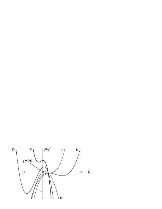
Figure 4: The plots of the polynomial $P\alpha^{3}$ for different values of ratio $\alpha=\tau/a$.

Let us consider now what condition gives the Einstein’s equations. The energy corresponding for this configuration is

$$E=-\frac{c^{4}}{2G}\int_{-\infty}^{\infty}G_{t}^{t}\,r^{2}(\rho)d\rho=-\frac{2c^{4}}{G}\left[1-\frac{15-\pi^{2}}{18}\alpha\right]a.$$ (63)

Equating this energy with zero point energy

$$E^{\rm ren}=-\frac{\hbar c}{a}f(am,\alpha,\xi)$$

we obtain the relation

$$\left[1-\frac{15-\pi^{2}}{18}\alpha\right]a^{2}=l_{P}^{2}f(am,\alpha,\xi).$$

To find parameters of stable wormholes of this kind we have to consider this equation at the minimum of function $f(am,\alpha,\xi)$. Because the function $f(am,\alpha,\xi)$ at the minimum is positive, we conclude that the stable wormhole may exist for $\alpha<18/(15-\pi^{2})=3.5$. For $\alpha=3.5$ the polynomial is equal to zero for $\xi=0.278$. Therefore the stable wormholes with this profile of throat may exist only for $\tau/a<3.5$. This upper boundary depends on the model of throat. For example, wormhole with profile of throat

$$r(\rho)=\rho\tan\frac{\rho}{\tau}+a$$

gives another boundary, namely $\tau/a<36/(\pi^{2}-6)=9.3$. Specific value of $\tau,a$ and region of $\xi$ may be found by numerical calculation of the function $f(am,\alpha,\xi)$.

VIII Conclusion

In the paper we analyzed the possibility of existence of the semi-classical wormholes with metric 1 and throat’s profile given by Eqs.2,3. Our approach consists of considering two heat kernel coefficients $B_{2}$ and $B_{3}$. We developed a method for calculation the heat kernel coefficient and obtained general expression for arbitrary coefficient in background 1. The first seven coefficients in manifest form for arbitrary profile of throat are given by Eqs. 34 and 35. The sufficient condition for existence of wormhole is positivity of both $B_{2}$ and $B_{3}$. Some additional conditions may follow from $t-t$ component of the Einstein’s equations.

The common property of both models is that the zero point energy for small size of wormhole is always positive for arbitrary constant $\xi$. This statement is opposite to that obtained for zero length throat model in Ref.KhuSus02 . The behavior of zero point energy for large size of wormhole crucially depends on the non-minimal coupling $\xi$ and parameters of the model. We show that the wormholes with the first profile of throat may be a self-consistent solution of semi-classical Einstein’s equations if the constant of non-minimal connection $\xi>0.266$. This type of wormholes is characterized by the only parameter $a$, which is the radius of wormhole’s throat. The space outside of throat polynomially tends to Minkowkian and there is no way to define the length of throat. We would like to note that the minimal connection $\xi=0$ and conformal connection $\xi=1/6$ do not obey this condition.

The second model of wormhole’s throat 3 is characterized by two parameters $\tau$ and $a$. The latter is the radius of wormhole’s throat and first is the length of throat. It is possible to introduce the length of throat because the space outside the throat becomes Minkowskian exponentially fast. Suitable illustration for this statement is Fig.4(III). The existence of this kind of wormholes crucially depends on the parameter $\xi$ and ratio of the length and radius of throat: $\alpha=\tau/a$. The general condition for $\alpha$ follows from Einstein’s equations, namely $\alpha<3.5$. The wormhole with very small parameter $\alpha$ may be self-consistent considered by scalar massive field with large value of $\xi\sim 1/\alpha$. The scalar field with conformal connection $\xi=1/6$ may self-consistently describe wormholes with $\tau/a\in(1.136,3.5)$. For $\xi=0$ we obtain another interval $\tau/a\in(1.473,3.5)$.

We would like to note that in the limit of zero length of throat $\alpha=\tau/a\to 0$ there is no connection with results of our last paper KhuSus02 where we considered wormhole with zero length of throat. The point is that the model considered in that paper is singular at the beginning. The scalar curvature is singular at throat and there is a singular surface with codimension one. For this case in Ref. GilKirVas01 the general formulas for heat kernel coefficients were obtained which can not be found as limit case of expression for smooth background ZetaBook . The reason of this lies in the following. The heat kernel coefficients are defined as an expansion of heat kernel over some dimension parameter which must be smaller then characteristic scale of background. For smooth background we may make this ratio small by taking appropriate value of expansion parameter, but singular background has at the beginning the zero value of background’s scale. This leads to new form of heat kernel coefficients. Furthermore, in the limit of large box $R\to\infty$ in this background the coefficient $B_{5/2}$ survives and it defines the behavior of energy for large size of wormhole.

Another interesting achievement of the paper is developing of the zeta-function approach Bor95 . The radial equation in this background 15 can not be solved in close form even for simple profile of throat 2. We obtain the general formula for asymptotic expansion of solutions 24, using which we find the heat kernel coefficients 34, 35 in general form. After renormalization the zero point energy may be expressed in terms of the $S$ matrix of scattering problem 44, 50. More precisely, we need only transmission coefficient $s_{11}$ of barrier 47, 51. The point is that the radial equation for massive scalar field in the background 1 looks like a one-dimensional Schrödinger equation 46 for particle with potential 47. This potential depends on both orbital momentum $l$ of particle and non-minimal coupling constant $\xi$ as well as on the radius of throat $a$ of wormhole.

In first model the domain of $\xi$ for which the energy may possess a minimum is limited from below. The reason of this is connected with the fact that the effective mass

$$m^{2}_{eff}=m^{2}+\xi\mathcal{R}=m^{2}-\frac{2\xi a^{2}}{(\rho^{2}+a^{2})^{2}}$$

may change its sign for some $\xi$ limited from below. The same situation occurs in the short-throat flat-space wormhole KhuSus02 where the scalar curvature is negative, too. This is not the case for second model. The scalar curvature in this model

$$\mathcal{R}=-\frac{6y^{2}+4\alpha-5{\alpha}^{2}+\left(4y^{2}+\alpha\left(-4+5\alpha\right)\right)\cosh(\frac{2y}{\alpha})-2y\left(-2+5\alpha\right)\sinh(\frac{2y}{\alpha})}{\tau^{2}\sinh^{4}(\frac{y}{\alpha}){\left(1-\alpha+y\coth(\frac{y}{\alpha})\right)}^{2}}$$

may change its sign depending on the parameters of model. For small $\alpha$ it is negative but starting from $\alpha=4/3$ the domain around $y=0$ appears, where the curvature becomes positive. This domain becomes larger for larger values of $\alpha$ and for $\alpha$ great enough the curvature is, in fact, positive. It is in qualitative agreement with above consideration. Indeed for small values of $\alpha$ (negative scalar curvature) we obtained low boundary for $\xi$ and vise versa, for large values of $\alpha$ (positive scalar curvature) we obtained upper boundary for $\xi$.

Appendix A

In this Appendix we reproduce in manifest form some expressions, which are rather long to reproduce them in the text. First of all let us consider the first five terms of uniform expansion

$$S^{+}(x)+S^{-}(-x) = \ln(a_{k})-\frac{1}{2}\ln(\dot{S}^{2}_{-1}r_{k}^{4})+\sum_{k=0}^{\infty}\nu^{1-2k}\int_{-x}^{+x}\dot{S}^{+}_{2k-1}dx-\ln\left\{1+\sum_{k=1}^{\infty}\nu^{-2k}\frac{\dot{S}^{+}_{2k-1}}{\dot{S}^{+}_{-1}}\right\}\allowdisplaybreaks$$

$$= \sum_{k=0}^{\infty}\nu^{1-2k}\int_{-x}^{+x}\dot{S}^{+}_{2k-1}dx+\sum_{k=0}^{\infty}\nu^{-2k}E_{2k}.$$

The coefficients with odd powers of $\nu$ read (we give the integrands, only)

$$\left[\nu^{1}\right]:\ \dot{S}_{-1}^{+} = \sqrt{1+\frac{1}{r_{k}^{2}}},\allowdisplaybreaks$$

$$\left[\nu^{-1}\right]:\ \dot{S}_{1}^{+} = -\frac{\xi\left(-1+r_{k}^{\prime 2}+2r_{k}r_{k}^{\prime\prime}\right)}{r_{k}\sqrt{1+r_{k}^{2}}}+\frac{\left(-1+r_{k}^{\prime 2}\right)+2r_{k}r_{k}^{\prime\prime}+2r_{k}^{2}\left(-1+3r_{k}^{\prime 2}\right)+6r_{k}^{3}r_{k}^{\prime\prime}-r_{k}^{4}+4r_{k}^{5}r_{k}^{\prime\prime}}{8r_{k}\left(1+r_{k}^{2}\right)^{5/2}},\allowdisplaybreaks$$

$$\left[\nu^{-3}\right]:\ \dot{S}_{3}^{+} = -\frac{\xi^{2}{\left(-1+r_{k}^{\prime 2}+2r_{k}r_{k}^{\prime\prime}\right)}^{2}}{2r_{k}\left(1+r_{k}^{2}\right)^{3/2}}-\frac{\xi}{8r_{k}\left(1+r_{k}^{2}\right)^{7/2}}\left[-\left(-1+r_{k}^{\prime 2}\right)^{2}+4r_{k}\left(1+r_{k}^{\prime 2}\right)r_{k}^{\prime\prime}\right.\allowdisplaybreaks$$

$$- \left.2r_{k}^{2}\left(1-8r_{k}^{\prime 2}+7r_{k}^{\prime}(x)^{4}-2r_{k}^{\prime\prime 2}-8r_{k}^{\prime}r_{k}^{(3)}\right)+2r_{k}^{3}\left(\left(7-31r_{k}^{\prime 2}\right)r_{k}^{\prime\prime}+2r_{k}^{(4)}\right)\right.\allowdisplaybreaks$$

$$+ \left.r_{k}^{4}\left(-1-11r_{k}^{\prime 2}+12r_{k}^{\prime 4}-4r_{k}^{\prime\prime 2}+12r_{k}^{\prime}r_{k}^{(3)}\right)+2r_{k}^{5}\left(\left(5-8r_{k}^{\prime 2}\right)r_{k}^{\prime\prime}+4r_{k}^{(4)}\right)\right.\allowdisplaybreaks$$

$$- \left.4r_{k}^{6}\left(2r_{k}^{\prime\prime 2}+r_{k}^{\prime}r_{k}^{(3)}\right)+4r_{k}^{7}r_{k}^{(4)}\right]+\frac{1}{128r_{k}\left(1+r_{k}^{2}\right)^{11/2}}\left[-\left(-1+r_{k}^{\prime 2}\right)^{2}+4r_{k}\left(1+3r_{k}^{\prime 2}\right)r_{k}^{\prime\prime}\right.\allowdisplaybreaks$$

$$+ \left.4r_{k}^{2}\left(-1+8r_{k}^{\prime 2}+9r_{k}^{\prime 4}+3r_{k}^{\prime\prime 2}+8r_{k}^{\prime}r_{k}^{(3)}\right)+4r_{k}^{3}\left(\left(7+43r_{k}^{\prime 2}\right)r_{k}^{\prime\prime}+2r_{k}^{(4)}\right)\right.\allowdisplaybreaks$$

$$+ \left.2r_{k}^{4}\left(-3+17r_{k}^{\prime 2}-294r_{k}^{\prime 4}+40r_{k}^{\prime\prime 2}+88r_{k}^{\prime}r_{k}^{(3)}\right)+r_{k}^{5}\left(4\left(15-136r_{k}^{\prime 2}\right)r_{k}^{\prime\prime}+40r_{k}^{(4)}\right)\right.\allowdisplaybreaks$$

$$+ \left.4r_{k}^{6}\left(-1-5r_{k}^{\prime 2}+120r_{k}^{\prime 4}+23r_{k}^{\prime\prime 2}+56r_{k}^{\prime}r_{k}^{(3)}\right)+4r_{k}^{7}\left(\left(13-168r_{k}^{\prime 2}\right)r_{k}^{\prime\prime}+18r_{k}^{(4)}\right)\right.\allowdisplaybreaks$$

$$- \left.r_{k}^{8}\left(1+24r_{k}^{\prime 2}+8r_{k}^{\prime\prime 2}-48r_{k}^{\prime}r_{k}^{(3)}\right)+8r_{k}^{9}\left(2\left(1+2r_{k}^{\prime 2}\right)r_{k}^{\prime\prime}+7r_{k}^{(4)}\right)-32r_{k}^{10}\left(r_{k}^{\prime\prime 2}+r_{k}^{\prime}r_{k}^{(3)}\right)+16r_{k}^{11}r_{k}^{(4)}\right],$$

and below are the coefficients with even power of $$\nu$$:

$$\left[\nu^{0}\right]:\ E_{0} = \ln(a_{k})-\frac{1}{2}\ln(\dot{S}^{2}_{-1}r_{k}^{4})\allowdisplaybreaks$$

$$\left[\nu^{-2}\right]:\ E_{2} = -\frac{\dot{S}^{+}_{1}}{\dot{S}^{+}_{-1}}.$$ (64b)

The functions $s_{p}$ are defined by relation

$$\frac{\partial}{\partial k}(S^{+}(x)+S^{-}(-x)) = \frac{\partial}{\partial k}\left\{\sum_{p=0}^{\infty}\nu^{1-2p}\int_{-kR}^{+kR}\dot{S}^{+}_{2p-1}(x)dx+\sum_{k=0}^{\infty}\nu^{-2k}E_{2k}\right\}\allowdisplaybreaks$$

$$= \sum_{p=0}^{\infty}\nu^{1-2p}\int_{-R}^{+R}s_{2p-1}(k\rho)d\rho+\sum_{p=0}^{\infty}\nu^{-2p}s_{2p}.$$

Below is the list of first four functions $s_{p}$ with odd indices, (here $r=r(\rho)$ and $z=1+k^{2}r^{2}(\rho)$)

$$s_{-1} = rz^{-1/2},\allowdisplaybreaks$$

$$s_{1} = z^{-3/2}r\left[\xi\left(-1+r^{\prime 2}+2rr^{\prime\prime}\right)+\frac{1}{8}\left\{1-4rr^{\prime\prime}\right\}\right]+z^{-5/2}\frac{3r}{4}\left[-3r^{\prime 2}+rr^{\prime\prime}\right]+z^{-7/2}\left[\frac{25}{8}rr^{\prime 2}\right],\allowdisplaybreaks$$

$$s_{3} = z^{-5/2}\frac{3r}{2}\left[\xi^{2}\left(-1+r^{\prime 2}+2rr^{\prime\prime}\right)^{2}+\xi\frac{1}{4}\left\{\left(-1+r^{\prime 2}\right)\left(1+12r^{\prime 2}\right)-2r\left(-5+8r^{\prime 2}\right)r^{\prime\prime}\right.\right.\allowdisplaybreaks$$

$$- \left.\left.4r^{2}\left(2r^{\prime\prime 2}+r^{\prime}r^{(3)}\right)+4r^{3}r^{(4)}\right\}+\frac{1}{64}\left\{1+24r^{\prime 2}-16r\left(1+2r^{\prime 2}\right)r^{\prime\prime}+32r^{2}\left(r^{\prime\prime 2}+r^{\prime}r^{(3)}\right)-16r^{3}r^{(4)}\right\}\right]\allowdisplaybreaks$$

$$+ z^{-7/2}\frac{5r}{4}\left[\xi\left\{-19\left(-1+r^{\prime 2}\right)r^{\prime 2}-3r\left(1+5r^{\prime 2}\right)r^{\prime\prime}+2r^{2}\left(3r^{\prime\prime 2}+5r^{\prime}r^{(3)}\right)\right\}\right.\allowdisplaybreaks$$

$$+ \left.\frac{1}{8}\left\{-r^{\prime 2}\left(19+120r^{\prime 2}\right)+r\left(3+200r^{\prime 2}\right)r^{\prime\prime}-2r^{2}\left(15r^{\prime\prime 2}+22r^{\prime}r^{(3)}\right)+2r^{3}r^{(4)}\right\}\right]\allowdisplaybreaks$$

$$+ z^{-9/2}\frac{175r}{8}\left[\xi r^{\prime 2}\left(-1+r^{\prime 2}+2rr^{\prime\prime}\right)+\frac{1}{200}\left\{1014r^{\prime 4}+38r^{2}r^{\prime\prime 2}+r^{\prime 2}\left(25-832rr^{\prime\prime}\right)+56r^{2}r^{\prime}r^{(3)}\right\}\right]\allowdisplaybreaks$$

$$+ z^{-11/2}\left[\frac{1989rr^{\prime 2}}{32}\left(-3r^{\prime 2}+rr^{\prime\prime}\right)\right]+z^{-13/2}\left[\frac{12155rr^{\prime 4}}{128}\right],\allowdisplaybreaks$$

$$s_{5} = z^{-7/2}\frac{5r}{2}\left[\xi^{3}\left(-1+r^{\prime 2}+2rr^{\prime\prime}\right)^{3}+\frac{\xi^{2}}{8}\left\{\left(-1+r^{\prime 2}\right)^{2}\left(3+112r^{\prime 2}\right)+12r\left(-1+r^{\prime}\right)\left(1+r^{\prime}\right)\left(4+5r^{\prime 2}\right)r^{\prime\prime}\right.\right.\allowdisplaybreaks$$ (65a)

$$- \left.\left.4r^{2}\left(-27r^{\prime\prime 2}+48r^{\prime 2}r^{\prime\prime 2}-26r^{\prime}r^{(3)}+26r^{\prime 3}r^{(3)}\right)+24r^{3}\left(-2r^{\prime\prime 3}-2r^{\prime}r^{\prime\prime}r^{(3)}-r^{(4)}+r^{\prime 2}r^{(4)}\right)\right.\right.\allowdisplaybreaks$$

$$+ \left.\left.8r^{4}\left(5r^{(3)}{}^{2}+6r^{\prime\prime}r^{(4)}\right)\right\}+\frac{\xi}{64}\left\{\left(-1+r^{\prime 2}\right)\left(3+224r^{\prime 2}+960r^{\prime 4}\right)-2r\left(-39-860r^{\prime 2}+1424r^{\prime 4}\right)r^{\prime\prime}\right.\right.\allowdisplaybreaks$$

$$+ \left.\left.8r^{2}\left(-54r^{\prime\prime 2}+186r^{\prime 2}r^{\prime\prime 2}-69r^{\prime}r^{(3)}+80r^{\prime 3}r^{(3)}\right)+8r^{3}\left(12r^{\prime\prime 3}+32r^{\prime}r^{\prime\prime}r^{(3)}+11r^{(4)}\right)\right.\right.\allowdisplaybreaks$$

$$- \left.\left.16r^{4}\left(11r^{(3)}{}^{2}+15r^{\prime\prime}r^{(4)}+3r^{\prime}r^{(5)}\right)+16r^{5}r^{(6)}\right\}+\frac{1}{512}\left\{1+112r^{\prime 2}+960r^{\prime 4}-4r\left(9+424r^{\prime 2}+192r^{\prime 4}\right)r^{\prime\prime}\right.\right.\allowdisplaybreaks$$

$$+ \left.\left.16r^{2}\left(21r^{\prime\prime 2}+106r^{\prime 2}r^{\prime\prime 2}+28r^{\prime}r^{(3)}+48r^{\prime 3}r^{(3)}\right)-64r^{3}\left(7r^{\prime\prime 3}+27r^{\prime}r^{\prime\prime}r^{(3)}+r^{(4)}+6r^{\prime 2}r^{(4)}\right)\right.\right.\allowdisplaybreaks$$

$$+ \left.\left.32r^{4}\left(9r^{(3)}{}^{2}+13r^{\prime\prime}r^{(4)}+4r^{\prime}r^{(5)}\right)-32r^{5}r^{(6)}\right\}\right]+z^{-9/2}\frac{7r}{8}\left[5\xi^{2}\left(-1+r^{\prime 2}+2rr^{\prime\prime}\right)\right.\allowdisplaybreaks$$

$$\times \left.\left(-29r^{\prime 4}+r^{\prime 2}\left(29-15rr^{\prime\prime}\right)+3rr^{\prime\prime}\left(-1+2rr^{\prime\prime}\right)+20r^{2}r^{\prime}r^{(3)}\right)+\frac{\xi}{4}\left\{-\left(-1+r^{\prime 2}\right)r^{\prime 2}\left(145+2628r^{\prime 2}\right)\right.\right.\allowdisplaybreaks$$

$$+ \left.\left.r\left(-15-2839r^{\prime 2}+2592r^{\prime 4}\right)r^{\prime\prime}+2r^{2}\left(128r^{\prime\prime 2}+643r^{\prime 2}r^{\prime\prime 2}+191r^{\prime}r^{(3)}+284r^{\prime 3}r^{(3)}\right)\right.\right.\allowdisplaybreaks$$

$$- \left.\left.2r^{3}\left(150r^{\prime\prime 3}+638r^{\prime}r^{\prime\prime}r^{(3)}+5r^{(4)}+165r^{\prime 2}r^{(4)}\right)+8r^{4}\left(7r^{(3)}{}^{2}+12r^{\prime\prime}r^{(4)}+7r^{\prime}r^{(5)}\right)\right\}\right.\allowdisplaybreaks$$

$$+ \left.\frac{1}{64}\left\{-r^{\prime 2}\left(145+5256r^{\prime 2}+20160r^{\prime 4}\right)+3r\left(5+1776r^{\prime 2}+17952r^{\prime 4}\right)r^{\prime\prime}\right.\right.\allowdisplaybreaks$$

$$- \left.\left.4r^{2}\left(113r^{\prime\prime 2}+8440r^{\prime 2}r^{\prime\prime 2}+166r^{\prime}r^{(3)}+3864r^{\prime 3}r^{(3)}\right)+4r^{3}\left(676r^{\prime\prime 3}+2816r^{\prime}r^{\prime\prime}r^{(3)}+5r^{(4)}+756r^{\prime 2}r^{(4)}\right)\right.\right.\allowdisplaybreaks$$

$$- \left.\left.8r^{4}\left(58r^{(3)}{}^{2}+93r^{\prime\prime}r^{(4)}+46r^{\prime}r^{(5)}\right)+8r^{5}r^{(6)}\right\}\right]+z^{-11/2}\frac{9r}{16}\left[175r^{\prime 2}\xi^{2}\left(-1+r^{\prime 2}+2rr^{\prime\prime}\right)^{2}\right.\allowdisplaybreaks$$

$$+ \left.\frac{\xi}{4}\left\{\left(-1+r^{\prime 2}\right)r^{\prime 2}\left(175+15054r^{\prime 2}\right)+2rr^{\prime 2}\left(4413+1976r^{\prime 2}\right)r^{\prime\prime}\right.\right.\allowdisplaybreaks$$

$$- \left.\left.14r^{2}\left(19r^{\prime\prime 2}+813r^{\prime 2}r^{\prime\prime 2}+28r^{\prime}r^{(3)}+414r^{\prime 3}r^{(3)}\right)+4r^{3}\left(133r^{\prime\prime 3}+638r^{\prime}r^{\prime\prime}r^{(3)}+221r^{\prime 2}r^{(4)}\right)\right\}\right.\allowdisplaybreaks$$

$$+ \left.\frac{1}{64}\left\{r^{\prime 2}\left(175+30108r^{\prime 2}+393408r^{\prime 4}\right)-8rr^{\prime 2}\left(2119+88298r^{\prime 2}\right)r^{\prime\prime}\right.\right.\allowdisplaybreaks$$

$$+ \left.\left.4r^{2}\left(133r^{\prime\prime 2}+65998r^{\prime 2}r^{\prime\prime 2}+196r^{\prime}r^{(3)}+31264r^{\prime 3}r^{(3)}\right)-16r^{3}\left(628r^{\prime\prime 3}+2729r^{\prime}r^{\prime\prime}r^{(3)}+791r^{\prime 2}r^{(4)}\right)\right.\right.\allowdisplaybreaks$$

$$+ \left.\left.8r^{4}\left(69r^{(3)}{}^{2}+110r^{\prime\prime}r^{(4)}+54r^{\prime}r^{(5)}\right)\right\}\right]+z^{-13/2}\frac{11r}{32}\left[221\xi r^{\prime 2}\left\{-37\left(-1+r^{\prime 2}\right)r^{\prime 2}-9r\left(1+5r^{\prime 2}\right)r^{\prime\prime}\right.\right.\allowdisplaybreaks$$

$$+ \left.\left.2r^{2}\left(9r^{\prime\prime 2}+5r^{\prime}r^{(3)}\right)\right\}+\frac{1}{8}\left\{-r^{\prime 4}\left(8177+332178r^{\prime 2}\right)+rr^{\prime 2}\left(1989+396718r^{\prime 2}\right)r^{\prime\prime}\right.\right.\allowdisplaybreaks$$

$$- \left.\left.4r^{2}r^{\prime 2}\left(21015r^{\prime\prime 2}+10168r^{\prime}r^{(3)}\right)+2r^{3}\left(631r^{\prime\prime 3}+2782r^{\prime}r^{\prime\prime}r^{(3)}+815r^{\prime 2}r^{(4)}\right)\right\}\right]\allowdisplaybreaks$$

$$+ z^{-15/2}\frac{13rr^{\prime 2}}{128}\left[12155\xi r^{\prime 2}\left(-1+r^{\prime 2}+2rr^{\prime\prime}\right)+\frac{1}{8}\left\{r^{\prime 2}\left(12155+2052348r^{\prime 2}\right)-1484372rr^{\prime 2}r^{\prime\prime}\right.\right.\allowdisplaybreaks$$

$$+ \left.\left.4r^{2}\left(34503r^{\prime\prime 2}+16880r^{\prime}r^{(3)}\right)\right\}\right]+z^{-17/2}\left[\frac{3727125rr^{\prime 4}}{512}\left(-3r^{\prime 2}+rr^{\prime\prime}\right)\right]+z^{-19/2}\left[\frac{7040125rr^{\prime 6}}{1024}\right],$$

and here is the list of first three functions $$s_{p} r=r(R) z=1+k^{2}r^{2}(R)$$ with even indices ( and )

$$s_{0} = -r^{2}z^{-1},\allowdisplaybreaks$$

$$s_{2} = -z^{-2}2r^{2}\left[\frac{1}{8}\left(1-4rr^{\prime\prime}\right)+\xi\left(-1+r^{\prime 2}+2rr^{\prime\prime}\right)\right]-z^{-3}r^{2}\left[-3r^{\prime 2}+rr^{\prime\prime}\right]-z^{-4}\left[\frac{15r^{2}r^{\prime 2}}{4}\right],\allowdisplaybreaks$$

$$s_{4} = -z^{-3}r^{2}\left[4\xi^{2}\left(-1+r^{\prime 2}+2rr^{\prime\prime}\right)^{2}+\xi\left\{\left(-1+r^{\prime 2}\right)\left(1+6r^{\prime 2}\right)-2r\left(-4+5r^{\prime 2}\right)r^{\prime\prime}-2r^{2}\left(4r^{\prime\prime 2}+r^{\prime}r^{(3)}\right)+2r^{3}r^{(4)}\right\}\right.\allowdisplaybreaks$$ (65b)

$$+ \left.\frac{1}{16}\left\{1+12r^{\prime 2}-4r\left(3+4r^{\prime 2}\right)r^{\prime\prime}+8r^{2}\left(3r^{\prime\prime 2}+2r^{\prime}r^{(3)}\right)-8r^{3}r^{(4)}\right\}\right]\allowdisplaybreaks$$

$$- z^{-4}3r^{2}\left[\xi\left(-11\left(-1+r^{\prime 2}\right)r^{\prime 2}-2r\left(1+5r^{\prime 2}\right)r^{\prime\prime}+r^{2}\left(4r^{\prime\prime 2}+5r^{\prime}r^{(3)}\right)\right)\right.\allowdisplaybreaks$$

$$+ \left.\frac{1}{8}\left\{-\left(1+4r^{\prime 2}\right)\left(-1+15r^{\prime 2}\right)+2r\left(1+53r^{\prime 2}\right)r^{\prime\prime}+r^{2}\left(-17r^{\prime\prime 2}-22r^{\prime}r^{(3)}\right)+r^{3}r^{(4)}\right\}\right]\allowdisplaybreaks$$

$$- z^{-5}r^{2}\left[30\xi r^{\prime 2}\left(-1+r^{\prime 2}+2rr^{\prime\prime}\right)+\frac{1}{4}\left\{3r^{\prime 2}\left(5+172r^{\prime 2}\right)-432rr^{\prime 2}r^{\prime\prime}+4r^{2}\left(5r^{\prime\prime 2}+7r^{\prime}r^{(3)}\right)\right\}\right]\allowdisplaybreaks$$

$$- z^{-6}\left[\frac{565r^{2}r^{\prime 2}}{8}\left(-3r^{\prime 2}+rr^{\prime\prime}\right)\right]-z^{-7}\left[\frac{1695r^{2}r^{\prime 4}}{16}\right].$$

Below are the functions $\omega_{a},\ \omega_{b}$ and $\omega_{c}$ with definitions of the corresponding integrals.

$$\omega_{a} = \pi^{2}\left[-\frac{2}{3}a+32a^{3}\int_{0}^{1}\frac{d\nu\nu}{e^{2\pi\nu a}+1}\left(\sqrt{1-\nu^{2}}+\nu^{2}\ln\left[\frac{\nu}{1+\sqrt{1-\nu^{2}}}\right]\right)\right],\allowdisplaybreaks$$

$$\omega_{b} = -\frac{5}{3}\pi^{4}a^{2}+a\pi^{2}\left[-16(\gamma+2\ln 2)\xi+\frac{4}{3}(3+2\gamma)\right]-8\pi^{2}a\ln(2a)(1-\tanh(\pi a))(1-2\xi)\allowdisplaybreaks$$

$$- 32\pi^{2}a\xi V_{1}+\frac{4}{3}\pi^{2}a[V_{1}+6V_{2}-4\pi aV_{3}+2\pi aV_{4}-5\pi^{2}a^{2}V_{5}],\allowdisplaybreaks$$

$$\omega_{c} = U_{1}+U_{2}+U_{3}+U_{4}+U_{5}+U_{6}.$$ (66)

Here we introduced five functions for $\omega_{b}$

$$V_{1} = \frac{\pi a}{2}\int_{0}^{1}\frac{\ln(2a\nu)}{\cosh^{2}(\pi a\nu)}d\nu-\int_{0}^{1}\frac{\nu d\nu}{e^{2\pi a\nu}+1}\left[\ln\left(\frac{\nu}{1+\sqrt{1-\nu^{2}}}\right)+\frac{1}{1+\sqrt{1-\nu^{2}}}\right],\allowdisplaybreaks$$

$$V_{2} = \int_{0}^{1}\frac{\nu d\nu}{e^{2\pi a\nu}+1}\ln\left(\frac{\nu}{1+\sqrt{1-\nu^{2}}}\right),\allowdisplaybreaks$$

$$V_{3} = \int_{0}^{1}\frac{d\nu}{\cosh^{2}(\pi a\nu)}\ln\left(\frac{\nu}{1+\sqrt{1-\nu^{2}}}\right),\allowdisplaybreaks$$

$$V_{4} = \int_{0}^{1}\frac{d\nu\sqrt{1-\nu^{2}}}{\cosh^{2}(\pi a\nu)},\allowdisplaybreaks$$

$$V_{5} = \int_{0}^{1}\frac{\sinh(\pi a\nu)d\nu}{\cosh^{2}(\pi a\nu)}\left[\nu\sqrt{1-\nu^{2}}-\arccos\nu\right],$$

and six for $\omega_{c}$

$$U_{1} = -\frac{229\pi^{4}}{2520}-\pi a\int_{0}^{1}f_{1}(a\nu)\arccos\nu d\nu,\allowdisplaybreaks$$

$$U_{2} = \pi a\int_{1}^{\infty}f_{3}(a\nu)\frac{d\nu}{\nu}+\pi a\int_{0}^{1}\frac{f_{3}(a\nu)\nu d\nu}{1+\sqrt{1-\nu^{2}}},\allowdisplaybreaks$$

$$U_{3} = \pi a\int_{1}^{\infty}f_{5}(a\nu)\frac{d\nu}{\nu}\left(\frac{1}{2}+\frac{1}{3\nu^{2}}\right)+\frac{\pi}{3}a\int_{0}^{1}f_{5}(a\nu)\nu d\nu\left[\frac{2}{1+\sqrt{1-\nu^{2}}}+\frac{1}{2(1+\sqrt{1-\nu^{2}})^{2}}\right],\allowdisplaybreaks$$

$$U_{4} = \frac{\pi^{2}}{2}\int_{0}^{1}\frac{f_{2}d\nu}{\cosh^{2}(\pi a\nu)}\ln\left(\frac{\nu}{1+\sqrt{1-\nu^{2}}}\right),\allowdisplaybreaks$$

$$U_{5} = \frac{\pi^{2}}{4}\int_{1}^{\infty}\frac{f_{4}d\nu}{\nu^{2}\cosh^{2}(\pi a\nu)}+\frac{\pi^{2}}{4}\int_{0}^{1}\frac{f_{4}d\nu}{\cosh^{2}(\pi a\nu)}\left[\ln\left(\frac{\nu}{1+\sqrt{1-\nu^{2}}}\right)+\frac{\nu}{1+\sqrt{1-\nu^{2}}}\right],\allowdisplaybreaks$$

$$U_{5} = \frac{\pi^{2}}{8}\int_{1}^{\infty}\frac{f_{6}(\nu^{2}+1)d\nu}{\nu^{4}\cosh^{2}(\pi a\nu)}+\frac{3\pi^{2}}{16}\int_{0}^{1}\frac{f_{6}d\nu}{\cosh^{2}(\pi a\nu)}\left[\ln\left(\frac{\nu}{1+\sqrt{1-\nu^{2}}}\right)+\frac{\nu}{1+\sqrt{1-\nu^{2}}}+\frac{1}{3}\frac{\nu}{(1+\sqrt{1-\nu^{2}})^{2}}\right],$$

where

$$f_{1}(\nu) = \frac{4\pi}{315}(14595\Pi_{2}(\nu)-43638\Pi_{3}(\nu)+47736\Pi_{4}(\nu)-17680\Pi_{5}(\nu)),\allowdisplaybreaks$$

$$f_{3}(\nu) = \frac{32\pi\xi}{3}(29\Pi_{2}(\nu)-10\Pi_{3}(\nu))-\frac{8\pi}{315}(32445\Pi_{2}(\nu)-64113\Pi_{3}(\nu)+55692\Pi_{4}(\nu)-17680\Pi_{5}(\nu)),\allowdisplaybreaks$$

$$f_{5}(\nu) = -\frac{64\pi\xi}{3}(16\Pi_{2}(\nu)-5\Pi_{3}(\nu))+\frac{32\pi}{315}(6720\Pi_{2}(\nu)-10773\Pi_{3}(\nu)+7956\Pi_{4}(\nu)-2210\Pi_{5}(\nu)),\allowdisplaybreaks$$

$$f_{2}(\nu) = -\frac{229\pi}{630},\allowdisplaybreaks$$

$$f_{4}(\nu) = \frac{376\pi}{3}\xi-\frac{5948\pi}{315},\allowdisplaybreaks$$

$$f_{6}(\nu) = 32\pi\xi^{2}-\frac{544\pi}{3}\xi+\frac{8824\pi}{315},$$

and

$$\Pi_{2}(\nu) = \frac{\pi^{2}}{2}Sc(\nu),\allowdisplaybreaks$$

$$\Pi_{3}(\nu) = \pi^{2}(Sc(\nu)+\frac{1}{8}\nu Sc^{\prime}(\nu)),\allowdisplaybreaks$$

$$\Pi_{4}(\nu) = \pi^{2}(\frac{3}{2}Sc(\nu)+\frac{17}{48}\nu Sc^{\prime}(\nu)+\frac{1}{48}\nu^{2}Sc^{\prime\prime}(\nu)),\allowdisplaybreaks$$

$$\Pi_{5}(\nu) = \pi^{2}(2Sc(\nu)+\frac{259}{384}\nu Sc^{\prime}(\nu)+\frac{29}{384}\nu^{2}Sc^{\prime\prime}(\nu))+\frac{1}{384}\nu^{3}Sc^{\prime\prime\prime}(\nu)),\allowdisplaybreaks$$

$$Sc(\nu) = \frac{\sinh(\pi a\nu)}{\cosh^{3}(\pi a\nu)}.$$

References

• (1) E. R. Bezerra de Mello, V. B. Bezerra and N. R. Khusnutdinov, J. Math. Phys. 42, 562 (2001).
• (2) M. Bordag, J. Phys. A 28, 755 (1995); M. Bordag and K. Kirsten, Phys. Rev. D 53, 5753 (1996); M. Bordag, K. Kirsten, and E. Elizalde, J. Math. Phys. 37, 895 (1996); M. Bordag, E. Elizalde, K. Kirsten, and S. Leseduarte, Phys. Rev. D 56, 4896 (1997); M. Bordag, K. Kirsten, and D. Vassilevich, Phys. Rev. D 59, 085011 (1999).
• (3) A. Einstein and N. Rosen, Phys. Rev. 48, 73 (1935).
• (4) E. Elizalde, S. D. Odintsov, A. Romeo, A. A. Bytsenko, and S. Zerbini, Zeta Regularization Techniques with Applications, (World Scientific, Singapore, 1994).
• (5) J. S. Dowker and R. Critchley, Phys. Rev. D 13, 3224 (1976); W. Hawking, Commun. Math. Phys. 55, 133 (1977); S. K. Blau, M. Visser, and A. Wipf, Nucl. Phys. B 310, 163 (1988).
• (6) L. Flamm, Phys. Z., 17, 48 (1916).
• (7) D. V. Fursaev, Phys. Lett. B 334, 53 (1994).
• (8) P. B. Gilkey, K. Kirsten and D. V. Vassilevich, Nucl. Phys. B 601, 125 (2001).
• (9) S. W. Hawking and G. F. R. Ellis, The Large Scale Structure of Space-Time, (Cambridge University Press, Cambridge, London, 1973).
• (10) N. R. Khusnutdinov and M. Bordag, Phys. Rev. D 59, 064017 (1999).
• (11) N. R. Khusnutdinov and S. V. Sushkov, Phys. Rev. D 65, 084028 (2002).
• (12) M. S. Morris and K. S. Thorne, Am. J. Phys. 56, 395 (1988).
• (13) M. S. Morris, K. S. Thorne and U. Yurtsever, Phys. Rev. Lett. 61, 1446 (1988).
• (14) S. V. Sushkov, Phys. Lett. A 164, 33 (1992); D. Hochberg, A. Popov, S. V. Sushkov, Phys. Rev. Lett. 78, 2050 (1997).
• (15) S. V. Sushkov, Grav. & Cosmol. 7, 194 (2001)
• (16) M. Visser, Lorentzian Wormholes: from Einstein to Hawking,(American Institute of Physics, Woodbury, 1995).
• (17) J. A. Wheeler, Phys. Rev. 97, 511 (1955).