One-dimensional topologically nontrivial
solutions in the Skyrme model

Abstract

We consider the Skyrme model using the explicit parameterization of the rotation group ${\mathbb{S}}{\mathbb{O}}(3)$ through elements of its algebra. Topologically nontrivial solutions already arise in the one-dimensional case because the fundamental group of ${\mathbb{S}}{\mathbb{O}}(3)$ is ${\mathbb{Z}}_{2}$. We explicitly find and analyze one-dimensional static solutions. Among them, there are topologically nontrivial solutions with finite energy. We propose a new class of projective models whose target spaces are arbitrary real projective spaces ${\mathbb{R}}{\mathbb{P}}^{d}$.

1 Introduction

The Skyrme model [1] is one of the fundamental contemporary mathematical physics models, and it finds applications in different fields of physics ranging from the theory of elementary particles to solid state physics. The model was originally proposed in terms of four scalar fields taking values on the three-dimensional sphere ${\mathbb{S}}^{3}$. The Lagrangian of the model was also written in terms of elements of the algebra $\mathfrak{s}\mathfrak{u}(2)$ because the sphere ${\mathbb{S}}^{3}$ is diffeomorphic to the group ${\mathbb{S}}{\mathbb{U}}(2)$ as a manifold. Because the fundamental and the second homotopy groups of unitary groups ${\mathbb{S}}{\mathbb{U}}(n)$, $n\geq 2$, and spheres ${\mathbb{S}}^{n}$, $n\geq 3$, are trivial, one- and two-dimensional topologically nontrivial solutions of the corresponding models do not exist. In such a parameterization of the Skyrme model, topologically nontrivial solutions are related to the third homotopy group $\pi_{3}({\mathbb{S}}^{3})={\mathbb{Z}}$. But these solutions have not yet been found in explicit form.

In subsequent years, much attention was also given to ${\mathbb{S}}{\mathbb{O}}(n)$ models where target spaces are any dimensional spheres ${\mathbb{S}}^{n-1}$ with the rotation groups ${\mathbb{S}}{\mathbb{O}}(n)$ being the symmetry groups. Reviews of these models and references can be found in [2–6]. In what follows, we call these models ${\mathbb{S}}^{n}$ models preserving the term ${\mathbb{S}}{\mathbb{O}}(n)$ model for the case where the target space is the group manifold itself.

Topological solitons of the lowest dimension exist for ${\mathbb{S}}^{1}$ models for which $\pi({\mathbb{S}}^{1})={\mathbb{Z}}$. For example, there are well known kinks in the sine–Gordon model. Topologically nontrivial solutions for higher homotopy groups appear in the ${\mathbb{S}}^{2}$ model, where the second homotopy group is nontrivial, $\pi_{2}({\mathbb{S}}^{2})={\mathbb{Z}}$. The corresponding static solutions with nontrivial topological charge were found and analyzed in [7].

As already noted, the Lagrangian for the Skyrme model can be written in terms of the $\mathfrak{s}\mathfrak{u}(2)$ algebra elements. Because the algebras for the ${\mathbb{S}}{\mathbb{U}}(2)$ and ${\mathbb{S}}{\mathbb{O}}(3)$ groups are isomorphic, the Skyrme model can be considered the ${\mathbb{S}}{\mathbb{O}}(3)$ model with the group manifold itself being the target space. For this, we use the known (see, i.g., [8]), but not widely used, explicit parameterization of the rotation group ${\mathbb{S}}{\mathbb{O}}(3)$, i.e., we work with the three-dimensional group manifold directly. Topologically nontrivial solutions appear here, even in the one-dimensional case, because the fundamental group of the rotation group ${\mathbb{S}}{\mathbb{O}}(3)$ is nontrivial $(\pi({\mathbb{S}}{\mathbb{O}}(3))={\mathbb{Z}}_{2})$. We explicitly find the corresponding static solutions. They are analyzed and compared with the static solutions of the ${\mathbb{S}}^{2}$ model.

The explicit parameterization of the group ${\mathbb{S}}{\mathbb{O}}(3)$ used in this paper allows a generalization. It is well known that the ${\mathbb{S}}{\mathbb{O}}(3)$ group manifold is diffeomorphic to the three-dimensional projective space ${\mathbb{R}}{\mathbb{P}}^{3}$ (see, e.g., [9]). This allows generalizing the Skyrme model to the case of arbitrary projective spaces over the field of real numbers where the target space is an arbitrary projective space ${\mathbb{R}}{\mathbb{P}}^{n}={\mathbb{S}}^{n}/{\mathbb{Z}}_{2}$. The projective space ${\mathbb{R}}{\mathbb{P}}^{n}$ can be parameterized by points in the Euclidean space $\{\omega^{i}\}\in{\mathbb{R}}^{n}$, $i=1,\dotsc,n$, inside the ball $\omega=\sqrt{\omega^{i}\omega_{i}}\leq\pi$ for which the antipodal points of the boundary sphere of radius $\pi$ are identified. In this parameterization of the projective space, the Lagrangian for an ${\mathbb{R}}{\mathbb{P}}^{n}$ model depends on $n$ fields $\omega^{i}(x)$, and is invariant under local discrete transformations $\omega^{i}\rightarrow\omega^{i}+2\pi\omega^{i}/\omega$. In contrast to gauge models, the symmetry group at each point of a space-time is a discreet group ${\mathbb{Z}}$ of translations on a constant vector, not a Lie group. Representation of the translation group is local and depends on the space-time point because the direction of a vector changes continuously.

We start our consideration by describing the explicit parameterization of the group ${\mathbb{O}}(3)$. In Secs. 3, 4, and 5 we write the respective Lagrangian for ${\mathbb{S}}{\mathbb{O}}(3)$, ${\mathbb{S}}{\mathbb{U}}(2)$, and ${\mathbb{S}}^{2}$ models, and we compare them. Static solutions for the ${\mathbb{S}}^{2}$ and ${\mathbb{S}}{\mathbb{O}}(3)$ models are found and compared in Secs. 6 and 7. The ${\mathbb{S}}{\mathbb{O}}(3)$ model is generalized to arbitrary real projective spaces ${\mathbb{R}}{\mathbb{P}}^{d}$ in Sec. 8.

2 Parameterization of three-dimensional
rotation group

Calculations for the group ${\mathbb{O}}(3)$ can be conveniently performed in the explicit parameterization of group elements by elements of its algebra. An element of the algebra $\mathfrak{s}\mathfrak{o}(3)$ can be parameterized by an arbitrary antisymmetric $3\times 3$ matrix

$$(\omega\varepsilon)_{i}{}^{j}=(\omega^{k}\varepsilon_{k})_{i}{}^{j}=\omega^{k}\varepsilon_{ki}{}^{j}~{}~{}\in\mathfrak{s}\mathfrak{o}(3),$$ (1)

where $\varepsilon_{ijk}$ is the totally antisymmetric third rank tensor, $\varepsilon_{123}=1$, and raising and lowering of indices is performed with the Kronecker symbol. Here, the first index $k$ enumerates the basis of the algebra, and the indices $i$ and $j$ are considered matrix indices. An algebra element is parameterized by a three-dimensional vector $\omega^{k}\in{\mathbb{R}}^{3}$, and the ${\mathbb{O}}(3)$ group is therefore three-dimensional. There is a single element of the group ${\mathbb{S}}{\mathbb{O}}(3)$ (from the component connected to the unity element) that corresponds to an element of the algebra:

$$S_{(+)i}{}^{j}=(e^{(\omega\varepsilon)})_{i}{}^{j}=\delta_{i}^{j}{\sf\,cos\,}\omega\ +\frac{(\omega\varepsilon)_{i}{}^{j}}{\omega}{\sf\,sin\,}\omega+\frac{\omega_{i}\omega^{j}}{\omega^{2}}(1-{\sf\,cos\,}\omega)~{}\in{\mathbb{S}}{\mathbb{O}}(3),$$ (2)

where $\omega=\sqrt{\omega^{i}\omega_{i}}$ is the modulus of the vector $\omega^{i}$. Direct calculations show that $S_{(+)i}{}^{j}$ is indeed the orthogonal matrix. Vice versa, any orthogonal matrix with a positive determinant can be represented in form (2) for a vector $\omega^{i}$. We note that in contrast to the algebra element, the group element has both symmetric and antisymmetric parts. It can be verified that the ${\mathbb{S}}{\mathbb{O}}(3)$-group element is invariant with respect to translation of a vector $\omega^{i}\rightarrow\omega^{i}+2\pi\omega^{i}/\omega$,

$$S_{(+)i}{}^{j}\left(\omega^{k}+2\pi\frac{\omega^{k}}{\omega}\right)=S_{(+)i}{}^{j}(\omega^{k}),$$

and this is the only invariance. The shift of the vector $\omega^{i}$ changes only its length $\omega\rightarrow\omega+2\pi$, leaving its direction unchanged. It is easy to observe the symmetry of the rotation matrix by noting that the ratio $\omega^{i}/\omega$ defining the direction of vector $\omega^{i}$ remains unchanged under an arbitrary shift,

$$\frac{\omega^{i}}{\omega}\rightarrow\frac{\omega^{i}+c\omega^{i}/\omega}{\omega+c}=\frac{\omega^{i}}{\omega},~{}~{}~{}~{}c\in{\mathbb{R}}.$$

An element of the rotation group is therefore parameterized by a point of the Euclidean space $\omega^{i}\in{\mathbb{R}}^{3}$ with the only equivalence relation

$$\omega^{i}\approx\omega^{i}+2\pi\frac{\omega^{i}}{\omega}.$$ (3)

Here, the uncertainty at zero is resolved along radial directions $\omega^{i}=\epsilon k^{i}$, $\epsilon\to 0$. The origin of the coordinate system is thus identified with the spheres of radii $2\pi m$, $m=1,2,\dotsc$.

The vector $\omega^{i}$ parameterizes the ${\mathbb{S}}{\mathbb{O}}(3)$ as follows. The direction of $\omega^{i}$ coincides with the rotation axis, and its modulus $\omega$ equals the rotation angle. Each ${\mathbb{S}}{\mathbb{O}}(3)$-group element is then identified with a point of the three-dimensional ball ${\mathbb{B}}^{3}_{\pi}$ having the radius $\pi$ and the center at the origin. Different rotations correspond to different points, and the antipodal points of the boundary sphere must be identified because rotations through the angles $\pi$ and $-\pi$ about a fixed axis yield the same result.

The full group of three-dimensional rotations ${\mathbb{O}}(3)$ consists of two disconnected components: orthogonal matrices with positive $S_{(+)}$ and negative $S_{(-)}$ determinants. Elements of the full group ${\mathbb{O}}(3)$ are parameterized, for example, by algebra elements (1) as

$$S_{(\pm)i}{}^{j}=\delta_{i}^{j}{\sf\,cos\,}\omega+\frac{(\omega\varepsilon)_{i}{}^{j}}{\omega}{\sf\,sin\,}\omega+\frac{\omega_{i}\omega^{j}}{\omega^{2}}(\pm 1-{\sf\,cos\,}\omega)~{}\in{\mathbb{O}}(3),$$ (4)

We note that there are two group elements $S_{(\pm)}\in{\mathbb{O}}(3)$, one from each component, which correspond to an element of the algebra $(\omega\varepsilon)_{i}{}^{j}\in\mathfrak{s}\mathfrak{o}(3)$.

The inverse matrices have the form

$$S^{-1}_{(\pm)i}{}^{j}(\omega^{k})=S_{(\pm)i}{}^{j}(-\omega^{k})=\delta_{i}^{j}{\sf\,cos\,}\omega-\frac{(\omega\varepsilon)_{i}{}^{j}}{\omega}{\sf\,sin\,}\omega+\frac{\omega_{i}\omega^{j}}{\omega^{2}}(\pm 1-{\sf\,cos\,}\omega)~{}\in{\mathbb{O}}(3),$$ (5)

i.e., they correspond to the inverse vector $-\omega^{i}\in{\mathbb{R}}^{3}$. In other words, the inverse group element corresponds to the rotation of the Euclidean space about the same axis through the opposite angle.

Contraction of the matrix $S_{(\pm)i}{}^{j}$ with the vector $\omega_{j}$ yields

$$S_{(\pm)i}{}^{j}\omega_{j}=\pm\omega_{i}.$$

This means that the vector $\omega^{i}$ is the eigenvector of orthogonal matrices with the eigenvalues $\pm 1$. In other words, rotations $S_{(+)}$ leave the direction of the rotation axis unchanged, while rotations $S_{(-)}$ change it to the opposite direction.

We assume that ${\mathbb{O}}(3)$-group element depends smoothly on a point of an arbitrary manifold ${\mathbb{M}}$, i.e.,

$$\omega^{i}(x):~{}~{}{\mathbb{M}}\rightarrow{\mathbb{O}}(3).$$

We introduce the notation

$$l_{(\pm)\alpha i}{}^{j}=(\partial_{\alpha}S_{(\pm)}^{-1}S_{(\pm)})_{i}{}^{j}.$$ (6)

The validity of the formula

$$\begin{split}l_{(\pm)\alpha i}{}^{j}=\mp\frac{(\partial_{\alpha}\omega\varepsilon)_{i}{}^{j}}{\omega}{\sf\,sin\,}\omega-\frac{\partial_{\alpha}\omega(\omega\varepsilon)_{i}{}^{j}}{\omega}\left(1\mp\frac{{\sf\,sin\,}\omega}{\omega}\right)&\\ \pm\frac{\partial_{\alpha}\omega_{i}\omega^{j}-\omega_{i}\partial_{\alpha}\omega^{j}}{\omega^{2}}(\pm 1-{\sf\,cos\,}\omega)&~{}~{}\in\mathfrak{s}\mathfrak{o}(3)\end{split}$$ (7)

can be shown by straightforward calculations. This matrix is antisymmetric with respect to its indices and is hence an element of the algebra $\mathfrak{s}\mathfrak{o}(3)$. It is the trivial ${\mathbb{O}}(3)$ connection (pure gauge) for which the curvature tensor is zero. The trivial ${\mathbb{S}}{\mathbb{O}}(3)$ connection is denoted by $l_{\alpha i}{}^{j}=l_{(+)\alpha i}{}^{j}$ in what follows.

The considered parameterization of the rotation group shows that the group manifold is compact and orientable. The component ${\mathbb{S}}{\mathbb{O}}(3)$ connected to the unity element, as a manifold, is diffeomorphic to the three-dimensional projective space ${\mathbb{R}}{\mathbb{P}}^{3}$. It is not simply connected, and its fundamental group is ${\mathbb{Z}}_{2}$.

3 The Lagrangian for the Skyrme model

We consider the $n$-dimensional Minkowski space ${\mathbb{R}}^{1,n-1}$ with Cartesian coordinates $x^{\alpha}$, $\alpha=0,1,\dotsc,n-1$. Let an element of the rotation group $\omega^{i}(x)$ be given at each point of the Minkowski space. To describe $\pi$-mesons Skyrme proposed the action [1]

$$S=\int dxL=\int dx\left(-\frac{\varrho}{4}{\sf\,tr\,}(l_{\alpha}l^{\alpha})-\frac{\kappa}{8}{\sf\,tr\,}([l_{\alpha},l_{\beta}][l^{\alpha},l^{\beta}])\right),$$ (8)

where $\varrho$ and $\kappa$ are coupling constants and square brackets denote the matrix commutator. Skyrme considered $l_{\alpha}$ as a trivial ${\mathbb{S}}{\mathbb{U}}(2)$ connection and parameterized it by a four-vector in the isotopic space with the four-vector taking values on a three-dimensional sphere ${\mathbb{S}}^{3}$, i.e., he considered action (8) as the ${\mathbb{S}}{\mathbb{U}}(2)$ model or, equivalently, as the ${\mathbb{S}}^{3}$ model. We consider (8) as the action for the ${\mathbb{S}}{\mathbb{O}}(3)$ model using the parameterization of the rotation group from the previous section. We note that these models are not equivalent. Substituting the explicit expression for $l_{\alpha}$ in terms of the group parameters (7) yields the Lagrangian for three independent scalar fields $\omega^{i}$,

$$\begin{split}L&=\varrho\left(\frac{1}{2}\partial_{\alpha}\omega^{2}+(1-{\sf\,cos\,}\omega)\frac{(\partial_{\alpha}\omega\partial_{\alpha}\omega)-\partial_{\alpha}\omega^{2}}{\omega^{2}}\right)\\ &+\kappa\left((1-{\sf\,cos\,}\omega)\frac{(\partial_{\alpha}\omega\partial_{\alpha}\omega)\partial_{\beta}\omega^{2}-(\partial_{\alpha}\omega\partial_{\beta}\omega)\partial_{\alpha}\omega\partial_{\beta}\omega}{\omega^{2}}\right.\\ &+\left.(1-{\sf\,cos\,}\omega)^{2}\frac{(\partial_{\alpha}\omega\partial_{\alpha}\omega)^{2}-(\partial_{\alpha}\omega\partial_{\beta}\omega)^{2}-2(\partial_{\alpha}\omega\partial_{\alpha}\omega)\partial_{\beta}\omega^{2}+2(\partial_{\alpha}\omega\partial_{\beta}\omega)\partial_{\alpha}\omega\partial_{\beta}\omega}{\omega^{4}}\right),\end{split}$$ (9)

where we introduce the notation for the scalar product

$$(\partial_{\alpha}\omega\partial_{\alpha}\omega)=\partial_{\alpha}\omega^{i}\partial_{\alpha}\omega_{i}\neq\partial_{\alpha}\omega^{2}.$$

In this expression, repeated Greek indices imply summation with the Minkowski metric tensor$\eta_{\alpha\beta}$, and we do not distinguish lower and upper indices for simplicity. The three fields $\omega^{i}(x)$ in the Lagrangian are independent dynamical variables free of constraints except equivalence relation (3). These fields are scalars under coordinate transformations in the Minkowski space ${\mathbb{R}}^{1,n-1}$ and vector components under global rotations of the Euclidean target-space ${\mathbb{R}}^{3}$. It can be verified that Lagrangian (9) is invariant under the Poicaré group acting in the Minkowski space, global ${\mathbb{O}}(3)$ rotations acting in the target space $\omega^{i}\in{\mathbb{R}}^{3}$, and local translations (3). The latter transformation implies that the length of the vector $\omega^{i}\in{\mathbb{R}}^{3}$ at each point $x\in{\mathbb{R}}^{1,n-1}$ can be changed by a constant value divisible by $2\pi$. At the same time, this discrete transformation is local because the direction of the vector $\omega^{i}$ changes from point to point. By virtue of this invariance, we assume a vector $\omega^{i}$ to take values inside the ball of radius $\pi$ with the center at the origin of the target space $\omega^{i}\in{\mathbb{B}}^{3}_{\pi}\subset{\mathbb{R}}^{3}$.

To analyze the Skyrme model in form (9), it is convenient to consider four new variables: the length of the vector $\omega^{i}$ (the rotation angle $\omega$) and its direction (the rotation axis $k^{i}$), not the vector $\omega^{i}$ itself

$$\omega=\sqrt{(\omega^{1})^{2}+(\omega^{2})^{2}+(\omega^{3})^{2}},~{}~{}~{}~{}k^{i}=\frac{\omega^{i}}{\omega}.$$ (10)

By definition, the vector $k^{i}$ has unit length $(k,k)=k^{i}k_{i}=1$. In terms of the new variables, Lagrangian (9) becomes

$$\begin{split}L&=\varrho\left(\frac{1}{2}\partial_{\alpha}\omega^{2}+(1-{\sf\,cos\,}\omega)(\partial_{\alpha}k\partial_{\alpha}k)\right)\\ &+\kappa\left(\vphantom{\frac{1}{2}}(1-{\sf\,cos\,}\omega)\left[(\partial_{\alpha}k\partial_{\alpha}k)\partial_{\beta}\omega^{2}-(\partial_{\alpha}k\partial_{\beta}k)\partial_{\alpha}\omega\partial_{\beta}\omega\right]\right.\\ &\left.\vphantom{\frac{1}{2}}~{}~{}~{}~{}~{}~{}~{}~{}~{}~{}~{}~{}~{}~{}~{}+(1-{\sf\,cos\,}\omega)^{2}\left[(\partial_{\alpha}k\partial_{\alpha}k)^{2}-(\partial_{\alpha}k\partial_{\beta}k)^{2}\right]\right).\end{split}$$ (11)

We recall that $(\partial_{\alpha}k\partial_{\alpha}k)=\partial_{\alpha}k^{i}\partial_{\alpha}k_{i}$. Transformation (3) changes only the length of a vector

$$\omega\rightarrow\omega+2\pi,~{}~{}~{}~{}k^{i}\rightarrow k^{i}.$$ (12)

The invariance of Lagrangian (11) under transformations (12) follows immediately. Moreover, each of its terms is separately invariant.

4 Comparison with the ${\mathbb{S}}{\mathbb{U}}(2)$ model

The form of the action of Skyrme model (8) for group parameters depends only on an algebra, and not on the group that represents the target space. To show the dependence of the model on the group, we consider the ${\mathbb{S}}{\mathbb{U}}(2)$ model. An element of the algebra $\mathfrak{s}\mathfrak{u}(2)$ has the form

$$\omega^{k}\frac{i}{2}(\sigma_{k})_{\textsc{a}}{}^{\textsc{b}}~{}\in\mathfrak{s}\mathfrak{u}(2),~{}~{}~{}~{}{\textsc{a}},{\textsc{b}}=1,2,$$

where $\sigma_{k}$ are the Pauli matrices. We introduce the factor $i/2$ for the commutators of the basis vectors for the algebras $\mathfrak{s}\mathfrak{u}(2)$ and $\mathfrak{s}\mathfrak{o}(3)$ to have the same form. The corresponding ${\mathbb{S}}{\mathbb{U}}(2)$ group element is

$$U_{\textsc{a}}{}^{\textsc{b}}=(e^{(i\omega\sigma/2)})_{\textsc{a}}{}^{\textsc{b}}=\delta_{\textsc{a}}^{\textsc{b}}{\sf\,cos\,}\frac{\omega}{2}+i\frac{\omega^{k}\sigma_{k{\textsc{a}}}{}^{\textsc{b}}}{\omega}{\sf\,sin\,}\frac{\omega}{2}~{}~{}\in{\mathbb{S}}{\mathbb{U}}(2).$$ (13)

From this expression for a group element, we obtain the identity

$$U_{\textsc{a}}{}^{\textsc{b}}\left(\omega^{i}+4\pi\frac{\omega^{i}}{\omega}\right)=U_{\textsc{a}}{}^{\textsc{b}}(\omega^{i}),$$

i.e., there exists the equivalence relation

$$\omega^{i}\approx\omega^{i}+4\pi\frac{\omega^{i}}{\omega}$$ (14)

in the parameter space for the group ${\mathbb{S}}{\mathbb{U}}(2)$. In comparison with equivalence relation (3) for ${\mathbb{S}}{\mathbb{O}}(3)$, the shift is performed by a vector having a double length. This means that the group manifold is parameterized by internal points of the ball ${\mathbb{B}}^{3}_{2\pi}$ of radius $2\pi$. Moreover, all points of the boundary sphere must be identified. This is the second equivalence relation in the parameter space,

$$\omega_{1}^{i}|_{\omega_{1}=2\pi}\approx\omega_{2}^{i}|_{\omega_{2}=2\pi}.$$ (15)

The extra equivalence relation is due to the absence of the third term in (13) as compared with (2). It is another difference from the rotation-group case, where only antipodal points on the boundary sphere are identified, which is taken into account in equivalence relation (3). It can be shown that there are no other equivalence relations in the parameter space except (14) and (15).

It can be easily verified that the Lagrangian for the Skyrme model has the same form (11) for both the groups ${\mathbb{S}}{\mathbb{U}}(2)$ and ${\mathbb{S}}{\mathbb{O}}(3)$. The difference amounts to equivalence relations (3) and (14) and identifications of points on boundary sphere (15). The last property results in the difference in fundamental groups leading to the existence of one-dimensional topologically nontrivial solutions in the ${\mathbb{S}}{\mathbb{O}}(3)$ Skyrme model.

5 ${\mathbb{S}}^{2}$ model

The ${\mathbb{S}}^{2}$ model has attracted much interest for many years. Because both the ${\mathbb{S}}{\mathbb{O}}(3)$ Skyrme model and ${\mathbb{S}}^{2}$ model are described by three-dimensional vectors, and any vector of a fixed length can be represented as a result of action of the rotation matrix on some fixed vector of the same length, there arises a question about a possible relation between these models. In spite of the nonequivalence of these models, there is a relation between them, which we consider in this section.

We relate the ${\mathbb{S}}{\mathbb{O}}(3)$ in Sec. 3 to the ${\mathbb{S}}^{2}$ model. Given a unit vector $n^{i}(x)$, $(n,n)=1$, at each point of the Minkowski space ${\mathbb{R}}^{1,n-1}$, we obtain the target space, which is the two-dimensional sphere ${\mathbb{S}}^{2}$. We let the capital letters $X,Y$, and $Z$ denote the Cartesian coordinates of the target space. We consider the Lagrangian proposed by Faddeev for the ${\mathbb{S}}^{2}$ model [10]

$$\begin{split}L_{\mathrm{F}}&=m^{2}(\partial_{\alpha}n\partial_{\alpha}n)+\frac{1}{e^{2}}(n^{i}\varepsilon_{ijk}\partial_{\alpha}n^{j}\partial_{\beta}n^{k})^{2},\\ &=m^{2}(\partial_{\alpha}n\partial_{\alpha}n)+\frac{1}{e^{2}}\left[(\partial_{\alpha}n\partial_{\alpha}n)^{2}-(\partial_{\alpha}n\partial_{\beta}n)^{2}\right].\end{split}$$ (16)

This model has topologically nontrivial solutions related to the third homotopy group $\pi_{3}({\mathbb{S}}^{2})={\mathbb{Z}}$ [11–15].

Any unit vector $n\in{\mathbb{S}}^{2}$ can be parameterized by an element of the group of three-dimensional rotations

$$n^{i}=n^{j}_{0}S_{j}{}^{i}(\omega),$$ (17)

where $n^{i}_{0}$ is an arbitrary fixed vector of unit length. This correspondence is not one-to-one, because two given vectors $n$ and $n_{0}$ do not define the rotation-group element uniquely. Looking ahead, we say that the ${\mathbb{S}}{\mathbb{O}}(3)$ and ${\mathbb{S}}^{2}$ models are not equivalent. Lagrangian (16) in parameterization (17) becomes

$$\begin{split}L&=m^{2}\,n_{0}^{i}n_{0}^{j}\partial_{\alpha}S_{i}{}^{k}\partial_{\alpha}S_{jk}\\ &+\frac{1}{e^{2}}\,n_{0}^{i}n_{0}^{j}n_{0}^{k}n_{0}^{l}\left(\partial_{\alpha}S_{i}{}^{m}\partial_{\alpha}S_{jm}\partial_{\beta}S_{k}{}^{n}\partial_{\beta}S_{ln}-\partial_{\alpha}S_{i}{}^{m}\partial_{\beta}S_{jm}\partial_{\beta}S_{k}{}^{n}\partial_{\alpha}S_{ln}\right).\end{split}$$

It depends on three scalar fields $\omega^{i}(x)$ parameterizing the rotation group and on a fixed vector $n_{0}$. We average it over angles defining the vector $n_{0}$. For this, we use the averaging formulas (which can be verified straightforwardly)

$$\begin{split}\langle n_{0}^{i}n_{0}^{j}\rangle&=\frac{1}{4\pi}\int d\Theta d\Phi\,{\sf\,sin\,}\Theta n_{0}^{i}n_{0}^{j}=\frac{1}{3}\delta^{ij},\\ \langle n_{0}^{i}n_{0}^{j}n_{0}^{k}n_{0}^{l}\rangle&=\frac{1}{4\pi}\int d\Theta d\Phi\,{\sf\,sin\,}\Theta n_{0}^{i}n_{0}^{j}n_{0}^{k}n_{0}^{l}=\frac{1}{15}(\delta^{ij}\delta^{kl}+\delta^{ik}\delta^{jl}+\delta^{il}\delta^{jk}),\end{split}$$

where $\Theta,\Phi$ are polar coordinates in the target space. After averaging, we obtain the new Lagrangian

$$\begin{split}\langle L_{\mathrm{F}}\rangle=&-\frac{m^{2}}{3}{\sf\,tr\,}(l_{\alpha}l_{\alpha})\\ &-\frac{1}{15e^{2}}\left[\frac{1}{2}{\sf\,tr\,}([l_{\alpha},l_{\beta}][l_{\alpha},l_{\beta}])-{\sf\,tr\,}^{2}(l_{\alpha}l_{\alpha})+{\sf\,tr\,}^{2}(l_{\alpha}l_{\beta})\right].\end{split}$$

It contains two additional terms in comparison with Skyrme model Lagrangian (8).

Averaging the ${\mathbb{S}}^{2}$ model over the directions of the vector $n_{0}$ therefore yields the ${\mathbb{S}}{\mathbb{O}}(3)$ model. The nonequivalence of these models is apparent for the static solutions considered in the subsequent sections.

6 Static solutions for the two-dimensional ${\mathbb{S}}^{2}$ model

The unit vector $n$ in spherical coordinates is parameterized by two angles $\Theta$ and $\Phi$,

$$n^{1}={\sf\,sin\,}\Theta{\sf\,cos\,}\Phi,~{}~{}~{}~{}n^{2}={\sf\,sin\,}\Theta{\sf\,sin\,}\Phi,~{}~{}~{}~{}n^{3}={\sf\,cos\,}\Theta,$$ (18)

describing two independent degrees of freedom. For simplicity, we analyze static solutions in the two-dimensional ${\mathbb{S}}^{2}$ model. In this case, the second term in Lagrangian (16) does not contribute to the equations for static solutions. Therefore, we restrict ourselves to considering only the first term.

In angle coordinates, the action corresponding to the first term in (16) becomes

$$S=m^{2}\int dx(\partial_{\alpha}\Theta^{2}+{\sf\,sin\,}^{2}\Theta\partial_{\alpha}\Phi^{2})$$ (19)

and yields the equations of motion

$$\frac{1}{m^{2}}\frac{\delta S}{\delta\Theta}=~{}~{}~{}~{} -2\square\Theta+2{\sf\,sin\,}\Theta{\sf\,cos\,}\Theta\partial_{\alpha}\Phi^{2}=0,$$ (20)

$$\frac{1}{m^{2}}\frac{\delta S}{\delta\Phi}=~{}~{}~{}~{} -2\partial_{\alpha}(\partial_{\alpha}\Phi{\sf\,sin\,}^{2}\Theta)=0,$$ (21)

where $\square=\partial_{\alpha}\partial_{\alpha}$ is the d’Alembert operator.

We consider the two-dimensional Minkowski space ${\mathbb{R}}^{1,1}$ with Cartesian coordinates $t,x$ and analyze static solutions. For $\Theta=\Theta(x)$ and $\Phi=\Phi(x)$ equations of motion (20) and (21) become

$$\Theta^{\prime\prime}-{\sf\,sin\,}\Theta{\sf\,cos\,}\Theta\Phi^{\prime 2} =0,$$ (22)

$$\left(\Phi^{\prime}{\sf\,sin\,}^{2}\Theta\right)^{\prime} =0.$$ (23)

where the prime denotes differentiation with respect to $x$. We seek solutions of the system of ordinary differential equations in the class of doubly differentiable functions ${\cal C}^{2}(L)$ on a finite interval $x\in[0,L]$. Any solution of this system of equations belongs to one of the following four classes (the integration constants are denoted by $b,c,x_{0}$, and $\Phi_{0}$ below).

Degenerate solutions I.

$$\Theta=0,~{}~{}~{}~{}\Phi(x)\in{\cal C}^{2}(L).$$ (24)

In this case, the vector $n$ is directed along the $Z$ axis, and there is no rotation.

Degenerate solutions II.

$$\Theta=\frac{\pi}{2},~{}~{}~{}~{}\Phi=bx+x_{0}.$$ (25)

In this case, the vector $n$ rotates uniformly in the $XY$ plane as it moves along the $x$ coordinate.

Degenerate solutions III.

$$\Theta=bx+x_{0},~{}~{}~{}~{}\Phi=\Phi_{0}.$$ (26)

Here, the vector $n$ rotates uniformly in the plane $\Phi=\Phi_{0}$ as it moves along $x$. These solutions essentially coincide with degenerate solutions II. To show this, we can use the freedom in choosing the coordinate system in the target space and choose a new $Z^{\prime}$ axis perpendicular to the plane $\Phi=\Phi_{0}$. Degenerate solutions III then become degenerate solutions II.

A general situation. In the case of a general situation, Eq. (23) has a solution

$$\Phi^{\prime}{\sf\,sin\,}^{2}\Theta=c,~{}~{}~{}~{}c\neq 0.$$ (27)

Equation (22) then becomes

$$\Theta^{\prime\prime}=c^{2}\frac{{\sf\,cos\,}\Theta}{{\sf\,sin\,}^{3}\Theta}.$$

It can be easily integrated,

$${\sf\,cos\,}\Theta=\sqrt{1-\frac{c^{2}}{b^{2}}}{\sf\,sin\,}[b(x+x_{0})],~{}~{}~{}~{}|b|>|c|.$$ (28)

We then integrate Eq. (27) and obtain

$${\sf\,tg\,}(\Phi+\Phi_{0})=\frac{c}{b}{\sf\,tg\,}[b(x+x_{0})].$$ (29)

Formulas (28) and (29) therefore yield static solutions in a general situation. The integration constants $x_{0}$ and $\Phi_{0}$ correspond to coordinate shifts and can be set to zero for simplicity. The constant $b$ corresponds to choosing of the scale of the $x$ coordinate. For a fixed length $L$ of the interval, it cannot be changed. We note that degenerate solutions II can be obtained from the general situation in the limit $|b|=|c|$.

It can be shown that in a general situation, the vector $n$ rotates uniformly in the plane tilted at the angle ${\sf\,arccos\,}(c/b)$ to the $XY$ plane as this vector moves along $x$. This means that we in fact have only two essentially different solutions of the Euler–Lagrange equations. First, there are degenerate solutions I, where the vector $n$ does not change when moving along $x$. Second, all other solutions describe uniform rotation of the vector $n$ in an arbitrarily, but fixed, plane. In this case, the rotation axis is always perpendicular to the vector $n$. Segregating these solutions into degenerate and general solutions depends upon the orientation of the coordinate system with respect to the plane of rotation. We note that in all cases, the orientation of the Cartesian coordinates axes $X,Y$, and $Z$ in the target space can be chosen arbitrary with respect to the space coordinate $x$.

All obtained solutions to the ${\mathbb{S}}^{2}$ model are homotopic to zero because the fundamental group is trivial, $\pi({\mathbb{S}}^{2})=0$. This means that there are no one-dimensional topologically nontrivial solutions in ${\mathbb{S}}^{2}$ models.

The energy of the two-dimensional ${\mathbb{S}}^{2}$ model for static solutions is

$$E=\int_{0}^{L}dx\left(\Theta^{\prime 2}+{\sf\,sin\,}^{2}\Theta\Phi^{\prime 2}\right).$$

A straightforward substitution of solutions into this integral yields the values

$$E=\left\{\begin{aligned} 0,&~{}~{}~{}~{}\text{degenerate solutions I},\\ b^{2}L,&~{}~{}~{}~{}\text{all other solutions}.\end{aligned}\right.$$

The energy of static solutions is therefore finite for finite $L$. For $bL=2\pi m$, $m=1,2,\dotsc$, the solutions are periodic. In this case, we can be consider them as given on a circle.

We analyze the stability of the obtained solutions. The second variation of the energy has the form

$$\delta^{2}E=\int_{0}^{L}dx\left(\delta\Theta^{\prime 2}+{\sf\,cos\,}(2\Theta)\Phi^{\prime 2}\delta\Theta^{2}+2{\sf\,sin\,}(2\Theta)\Phi^{\prime}\delta\Theta\delta\Phi^{\prime}+{\sf\,sin\,}^{2}\Theta\delta\Phi^{\prime 2}\right).$$

Here, the variations $\delta\Theta,\delta\Theta^{\prime},\delta\Phi$, and $\delta\Phi^{\prime}$ must be considered independent functions. A simple analysis shows that degenerate solutions I yield the absolute minimum energy, and the remaining solutions correspond to saddle points.

7 Static solutions of the two-dimensional ${\mathbb{S}}{\mathbb{O}}(3)$
Skyrme model

The Euler–Lagrange equations for ${\mathbb{S}}{\mathbb{O}}(3)$ Skyrme model (11) have the forms

$$\frac{\delta S}{\delta\omega}=$$

$$-\varrho\square\omega+\varrho{\sf\,sin\,}\omega(\partial_{\alpha}k\partial_{\alpha}k)$$

$$-2\kappa(1-{\sf\,cos\,}\omega)\left[(\partial_{\alpha\beta}^{2}k\partial_{\alpha}k)\partial_{\beta}\omega+(\partial_{\alpha}k\partial_{\alpha}k)\square\omega-(\partial_{\alpha}k\square k)\partial_{\alpha}\omega-(\partial_{\alpha}k\partial_{\beta}k)\partial_{\alpha}\omega\partial_{\beta}\omega\right]$$

$$-\kappa{\sf\,sin\,}\omega\left[(\partial_{\alpha}k\partial_{\alpha}k)\partial_{\beta}\omega^{2}-(\partial_{\alpha}k\partial_{\beta}k)\partial_{\alpha}\omega\partial_{\beta}\omega\right]$$

$$+2\kappa(1-{\sf\,cos\,}\omega){\sf\,sin\,}\omega\left[(\partial_{\alpha}k\partial_{\alpha}k)^{2}-(\partial_{\alpha}k\partial_{\beta}k)^{2}\right]=0,$$ (30)

$$\frac{\delta S}{\delta k_{i}}=$$

$$-2\varrho(1-{\sf\,cos\,}\omega)\square k^{i}-2\varrho{\sf\,sin\,}\omega\partial_{\alpha}k^{i}\partial_{\alpha}\omega-2\varrho(1-{\sf\,cos\,}\omega)(\partial_{\alpha}k\partial_{\alpha}k)k^{i}$$

$$-2\kappa(1-{\sf\,cos\,}\omega)\left[\square k^{i}\partial_{\alpha}\omega^{2}+\partial_{\alpha}k^{i}\partial_{\alpha\beta}^{2}\omega\partial_{\beta}\omega-\partial_{\alpha\beta}^{2}k^{i}\partial_{\alpha}\omega\partial_{\beta}\omega-\partial_{\alpha}k^{i}\square\omega\partial_{\alpha}\omega\right]$$

$$-4\kappa(1-{\sf\,cos\,}\omega)^{2}\left[(\partial_{\alpha}k\partial_{\alpha}k)\square k^{i}+(\partial_{\alpha\beta}^{2}k\partial_{\beta}k)\partial_{\alpha}k^{i}-(\square k\partial_{\alpha}k)\partial_{\alpha}k^{i}-(\partial_{\alpha}k\partial_{\beta}k)\partial_{\alpha\beta}^{2}k^{i}\right]$$

$$-8\kappa(1-{\sf\,cos\,}\omega){\sf\,sin\,}\omega\left[(\partial_{\beta}k\partial_{\beta}k)\partial_{\alpha}k^{i}-(\partial_{\alpha}k\partial_{\beta}k)\partial_{\beta}k^{i}\right]\partial_{\alpha}\omega$$

$$-2\kappa(1-{\sf\,cos\,}\omega)\left[(\partial_{\alpha}k\partial_{\alpha}k)\partial_{\beta}\omega^{2}-(\partial_{\alpha}k\partial_{\beta}k)\partial_{\alpha}\omega\partial_{\beta}\omega\right]k^{i}$$

$$-4\kappa(1-{\sf\,cos\,}\omega)^{2}\left[(\partial_{\alpha}k\partial_{\alpha}k)^{2}-(\partial_{\alpha}k\partial_{\beta}k)^{2}\right]k^{i}=0.$$ (31)

When varying the action with respect to $k_{i}$, we use the formula (which takes the constraint $(k,k)=1$ into account)

$$\frac{\delta S}{\delta k_{i}}=\frac{\bar{\delta}S}{\bar{\delta}k_{j}}(\delta^{i}_{j}-k^{i}k_{j}),$$

where the variational derivative in the right hand side must be taken without assuming the constraint.

It can be easily verified that in the case of static solutions $\omega(x)$, $k^{i}(x)$ in two-dimensional Minkowski space-time ${\mathbb{R}}^{1,1}$, all terms depending on the coupling constant $\kappa$ cancel. This means that the analysis of one-dimensional static solutions in the ${\mathbb{S}}{\mathbb{O}}(3)$ model reduces to studying the Lagrangian

$$L=\varrho\left[\frac{1}{2}\partial_{\alpha}\omega^{2}+(1-{\sf\,cos\,}\omega)\left(\partial_{\alpha}\theta^{2}+{\sf\,sin\,}^{2}\theta\partial_{\alpha}\varphi^{2}\right)\right],$$ (32)

where we use the spherical coordinates in the target space

$$k^{1}={\sf\,sin\,}\theta{\sf\,cos\,}\varphi,~{}~{}~{}~{}k^{2}={\sf\,sin\,}\theta{\sf\,sin\,}\varphi,~{}~{}~{}~{}k^{3}={\sf\,cos\,}\theta.$$ (33)

We use lower-case Greek letters for angle coordinates of the unit vector $k$ to distinguish it from the vector $n$ considered in the previous section.

The equations of motion in the static case are

$$\frac{1}{\varrho}\frac{\delta S}{\delta\omega}=~{}~{}~{}~{} -\omega^{\prime\prime}+{\sf\,sin\,}\omega(\theta^{\prime 2}+{\sf\,sin\,}^{2}\theta\varphi^{\prime 2})=0,$$ (34)

$$\frac{1}{\varrho}\frac{\delta S}{\delta\theta}=~{}~{}~{}~{} -2\left((1-{\sf\,cos\,}\omega)\theta^{\prime}\right)^{\prime}+2(1-{\sf\,cos\,}\omega){\sf\,sin\,}\theta{\sf\,cos\,}\theta\varphi^{\prime 2}=0,$$ (35)

$$\frac{1}{\varrho}\frac{\delta S}{\delta\varphi}=~{}~{}~{}~{} -2\left((1-{\sf\,cos\,}\omega){\sf\,sin\,}^{2}\theta\varphi^{\prime}\right)^{\prime}=0.$$ (36)

We seek solutions of this system of differential equations in the function space ${\cal C}^{2}(L)$. Any solution of system of equations (34)–(36) belongs to one of the following five classes (the integration constants are denoted by $a,b,c,x_{0},\varphi_{0},\theta_{0},$ and $u_{0}$ below).

Degenerate solutions I. In this case, the rotation angle is a linear function

$$\omega=bx+x_{0},$$

and the rotation axis is fixed,

$$\theta=\theta_{0},~{}~{}\varphi=\varphi_{0},~{}~{}~{}~{}\text{or}~{}~{}~{}~{}\theta=0,~{}~{}\varphi(x)\in{\cal C}^{2}(L).$$

For this solution, the vector $n^{i}=n_{0}^{j}S_{j}{}^{i}(\omega)$ rotates uniformly about arbitrary directed vector $k$ as it moves along $x$. In contrast to the ${\mathbb{S}}^{2}$ model, the vector $n$ is not necessarily perpendicular to the rotation axis.

Degenerate solutions I yield an example of static topologically nontrivial solutions with topological charge 0 or 1. If the angle $\omega$ varies within an interval divisible by $4\pi$, then the topological charge is zero because the corresponding contour can be always continuously deformed to a point. For $0<\omega<4\pi$, the related continuous deformation of the contour is shown in Fig. 1 in the plane containing the vector $k$ determining the rotation axis. A dashed line denotes the identification of antipodal points of the boundary circle.

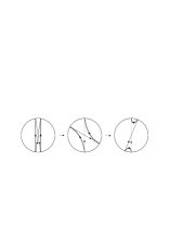
Figure 1: The continuous deformation of the contour $0<\omega<4\pi$ to a point. The deformation is shown in the plane containing the vector $k$ determining the rotation axis. A dashed line denotes the identification of antipodal points of the boundary circle.

If the angle $\omega$ takes values in an interval containing the interval $2\pi$ an odd number of times, then the topological charge equals 1.

Degenerate solutions II.

$$\omega=0,~{}~{}\theta(x),\varphi(x)\in{\cal C}^{2}(L).$$ (37)

Rotation is absent in this series of solutions because the rotation angle equals zero.

Degenerate solutions III.

$$\begin{split}{\sf\,cos\,}\frac{\omega}{2}&=\sqrt{1-\frac{c^{2}}{4b^{2}}}{\sf\,sin\,}[b(x+x_{0})],~{}~{}~{}~{}2|b|\geq|c|\neq 0,\\ \theta&=\frac{\pi}{2},\\ {\sf\,tg\,}(\varphi+\varphi_{0})&=\frac{c}{2b}{\sf\,tg\,}[b(x+x_{0})].\end{split}$$

The polar angle $\varphi$ is a monotonic function of $x$ for these solutions, i.e., the rotation axis $k^{i}$ rotates in the $XY$ plane. Here, the rotation angle changes within the finite interval

$$2{\sf\,arccos\,}\sqrt{1-\frac{c^{2}}{4b^{2}}}<\omega<2\pi-2{\sf\,arccos\,}\sqrt{1-\frac{c^{2}}{4b^{2}}}.$$

It can be easily verified that these solutions are homotopic to zero.

Degenerate solutions IV.

$$\begin{split}{\sf\,cos\,}\frac{\omega}{2}&=\sqrt{1-\frac{c^{2}}{4b^{2}}}{\sf\,sin\,}[b(x+x_{0})],~{}~{}~{}~{}2|b|\geq|c|\neq 0,\\ {\sf\,tg\,}(\theta+\theta_{0})&=\frac{c}{2b}{\sf\,tg\,}[b(x+x_{0})],\\ \varphi&=\varphi_{0}.\end{split}$$

These solutions essentially coincide with degenerate solutions III, but the rotation axis rotates in the $\varphi=\varphi_{0}$ plane.

A general situation. To solve system of equations (34)–(36) in a general situation, we introduce the new coordinate

$$u=\int^{x}\frac{dy}{1-{\sf\,cos\,}\omega(y)}.$$ (38)

The coordinate $u$ increases with increasing of $x$ because $dx/du=1-{\sf\,cos\,}\omega\geq 0$. Equations (35) and (36) then coincide exactly with Eqs. (22) and (23) for $\Theta$ and $\Phi$, in which differentiation with respect to $x$ must be replaced with the differentiation with respect to $u$. Because these equations were analyzed in the previous section, it suffices to solve only Eq. (34). In a general situation, it becomes

$$\omega^{\prime\prime}=c^{2}\frac{{\sf\,sin\,}\omega}{(1-{\sf\,cos\,}\omega)^{2}},~{}~{}~{}~{}c\neq 0.$$ (39)

A general solution of this equation is

$${\sf\,cos\,}\frac{\omega}{2}=\sqrt{1-\frac{c^{2}}{4b^{2}}}{\sf\,sin\,}[b(x+x_{0})],~{}~{}~{}~{}2|b|\geq|c|.$$ (40)

Integral (38) can then be easily taken,

$${\sf\,tg\,}(cu)=\frac{c}{2b}{\sf\,tg\,}[b(x+x_{0})],$$ (41)

where an integration constant is inessential. A solution of Eqs. (35) and (36) has the form

$$\begin{split}{\sf\,cos\,}\theta&=\sqrt{1-\frac{a^{2}}{c^{2}}}{\sf\,sin\,}[c(u+u_{0})],~{}~{}~{}~{}|c|>|a|\neq 0,\\ {\sf\,tg\,}(\varphi+\varphi_{0})&=\frac{a}{c}{\sf\,tg\,}[c(u+u_{0})].\end{split}$$

An elementary geometrical analysis shows that solutions in a general situation essentially coincide with degenerate solutions III and IV, but the rotation axis rotates in the plane tilted at the angle ${\sf\,arccos\,}(a/c)$ to the $XY$ plane.

For static solutions, the energy of the two-dimensional ${\mathbb{S}}{\mathbb{O}}(3)$ model is

$$E=\int_{0}^{L}dx\left(\frac{1}{2}\omega^{\prime 2}+(1-{\sf\,cos\,}\omega)\left(\theta^{\prime 2}+{\sf\,sin\,}^{2}\theta\varphi^{\prime 2}\right)\right).$$

Directly substituting the solutions in this integral, we obtain the values

$$E=\left\{\begin{aligned} 0,&~{}~{}~{}~{}\text{degenerate solutions II},\\ \frac{1}{2}b^{2}L,&~{}~{}~{}~{}\text{degenerate solutions I},\\ 2b^{2}L,&~{}~{}~{}~{}\text{all other solutions}.\end{aligned}\right.$$

The energy is finite for finite $L$. Degenerate solutions II correspond to the absolute minimum because the energy is positive definite.

8 Projective ${\mathbb{R}}{\mathbb{P}}^{d}$ models

The Lagrangian for the Skyrme model written in form (11) can be naturally generalized to the case where the target space is the real projective space ${\mathbb{R}}{\mathbb{P}}^{d}$ of arbitrary dimension. Let $k^{i}$, $i=1,\dotsc,d$, be a unit vector $(k^{2}=1)$ in the Euclidean space ${\mathbb{R}}^{d}$. We consider a vector $k^{i}(x)$ and scalar $\omega(x)$ fields on an arbitrary Minkowski space, $x\in{\mathbb{R}}^{1,n-1}$. Obviously, the Lagrangian

$$\begin{split}L=A\partial_{\alpha}\omega^{2}+B(\partial_{\alpha}k\partial_{\alpha}k)+C(\partial_{\alpha}k\partial_{\alpha}k)\partial_{\beta}\omega^{2}+D&(\partial_{\alpha}k\partial_{\beta}k)\partial_{\alpha}\omega\partial_{\beta}\omega\\ +E(\partial_{\alpha}k\partial_{\alpha}k)^{2}+F&(\partial_{\alpha}k\partial_{\beta}k)^{2}+G(\partial_{\alpha}\omega^{2})^{2}+U,\end{split}$$ (42)

where $A(\omega),B(\omega),C(\omega),D(\omega),E(\omega),F(\omega),G(\omega)$, and $U(\omega)$ are arbitrary periodic (with period $2\pi$) functions of $\omega$, is invariant under transformations (12). In the Lagrangian, we can introduce an isotopic vector field $\omega^{i}=\omega k^{i}$ all of whose components are independent, as in the Skyrme model. Because of equivalence relation (3), an isotopic vector field $\omega^{i}$ can be considered to take values inside a ball of radius $\pi$ with identified antipodal points on the boundary sphere. This means that the field $\omega^{i}$ takes values in an arbitrary projective space ${\mathbb{R}}{\mathbb{P}}^{d}$.

This is the most general invariant Lagrangian depending only on first derivatives of fields raised to a power not exceeding four. It is invariant under the Poicaré group ${\mathbb{I}}{\mathbb{O}}(1,n-1)$ acting in the Minkowski space ${\mathbb{R}}^{1,n-1}$, the rotation group ${\mathbb{O}}(d)$ acting in the target space ${\mathbb{R}}^{d}$, and translations (12). The rotation group ${\mathbb{O}}(d)$ can be extended to the group ${\mathbb{O}}(d+1)$ (maximal symmetry group of the projective space ${\mathbb{R}}{\mathbb{P}}^{d}$), but additional transformations act nonlinearly on fields the $\omega^{i}$.

9 Conclusion

We have considered the Skyrme model as a ${\mathbb{S}}{\mathbb{O}}(3)$ model where the target space is the group manifold itself, and we used the explicit parameterization of the group ${\mathbb{S}}{\mathbb{O}}(3)$ in terms of elements of its algebra. Because the fundamental group of the rotation group is nontrivial, $\pi({\mathbb{S}}{\mathbb{O}}(3))={\mathbb{Z}}_{2}$, the model admits the existence of topologically nontrivial one-dimensional solutions. The corresponding static solutions of the two-dimensional Skyrme model are found and analyzed (degenerate solutions I in Sec. 7).

The form of the action for the ${\mathbb{S}}{\mathbb{U}}(2)$ and ${\mathbb{S}}{\mathbb{O}}(3)$ Skyrme models is the same because their Lie algebras coincide. The difference is in the equivalence relations in the parameter space. Hence, to construct models in mathematical physics, we must not only specify the action but also determine which manifold is the target space. This is important because it may lead to topologically nontrivial solutions of the Euler–Lagrange equations. For example, when considering spinors on a three-dimensional Riemannian manifold, the ${\mathbb{S}}{\mathbb{O}}(3)$ connection enters the covariant derivative, although the spinors transform under the representation of unitary group ${\mathbb{S}}{\mathbb{U}}(2)$. This is because the group ${\mathbb{S}}{\mathbb{O}}(3)$, not the group ${\mathbb{S}}{\mathbb{U}}(2)$, acts on an orthogonal vielbein in the tangent space to a Riemannian manifold.

The ${\mathbb{S}}{\mathbb{O}}(3)$ model can be naturally generalized to the projective space ${\mathbb{R}}{\mathbb{P}}^{d}$ of arbitrary dimension because the group ${\mathbb{S}}{\mathbb{O}}(3)$, as a manifold, is diffeomorphic to the three-dimensional real projective space ${\mathbb{R}}{\mathbb{P}}^{3}$. This allows defining a new class of projective models depending on eight arbitrary periodic functions of one argument. Topologically nontrivial one-dimensional solutions may exist in all these models because $\pi({\mathbb{R}}{\mathbb{P}}^{d})={\mathbb{Z}}_{2}$ for $d\geq 2$.

The ${\mathbb{S}}{\mathbb{O}}(3)$ model can be used in the geometric theory of defects [16, 17]. The Riemann–Cartan geometry can be used to describe the static distribution of dislocations and disclinations in elastic media. The corresponding action is invariant under general coordinate transformations and local ${\mathbb{S}}{\mathbb{O}}(3)$ rotations. The equations of elasticity theory were recently used to fix the coordinate system [18]. This allowed including the classical elasticity theory in the geometric approach as a limiting case where defects are absent. The ${\mathbb{S}}{\mathbb{O}}(3)$ model discussed in the present paper can be used to fix local ${\mathbb{S}}{\mathbb{O}}(3)$ rotations because it is not invariant under these rotations. In this case, the geometric theory of defects yields the ${\mathbb{S}}{\mathbb{O}}(3)$ model in the absence of disclinations. For example, the Lorenz gauge for the ${\mathbb{S}}{\mathbb{O}}(3)$ connection results in the equations of the principal chiral field for the group ${\mathbb{S}}{\mathbb{O}}(3)$ in the absence of disclinations. In the limit of no dislocations and disclinations, the geometric defect theory can therefore be reduced to the equations of the elasticity theory for the shift vector and to the equations of the principal chiral field for the spin structure.

The author is very grateful to I. V. Volovich, R. Dandoloff, E. A. Ivanov, A. I. Pashnev, for the useful discussion and comments and to the Erwin Schrödinger Institute (Vienna) for the hospitality. This work was supported in part by the Russian Foundation for Basic Research (grants 96-15-96131 and 02-01-01084).

References

• [1] T.Β H.Β R. Skyrme. Nonlinear field theory. Proc.Β Roy.Β Soc. London, A260:127–138, 1961.
• [2] V.Β E. Zakharov, S.Β V. Manakov, S.Β P. Novikov, and L.Β P. Pitaevskii. The Inverse Scattering Method. Nauka, Moscow, 1980. [in Russian]; English transl.: S.Β P.Β Novikov, S.Β V.Β Manakov, L.Β P.Β Pitaevskii, and V.Β E.Β Zakharov The Inverse Scattering Method Plenum, New York (1984).
• [3] R.Β Rajaraman. Solitons and Instantons in Quantum Field Theory. North–Holland, Amsterdam, 1982.
• [4] L.Β A. Takhtadzhyan and L.Β D. Faddeev. The Hamiltonian Methods in the Theory of Solitons. Nauka, Moscow, 1986. [in Russian]; English transl.: L.Β D.Β Faddeev and L.Β A.Β Takhtajan The Hamiltonian Methods in the Theory of solitons, Berlin, Springer (1987).
• [5] W.Β J. Zakrzewski. Low Dimensional Sigma Models. Adam Hilger, Bristol – Philadelphia, 1989.
• [6] Yu.Β P. Rybakov and V.Β I. Sanyuk. Multidimensional Solitons. Russian Univ. of People’s Friendship Publ., Moscow, 2001. [in Russian].
• [7] A.Β A. Belavin and A.Β M. Plyakov. Metastable states of two-dimensional isotropic ferromagnet. JETP Letters, 22(10):245–247, 1975.
• [8] J.Β P. Elliott and P.Β G. Dawber. Symmetry in Physics, volume 2: Further Applications. The Macmillan Press Ltd, London, 1979.
• [9] B.Β A. Dubrovin, S.Β P. Novikov, and A.Β T. Fomenko. Modern geometry: Methods and Applications. Nauka, Moscow, fourth edition, 1998. [In Russian]; English transl.Β prev.Β ed.: B.Β A.Β Dubrovin, A.Β T.Β Fomenko, and S.Β P.Β Novikov Modern Geometry: Methods and Applications, Part 1, The Geometry of Surfaces, Transformation Groups, and Fields, Springer, New York (1992).
• [10] L.Β D. Faddeev. In search of multidimensional solitons. In Nonlocal. Nonlinear, and Nonrenormalizable Field Theories, pages 207–223, Dubna, 1977. Joint Inst.Β Nucl.Β Res. [in Russian].
• [11] L.Β Faddeev and A.Β J. Niemi. Partially dual variables in ${{\mathbb{S}}{\mathbb{U}}(2)}$ Yang–Mills theory. Phys.Β Rev.Β Lett., 82:1624–1627, 1999.
• [12] L.Β Faddeev and A.Β J. Niemi. Knots and particles. Nature, 387:58–66, 1997.
• [13] R.Β A. Battye and P.Β Sutcliffe. Knots as stable soliton solurions in a three-dimensional classical field theory. Phys.Β Rev.Β Lett., 81:4798–4801, 1998.
• [14] R.Β A. Battye and P.Β Sutcliffe. Solitons, links and knots. Proc.Β Roy.Β Soc.Β London, A455:4305–4331, 1999.
• [15] J.Β Hietarinta and P.Β Salo. Faddeev–hopf knots: dynamics of linked unknots. Phys.Β Lett., B451:60–67, 1999.
• [16] M.Β O. Katanaev and I.Β V. Volovich. Theory of defects in solids and three-dimensional gravity. Ann.Β Phys., 216(1):1–28, 1992.
• [17] M.Β O. Katanaev and I.Β V. Volovich. Scattering on dislocations and cosmic strings in the geometric theory of defects. Ann.Β Phys., 271:203–232, 1999.
• [18] M.Β O. Katanaev. Wedge dislocation in the geometric theory of defects. Theor.Β Math.Β Phys., 135(2):733–744, 2003.