Exact String-like Solutions of the Gauged Nonlinear O(3) Model

Abstract

We show that the least energy conditions in the gauged nonlinear sigma model with Chern-Simons term lead to exact soliton-like solutions which have the same features as domain walls. We will derive and discuss the corresponding solutions, and compute the total energy, charge, and spin of the resulting system.

I Introduction

The O(3) sigma model in (2+1) dimensions is a popular model in theoretical physics and has been studied extensively sch bel . As far as static solutions are concerened, the model is integrable and of Bogomol’nyi type bog . The exact solutions are therefore available via simple analytical expressions. In contrast, similar models in (3+1) dimensions (bar ,pey ,pie ,sky ), are neither integrable nor of Bogomol’nyi type. Nevertheless, the soliton solutions of models in 3+1 dimensions are extensively studied numerically and have found application in particle and nuclear physics wit . Soliton solutions in (2+1) dimensions, modified by the addition of the Hopf term are topologically stable and are classified according to the homotopy $\pi_{2}(S^{2})=Z$. These solutions are scale-invariant. This property leads to some difficulties upon quantization. Moreover, upon interacting with each other, solitons undergo change of size and tend to become singular lee . The soliton solutions of the O(3) sigma model with a suitable choice of potential are presented explicitly in lee2 together with their interaction behavior. These solitons are also called Q-lumps.

There are two natural ways for breaking the scale-invariance: gauging the symmetry, and including a potential term sch . It has been shown that gauging the U(1) subgroup by a Chern-Simons term and including a suitable potential leads to both topological and nontopological solitons which are not scale-invariant gho . The potential discussed in gho has two discrete minima $\phi_{3}=\pm 1$ for which the U(1) symmetry is not spontaneously broken in (2+1) dimensions. This model was further studied by Mukherjee muk , where it was shown that the degeneracy of topological solitons is removed by including a potential with symmetry-breaking minima. Solutions with azimuthal vector potentials (${\bf A}=\hat{\theta}\frac{n}{r}$), have quantized magnetic flux ($\Phi=2\pi n$), spin ($S=-\pi kn^{2}$), and charge ($Q=-2\pi kn$).

In the present paper, we will show that within the framework of the model presented in muk , exact soliton solutions exist which depend on one spatial dimension, resembling domain-wall solutions of the $\phi^{4}$ theory. Because of the non-trivial mapping between the boundaries and the discrete vacua, the solutions are topologically stable. The stability and lack of the scale invariance are also verified using the energy functional of the system.

II Gauged O(3) sigma model

The lagrangian of the model considered here, is the one partially studied in muk , in (2+1) dimensions:

$${\cal L}=\frac{1}{2}D_{\mu}\phi.D^{\mu}\phi+\frac{k}{4}\epsilon^{\mu\nu\lambda}A_{\mu}\partial_{\nu}A_{\lambda}-U(\phi).$$ (1)

Here $\phi=(\phi_{1},\phi_{2},\phi_{3})$ is a triplet of scalar fields, constrained to a $S^{2}$:

$$\phi_{a}\phi_{a}=1,$$ (2)

where

$$\phi_{a}=n_{a}.\phi,$$ (3)

and $n_{a}$ (a=1,2,3) are unit orthogonal vectors in the internal space. We work in the Minkowski spacetime with the metric tensor $g_{\mu\nu}=(1,-1,-1)$. $D_{\mu}\phi$ is the covariant derivative given by sch :

$$D_{\mu}\phi=\partial_{\mu}\phi+A_{\mu}{\bf n}\times\phi,$$ (4)

where ${\bf n}$ is the (constant) unit vector defined by

$${\bf n}=\lim_{|x|\rightarrow\infty}{\bf\phi}(t,{\bf x}).$$ (5)

The U(1) subgroup is gauged by the vector potential $A_{\mu}$ whose dynamics is dictated by the Chern-Simons term. The potential

$$U(\phi)=\frac{1}{2k^{2}}\phi_{3}^{2}(1-\phi_{3}^{2})$$ (6)

gives a self interaction of the field $\phi_{a}$. Note that the minima of the potential reside either on,

$$\phi_{1}=\phi_{2}=0\ \ {\rm and}\ \ \phi_{3}\pm 1,$$ (7)

or

$$\phi_{3}=0\ \ {\rm and}\ \ \phi_{1}^{2}+\phi_{2}^{2}=1.$$ (8)

In 2+1 dimensions, soliton solutions of this system has been studied muk . In such a case, the U(1) symmetry is unbroken in (7), whereas (8) corresponds to the spontaneous breaking of this symmetry.

In 1+1 dimensions, we expect that the disconnected vacua facilitate the existence of solitons. Because of the existence of disconnected vacua, we can have non-trivial mappings between the boundaries of the 1-dimensional space and these disconnected vacua and thus topological stability (Figure 1). In order to obtain these soliton solutions, we start with Schwinger’s energy-momentum tensor shw , which in the static limit becomes:

$$E=\frac{1}{2}\int d^{2}x\left(D_{i}\phi.D_{i}\phi+\frac{k^{2}B^{2}}{1-\phi_{3}^{2}}+\frac{1}{k^{2}}\phi_{3}^{2}(1-\phi_{3}^{2})\right),$$ (9)

where $B=curl(A)$ is the magnetic field. A conserved current can also be constructed:

$$K_{\mu}=\frac{1}{8\pi}\epsilon_{\mu\nu\lambda}\left[\phi.D^{\nu}\phi\times D^{\lambda}\phi-F^{\nu\lambda}\phi_{3}\right].$$ (10)

For static solutions which depend on one space coordinate (say $x$), $K_{o}$ becomes:

$$K_{o}=-\frac{1}{4\pi}\left[A_{2}\phi_{3}\frac{\partial\phi}{\partial x}.\phi+\frac{\partial\phi_{3}}{\partial x}\right]+\frac{1}{4}\phi_{3}\frac{\partial A_{2}}{\partial x},$$ (11)

and the corresponding conserved total charge is:

$$T=\int dxK_{o}.$$ (12)

We also have

$$B=F_{12}=\frac{\partial A_{2}}{\partial x},$$ (13)

with

$$A_{2}=\frac{\phi_{3}}{k},$$ (14)

which leads to

$$B=\frac{1}{k}\frac{d\phi_{3}}{dx}.$$ (15)

Rearranging (9), we can write gho raj :

$$E=\int d^{2}x\left[\frac{1}{2}(D_{i}\phi\pm\epsilon_{ij}\phi\times D_{j}\phi)^{2}+\frac{k^{2}}{1-\phi_{3}^{2}}\left(F_{12}\pm\frac{1}{k^{2}}\phi_{3}(1-\phi_{3}^{2})\right)^{2}\right]\pm 4\pi T.$$ (16)

This leads to the Bogomol’nyi conditions:

$$D_{i}\phi\pm\epsilon_{ij}\phi\times D_{j}\phi=0,$$ (17)

and

$$F_{12}\pm\frac{1}{k^{2}}\phi_{3}(1-\phi_{3}^{2})=0,$$ (18)

which minimize the energy functional in a particular topological sector.

Figure 1: String-like solutions correspond to mappings between the boundaries of $x$ and the disconnected vacua of the $\phi$-fields.

III Exact Domain wall solutions

In this section, we obtain analytical domain-wall-like solutions in the case where the fields depend on only one of the space coordinates (say $x$). The $\phi$-fields, which are constrained on a $S^{2}$, are assumed to vary on a longitude. Because of the U(1) subgroup, this longitude is arbitrarily rotated to $\phi_{2}=0$, in order to simplify the solutions. Let us expand the Bogomol’nyi equations (17) and (18) as:

$$\frac{\partial\phi_{1}}{\partial x}\mp\phi_{3}\phi_{1}A_{2}=0,$$ (19)

$$\frac{\partial\phi_{3}}{\partial x}\pm A_{2}\mp\phi_{3}^{2}A_{2}=0,$$ (20)

$$\pm A_{1}\phi_{3}\phi_{1}=0,$$ (21)

$$\phi_{1}A_{2}\pm(\phi_{1}\frac{\partial\phi_{3}}{\partial x}-\phi_{3}\frac{\partial\phi_{1}}{\partial x})=0,$$ (22)

and

$$\mp A_{1}\pm A_{1}\phi_{3}^{2}=0.$$ (23)

It can be easily shown that the above equations, together with appropriate boundary conditions, lead to:

$$\frac{\partial\phi_{3}}{\partial x}-A_{2}(1-\phi_{3}^{2})=0,$$ (24)

and

$$A_{1}(1-\phi_{3}^{2})^{1/2}=0,$$ (25)

which implies

$$A_{1}=0.$$ (26)

Note that $\phi_{3}^{2}\neq 1\ \ \forall x$ for the desired solutions. We also have

$$\frac{\partial A_{2}}{\partial x}\pm\frac{1}{k^{2}}\phi_{3}(1-\phi_{3}^{2})=0.$$ (27)

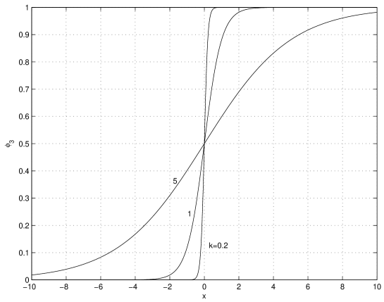
Equations (24) and (27) are readily solved to obtain

$$\phi_{3}=\pm\frac{1}{(1+e^{-\frac{2x}{k}})^{1/2}},$$ (28)

$$A_{1}=0.$$ (29)

and

$$A_{2}=\frac{\phi_{3}}{k},$$ (30)

From these, the $B$ field is also calculated:

$$B=F_{12}=\frac{\partial A_{2}}{\partial x},$$ (31)

or

$$B=\pm\frac{1}{k^{2}}\frac{\partial\phi_{3}}{\partial x}=\frac{e^{-\frac{2x}{k}}}{k(1+e^{-\frac{2x}{k}})^{3/2}}.$$ (32)

$\phi_{3}(x)=kA_{2}(x)$ is plotted in Figure 2, and $B(x)$ is shown in Figure 3.

Figure 2: Variation of the $\phi_{3}$ field as a function of the $x$-coordinate for $k=0.2,1.0,\ {\rm and}\ 5$.

Figure 3: Variation of the magnetic field $B$ as a function of the $x$-coordinate for $k=0.2,1.0,\ {\rm and}\ 5$.

IV Conserved Quantities and Stability

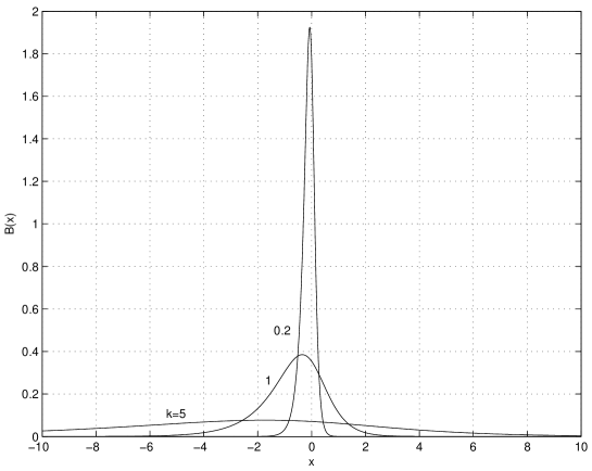
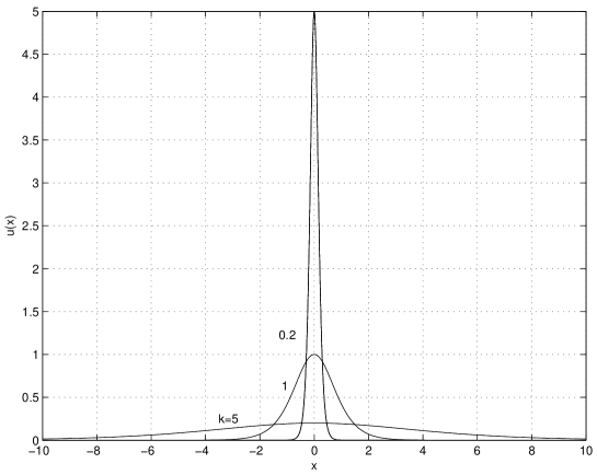
Using (9), the energy density can be easily calculated

$$u=\frac{4}{k^{2}}\frac{e^{-2x/k}+e^{-4x/k}}{(1+e^{-2x/k})^{3}},$$ (33)

which is plotted in Figure (4). It is seen that the magnetic field and energy are concentrated in a thin region around $x=0$, quite similar to the domain wall solutions of the $\phi^{4}$ theory in (3+1) dimensions. Here, the solution corresponds to a string on the $xy$-plane which extends along the $y$-axis. Integrating the energy density over $x$, the total energy per unit length of the string is obtained:

$$E=\int_{-\infty}^{+\infty}u(x)dx=\frac{2}{k^{2}}.$$ (34)

In order to check for the stability of the solution, we apply the scale transformation

$$x\rightarrow\alpha x$$ (35)

which leads to

$$E\rightarrow E(\alpha)=\frac{1}{\alpha}f+\alpha g,$$ (36)

where $f$ and $g$ are positive quantities independent of $\alpha$. The energy is found to be a minimum at $\alpha=1$, signalling the stability.

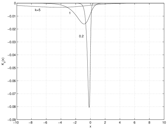
Let us calculate the topological charge density (the zero component of topological current). From (11), we obtain

$$K_{o}=\frac{1}{4\pi k^{2}}\frac{e^{-2x/k}}{(1+e^{-2x/k})^{3/2}}\left[\frac{1}{(1+e^{-2x/k})^{1/2}}-1\right],$$ (37)

which is shown in Figure (5). The total topological charge is subsequently obtained:

$$T=\int_{-\infty}^{+\infty}K_{o}(x)dx=-\frac{0.0398}{k^{2}}\ \ \ {\rm(numerical)}.$$ (38)

The values of $E$ and $T$ are seen to satisfy the well known inequality $E\geq 8\pi T$.

The spin of the solution ban1a ban2 is easily shown to vanish:

$$S_{i}=-\frac{k}{2}\oint_{boundary}(x_{i}A^{2}-A_{i}x_{j}A^{j})n^{i}dl=0.$$ (39)

Figure 4: Variation of the energy density $u(x)$ as a function of the $x$-coordinate for $k=0.2,\ 1.0,\ {\rm and}\ 5.0$.

Figure 5: Variation of the charge density $K_{o}$ as a function of the $x$-coordinate for $k=0.2,\ 1.0,\ {\rm and}\ 5.0$.

V Conclusion

In a field theory possessing the vacuum manifold ${\cal M}$, formulated in a D-dimensional space plus 1 time dimension, the localized static solutions constitute a mapping $\pi:\partial M\rightarrow\cal{M}$, where $\partial M$ is the boundary of the D-dimensional space. If the homotopy group of this mapping is nontrivial, then topological, soliton-like solutions are expected ria . We showed that the nonlinear O(3) sigma model with a Chern-Simons term and a suitable potential is such a model. We obtained examples of these solutions which satisfy the Bogomol’nyi’s conditions. On the $xy$-plane, solutions correspond to a string along the $y$-axis, with energy density, charge density, and magnetic field confined to a thin band near to $x=0$. The width of this band (string) depends on the value of the parameter $k$. We also showed that the solutions are not scale invariant under $x\rightarrow\alpha x$. Rather, the energy is minimum for $k=1$, indicating the stability of the solutions.