UNITU–THEP–25/2002 FAU-TP3-02/27
http://xxx.lanl.gov/abs/hep-th/0304134
 
 
On the infrared behaviour of Gluons and Ghosts in
Ghost-Antighost symmetric gauges

Abstract

To investigate the possibility of a ghost-antighost condensate the coupled Dyson–Schwinger equations for the gluon and ghost propagators in Yang–Mills theories are derived in general covariant gauges, including ghost-antighost symmetric gauges. The infrared behaviour of these two-point functions is studied in a bare-vertex truncation scheme which has proven to be successful in Landau gauge. In all linear covariant gauges the same infrared behaviour as in Landau gauge is found: The gluon propagator is infrared suppressed whereas the ghost propagator is infrared enhanced. This infrared singular behaviour provides indication against a ghost-antighost condensate. In the ghost-antighost symmetric gauges we find that the infrared behaviour of the gluon and ghost propagators cannot be determined when replacing all dressed vertices by bare ones. The question of a BRST invariant dimension two condensate remains to be further studied.

Keywords: Confinement; Non–perturbative QCD; Running coupling constant;
Gluon propagator; Dyson–Schwinger equations; Infrared behavior.

PACS: 12.38.Aw 14.70.Dj 12.38.Lg 11.15.Tk 02.30.Rz

I Introduction

A large body of experimental data supports the general believe that Quantum Chromodynamics (QCD) is the correct theory of strong interactions. Nevertheless we are left with the task of understanding the physics of hadrons, and hereby in particular the mechanisms of confinement and spontaneous breaking of chiral symmetry. Gaining such an insight requires reliable non-perturbative treatments of QCD. Hereby Monte Carlo lattice calculations provide a rigorous non-perturbative approach to QCD. They have the advantage of fully respecting gauge invariance independently of the size of the lattice used. On the other hand, the extraction of the continuum values of physical observables from the lattice data requires a careful study of the scaling regime. The observed scaling behaviour, however, will be in general contaminated by finite size effects. With respect to studies of the confinement mechanisms this is problematic: As infrared singularities are expected to occur in QCD there is definite need for a continuum-based non-perturbative approach.

To this end we note that the Schwinger–Dyson equations of QCD can address directly the infrared region. They provide genuine non-perturbative information and are at the same time fully formulated in the continuum theory. Such an approach is, however, less rigorous than lattice calculations in the sense that truncations of the tower of coupled equations are necessary in practical calculations. Justifications for such truncations can be given on the basis of general principles like e.g. a restriction to the first Gribov region, see ref. Zwanziger:2003cf and references therein. Nevertheless, the validity of the employed truncation is finally judged by comparing its results with either the results of Monte Carlo calculations or experiments. The latter is easily possible as the Schwinger–Dyson approach has been successfully applied to the description of hadron phenomenology, see e.g. the recent reviews refs. Roberts:2000aa ; Alkofer:2001wg and references therein. Furthermore, despite recent progress by improved lattice algorithms, and despite the increasing computer time available for lattice calculations, including dynamical fermions is exceedingly cumbersome and finite baryon densities are hardly accessibly in realistic SU(3) lattice simulations. On the other hand, dynamical fermions and finite baryon densities can be relatively easily treated in the Schwinger–Dyson approach to QCD.

In recent years the fundamental Schwinger–Dyson equations of SU(N) Yang-Mills theories have been solved explicitly in certain approximations yielding gluon and ghost propagators Alkofer:2001wg ; vonSmekal:1997is ; Atkinson:1998tu ; Zwanziger:2001kw ; Lerche:2002ep ; Fischer:2002hn . In these calculations, carried out in Landau gauge, vertex functions constructed from appropriate Slavnov-Taylor identities as well as bare vertices have been employed. The results proved to be qualitatively similar among each other and agree well with recent lattice calculations Bonnet:2000kw ; Bonnet:2001uh ; Langfeld:2001cz ; Suman:1995zg ; Cucchieri:1997dx for both, the gluon and ghost propagator. The common, though gauge dependent, result of both approaches is an infrared suppressed gluon propagator and an infrared enhanced ghost propagator. Furthermore, the inclusion of dynamical quarks does not alter the infrared behaviour of gluon and ghost propagators and leads to only slight modifications for non-vanishing momenta for the number of light flavours $N_{f}\leq 3$ Fischer:2003rp . These results especially imply that the ghosts take the role of the long range correlations in the theory. Such a behaviour is in accordance with the Gribov–Zwanziger horizon condition, see e.g. ref. Zwanziger:2001kw and references therein, and the Kugo–Ojima confinement criterion, which in Landau gauge includes the statement that the ghost propagator should be more singular than a simple pole Kugo:1979gm .

The central assumption in the Kugo–Ojima confinement scenario is the invariance of the measure of the functional integral under BRS transformations and the existence of a nilpotent BRS-operator Nakanishi . The most general Lorentz invariant and globally gauge invariant Lagrangean of dimension four that can be constructed under this assumption has been derived in ref. Baulieu:1982sb . In addition to the structure appearing in ordinary linear covariant gauges, the Lagrangean contains a second gauge parameter which controls the symmetry of the Lagrangean under ghost-antighost interchange. Furthermore a four ghost interaction term is present. We will use this Lagrangean as the starting point of our investigation.

Our main interest in this paper will be to explore the situation in these general covariant gauges. Away from the Landau gauge limit the connection between the Kugo–Ojima confinement criterion and the infrared behaviour of the ghost dressing function is far from obvious. In particular, the question might arise whether it is possible that the infrared dominant role of the ghost dressing function, seen in the Landau gauge, is assumed by other degrees of freedom like the longitudinal gluons in other covariant gauges. As a matter of fact, infrared dominance of longitudinal gluons is seen if stochastic quantization is used instead of the Faddeev–Popov quantization Zwanziger:2002ia . Furthermore, calculations based on many-body techniques provide evidence that in Coulomb gauge (employing the usual Faddeev–Popov quantization) the ghosts and the Coulomb gluons are both infrared enhanced Szczepaniak:2001rg . This latter picture for Coulomb gauge QCD obtains (at least partial) support from lattice Cucchieri:2001zb and renormalization group calculations Cucchieri:2000hv . Care has, however, to be taken as the Coulomb gauge limit is highly non-trivial, see ref. e.g. Baulieu:1998kx . On the other hand, the benefit of Coulomb gauge is obvious. The time-time component of the gluon propagator and the heavy quark potential fulfill a strictly valid inequality Cucchieri:2000hv ; Zwanziger:2002sh with the Coulomb string tension being several times larger than the asymptotic one Greensite:2003xf . Even more important, quark confinement directly results from infrared enhanced Coulomb gluons, see e.g. refs. Szczepaniak:1996tk ; Alkofer:tc and references therein. Instead of exploring the correlation functions in non-covariant gauges we will in this paper study Green’s functions in covariant albeit non-linear gauges.

Ghost-antighost symmetric gauges are of special interest when investigating the possibility of a BRST invariant condensate of dimension two in QCD. Such condensates occur in the operator product expansion of the gluon propagator Lavelle:eg ; Boucaud:2001st ; Kondo:2001nq , bear some relation to the Gribov problem Stodolsky:2002st , may result in gluon mass generation Dudal:2003gu and may be important for confinement in general Schaden:1999ew ; Gubarev:2000eu . Hereby it has been clarified recently that these condensates are highly non-local Dan ; Pierre and that they are only BRST invariant after eliminating the Nakanishi–Lautrup field via its equation of motion Gripaios:2003xq . This kind of restricted BRST invariance has been called ‘on-shell BRST invariance’ and can be related to a residual gauge symmetry after gauge fixing.

The solutions of the gluon and ghost Dyson–Schwinger equations in Landau gauge provide a somewhat different picture: Whereas the operator product expansion of the gluon propagator requires such a dimension two condensate its interpretation with respect to a gluon mass is made impossible by the gluon propagator’s infrared behaviour $D(p^{2}=0)=0$ instead of $D(p^{2}=0)=1/m^{2}$. Also the highly infrared singular ghost propagator excludes a ghost mass and/or a ghost-antighost condensate. Therefore the question arises whether in general ghost-antighost symmetric gauges the infrared behaviour of the propagators can be interpreted in terms of gluon and ghost “masses”.

This paper is organized as follows: In sect. 2 we summarize some properties of the general Lagrangean given in ref. Baulieu:1982sb and outline the derivation of the coupled set of Dyson–Schwinger equations (DSEs) for the ghost and gluon propagators. As the Lagrangean contains a four–ghost interaction a rich structure in the ghost DSE emerges which closely resembles the one already present in the gluon equation of ordinary linear covariant gauges. In sect. 3 we employ a truncation scheme that has proven to be successful in Landau gauge and study in particular the infrared behaviour of the ghost and gluon dressing functions for general values of the two gauge parameters. Furthermore, we show that in the ghost-antighost symmetric gauges the contributions of the genuine two-loop terms (generalized squint and sunset diagram) in the gluon and the ghost DSEs must be properly taken into account in the infrared. In the linear covariant gauges no such terms are present in the ghost DSE, and selfconsistent results can be obtained assuming the two-loop terms in the gluon equation to be subleading in the infrared . In general ghost-antighost symmetric gauges, on the other hand, the bare-vertex truncation is insufficient to clarify the infrared behaviour of the gluon and ghost propagators. In sect. 4 we will provide numerical solutions for the DSEs in the Landau gauge limit of the ghost–antighost symmetric case of the Lagrangean and recover the solutions found in Fischer:2002hn from a different direction in two dimensional gauge parameter space. In the last section we give our conclusions. Technical details are deferred into four appendices.

II The Dyson–Schwinger equation for the ghost propagator

II.1 Renormalized double BRS symmetry

The most general Lagrangean of dimension four that is Lorentz invariant, globally gauge invariant, invariant under BRST- and anti-BRST-transformations, hermitean and omitting topological terms, is Baulieu:1982sb :

$$\cal{L} = \frac{1}{4}F_{\mu\nu}^{2}+\frac{\left(\partial_{\mu}A_{\mu}\right)^{2}}{2\lambda}+\frac{\alpha}{2}\left(1-\frac{\alpha}{2}\right)\frac{\lambda}{2}(\bar{c}\times c)^{2}-i\frac{\alpha}{2}D_{\mu}\bar{c}\partial_{\mu}c-i\left(1-\frac{\alpha}{2}\right)\partial_{\mu}\bar{c}D_{\mu}c.$$ (1)

The field strength tensor and the covariant derivative are defined as

$$F_{\mu\nu}^{a} = \partial_{\mu}A_{\nu}^{a}-\partial_{\nu}A_{\mu}^{a}-gf^{abc}A_{\mu}^{b}A_{\nu}^{c}$$

$$D_{\mu}^{ab} = \partial_{\mu}\delta^{ab}+gf^{abc}A_{\mu}^{c},$$ (2)

and the abbreviation $(\bar{c}\times c)^{a}=gf^{abc}\>\bar{c}^{b}c^{c}$ is used. Note that both ghost and antighost fields, $\bar{c}$ and $c$, resp., are chosen to be hermitean, $c^{\dagger}=c$ and $\bar{c}^{\dagger}=\bar{c}$ . This is necessary to maintain the hermiticity of the Lagrangian for all values of the gauge parameters $\lambda$ and $\alpha$, see e.g. Nakanishi and references therein. Furthermore we work in Euclidean space-time.

From the two gauge parameters of the Lagrangian the first one, $\lambda$, is the usual parameter of linear covariant gauges, whereas the second one, $\alpha$, controls the symmetry properties of the ghost content. For the cases $\alpha=0$ and $\alpha=2$ one recovers the usual Faddeev–Popov Lagrangian and its mirror image, respectively, where the role of ghost and antighost have been interchanged. For the value $\alpha=1$ the Lagrangian is completely symmetric in the ghost and antighost fields.

In ref. Baulieu:1982sb it has been shown that the S-matrix of the theory is invariant under variation of the gauge parameters $\lambda$ and $\alpha$. Therefore gauge invariance of physical observables is ensured. One-loop calculations confirm in particular the independence of the first nontrivial coefficient of the $\beta$ function from the gauge parameters.

Furthermore, the existence of a renormalized BRS-algebra has been proven Baulieu:1982sb , thus the theory given by (1) is multiplicatively renormalizable. From one-loop calculations one finds, that the Faddeev-Popov values of the gauge parameters, $\alpha=0$ and $\alpha=2$, are fixed points under the renormalization procedure. The same is true for the ghost-antighost symmetric case $\alpha=1$. The case of Landau gauge, $\lambda=0$, corresponds to a fixed point as well, because the constraint $\partial_{\mu}A^{\mu}=0$ is not affected by a rescaling of the gluon field.

To be specific the renormalized BRS ($s_{r}$) and anti-BRS ($\bar{s}_{r}$) transformations are given by

$$\begin{array}[]{l@{\hskip 20mm}l}s_{r}A=-\widetilde{Z}_{3}D_{r}c\;,\hfil\hskip 56.9055pt&\bar{s}_{r}A=-\widetilde{Z}_{3}D_{r}\bar{c}\;,\\ \hfil\hskip 56.9055pt&\\ \displaystyle s_{r}c=-\widetilde{Z}_{1}\frac{1}{2}\,(c\times c)\;,\hfil\hskip 56.9055pt&\displaystyle\bar{s}_{r}\bar{c}=-\widetilde{Z}_{1}\frac{1}{2}\,(\bar{c}\times\bar{c})\;,\\ \hfil\hskip 56.9055pt&\\ \displaystyle s_{r}\bar{c}=B-\frac{\alpha}{2}\widetilde{Z}_{1}\,(\bar{c}\times c)\;,\hfil\hskip 56.9055pt&\displaystyle\bar{s}_{r}c=-B-(1-\frac{\alpha}{2})\widetilde{Z}_{1}\,(\bar{c}\times c)\;,\\ \hfil\hskip 56.9055pt&\\ \displaystyle s_{r}B=-\frac{\alpha}{2}\widetilde{Z}_{1}\,(c\times B)\hfil\hskip 56.9055pt&\displaystyle\bar{s}_{r}B=-(1-\frac{\alpha}{2})\widetilde{Z}_{1}\,(\bar{c}\times B)\\ \displaystyle\qquad-\frac{\alpha}{2}(1-\frac{\alpha}{2})\frac{1}{2}{\widetilde{Z}}_{1}^{2}\,\Big{(}(c\times c)\times\bar{c}\Big{)}\;,\hfil\hskip 56.9055pt&\displaystyle\qquad+\frac{\alpha}{2}(1-\frac{\alpha}{2})\frac{1}{2}{\widetilde{Z}}_{1}^{2}\,\Big{(}(\bar{c}\times\bar{c})\times c\Big{)}\;.\end{array}$$ (3)

Here $D_{r}=\partial-Z_{3}^{1/2}Z_{g}(A\times\phantom{A})$ is the covariant derivative in the adjoint representation, with color and Lorentz indices suppressed. Note that the Nakanishi–Lautrup auxiliary field $B$ can be eliminated from the BRS-transformations by using its equation of motion. The corresponding BRS-transformations are called ‘on-shell’. Note furthermore that the application of the BRS-operator $s_{r}$ ($\bar{s}_{r}$) on a field increases (decreases) the ghost number by $+1$ ($-1$), thus we can assign the value $N_{FP}=+1$ ($N_{FP}=-1$) to the (anti-)BRS-operator itself. The BRS-operator and the anti-BRS-operator are nilpotent and related by $s_{r}\bar{s}_{r}+\bar{s}_{r}s_{r}=0$. These properties are, however, lost when considering ‘on-shell’ BRS-transformations.

The Maurer-Cartan conditions, in addition to the forms of $s_{r}c$ and $\bar{s}_{r}\bar{c}$, for ghosts $c$ and anti-ghosts $\bar{c}$ in a ghost anti-ghost symmetric formulation thereby require Baulieu:1982sb

$$s_{r}\bar{c}+\bar{s}_{r}c+\widetilde{Z}_{1}\,(\bar{c}\times c)=0\;.$$ (4)

The correspondence between the bare Lagrangean and its renormalized version including counterterms is given by the following rescaling transformations

$$A_{\mu}^{a} \rightarrow \sqrt{Z_{3}}A_{\mu}^{a},\>\>\>\>\>\>\bar{c}^{a}c^{b}\rightarrow\tilde{Z}_{3}\bar{c}^{a}c^{b},\>\>\>\>\>\>B^{a}\rightarrow B^{a}/\sqrt{Z_{3}}$$

$$g \rightarrow Z_{g}g,\>\>\>\>\>\>\>\>\>\>\>\>\>\alpha\rightarrow Z_{\alpha}\alpha,\>\>\>\>\>\>\>\>\>\>\>\>\>\>\lambda\rightarrow Z_{\lambda}\lambda,$$ (5)

where five independent renormalization constants $Z_{3},\tilde{Z}_{3},Z_{g},Z_{\alpha}$ and $Z_{\lambda}$ have been introduced. Furthermore four additional renormalization constants are related to these via Slavnov–Taylor identities,

$$Z_{1}=Z_{g}Z_{3}^{3/2},\>\>\>\>\>\>\tilde{Z}_{1}=Z_{g}\tilde{Z}_{3}Z_{3}^{1/2},\>\>\>\>\>\>Z_{4}=Z_{g}^{2}Z_{3}^{2},\>\>\>\>\>\>\tilde{Z}_{4}=Z_{g}^{2}\tilde{Z}_{3}^{2}.$$ (6)

Note, however, that contrary to standard Faddeev–Popov gauges $Z_{\lambda}\not=Z_{3}$, e.g., at one-loop (MS scheme), one has

$$Z_{\lambda}=Z_{3}-\frac{g^{2}}{16\pi^{2}}\frac{1}{\epsilon}N_{c}\,\frac{\alpha}{2}(1-\frac{\alpha}{2})\;\lambda\;.$$ (7)

The gauge fixing part of the Lagrangean (1) can be written in the following three equivalent ways,

$$\mathcal{L}_{\mathcal{GF}} = \frac{i}{2}\frac{1}{Z_{3}\widetilde{Z}_{3}}\,s_{r}\bar{s}_{r}\left(Z_{3}\,AA+iZ_{\lambda}\widetilde{Z}_{3}\,\alpha\,\lambda c\bar{c}\right)\,+\,\frac{Z_{\lambda}}{Z_{3}}(1-\alpha)\frac{\lambda}{2}\,s_{r}(\bar{c}\,s_{r}\bar{c})$$ (8)

$$= is_{r}\left(\bar{c}\big{(}\partial A-i\frac{Z_{\lambda}}{Z_{3}}\frac{\lambda}{2}B\big{)}\right)$$

$$= iB\partial A+\frac{Z_{\lambda}}{Z_{3}}\frac{\lambda}{2}B^{2}+\frac{Z_{\lambda}}{Z_{3}}{\widetilde{Z}}_{1}^{2}\,\frac{\alpha}{2}(1-\frac{\alpha}{2})\,\frac{\lambda}{2}(\bar{c}\times c)^{2}+i\widetilde{Z}_{3}\big{(}(1-\frac{\alpha}{2})\,\bar{c}\,\partial D_{r}\,c\,+\,\frac{\alpha}{2}\,\bar{c}\,D_{r}\partial\,c\big{)}\;.$$

This is verified by direct calculation via the transformations defined in Eqs. (3). In the form of Eq. (LABEL:Lgf3) the gauge fixing Lagrangean shows that the renormalization constants introduced in (3) correspond to the replacements of bare by renormalized quantities as given above.

We may rewrite the gauge fixing Lagrangean of Eq. (LABEL:Lgf3) once more,

$$\mathcal{L}_{\mathcal{GF}} = iB\partial A+\frac{Z_{\lambda}}{Z_{3}}\frac{\lambda}{2}B^{2}+\frac{Z_{\lambda}}{Z_{3}}{\widetilde{Z}}_{1}^{2}\,\frac{\alpha}{2}(1-\frac{\alpha}{2})\,\frac{\lambda}{2}(\bar{c}\times c)^{2}+i\widetilde{Z}_{3}\frac{1}{2}\big{(}\bar{c}\,\partial D_{r}\,c\,+\,\bar{c}\,D_{r}\partial\,c\big{)}$$ (11)

$$+ i\widetilde{Z}_{1}(1-\alpha)\,\frac{1}{2}\,\partial A\,(\bar{c}\times c)\;.$$

This emphasizes the role of the gauge parameter $\alpha$. In this form, the only term not symmetric under Faddeev–Popov conjugation, $c\to\bar{c}$ and $\bar{c}\to-c$, is the last one (which is anti-symmetric w.r.t. Faddeev–Popov conjugation). It vanishes for $\alpha\!=\!1$. With the current (real) hermiticity assignment for ghost and anti-ghost fields the Lagrangean is hermitean for all $\alpha$, and it reduces to the standard Faddeev–Popov form for $\alpha=0$. We could also introduce hermitean adjoint ghost and anti-ghost fields, with the assignment $c^{\dagger}=\bar{c}$, via the Caley map . This would then lead to

$$\mathcal{L}^{cc}_{\mathcal{GF}} = iB\partial A+\frac{Z_{\lambda}}{Z_{3}}\frac{\lambda}{2}B^{2}-\frac{Z_{\lambda}}{Z_{3}}{\widetilde{Z}}_{1}^{2}\,\frac{\alpha}{2}(1-\frac{\alpha}{2})\,\frac{\lambda}{2}(\bar{c}\times c)^{2}+\widetilde{Z}_{3}\frac{1}{2}\big{(}\bar{c}\,\partial D_{r}\,c\,+\,\bar{c}\,D_{r}\partial\,c\big{)}$$ (12)

$$+ \widetilde{Z}_{1}(1-\alpha)\,\frac{1}{4}\,\big{(}\bar{c}\,(\partial A\times\bar{c})-c\,(\partial A\times c)\big{)}\;.$$

While this form of the Lagrangean, which we will not use further herein, is still hermitean it no longer reduces to the form of standard Faddeev–Popov theory for $\alpha=0$. Thus the Faddeev–Popov Lagrangean is only consistent with hermiticity for the choice of real ghost fields Nakanishi . With complex conjugate ghost and anti-ghost fields, additional terms for $\alpha=0$ survive (which are absent in standard Faddeev–Popov gauges). Only for $\alpha\!=\!1$ both versions, with hermitean real or complex conjugate ghost pairs, have the same Lagrangean and may be interchanged arbitrarily.

II.2 Ghost and Anti-Ghost Dyson–Schwinger equations

Without invariance under Faddeev–Popov conjugation, i.e. without ghost anti-ghost symmetry ($\alpha=1$ or $\lambda=0$), we have separate ghost and anti-ghost DSEs which are not identical. Consider the following representations of the ghost (anti-ghost) derivatives of the action (for brevity we indicate by subscripts the space-time arguments of fields),

$$\frac{\delta S}{\delta c^{a}_{x}} = \widetilde{Z}_{3}\,i(\partial D_{r}\bar{c})^{a}_{x}\,+\,\frac{Z_{\lambda}\lambda}{Z_{3}}\widetilde{Z}_{1}\,(1-\frac{\alpha}{2})\,(\bar{c}\times B)^{a}_{x}\,-\,\frac{Z_{\lambda}\lambda}{Z_{3}}\,{\widetilde{Z}}^{2}_{1}\frac{\alpha}{4}(1-\frac{\alpha}{2})\big{(}(\bar{c}\times\bar{c})\times c\big{)}^{a}_{x}$$ (13)

$$= \widetilde{Z}_{3}\,i(\partial D_{r}\bar{c})^{a}_{x}\,-\,\frac{Z_{\lambda}\lambda}{Z_{3}}\,\bar{s}_{r}B^{a}_{x}\,=\,-i\,\bar{s}_{r}\big{(}\partial A^{a}_{x}\,-\,i\frac{Z_{\lambda}\lambda}{Z_{3}}\,B^{a}_{x}\big{)}\;,$$

$$\frac{\delta S}{\delta\bar{c}^{a}_{x}} = \widetilde{Z}_{3}\,i(\partial D_{r}c)^{a}_{x}\,+\,\frac{Z_{\lambda}\lambda}{Z_{3}}\widetilde{Z}_{1}\,\frac{\alpha}{2}\,(c\times B)^{a}_{x}\,+\,\frac{Z_{\lambda}\lambda}{Z_{3}}\,{\widetilde{Z}}^{2}_{1}\frac{\alpha}{4}(1-\frac{\alpha}{2})\big{(}(c\times c)\times\bar{c}\big{)}^{a}_{x}$$ (14)

$$= \widetilde{Z}_{3}\,i(\partial D_{r}c)^{a}_{x}\,-\,\frac{Z_{\lambda}\lambda}{Z_{3}}\,s_{r}B^{a}_{x}\,=\,-i\,s_{r}\big{(}\partial A^{a}_{x}\,-\,i\frac{Z_{\lambda}\lambda}{Z_{3}}\,B^{a}_{x}\big{)}\;.$$

The two DSEs then follow readily from

$$\langle\,\frac{\delta S}{\delta\bar{c}^{a}_{x}}\,\bar{c}^{b}_{y}\,\rangle\,=\,\langle\,c^{b}_{y}\,\frac{\delta S}{\delta c^{a}_{x}}\,\rangle\,=\,\delta^{ab}\,\delta_{xy}\;.$$ (15)

Of course, they are related by Faddeev–Popov conjugation $\mathcal{C}_{\mbox{\tiny FP}}$ which interchanges the two. In particular,

$$\mathcal{C}_{\mbox{\tiny FP}}c=\bar{c}\;,\;\;\mathcal{C}_{\mbox{\tiny FP}}\bar{c}=-c\;,\;\;\mathcal{C}_{\mbox{\tiny FP}}B=B+\widetilde{Z}_{1}(1-\alpha)(\bar{c}\times c)\;,\;\;\mathcal{C}_{\mbox{\tiny FP}}A=A\;.$$ (16)

The transformation of the Nakanishi–Lautrup $B$-field follows from compatibility with BRS/anti-BRS invariance and,

$$\bar{s}_{r}\,=\,\mathcal{C}_{\mbox{\tiny FP}}\,s\,\mathcal{C}_{\mbox{\tiny FP}}^{-1}\;.$$ (17)

On the level of the BRS and anti-BRS transformations we can have this form of Faddeev–Popov conjugation for arbitrary $\alpha$. However, it is relatively easy to verify that the Lagrangean, i.e. the measure of the theory, is not invariant under $\mathcal{C}_{\mbox{\tiny FP}}$ and thus ghost and antighost DSEs are not identical, unless $\alpha=1$ or $\lambda=0$: With the above Faddeev–Popov conjugation rule for the $B$-field, the sign change in the last term of (11) is exactly compensated by the first term,

$$iB\partial A+i\widetilde{Z}_{1}(1-\alpha)\,\frac{1}{2}\,\partial A\,(\bar{c}\times c) \stackrel{{\scriptstyle\mathcal{C}_{\mbox{\tiny FP}}}}{{\longrightarrow}} i\big{(}B+\widetilde{Z}_{1}(1-\alpha)(\bar{c}\times c)\big{)}\partial A-i\widetilde{Z}_{1}(1-\alpha)\,\frac{1}{2}\,\partial A\,(\bar{c}\times c)$$ (18)

$$= iB\partial A+i\widetilde{Z}_{1}(1-\alpha)\,\frac{1}{2}\,\partial A\,(\bar{c}\times c)\;.$$

In this way, the violations of Faddeev–Popov conjugation invariance can entirely be moved into the term $\propto\lambda B^{2}$, and they thus obviously disappear in the Landau gauge $\lambda\!=\!0$. On the other hand, in the more general ghost anti-ghost symmetric case, with $\alpha=1$ and $\mathcal{C}_{\mbox{\tiny FP}}B=B$, the theory does have the invariance under Faddeev–Popov conjugation for all $\lambda$ and we can then immediately conclude that expectation values of $\mathcal{C}_{\mbox{\tiny FP}}$-odd operators vanish.

Let us now look at one of the ghost DSEs, e.g., from Eq. (14) we obtain

$$\delta^{ab}\,\delta_{xy}\,=\,\langle\,\frac{\delta S}{\delta\bar{c}^{a}_{x}}\,\bar{c}^{b}_{y}\,\rangle\,=\,\widetilde{Z}_{3}\,\langle\,i(\partial D_{r}c)^{a}_{x}\,\bar{c}^{b}_{y}\,\rangle\,-\,\frac{Z_{\lambda}\lambda}{Z_{3}}\,\langle\,(s_{r}B^{a}_{x})\,\bar{c}^{b}_{y}\,\rangle\;.$$ (19)

For the second term on the r.h.s. we write,

$$\langle\,(s_{r}B^{a}_{x})\,\bar{c}^{b}_{y}\,\rangle\,=\,\langle\,s_{r}(B^{a}_{x}\,\bar{c}^{b}_{y})\,\rangle\,-\,\langle\,B^{a}_{x}\,(s_{r}\bar{c}^{b}_{y})\,\rangle\,=\,-\langle\,B^{a}_{x}\,B^{b}_{y}\,\rangle\,+\,\widetilde{Z}_{1}\,(1-\frac{\alpha}{2})\,\langle\,B^{a}_{x}\,(\bar{c}\times c)^{b}_{y}\,\rangle\;,$$ (20)

where we have used that expectation values of total BRS variations vanish. For the $B$-field correlations, and with its equation of motion $Z_{\lambda}\lambda\,B\,=\,iZ_{3}\partial A$, one furthermore has,

$$\frac{Z_{\lambda}\lambda}{Z_{3}}\,\langle\,B^{a}_{x}\,B^{b}_{y}\,\rangle\,=\,\delta^{ab}\,\delta_{xy}\,-\,\frac{Z_{3}}{Z_{\lambda}\lambda}\,\langle\,\partial A^{a}_{x}\,\partial A^{b}_{y}\,\rangle\;.$$ (21)

Inserting Eqs. (20) and (21) into the ghost DSE (19) we arrive at

$$\frac{Z_{3}}{Z_{\lambda}\lambda}\,\langle\,\partial A^{a}_{x}\,\partial A^{b}_{y}\,\rangle\,=\,\widetilde{Z}_{3}\,\langle\,i(\partial D_{r}c)^{a}_{x}\,\bar{c}^{b}_{y}\,\rangle\,+\,i\widetilde{Z}_{1}\,(1-\frac{\alpha}{2})\,\langle\,\partial A^{a}_{x}\,(\bar{c}\times c)^{b}_{y}\,\rangle\;.$$ (22)

In the last term herein we inserted the e.o.m. for the $B$-field again. This term is odd under Faddeev–Popov conjugation and thus vanishes in the ghost/anti-ghost symmetric case $\alpha=1$, as asserted above. We thus have the important form of the ghost DSE in the Faddeev–Popov symmetric formulation (in which there is only one such DSE),

$$\frac{Z_{3}}{Z_{\lambda}\lambda}\,\langle\,\partial A^{a}_{x}\,\partial A^{b}_{y}\,\rangle\,=\,\widetilde{Z}_{3}\,\langle\,i(\partial D_{r}c)^{a}_{x}\,\bar{c}^{b}_{y}\,\rangle\;.$$ (23)

Note that we obtain the same equation for standard Faddeev–Popov theory ($\alpha=0$). The important difference to the standard form of the ghost DSE is given by

$$Z_{3}\,\langle\,\partial A^{a}_{x}\,\partial A^{b}_{y}\,\rangle\,-\,{Z_{\lambda}\lambda}\,\delta^{ab}\,\delta_{xy}$$ (24)

which vanishes in the usual Faddeev–Popov theory. For general $\alpha$, however, the Slavnov–Taylor identities are modified also and this contribution does no longer need to vanish as we will see at the end of this section. Before that, we give a convenient (symmetrised) form of the ghost DSE valid for arbitrary $\alpha$ without ghost anti-ghost invariance. Note that we could equally have started from the ghost derivative in Eq. (13) and $\langle\,c^{b}_{y}\,(\delta/{\delta c^{a}_{x}})S\,\rangle\,=\,\delta^{ab}\,\delta_{xy}$. This would lead us to the Faddeev–Popov conjugate of Eq. (22) (obtained from (22) with $c\to\bar{c}$, $\bar{c}\to-c$ and $\alpha\to 2-\alpha$). Adding the two, we obtain a Faddeev–Popov symmetric version in the place of Eq. (22),

$$\frac{Z_{3}}{Z_{\lambda}\lambda}\,\langle\,\partial A^{a}_{x}\,\partial A^{b}_{y}\,\rangle\,=\,\widetilde{Z}_{3}\,\frac{1}{2}\,\Big{(}\langle\,i(\partial D_{r}c)^{a}_{x}\,\bar{c}^{b}_{y}\,\rangle\,+\,\langle\,c^{b}_{y}\,i(\partial D_{r}\bar{c})^{a}_{x}\,\rangle\Big{)}\,-\,i\widetilde{Z}_{1}\,\frac{1}{2}\,(1-\alpha)\,\langle\,\partial A^{a}_{x}\,(\bar{c}\times c)^{b}_{y}\,\rangle\;.$$ (25)

Just as we have a doubling of ghost DSEs, in absence of Faddeev–Popov conjugation invariance, we also have a doubling of Slavnov–Taylor identities. As the result of one such new Slavnov–Taylor identity we will derive below that

$$\widetilde{Z}_{1}\,\frac{1}{2}\,\,\langle\,\partial A^{a}_{x}\,(\bar{c}\times c)^{b}_{y}\,\rangle\,=\,\widetilde{Z}_{3}\,\frac{i}{2}\,\Big{(}\langle\,i(\partial D_{r}c)^{a}_{x}\,\bar{c}^{b}_{y}\,\rangle\,-\,\langle\,c^{b}_{y}\,i(\partial D_{r}\bar{c})^{a}_{x}\,\rangle\Big{)}\;.$$ (26)

This allows us to write for the ghost DSE (25) and general $\alpha$, finally,

$$\frac{Z_{3}}{Z_{\lambda}\lambda}\,\langle\,\partial A^{a}_{x}\,\partial A^{b}_{y}\,\rangle\,=\,\widetilde{Z}_{3}\,\Big{(}(1-\frac{\alpha}{2})\,\langle\,i(\partial D_{r}c)^{a}_{x}\,\bar{c}^{b}_{y}\,\rangle\,+\,\frac{\alpha}{2}\,\langle\,c^{b}_{y}\,i(\partial D_{r}\bar{c})^{a}_{x}\,\rangle\Big{)}\;.$$ (27)

For $\alpha\!=\!0$ (or 2) the l.h.s. reduces to unity and one obtains the ghost DSE of standard Faddeev–Popov theory. For $\alpha\!=\!1$ both terms on the r.h.s. are identical and add up to that of Eq. (23).

The main difference, as compared to ordinary Faddeev–Popov gauge, in an explicit representation of the ghost DSE will be new type of diagrams generated by the four-ghost interaction. The formal structure of the gluon DSE, on the other hand, remains unchanged.

For completeness we have provided a derivation of the ghost DSE starting directly from the Lagrangean (1) in appendix A. For all details the interested reader is refered to this appendix as well as appendix B which contains the definitions of Green’s functions and the decompositions of full into connected and one-particle irreducible Green’s functions. Employing the definitions of the bare ghost-gluon and the bare four-ghost vertex, see appendix B, the Dyson–Schwinger equation for the ghost propagator in coordinate space reads:

$$[D_{G}^{ab}(x-y)]^{-1} = \tilde{Z}_{3}[D_{G}^{(0)ab}(x-y)]^{-1}$$

$$- \tilde{Z}_{1}\int d^{4}zd^{4}ud^{4}vd^{4}z_{1}d^{4}z_{2}d^{4}z_{3}$$

$$\hskip 28.45274pt\Gamma^{(0)bde}_{\mu}(y,u,v)D_{\mu\nu}^{ef}(v-z_{1})\Gamma_{\nu}^{fha}(z_{1},z_{3},x)D_{G}^{hd}(u-z_{3}).$$

$$- \tilde{Z}_{4}\int d^{4}ud^{4}v\Gamma_{4gh}^{(0)bdfa}(x,u,v,y)D_{G}^{fd}(v-u)$$

$$- \tilde{Z}_{4}\frac{1}{2}\int d^{4}zd^{4}ud^{4}vd^{4}u_{1}d^{4}u_{2}d^{4}u_{3}d^{4}u_{4}\Gamma^{(0)bdgf}_{4gh}(y,z,v,u)D_{G}^{fe}(u-u_{4})$$

$$\hskip 28.45274pt\times D_{G}^{gi}(v-u_{2})\Gamma_{4gh}^{jaei}(u_{3},x,u_{4},u_{2})D_{G}^{jd}(u_{3}-z)$$

$$- \tilde{Z}_{4}\frac{1}{2}\int d^{4}zd^{4}ud^{4}vd^{4}u_{1}d^{4}u_{2}d^{4}u_{3}d^{4}u_{4}d^{4}u_{5}$$

$$\hskip 28.45274pt\Gamma^{(0)bdgf}_{4gh}(y,z,v,u)D_{\mu\nu}^{ek}(u_{1}-u_{4})D_{G}^{fl}(u-u_{5})$$

$$\hskip 28.45274pt\times\Gamma^{kal}_{\nu}(u_{4},x,u_{5})D_{G}^{gi}(v-u_{2})\Gamma^{eij}_{\mu}(u_{1},u_{3},u_{2})D_{G}^{jd}(u_{3}-z).$$

(28)

Fourier transformation to momentum space yields:

$$[D_{G}(p)]^{-1} = \tilde{Z}_{3}[D_{G}^{(0)}(p)]^{-1}$$

$$- \tilde{Z}_{1}\frac{g^{2}N_{c}}{(2\pi)^{4}}\int d^{4}q\>\Gamma^{(0)}_{\mu}(p,q)\>D_{\mu\nu}(p-q)\>\Gamma_{\nu}(q,p)D_{G}(q)$$

$$- \tilde{Z}_{4}\frac{g^{2}N_{c}}{(2\pi)^{4}}\int d^{4}q\>\Gamma_{4gh}^{(0)}\>D_{G}(q)$$

$$+ \tilde{Z}_{4}\frac{1}{2}\frac{g^{4}N_{c}^{2}}{(2\pi)^{8}}\int d^{4}q_{1}q_{2}\Gamma^{(0)}_{4gh}\>D_{G}(q_{1})\>D_{G}(p-q_{1}-q_{2})\>\Gamma_{4gh}(p,q_{1},q_{2})\>D_{G}(q_{2})$$

$$- \tilde{Z}_{4}\frac{1}{4}\frac{g^{4}N_{c}^{2}}{(2\pi)^{8}}\int d^{4}q_{1}q_{2}\>\Gamma^{(0)}_{4gh}\>D_{\mu\nu}(p-q_{1})\>D_{G}(q1)$$

$$\hskip 28.45274pt\times\Gamma_{\nu}(p,q_{1})\>D_{G}(q_{2})\>\Gamma_{\mu}(-p+q_{1}+q_{2},q_{2})\>D_{G}(p-q_{1}-q_{2}).$$

The color traces have already been carried out and the reduced vertices defined in appendix B have been used. The four-ghost interaction generates three new diagrams in the ghost equation, a tadpole contribution and two two-loop diagrams. Furthermore the bare ghost-gluon vertex depends on the gauge parameter $\alpha$,

$$\Gamma_{\mu}^{(0)abc}(k,p,q) = gf^{abc}(2\pi)^{4}\delta^{4}(k+q-p)\Gamma_{\mu}^{(0)}(p,q)$$

$$\Gamma_{\mu}^{(0)}(p,q) = \left[\left(1-\frac{\alpha}{2}\right)q_{\mu}+\frac{\alpha}{2}p_{\mu}\right].$$ (30)

Note the symmetry between the ghost momentum $p_{\mu}$ and the antighost momentum $q_{\mu}$, when the gauge parameter $\alpha$ is set to one.

II.3 Projection of the gluon equation

The respective equation for the gluon propagator is formally the same as in the Faddeev-Popov case. Differences occur in the explicit form of the bare ghost-gluon vertex and the dressed vertices in general depend on the gauge parameters. The gluon DSE reads

$$[D(p)]^{-1}_{\mu\nu} = Z_{3}[D^{(0)}(p)]^{-1}_{\mu\nu}$$

$$+ \tilde{Z}_{1}\frac{g^{2}N_{c}}{(2\pi)^{4}}\int d^{4}q\>\Gamma^{(0)}_{\mu}(p,q)\>D_{G}(p-q)\>\Gamma_{\nu}(q,p)D_{G}(q)$$

$$- Z_{1}\frac{1}{2}\frac{g^{2}N_{c}}{(2\pi)^{4}}\int d^{4}q\>\Gamma^{(0)}_{\mu\rho\sigma}(p,q)\>D_{\rho\rho^{\prime}}(p-q)\>\Gamma_{\rho^{\prime}\nu\sigma^{\prime}}(q,p)D_{\sigma\sigma^{\prime}}(q)$$

$$- Z_{4}\frac{1}{2}\frac{g^{2}N_{c}}{(2\pi)^{4}}\int d^{4}q\>\Gamma^{(0)}_{\mu\nu\rho\sigma}\>D_{\rho\sigma}(q)$$

$$- Z_{4}\frac{1}{6}\frac{g^{4}N_{c}^{2}}{(2\pi)^{8}}\int d^{4}q_{1}q_{2}\Gamma^{(0)}_{\mu\rho\sigma\lambda}\>D_{\rho\rho^{\prime}}(q_{2})\>D_{\sigma\sigma^{\prime}}(p-q_{2}-q_{1})\>\Gamma_{\rho^{\prime}\nu\lambda^{\prime}\sigma^{\prime}}(p,q_{1},q_{2})\>D_{\lambda\lambda^{\prime}}(q_{1})$$

$$- Z_{4}\frac{1}{2}\frac{g^{4}N_{c}^{2}}{(2\pi)^{8}}\int d^{4}q_{1}q_{2}\>\Gamma^{(0)}_{\mu\rho\sigma\lambda}\>D_{\rho\rho^{\prime}}(p-q_{1}-q_{2})\>D_{\sigma\sigma^{\prime}}(q_{2})$$

$$\hskip 28.45274pt\times\Gamma_{\rho^{\prime}\zeta\sigma^{\prime}}(p-q_{1}-q_{2},q_{2})\>D_{\zeta\zeta^{\prime}}(p-q_{1})\>\Gamma_{\zeta^{\prime}\nu\lambda^{\prime}}(p-q_{1},q_{1})\>D_{\lambda\lambda^{\prime}}(q_{1}).$$

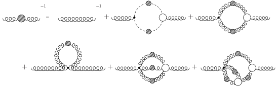
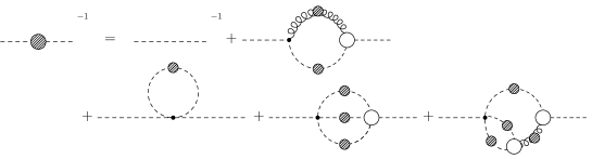
Figure 1: The coupled gluon and ghost Dyson–Schwinger equations from a BRS and Anti-BRS symmetric Lagrangean. Each equation contains one-loop diagrams, a tadpole contribution and a sunset and a squint diagram.

Both equations are shown diagrammatically in fig. 1. One clearly sees the striking similarity between the ghost and the gluon equation once a four-ghost interaction has been introduced. Both equations have bare and one loop parts, a tadpole contribution, a sunset and a squint diagram.

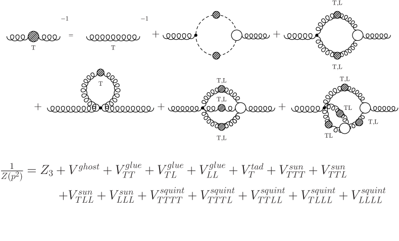
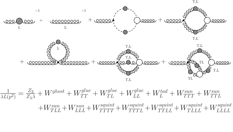
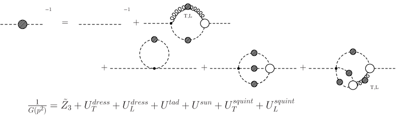
Figure 2: Various contributions from the respective diagrams in the transverse and longitudinal gluon equation and the equation for the ghost dressing function.

In order to sort the various contributions of the gluon equation to the inverse of the gluon propagator on the left hand side we project the equation on its longitudinal and transverse parts. It is well known that for linear covariant gauges, $\alpha=0$, the longitudinal part of the gluon propagator remains undressed Alkofer:2001wg . However, away from linear covariant gauges this is not the case as can be seen from the corresponding Slavnov-Taylor identity derived in Baulieu:1982sb . We then have three dressing functions in the general case and the propagators are given by

$$D_{\mu\nu}(p) = \left[D_{\mu\nu}(p)\right]_{T}+\left[D_{\mu\nu}(p)\right]_{L}$$ (32)

$$= \left(\delta_{\mu\nu}-\frac{p_{\mu}p_{\nu}}{p^{2}}\right)\frac{Z(p^{2})}{p^{2}}+\lambda L(p^{2})\frac{p_{\mu}p_{\nu}}{p^{4}},$$

$$D_{G}(p) = -\frac{G(p)}{p^{2}}.$$ (33)

The transversal and longitudinal gluon dressing functions $Z(p^{2})$ and $L(p^{2})$ can be extracted by contracting the gluon equation with the transversal and longitudinal projector respectively. The results are given graphically in fig. 2, where we also specify our notation for the different contributions being analyzed in the next section. Contributions in the transversal part of the gluon equation are denoted by the symbol $V$, contributions in the longitudinal part by $W$ and the ones in the ghost equation by $U$. The subscripts $T$ and $L$ indicate the respective parts of the gluon propagator running around in the loops of the diagrams and abbreviations for the diagrams are used. For example the symbol $W^{sun}_{LLT}$ denotes a contribution from the sunset diagram to the longitudinal gluon equation with two longitudinal and one transverse part of the gluon propagator running in the loop. To isolate the dressing functions the left hand side of the equations have already been divided by factors of $3p^{2}$ and $p^{2}$ respectively.

II.4 Generalized Slavnov–Taylor Identities

To derive the generalization of the Slavnov–Taylor identity for the longitudinal gluon propagator we start from the following BRS variations:

$$s_{r}\big{(}\partial A^{a}_{x}\bar{c}^{b}_{y}\big{)} = -\widetilde{Z}_{3}\,(\partial D_{r}c)^{a}_{x}\,\bar{c}^{b}_{y}\,+\,\partial A^{a}_{x}\,\big{(}B-\widetilde{Z}_{1}\,\frac{\alpha}{2}\,(\bar{c}\times c)\big{)}^{b}_{y}\;,$$ (34)

$$\bar{s}_{r}\big{(}\partial A^{a}_{x}c^{b}_{y}\big{)} = -\widetilde{Z}_{3}\,(\partial D_{r}\bar{c})^{a}_{x}\,c^{b}_{y}\,-\,\partial A^{a}_{x}\,\big{(}B+\widetilde{Z}_{1}\,(1-\frac{\alpha}{2})\,(\bar{c}\times c)\big{)}^{b}_{y}\;.$$ (35)

The corresponding vacuum expectation values vanish, and taking combinations of the expectation values of these equations we obtain:

$$0 = (1-\frac{\alpha}{2})\,\langle\,s_{r}\big{(}\partial A^{a}_{x}\bar{c}^{b}_{y}\big{)}\,\rangle\,-\,\frac{\alpha}{2}\,\langle\,\bar{s}_{r}\big{(}\partial A^{a}_{x}c^{b}_{y}\big{)}\,\rangle$$ (36)

$$= -\widetilde{Z}_{3}\,(1-\frac{\alpha}{2})\,\langle\,(\partial D_{r}c)^{a}_{x}\,\bar{c}^{b}_{y}\,\rangle\,+\,\widetilde{Z}_{3}\,\frac{\alpha}{2}\,\langle\,(\partial D_{r}\bar{c})^{a}_{x}\,c^{b}_{y}\,\rangle\,+\,\langle\,\partial A^{a}_{x}\,B^{b}_{y}\,\rangle\;.$$

Upon insertion of the e.o.m. of the $B$-field, $Z_{\lambda}\lambda\,B\,=\,iZ_{3}\partial A$, this directly leads to Eq. (27). On the other hand, the ghost DSEs from Eqs. (13) and (14) allow to eliminate the first two terms on the r.h.s., multiplying to them appropriate factors of $\frac{\alpha}{2}$ and $1-\frac{\alpha}{2}$ and inserting these expression in eq. (36) yields

$${Z_{3}}\,\langle\,\partial A^{a}_{x}\,\partial A^{b}_{y}\,\rangle = {Z_{\lambda}\,\lambda}\,\Big{\{}\,\delta^{ab}\delta_{xy}$$

$$- \,i\widetilde{Z}_{1}\,\frac{\alpha}{2}(1-\frac{\alpha}{2})\,\langle\,(\partial A\times c)^{a}_{x}\,\bar{c}^{b}_{y}\,\rangle\,+\,\frac{Z_{\lambda}\,\lambda}{Z_{3}}\,\widetilde{Z}_{1}^{2}\,\frac{\alpha}{2}(1-\frac{\alpha}{2})^{2}\,\langle\,\big{(}(\bar{c}\times c)\times c\big{)}^{a}_{x}\,\bar{c}^{b}_{y}\,\rangle$$

$$+ \,i\widetilde{Z}_{1}\,\frac{\alpha}{2}(1-\frac{\alpha}{2})\,\langle\,(\partial A\times\bar{c})^{a}_{x}\,c^{b}_{y}\,\rangle\,+\,\frac{Z_{\lambda}\,\lambda}{Z_{3}}\,\widetilde{Z}_{1}^{2}\,\frac{\alpha^{2}}{4}(1-\frac{\alpha}{2})\,\langle\,\big{(}(\bar{c}\times c)\times\bar{c}\big{)}^{a}_{x}\,c^{b}_{y}\,\rangle\,\Big{\}}\;.$$

This generalizes the Slavnov–Taylor identity for the longitudinal part of the gluon propagator which, contrary to the standard Faddeev–Popov gauges, does in general acquire renormalization by the interactions, c.f. Eq. (7). On the r.h.s. of the Slavnov–Taylor identity, the terms in the 3rd line are the Faddeev–Popov conjugate of those in the 2nd. In the ghost anti-ghost symmetric case for $\alpha\!=\!1$ they are identical. In this case the Slavnov–Taylor identity simplifies,

$${Z_{3}}\,\langle\,\partial A^{a}_{x}\,\partial A^{b}_{y}\,\rangle\,=\,{Z_{\lambda}\,\lambda}\,\Big{\{}\,\delta^{ab}\delta_{xy}\,-\,i\widetilde{Z}_{1}\,\frac{1}{2}\,\langle\,(\partial A\times c)^{a}_{x}\,\bar{c}^{b}_{y}\,\rangle\,+\,\frac{Z_{\lambda}\,\lambda}{Z_{3}}\,\frac{{\widetilde{Z}}_{1}^{2}}{4}\,\langle\,\big{(}(\bar{c}\times c)\times c\big{)}^{a}_{x}\,\bar{c}^{b}_{y}\,\rangle\,\Big{\}}\;.$$ (38)

Note that close to the Landau gauge the corrections to the unity of the standard Faddeev–Popov gauges are suppressed by one order in the gauge parameter $\lambda$.

A further Slavnov–Taylor identity is obtained by adding the expectation values of the BRS variations in Eqs. (34) and (35):

$$0 = \langle\,s_{r}\big{(}\partial A^{a}_{x}\bar{c}^{b}_{y}\big{)}\,\rangle\,+\,\langle\,\bar{s}_{r}\big{(}\partial A^{a}_{x}c^{b}_{y}\big{)}\,\rangle$$ (39)

$$= -\widetilde{Z}_{3}\,\langle\,(\partial D_{r}c)^{a}_{x}\,\bar{c}^{b}_{y}\,\rangle\,-\,\widetilde{Z}_{3}\,\langle\,(\partial D_{r}\bar{c})^{a}_{x}\,c^{b}_{y}\,\rangle\,-\,\widetilde{Z}_{1}\,\langle\,\partial A^{a}_{x}\,(\bar{c}\times c)^{b}_{y}\,\rangle\;.$$

This leads to Eq. (26) as promised in the previous subsection.

These Slavnov–Taylor identities indicate that the Landau gauge limit $\lambda\to 0$ is smooth. Based on Eqs. (II.4) and (39) one may anticipate that an infrared massless-like longitudinal part of the gluon propagator leads for sufficiently small values of the gauge parameter $\lambda$ to the same infrared enhancement of ghosts as observed in the Landau gauge.

III Infrared analysis with bare vertices for arbitrary gauge parameters

In this section we will analyse the behaviour of the two-point functions at small momenta $p^{2}$. We will employ a truncation scheme that successfully has been applied in the case of Landau gauge Lerche:2002ep ; Zwanziger:2001kw ; Fischer:2002hn and explore its applicability to general gauges.

An interesting result of the investigations in Landau gauge is the observation, that there is no qualitative difference of the solutions found with bare vertices or with vertices dressed by the use of Slavnov–Taylor identities. This has not only been found in truncations using angular approximations vonSmekal:1997is ; Atkinson:1998tu for the integrals, but has been confirmed recently for a range of possible vertex dressings in a truncation scheme without any angular approximations Lerche:2002ep . The reason for this somewhat surprising result has been attributed to the non-renormalization of the ghost-gluon vertex in Landau gauge, that is $\tilde{Z}_{1}=1$. It seems as if the violation of gauge invariance using a bare vertex is not that severe in Landau gauge such that the resulting equations still provide meaningful results. In the following we will explore to what extent such a simple truncation idea is applicable in other gauges where $\tilde{Z}_{1}\not=1$.

In Landau gauge the coupled set of Dyson-Schwinger equations is solved by pure power laws for the ghost and gluon dressing functions. Such solutions are determined analytically by plugging a power law ansatz in the equations and match appropriate powers on the left and right hand side. Once several power solutions have been found the remaining task is to single out the one matching the numerical solution of the renormalized equation. In Landau gauge it has been shown that indeed only one of the power solutions found in refs. Lerche:2002ep ; Zwanziger:2001kw is the correct infrared limit of the renormalized solution Fischer:2002hn by solving the equations numerically for all momenta. In the following we will investigate whether there are power solutions at all using bare vertices for general gauge parameter $\alpha$ and $\lambda$.

Now we employ the power law ansatz for the dressing functions,

$$G(x)=Bx^{\beta},\>\>\>\>Z(x)=Ax^{\sigma},\>\>\>\>L(x)=Cx^{\rho},$$ (40)

where $x=p^{2}$ has been used. Together with the expressions for the bare vertices given in appendix B we plug the power laws into the ghost and the gluon equation. The formulae for the various integrals are given in appendix C. The straightforward but tedious algebra is done with the help of the algebraic manipulation program FORM Form . In ref. Lerche:2002ep it has been shown that the renormalization functions $Z_{3}$ and $\tilde{Z}_{3}$ do not play a role in the determination of possible power solutions of the equations in the infrared region of momentum. Furthermore the tadpoles just give constant contributions to the respective propagators which vanish in the process of renormalization. Thus we safely omit them in the present investigation.

For the most general gauges, $\alpha\neq 0$ and $\lambda\neq 0$, we obtain the following structure:

$$B^{-1}x^{-\beta} = x^{\sigma+\beta}(U^{\prime})^{dress}_{T}+x^{\rho+\beta}(U^{\prime})^{dress}_{L}+x^{3\beta}(U^{\prime})^{sun}$$ (41)

$$+x^{\sigma+3\beta}(U^{\prime})^{squint}_{T}+x^{\rho+3\beta}(U^{\prime})^{squint}_{L}$$

$$A^{-1}x^{-\sigma} = x^{2\beta}(V^{\prime})^{ghost}+x^{2\sigma}(V^{\prime})^{glue}_{TT}+x^{\sigma+\rho}(V^{\prime})^{glue}_{TL}+x^{2\rho}(V^{\prime})^{glue}_{LL}$$ (42)

$$+x^{3\sigma}(V^{\prime})^{sun}_{TTT}+x^{2\sigma+\rho}(V^{\prime})^{sun}_{TTL}+x^{\sigma+2\rho}(V^{\prime})^{sun}_{TLL}+x^{3\rho}(V^{\prime})^{sun}_{LLL}$$

$$+x^{4\sigma}(V^{\prime})^{squint}_{TTTT}+x^{3\sigma+\rho}(V^{\prime})^{squint}_{TTTL}+x^{2\sigma+2\rho}(V^{\prime})^{squint}_{TTLL}$$

$$+x^{\sigma+3\rho}(V^{\prime})^{squint}_{TLLL}+x^{4\rho}(V^{\prime})^{squint}_{LLLL}$$

$$\left(C\lambda\right)^{-1}x^{-\rho} = +x^{2\beta}(W^{\prime})^{ghost}+x^{2\sigma}(W^{\prime})^{glue}_{TT}+x^{\sigma+\rho}(W^{\prime})^{glue}_{TL}$$ (43)

$$+x^{3\sigma}(W^{\prime})^{sun}_{TTT}+x^{2\sigma+\rho}(W^{\prime})^{sun}_{TTL}+x^{\sigma+2\rho}(W^{\prime})^{sun}_{TLL}+x^{3\rho}(W^{\prime})^{sun}_{LLL}$$

$$+x^{4\sigma}(W^{\prime})^{squint}_{TTTT}+x^{3\sigma+\rho}(W^{\prime})^{squint}_{TTTL}+x^{2\sigma+2\rho}(W^{\prime})^{squint}_{TTLL}$$

$$+x^{\sigma+3\rho}(W^{\prime})^{squint}_{TLLL}.$$

Here the primed quantities are momentum independent functions of $\beta$, $\sigma$ and $\rho$, c.f. fig. 2 where the corresponding unprimed, momentum dependent quantities have been introduced. The pattern of the equation is such that each primed factor on the right hand side is accompanied by the squared momentum $x$ to the power of the dressing function content of the respective diagram. In appendix D we demonstrate how such a pattern emerges for example from the sunset diagram in the ghost equation, $(U)^{sun}$. Note that the contributions $(W^{\prime})^{glue}_{LL}$ and $(W^{\prime})^{squint}_{LLLL}$ are zero and therefore missing in the longitudinal gluon equation (43) as momentum conservation cannot hold with three longitudinal gluons in the three gluon vertex.

For the following argument we focus on one particular contribution on each right hand side of the equations:

$$B^{-1}x^{-\beta} = x^{3\beta}(U^{\prime})^{sun}+\ldots$$ (44)

$$A^{-1}x^{-\sigma} = x^{4\sigma}(V^{\prime})^{squint}_{TTTT}+\ldots$$ (45)

$$\left(C\lambda\right)^{-1}x^{-\rho} = x^{3\rho}(W^{\prime})^{sun}_{LLL}+\ldots$$ (46)

The coefficients $(U^{\prime})^{sun}$, $(V^{\prime})^{squint}_{TTTT}$ and $(W^{\prime})^{sun}_{LLL}$ are nonzero and explicitly given in appendix D. First it is now easy to see from equations (44), (45) and (46) that neither $\beta$ nor $\sigma$ nor $\rho$ can be negative. If one of these powers would be negative the limit $x\rightarrow 0$ would lead to a vanishing left hand side of the respective equation whereas the right hand side is singular in this limit. This is a contradiction as the power on the left hand side of the equation should match the leading power on the right hand side. Second if one of $\beta$, $\sigma$ or $\rho$ would be positive, then the diverging left hand side of the respective equation would require a diverging counterpart on the right hand side. However, all powers on the right hand side are positive as we already concluded that $\beta$, $\sigma$ or $\rho$ are not negative and there are no minus sines in any powers on the right hand sides, c.f. Eqs. (41), (42) and (43)). Therefore for positive powers all terms on the right hand side vanish in the limit $x\rightarrow 0$ which leads again to a contradiction. The last possibility is then $\beta=\sigma=\rho=0$, but then one gets perturbative logarithms on the right hand side of the equation which do not match the constant on the left hand side. Thus in the all-bare-vertex truncation there is no power solution for general values of the gauge parameters $\lambda\not=0$ and $\alpha\not=0$. Based on the considerations on the Slavnov–Taylor identities given in the previous section we therefore arrive at the conclusion that this truncation is insufficient to determine the infrared behaviour of the propagators even qualitatively.

There are two limits for the gauge parameters $\alpha$ and $\lambda$ in which the situation changes. The first one is $\alpha=0$, that is ordinary linear covariant gauges. Due to the corresponding Slavnov–Taylor identity the longitudinal part of the gluon propagator remains undressed, $L(p^{2})=1$ Alkofer:2001wg . However, replacing dressed vertices by bare ones in the infrared, this identity might be violated (which does not happen in perturbation theory, of course). We therefore employ the general expression $L(p^{2})=C(p^{2})^{\rho}$ for the longitudinal gluon dressing function and explore whether the limit $\rho\rightarrow 0$ can be taken with bare vertices. In the ghost equation the squint as well as the sunset diagram disappear and we are left with the one-loop contributions $U^{dress}_{T}$ and $U^{dress}_{L}$. The explicit expression for the ghost equation is given by (cf. appendix D)

$$B^{-1}x^{-\beta} = U^{dress}_{T}+U^{dress}_{L}$$ (48)

$$= x^{(\beta+\sigma)}\frac{g^{2}N_{c}\tilde{Z}_{1}AB}{16\pi^{2}}\,\frac{-3}{2\,(\beta+\sigma)\,(-1+\beta+\sigma)}\frac{\Gamma(2+\beta)\,\Gamma(1+\sigma)\,\Gamma(2-\beta-\sigma)}{\Gamma(1-\beta)\,\Gamma(2-\sigma)\,\Gamma(3+\beta+\sigma)}$$

$$-x^{(\beta+\rho)}\frac{g^{2}N_{c}\tilde{Z}_{1}\lambda BC}{16\pi^{2}}\>\>\frac{\rho+1/2}{\beta}\>\>\frac{\Gamma(2+\beta)\Gamma(1+\rho)\Gamma(-\beta-\rho)}{\Gamma(-\beta)\Gamma(2-\rho)\Gamma(3+\rho+\beta)}\,.$$

For $\rho\rightarrow 0$ we run into the same contradiction as explained above for general values of the gauge parameters $\alpha$ and $\lambda$. However, admitting the generation of a (spurious) longitudinal gluon dressing this contradiction can be resolved in the following way: Equation (45) for the transversal gluon dressing function does not change in structure, therefore $\sigma>0$. Furthermore we have $\rho>0$ from eq. (46). Then we have $-2\beta=\sigma$ and/or $-2\beta=\rho$ in the ghost equation (48) and $\beta<0$, i.e. a diverging ghost dressing function in the infrared. From this it follows immediately, that the ghost loop is the dominant contribution in both, the equations for the transversal and longitudinal gluon dressing function. From these two equations we therefore infer

$$-\beta=\sigma/2=\rho/2=:\kappa\,,$$ (49)

which is consistent with the ghost equation. We thus find an infrared vanishing gluon dressing and a singular ghost dressing function for all values of the gauge parameter $\lambda$. This result is identical to the one in Landau gauge Zwanziger:2001kw ; Lerche:2002ep ; Fischer:2002hn . However, a word of caution is in order. In Landau gauge there are indications vonSmekal:1997is ; Watson:2001yv that the general result (49) does not change when the vertices are dressed. This has been confirmed recently for a range of possible vertex dressings Lerche:2002ep . It is an as yet open question whether this is true for $\lambda\neq 0$ in the same way.

Having addressed the case of linear covariant gauges with $\alpha=0$ we now turn to the other interesting limit, that is $\lambda=0$, while $\alpha\neq 0$. It is easy to see, that the $\alpha$-dependence of the Lagrangean (1) can be eliminated in this case by partial integration using the constraint $\partial A=0$. However, on the level of the DSEs with bare vertices there remain spurious $\alpha$-dependent terms on the right hand side of the gluon equation. In the next section we will investigate the dependence of the Landau gauge solution on these spurious $\alpha$-terms.

IV Solutions in Landau gauge

To assess the influence of the spurious $\alpha$-terms in Landau gauge we use the truncation scheme developed in Fischer:2002hn . There the two loop diagrams in the gluon equation have been neglected as they are subleading in the perturbative regime and ghost loop dominance has been assumed in the infrared. In order to obtain the correct one loop behaviour of the ghost and gluon dressing functions the gluon loop has been modified by replacing the renormalization constant $Z_{1}$ by a momentum dependent function $\mathcal{Z}_{1}$:

$$Z_{1}(L,s)\to{\cal Z}_{1}(x,y,z;s,L)=\frac{G(y)^{(-2-6\delta)}}{Z(y)^{(1+3\delta)}}\frac{G(z)^{(-2-6\delta)}}{Z(z)^{(1+3\delta)}}$$ (50)

Here $L=\Lambda^{2}$ denotes a cutoff and $s=\mu^{2}$ a renormalization scale in units of squared momenta. The momentum $x=p^{2}$ is the one flowing into the loop, $y=q^{2}$ is the loop momentum over which is integrated and $z:=k^{2}=(p-q)^{2}$. Furthermore the anomalous dimension $\delta$ of the ghost dressing function has been used. The gluon equation is contracted with the general tensor

$${\mathcal{P}}^{(\zeta)}_{\mu\nu}(p)=\delta_{\mu\nu}-\zeta\frac{p_{\mu}p_{\nu}}{p^{2}}\,.$$ (51)

As a completely transversal gluon equation would be independent of the parameter $\zeta$ the use of the general projector provides an opportunity to test for violations of transversality due to the truncation. For $\zeta\not=4$ one has to take care of spurious quadratic divergencies that have to be subtracted in the kernel of the gluon equation.

The coupled set of equations for the ghost and gluon dressing functions then read as follows

$$\frac{1}{G(x)} = Z_{3}-g^{2}N_{c}\int\frac{d^{4}q}{(2\pi)^{4}}\frac{K(x,y,z)}{xy}G(y)Z(z)\;,$$ (52)

$$\frac{1}{Z(x)} = \tilde{Z}_{3}+g^{2}\frac{N_{c}}{3}\int\frac{d^{4}q}{(2\pi)^{4}}\frac{M(x,y,z)}{xy}G(y)G(z)$$ (53)

$$\qquad+g^{2}\frac{N_{c}}{3}\int\frac{d^{4}q}{(2\pi)^{4}}\frac{Q(x,y,z)}{xy}Z(y)Z(z){\cal Z}_{1}(y,z)\;.$$

The kernels ordered with respect to powers of $z:=p^{2}=(k-q)^{2}$ have the form:

$$K(x,y,z) = \frac{1}{z^{2}}\left(-\frac{(x-y)^{2}}{4}\right)+\frac{1}{z}\left(\frac{x+y}{2}\right)-\frac{1}{4}$$ (54)

$$M(x,y,z) = \frac{1}{z}\left(\frac{(\zeta-1)\alpha^{2}-(\zeta-1)2\alpha+\zeta-2}{4}x+\frac{y}{2}-\frac{\zeta}{4}\frac{y^{2}}{x}\right)+\frac{1}{2}+\frac{\zeta}{2}\frac{y}{x}-\frac{\zeta}{4}\frac{z}{x}$$ (55)

$$Q(x,y,z) = \frac{1}{z^{2}}\left(\frac{1}{8}\frac{x^{3}}{y}+x^{2}-\frac{19-\zeta}{8}xy+\frac{5-\zeta}{4}y^{2}+\frac{\zeta}{8}\frac{y^{3}}{x}\right)$$ (56)

$$+\frac{1}{z}\left(\frac{x^{2}}{y}-\frac{15+\zeta}{4}x-\frac{17-\zeta}{4}y+\zeta\frac{y^{2}}{x}\right)$$

$$-\left(\frac{19-\zeta}{8}\frac{x}{y}+\frac{17-\zeta}{4}+\frac{9\zeta}{4}\frac{y}{x}\right)$$

$$+z\left(\frac{\zeta}{x}+\frac{5-\zeta}{4y}\right)+z^{2}\frac{\zeta}{8xy}+\frac{5}{4}(4-\zeta).$$

      

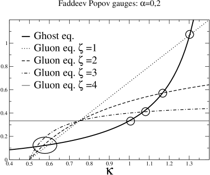
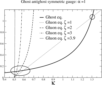
Figure 3: Here the graphical solution to equation (58) is shown. The thick line represents the left hand side of equation (58), whereas the other curves depict the right hand side for different values of the parameters $\zeta$. The left figure shows results for $\alpha=0$ and $\alpha=2$, whereas in the figure on the right $\alpha=1$. The ellipse marks the bulk of solutions between $\kappa=0.5$ and $\kappa=0.6$ for $\zeta=1$, whereas the circles in the left figure show the movement of the solution for the Brown-Pennington case $\zeta=4$ from $\kappa=1$ to $\kappa=1.3$.

First we accomplish the infrared analysis. With equation (49) we employ the ansatz

$$Z(x)=Ax^{2\kappa}\>\>\>\>\>\>\>G(x)=Bx^{-\kappa}$$ (57)

in the equations (52) and (53). After integration we match coefficients of equal powers on both side of the equations and obtain

$$\frac{1}{18}\frac{(2+\kappa)(1+\kappa)}{(3-2\kappa)}$$

$$=\frac{(4\kappa-2)\,(-1+\kappa)}{(\zeta-1)\left[4\,\kappa^{2}\,(\alpha^{2}-2\,\alpha+1)+8\,\kappa\,\alpha\,(2-\alpha)+3\,\alpha\,(\alpha-2)\right]+\kappa\,(10-7\,\zeta)-6+3\,\zeta}\;.$$

(58)

The values of $\kappa$ for different projectors $\mathcal{P}^{(\zeta)}$ can be read off fig. 3. The curve given by the fully drawn line represents the term on the left hand side of equation (58), whereas the other lines depict the right hand side for several values of the parameter $\zeta$. Only the two $\zeta=1$ solutions are manifestly independent of $\alpha$, as pointed out in Lerche:2002ep . The spurious $\alpha$-dependence of the $\zeta=4$ values reported therein, here implies that general $\zeta$ solutions must necessarily show such an $\alpha$-dependence also, whenever $\zeta\not=1$. However, the bulk of solutions between $\kappa=0.5$ and $\kappa=0.6$ remains nearly unchanged when $\alpha$ is varied, whereas most of the solutions for $\kappa\geq 1$ disappear. For the Brown-Pennington projector $\zeta=4$ no solution can be found for the symmetric case, $\alpha=1$, in complete agreement with the findings of ref. Lerche:2002ep . Indeed it has been shown Fischer:2002hn that only the smaller solutions are those that connect to numerical results for finite momenta.

         

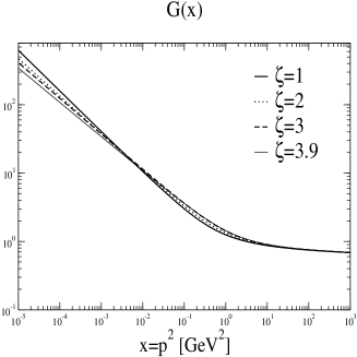
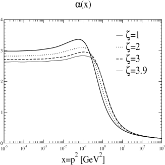
Figure 4: Shown are the gluon dressing function, the ghost dressing function and the running coupling in the truncation scheme Fischer:2002hn for the gauge parameters $\alpha=1$ and $\lambda=0$ and different projectors $\mathcal{P}^{(\zeta)}$.

We now explore the impact of the spurious $\alpha$ term on the behaviour of the solutions for all momenta $x$. We have solved eqs. (52) and (53) numerically using the same technique as described in Fischer:2002hn . The results can be seen in fig. 4. As the dependence of the kernel of the ghost loop on $\alpha$ vanishes in the case of the transverse projector, $\zeta=1$, this solution is the same as the one already calculated in Fischer:2002hn . For the other cases the power $\kappa$ changes from $0.5953$ for $\zeta=1$ to $0.5020$ for $\zeta=3.9$ in accordance with the infrared analysis. The ultraviolet properties of the solutions are slightly disturbed compared to the cases $\alpha=0$ and $\alpha=2$. An analysis of the ultraviolet behaviour done similarly to the one in ref. Fischer:2002hn reveals that the $\alpha$-term in the ghost loop induces a spurious dependence of the anomalous dimensions on the parameter $\zeta$:

$$\gamma = \frac{-26-(\zeta-1)\alpha(2-\alpha)}{44+(\zeta-1)\alpha(2-\alpha)}$$

$$\delta = \frac{-9}{44+(\zeta-1)\alpha(2-\alpha)}.$$ (59)

For general $\alpha$ only the transverse projector removes the spurious term in the ghost equation and leads to the correct one loop scaling of the equations, that is $\delta=-9/44$ for the ghost and $\gamma=-13/22$ for the gluon dressing function for an arbitrary number of colors and zero flavours.

V Conclusion

We have studied the infrared behaviour of the ghost and gluon propagators in general covariant gauges. These gauges allow to interpolate via a second gauge parameter between the linear-covariant ones of standard Faddeev-Popov theory and the ghost-antighost symmetric gauges. We derived the corresponding generalised Dyson–Schwinger equations for the propagators which include the ones of linear-covariant gauges as the limit where the second gauge parameter vanishes. Note that ghost-antighost symmetric gauges are particularly interesting as they allow an interpretation of the antighost field being the antiparticle of the ghost which includes also the possibility of ghost-antighost condensate. Due to the emergence of a four-ghost interaction term in the Lagrangean for general values of gauge parameters the Dyson–Schwinger equation of the ghost propagator displays a rich structure very similar to the one of the gluon equation. On the other hand, in the gluon equation we obtain the same structure as in linear covariant gauges apart from the fact that the gluon propagator acquires a nontrivial longitudinal part which appears in turn in all diagrams. The gluon and ghost equations depend therefore on three dressing functions, one for the ghost, one for the transverse part of the gluon propagator and one for the longitudinal one, which are constrained, however, by Slavnov-Taylor identities in an intricate way.

We then employed a truncation scheme for the Dyson–Schwinger equations that uses bare vertices in place of the dressed ones. The success of this particular truncation scheme in Landau gauge has been attributed to the non-renormalization of the ghost-gluon vertex, that is $\widetilde{Z}_{1}=1$. We addressed the infrared behaviour of the ghost and gluon propagators for general gauges by employing power law ansätze for the respective dressing functions. We then have been able to evaluate the infrared behavior of the gluon and ghost equations analytically.

For all linear covariant gauges we find a similar result as compared to the one in Landau gauge: An infrared suppressed gluon propagator and an infrared enhanced ghost. Whereas in Landau gauge there are indications that this generic result is not changed when the vertices are dressed Lerche:2002ep , it remains an open question whether this is the case in linear covariant gauges in general. Away from linear covariant gauges, that is in the general case $\alpha\not=0$ and $\lambda\not=0$, we do not find power solutions for the dressing functions. However, we expect this to change with appropriate vertex dressings. Nevertheless, it remains to be emphasized that therefore also the occurrence of a ghost and/or gluon mass is excluded in this specific truncation scheme within this class of gauges. A Dyson–Schwinger equation based investigation of the related question of a ghost-antighost vacuum condensate, or more generally, of an ‘on-shell’-BRS-invariant dimension two condensate, needs to take into account the generalized Slavnov–Taylor identities (II.4) and (39). The question arises whether an infrared massless-like longitudinal part of the gluon propagator leads for all values of the gauge parameters to the same infrared enhancement of ghosts as observed in the Landau gauge. Work in this direction is in progress.

A special case among all gauges considered here is Landau gauge. In the limit $\lambda=0$ the general Lagrangean (1) becomes independent of the second gauge parameter $\alpha$, thus Landau gauge is also a special case of ghost-antighost symmetric gauges. Although the Lagrangean of the theory is independent of the gauge parameter $\alpha$, our simple truncation scheme breaks this invariance and spurious $\alpha$-dependent terms arise in the ghost loop of the gluon Dyson–Schwinger equation. Examining the case $\alpha=1$ we showed that the influence of these spurious terms is very small. We determined solutions for the ghost and gluon dressing functions both analytically in the infrared and numerically for finite momenta and found solutions identical to the ones of ref. Fischer:2002hn provided the gluon equation is projected onto its physical, transversal components. We thus recovered the results of Landau gauge from a different direction in the two dimensional space of gauge parameters.

VI Acknowledgments

We are grateful to Jacques Bloch for checking our FORM code with some of his results. Furthermore we are indebted to Herbert Weigel for pointing out an inconsistency in the original version of the manuscript. This work has been supported by the DFG under contracts Al 279/3-3, Al 279/3-4, SM 70-1/1 and Re 856-5/1 and by the contract GRK683 (European graduate school Basel–Tübingen).

Appendix A Appendix A: Derivation of the Dyson–Schwinger equation for the Ghost Propagator

We start by transforming the Lagrangean (1) into a more suitable form by partial integration, assuming the usual boundary conditions of vanishing fields at infinity. In order to keep notation on a readable level we will suppress renormalization constants in this appendix: The derivation of the Dyson–Schwinger equation for the ghost propagator remains formally unchanged by the rescaling (5) and thus the appropriate renormalization constants can be regained straightforwardly. We obtain

$$\cal{L} = \frac{1}{2}A_{\mu}^{a}\left(-\partial^{2}\delta_{\mu\nu}+\left(1-\frac{1}{\lambda}\right)\partial_{\mu}\partial_{\nu}\right)A_{\nu}^{a}-gf^{abc}\left(\partial_{\mu}A_{\nu}^{a}\right)A_{\mu}^{b}A_{\nu}^{c}$$ (60)

$$+\frac{g^{2}}{4}f^{abe}f^{cde}A_{\mu}^{a}A_{\nu}^{b}A_{\mu}^{c}A_{\nu}^{d}+\bar{c}^{a}\partial^{2}c^{a}+\frac{\alpha}{2}\left(1-\frac{\alpha}{2}\right)\frac{\lambda}{2}g^{2}f^{ace}f^{bde}\bar{c}^{a}\bar{c}^{b}c^{c}c^{d}$$

$$+i\left(1-\frac{\alpha}{2}\right)gf^{abc}\bar{c}^{a}\partial_{\mu}\left(A_{\mu}^{c}c^{b}\right)+i\frac{\alpha}{2}gf^{abc}\bar{c}^{a}A_{\mu}^{c}\partial_{\mu}c^{b}.$$

The partition function of the theory is given by

$$Z[J,\sigma,\bar{\sigma}]=\int{\cal D}[A\bar{c}c]\exp\left\{-\int d^{4}z\,{\cal{L}}+\int d^{4}z\,\left(A^{a}J^{a}+\bar{\sigma}c+\bar{c}\sigma\right)\right\}$$ (61)

with the sources $J$, $\sigma$ and $\bar{\sigma}$ of the gluon, antighost and ghost fields, respectively. The action is given by $\mathcal{S}[J,c,\bar{c}]=\int d^{4}z\,{\cal{L}}$. The generating functional of connected Green’s functions, $W[J,\sigma,\bar{\sigma}]$, is defined as the logarithm of the partition function. The functional Legendre transform of $W$ is the effective action

$$\Gamma[A,\bar{c},c]=-W[J,\sigma,\bar{\sigma}]+\int d^{4}z\left(A^{a}J^{a}+\bar{\sigma}c+\bar{c}\sigma\right),$$ (62)

which is the generating functional of one-particle irreducible vertex functions. The fields and sources can be written as functional derivatives of the respective generating functionals in the following way

$$\frac{\delta W}{\delta\sigma} = \bar{c},\hskip 28.45274pt\frac{\delta W}{\delta\bar{\sigma}}=c,\hskip 28.45274pt\frac{\delta W}{\delta J_{\mu}}=A_{\mu},$$

$$\frac{\delta\Gamma}{\delta c} = \bar{\sigma},\hskip 28.45274pt\frac{\delta\Gamma}{\delta\bar{c}}=\bar{\sigma},\hskip 28.45274pt\frac{\delta\Gamma}{\delta A_{\mu}}=J_{\mu}.$$ (63)

The sign conventions have been chosen such that derivatives with respect to $\bar{c}$ and $\bar{\sigma}$ are left derivatives whereas the ones with respect to ${c}$ and ${\sigma}$ are right derivatives,

$$\frac{\delta}{\delta\left(\bar{\sigma},\bar{c}\right)}:=\mbox{left derivative}\hskip 28.45274pt\frac{\delta}{\delta\left({\sigma},{c}\right)}:=\mbox{right derivative}.$$ (64)

Given that the functional integral is well-defined, the Dyson-Schwinger equation for the ghost propagator is derived from the observation that the integral of a total derivative vanishes provided the measure is invariant under field translations. We take the derivative with respect to the antighost field and obtain

$$0 = \int{\cal D}[A\bar{c}c]\frac{\delta}{\delta\bar{c}}\exp\left\{-\int d^{4}z\,{\cal{L}}+\int d^{4}z\,\left(A^{a}J^{a}+\bar{\sigma}c+\bar{c}\sigma\right)\right\}$$ (65)

$$= \int{\cal D}[A\bar{c}c]\left(-\frac{\delta S\left[A,c,\bar{c}\right]}{\delta\bar{c}}+\sigma\right)\exp\left\{-\int d^{4}z\,{\cal{L}}+\int d^{4}z\,\left(A^{a}J^{a}+\bar{\sigma}c+\bar{c}\sigma\right)\right\}$$

$$= \left(-\frac{\delta S\left[\frac{\delta}{\delta J},\frac{\delta}{\delta\bar{\sigma}},\frac{\delta}{\delta\sigma}\right]}{\delta\bar{c}}+\sigma\right)Z[J,\sigma,\bar{\sigma}].$$

Now we use the relations (63) and apply a further functional derivative with respect to the source $\sigma^{b}(y)$. We arrive at

$$0=\left(-\frac{\delta S}{\delta\bar{c}^{c}(z)}\bar{c}^{b}(y)+\sigma^{c}(z)\bar{c}^{b}(y)+\delta(z-y)\delta_{cb}\right)Z[J,\sigma,\bar{\sigma}]$$ (66)

with explicit colour indices and space-time arguments. Setting the sources equal to zero we obtain the ghost Dyson-Schwinger equation

$$\left\langle\frac{\delta S}{\delta\bar{c}^{c}(z)}\bar{c}^{b}(y)\right\rangle=\delta(z-y)\delta_{cb}.$$ (67)

The derivative is easily calculated

$$\frac{\delta S}{\delta\bar{c}^{c}(z)} = \partial^{2}c^{c}(z)+\frac{\alpha}{2}\left(1-\frac{\alpha}{2}\right)\frac{\lambda}{2}g^{2}f^{cde}f^{fge}\bar{c}^{d}(z)c^{f}(z)c^{g}(z)$$ (68)

$$+i\left(1-\frac{\alpha}{2}\right)gf^{cde}\partial_{\mu}\left(A^{e}_{\mu}(z)c^{d}(z)\right)+i\frac{\alpha}{2}gf^{cde}A^{e}_{\mu}(z)\partial_{\mu}c^{d}(z).$$

Whereas in the covariant formalism full and connected three-point functions are the same, the four-point correlations have to be decomposed into disconnected and connected parts. For the four-ghost correlation function this results in

$$\langle\bar{c}^{b}(y)\bar{c}^{d}(z)c^{f}(z)c^{g}(z)\rangle = \langle\bar{c}^{b}(y)c^{g}(z)\rangle\,\langle\bar{c}^{d}(z)c^{f}(z)\rangle-\langle\bar{c}^{b}(y)c^{f}(z)\rangle\,\langle\bar{c}^{d}(z)c^{g}(z)\rangle$$ (69)

$$+ \langle\bar{c}^{b}(y)\bar{c}^{d}(z)c^{f}(z)c^{g}(z)\rangle_{conn.}\,.$$

Keeping in mind the Grassmann nature of the ghost and antighost fields we then obtain

$$-\delta(z-y)\delta_{cb} = \partial^{2}\langle\bar{c}^{b}(y)c^{c}(z)\rangle+\frac{\alpha}{2}\left(1-\frac{\alpha}{2}\right)\frac{\lambda}{2}g^{2}f^{cde}f^{fge}\left\{\langle\bar{c}^{b}(y)\bar{c}^{d}(z)c^{f}(z)c^{g}(z)\rangle\right.$$

$$\left.+\left(\langle\bar{c}^{b}(y)c^{g}(z)\rangle\,\langle\bar{c}^{d}(z)c^{f}(z)\rangle-\langle\bar{c}^{b}(y)c^{f}(z)\rangle\,\langle\bar{c}^{d}(z)c^{g}(z)\rangle\right)\right\}$$

$$+ \left(1-\frac{\alpha}{2}\right)gf^{cde}\langle\bar{c}^{b}(y)\partial_{\mu}\left(A^{e}_{\mu}(z)c^{d}(z)\right)\rangle+\frac{\alpha}{2}gf^{cde}\langle\bar{c}^{b}(y)A^{e}_{\mu}(z)\partial_{\mu}c^{d}(z)\rangle\,,$$

where all correlations are connected Green’s functions. We now use the relation

$$\delta(y-x)\delta^{ab}=\frac{\delta\bar{\sigma}^{b}(y)}{\delta\bar{\sigma}^{a}(x)}=\int d^{4}z\frac{\delta\bar{\sigma}^{b}(y)}{\delta\bar{c}^{d}(z)}\frac{\delta\bar{c}^{d}(z)}{\delta\bar{\sigma}^{a}(x)} = \int d^{4}z\frac{\delta^{2}\Gamma}{\delta\bar{c}^{d}(z)\delta c^{b}(y)}\frac{\delta^{2}W}{\delta\bar{\sigma}^{a}(x)\delta\sigma^{d}(z)}$$

$$=: \int d^{4}z\left[D_{G}^{db}(z-y)\right]^{-1}D_{G}^{ad}(x-z)$$

and multiply eq. (LABEL:DSEa) with $-[D_{G}^{ac}(x-z)]^{-1}=\left[\langle\bar{c}^{c}(z)c^{a}(x)\rangle\right]^{-1}$. We arrive at

$$[D_{G}^{ab}(x-y)]^{-1} = \partial^{2}\delta(x-y)\delta^{ab}$$

$$- \frac{\alpha}{2}\left(1-\frac{\alpha}{2}\right)\frac{\lambda}{2}g^{2}f^{cde}f^{fge}\int d^{4}z\,[D_{G}^{ac}(x-z)]^{-1}\left\{\langle\bar{c}^{b}(y)\bar{c}^{d}(z)c^{f}(z)c^{g}(z)\rangle\right.$$

$$\hskip 68.28644pt+\,\left.\langle\bar{c}^{b}(y)c^{g}(z)\rangle\,\langle\bar{c}^{d}(z)c^{f}(z)\rangle-\langle\bar{c}^{b}(y)c^{f}(z)\rangle\,\langle\bar{c}^{d}(z)c^{g}(z)\rangle\right\}$$

$$- i\left(1-\frac{\alpha}{2}\right)gf^{cde}\int d^{4}z\,[D_{G}^{ac}(x-z)]^{-1}\langle\bar{c}^{b}(y)\partial_{\mu}\left(A^{e}_{\mu}(z)c^{d}(z)\right)\rangle$$

$$- i\frac{\alpha}{2}gf^{cde}\int d^{4}z\,[D_{G}^{ac}(x-z)]^{-1}\langle\bar{c}^{b}(y)A^{e}_{\mu}(z)\partial_{\mu}c^{d}(z)\rangle.$$

Before we decompose the connected Green’s functions into one particle irreducible ones we have to take care of the space-time derivatives. Noting that

$$\partial_{\mu}^{z}\frac{\delta^{2}W}{\delta J^{c}_{\mu}(z)\sigma^{d}(z)} = -\int d^{4}u\partial_{\mu}^{u}\left(\delta(u-z)\right)\frac{\delta^{2}W}{\delta J^{c}_{\mu}(u)\sigma^{d}(u)}$$ (73)

$$= -\int d^{4}[uv]\partial_{\mu}^{u}\left(\delta(u-z)\right)\delta(u-v)\frac{\delta^{2}W}{\delta J^{c}_{\mu}(v)\sigma^{d}(u)}$$

with the abbreviation $d^{4}u\,d^{4}v=:d^{4}[uv]$, and

$$\frac{\delta}{\delta J^{c}_{\mu}(z)}\partial_{\mu}^{z}\frac{\delta W}{\sigma^{d}(z)} = \int d^{4}[uv]\,\delta(u-z)\delta(u-v)\frac{\delta}{\delta J^{c}_{\mu}(v)}\partial_{\mu}^{u}\frac{\delta W}{\sigma^{d}(u)}$$ (74)

$$= -\int d^{4}[uv]\,\partial_{\mu}^{u}\left(\delta(u-z)\delta(u-v)\right)\frac{\delta^{2}W}{\delta J^{c}_{\mu}(v)\sigma^{d}(u)}$$

we can replace the derivative terms by the bare ghost-gluon vertex defined in appendix B. The tadpole term can be treated in the following way:

$$\int d^{4}z[D_{G}^{ac}(x-z)]^{-1}f^{cde}f^{fge}\left\{\langle\bar{c}^{b}(y)c^{g}(z)\rangle\,\langle\bar{c}^{d}(z)c^{f}(z)\rangle-\langle\bar{c}^{b}(y)c^{f}(z)\rangle\,\langle\bar{c}^{d}(z)c^{g}(z)\rangle\right\}$$ (75)

$$=2\int d^{4}z\,[D_{G}^{ac}(x-z)]^{-1}f^{cde}f^{fge}\left\{\langle\bar{c}^{b}(y)c^{g}(z)\rangle\,\langle\bar{c}^{d}(z)c^{f}(z)\rangle\right\}$$

$$=2\int d^{4}[zuv]\,[D_{G}^{ac}(x-z)]^{-1}\delta(z-u)\,\delta(u-v)\,f^{cde}f^{fge}\,D_{G}^{gb}(z-y)\,D_{G}^{fd}(v-u)$$

$$=2\int d^{4}[uv]\,\delta(x-y)\,\delta(z-u)\,\delta(u-v)\,f^{bde}f^{fae}\,D_{G}^{fd}(v-u).$$

Plugging the expressions for the ghost-gluon loop and the one for the tadpole into eq. (LABEL:DSEb) and using the expression for the bare four-ghost vertex given in appendix B we obtain

$$[D_{G}^{ab}(x-y)]^{-1} = \partial^{2}\delta(x-y)\delta^{ab}-\int d^{4}[uv]\,\Gamma_{4gh}^{(0)bdfa}(x,u,v,y)\,D_{G}^{fd}(v-u)$$

$$+\frac{\alpha}{2}\left(1-\frac{\alpha}{2}\right)\frac{\lambda}{2}g^{2}f^{cde}f^{fge}\times$$

$$\hskip 14.22636pt\int d^{4}[zuv]\,\delta(z-u)\,\delta(u-v)\,[D_{G}^{ac}(x-z)]^{-1}\>\langle\bar{c}^{b}(y)\bar{c}^{d}(z)c^{f}(u)c^{g}(v)\rangle$$

$$-\int d^{4}[zuv]\,\Gamma^{(0)cde}_{\mu}(z,u,v)\,[D_{G}^{ac}(x-z)]^{-1}\,\langle\bar{c}^{b}(y)A^{e}_{\mu}(v)c^{d}(u)\rangle\,.$$

To decompose the connected Green’s functions into one-particle irreducible ones we use the relations

$$\langle A^{e}_{\mu}(v)\bar{c}^{b}(y)c^{d}(u)\rangle = \int d^{4}[z_{1}z_{2}z_{3}]\,D_{\mu\nu}^{ef}(v-z_{1})\,D_{G}^{bg}(y-z_{2})\,\Gamma_{\nu}^{fhg}(z_{1},z_{3},z_{2})\,D_{G}^{hd}(u-z_{3})$$

$$\langle\bar{c}^{b}(y)\bar{c}^{d}(z)c^{f}(u)c^{g}(v)\rangle = \int d^{4}[u_{1}u_{2}u_{3}u_{4}u_{5}u_{6}]\,\left\{D_{\mu\nu}^{ek}(u_{1}-u_{4})\,D_{G}^{fl}(u-u_{5})\right.$$ (78)

$$\hskip 28.45274pt\times\,\Gamma^{khl}_{\nu}(u_{4},u_{6},u_{5})\,D_{G}^{hb}(u_{6}-y)\,D_{G}^{gi}(v-u_{2})$$

$$\hskip 28.45274pt\left.\times\,\Gamma^{eji}_{\mu}(u_{1},u_{3},u_{2})\,D_{G}^{jd}(u_{3}-z)\right\}$$

$$- \int d^{4}[u_{1}u_{2}u_{3}u_{4}u_{5}]\,\left\{D_{G}^{fe}(u-u_{4})\,D_{G}^{hb}(u_{5}-y)\right.$$

$$\hskip 28.45274pt\left.\times\,D_{G}^{gi}(v-u_{2})\,\Gamma_{4gh}^{jhei}(u_{3},u_{5},u_{4},u_{2})\,D_{G}^{jd}(u_{3}-z)\right\}\,,\hskip 42.67912pt$$

which have been derived in appendix B.

Substituting these expressions into eq. (LABEL:DSEd) we arrive at the final expression for the ghost Dyson-Schwinger equation in coordinate space:

$$[D_{G}^{ab}(x-y)]^{-1} = [D_{G}^{(0)ab}(x-y)]^{-1}$$

$$- \int d^{4}[uv]\,\Gamma_{4gh}^{(0)bdfa}(x,u,v,y)\,D_{G}^{fd}(v-u)$$

$$- \frac{1}{2}\int d^{4}[zuvu_{1}u_{2}u_{3}u_{4}u_{5}]\,\Gamma^{(0)bdgf}_{4gh}(y,z,v,u)\,D_{\mu\nu}^{ek}(u_{1}-u_{4})\,D_{G}^{fl}(u-u_{5})$$

$$\hskip 28.45274pt\times\,\Gamma^{kal}_{\nu}(u_{4},x,u_{5})\,D_{G}^{gi}(v-u_{2})\,\Gamma^{eij}_{\mu}(u_{1},u_{3},u_{2})\,D_{G}^{jd}(u_{3}-z)$$

$$- \frac{1}{2}\int d^{4}[zuvu_{1}u_{2}u_{3}u_{4}]\Gamma^{(0)bdgf}_{4gh}(y,z,v,u)\,D_{G}^{fe}(u-u_{4})$$

$$\hskip 28.45274pt\times\,D_{G}^{gi}(v-u_{2})\,\Gamma_{4gh}^{jaei}(u_{3},x,u_{4},u_{2})\,D_{G}^{jd}(u_{3}-z)$$

$$- \int d^{4}[zuvz_{1}z_{2}z_{3}]\,\Gamma^{(0)bde}_{\mu}(y,u,v)\,D_{\mu\nu}^{ef}(v-z_{1})\,\Gamma_{\nu}^{fha}(z_{1},z_{3},x)D_{G}^{hd}(u-z_{3})$$

where an additional minus signs arises from the interchange of the colour indices $f$ and $g$ in the bare four-ghost vertices and from the interchange of $j$ and $i$ in the ghost-gluon vertex.

After performing a Fourier transformation we obtain the respective expression in momentum space

$$[D_{G}(p)]^{-1} = [D_{G}^{(0)}(p)]^{-1}$$

$$+ \left(-N_{c}\right)\frac{g^{2}}{(2\pi)^{4}}\int d^{4}q\>\Gamma_{4gh}^{(0)}\>D_{G}(q)$$

$$+ \left(\frac{-N_{c}^{2}}{2}\right)\frac{1}{2}\frac{g^{4}}{(2\pi)^{8}}\int d^{4}[q_{1}q_{2}]\>\Gamma^{(0)}_{4gh}\>D_{\mu\nu}(p-q_{1})\>D_{G}(q1)$$

$$\hskip 28.45274pt\times\,\Gamma_{\nu}(p,q_{1})\>D_{G}(q_{2})\>\Gamma_{\mu}(-p+q_{1}+q_{2},q_{2})\>D_{G}(p-q_{1}-q_{2})$$

$$- \left(-N_{c}^{2}\right)\frac{1}{2}\frac{g^{4}}{(2\pi)^{8}}\int d^{4}[q_{1}q_{2}]\Gamma^{(0)}_{4gh}\>D_{G}(q_{1})\>D_{G}(p-q_{1}-q_{2})\>\Gamma_{4gh}(p,q_{1},q_{2})\>D_{G}(q_{2})$$

$$+ \left(-N_{c}\right)\frac{g^{2}}{(2\pi)^{4}}\int d^{4}q\>\Gamma^{(0)}_{\mu}(p,q)\>D_{\mu\nu}(p-q)\>\Gamma_{\nu}(q,p)D_{G}(q)$$

where the colour traces have been carried out and the reduced vertices defined in appendix B have been used.

Appendix B Appendix B: Definitions and decompositions

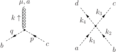
Figure 5: Momentum routing for the tree level ghost-gluon and four-ghost vertices.

Ghost and gluon propagators:

The full ghost and gluon propagators in coordinate space are defined to be

$$\langle c^{a}(x)\bar{c}^{b}(y)\rangle = \frac{\delta W}{\delta\sigma^{b}(y)\delta\bar{\sigma}^{a}(x)}=D_{G}^{ab}(x-y)$$ (81)

$$\langle A_{\mu}^{a}(x)A_{\nu}^{b}(y)\rangle = \frac{\delta W}{\delta J_{\nu}^{b}(y)\delta J_{\nu}^{a}(x)}=D_{\mu\nu}^{ab}(x-y).$$ (82)

The bare propagators in coordinate space can be easily derived from the quadratic part of the action,

$$S_{quad}=\int d^{4}x^{\prime}\left\{\frac{1}{2}A_{\mu}^{a}\left(-\partial^{2}\delta_{\mu\nu}+\left(1-\frac{1}{\lambda}\right)\partial_{\mu}\partial_{\nu}\right)A_{\nu}^{a}+\bar{c}^{a}\partial^{2}c^{a}\right\}$$ (84)

and are given by

$$\left[D_{G}^{(0)ab}(x-y)\right]^{-1} = \frac{\delta^{2}S_{{quad}}}{\delta\bar{c}^{a}(x)c^{b}(y)}\hskip 8.53581pt=\delta^{ab}\partial^{2}\delta(x-y)\,,$$ (85)

$$\left[D_{\mu\nu}^{(0)ab}(x-y)\right]^{-1} = \frac{\delta^{2}S_{{quad}}}{\delta A_{\mu}^{a}(x)A_{\nu}^{b}(y)}=\delta^{ab}\left(-\partial^{2}\delta_{\mu\nu}+\left(1-\frac{1}{\lambda}\right)\partial_{\mu}\partial_{\nu}\right)\,\delta(x-y)\,,\hskip 28.45274pt$$ (86)

with the gauge parameter $\lambda$. After Fourier transformation one obtains the corresponding expressions in momentum space:

$$\left[D_{G}^{(0)ab}(p)\right]^{-1} = -\delta^{ab}p^{2}$$ (87)

$$\left[D_{\mu\nu}^{(0)ab}(p)\right]^{-1} = \delta^{ab}\left(\delta_{\mu\nu}-\left(1-\frac{1}{\lambda}\right)\frac{p_{\mu}p_{\nu}}{p^{2}}\right)p^{2}.$$ (88)

Ghost-gluon vertex:

From the ghost gluon part of the action

$$S_{ghgl}=\int d^{4}x^{\prime}\left\{-i\left(1-\frac{\alpha}{2}\right)gf^{abc}\left(\partial^{\mu}\bar{c}\right)A^{c}_{\mu}c^{b}+i\frac{\alpha}{2}gf^{abc}\bar{c^{a}}A_{\mu}^{c}\partial^{\mu}c^{b}\right\}$$ (89)

the tree level ghost gluon vertex $\Gamma_{\mu}^{abc}$ is easily derived:

$$\Gamma_{\mu}^{(0)abc}(x,y,z) = \frac{\delta^{3}S_{ghgl}}{\delta A_{\mu}^{a}(x)\delta\bar{c}^{b}(y)\delta c^{c}(z)}$$

$$= -gf^{abc}\left[i\left(1-\frac{\alpha}{2}\right)\left(\partial_{\mu}^{z}\delta^{4}(z-y)\right)\delta^{4}(z-x)+i\frac{\alpha}{2}\partial_{\mu}^{z}\left(\delta^{4}(z-y)\delta^{4}(z-x)\right)\right].$$

Using the momentum conventions of Fig. 5 the Fourier transformed bare ghost-gluon vertex reads

$$\Gamma_{\mu}^{(0)abc}(k,p,q) = \int d^{4}[xyz]\,\Gamma_{\mu}^{abc}(x,y,z)\,e^{i(k\cdot x+q\cdot y-p\cdot z)}$$ (91)

$$= gf^{abc}\,(2\pi)^{4}\,\delta^{4}(k+q-p)\,\left[\left(1-\frac{\alpha}{2}\right)q_{\mu}+\frac{\alpha}{2}p_{\mu}\right]\,,$$

where the abbreviation $d^{4}x\,d^{4}y\,d^{4}z=:d^{4}[xyz]$ has been introduced. Note the symmetry of the vertex in the ghost momenta $p_{\mu}$ and $q_{\mu}$ if $\alpha=1$. For convenience we define a reduced vertex function $\Gamma_{\mu}^{(0)}(p,q)$ by

$$\Gamma_{\mu}^{(0)abc}(k,p,q) = gf^{abc}(2\pi)^{4}\delta^{4}(k+q-p)\Gamma_{\mu}^{(0)}(p,q)$$

$$\Gamma_{\mu}^{(0)}(p,q) = \left[\left(1-\frac{\alpha}{2}\right)q_{\mu}+\frac{\alpha}{2}p_{\mu}\right].$$ (92)

The full one particle irreducible ghost gluon vertex in coordinate space is given by

$$\Gamma_{\mu}^{abc}(x,y,z)=\frac{\delta\Gamma}{\delta J^{a}_{\mu}(x)\delta\bar{c}^{b}(y)\delta{c}^{c}(z)}.$$ (93)

Four-ghost vertex:

The four-ghost vertex $\Gamma_{4g}^{abcd}$ is derived from the four ghost part of the action

$$S_{4gh}=\int d^{4}x^{\prime}\left\{\frac{\alpha}{2}\left(1-\frac{\alpha}{2}\right)\frac{\lambda}{2}g^{2}f^{ace}f^{bde}\bar{c}^{a}\bar{c}^{b}c^{c}c^{d}\right\}$$ (94)

which leads to

$$\Gamma_{4g}^{(0)abcd}(x,y,z,w) = \frac{\delta^{4}S_{4gh}}{\delta\bar{c}^{a}(x)\delta\bar{c}^{b}(y)\delta c^{c}(z)\delta c^{d}(w)}$$ (95)

$$= \frac{\alpha}{2}\left(1-\frac{\alpha}{2}\right)\lambda g^{2}f^{abe}f^{cde}\delta^{4}(x-y)\delta^{4}(y-z)\delta^{4}(z-w).$$

Again using the momentum conventions of figure (5) one obtains for the Fourier-transformed bare four-ghost vertex

$$\Gamma_{4g}^{(0)abcd}(k_{1},k_{2},k_{3},k_{4}) = \frac{\delta^{4}S_{4gh}}{\delta\bar{c}^{a}(x)\delta\bar{c}^{b}(y)\delta c^{c}(z)\delta c^{d}(w)}$$ (96)

$$= \frac{\alpha}{2}\left(1-\frac{\alpha}{2}\right)\lambda g^{2}f^{abe}f^{cde}(2\pi)^{4}\delta^{4}(k_{1}+k_{2}-k_{3}-k_{4}).$$

We define a reduced vertex function $\Gamma_{4g}^{(0)}$ by

$$\Gamma_{4g}^{(0)abcd}(k_{1},k_{2},k_{3},k_{4}) = g^{2}f^{abe}f^{cde}(2\pi)^{4}\delta^{4}(k_{1}+k_{2}-k_{3}-k_{4})\Gamma_{4g}^{(0)}$$

$$\Gamma_{4g}^{(0)} = \frac{\alpha}{2}\left(1-\frac{\alpha}{2}\right)\lambda.$$ (97)

The full four-ghost vertex in coordinate space is formally given by

$$\Gamma^{abcd}(x,y,z)=\frac{\delta\Gamma}{\delta\bar{c}^{a}(x)\delta\bar{c}^{b}(y)\delta{c}^{c}(z)\delta{c}^{d}(y)}.$$ (98)

Decomposition of connected ghost-gluon Green’s function:

With the help of the matrix relation

$$\frac{\delta\chi^{-1}}{\delta\phi}=-\chi^{-1}\frac{\delta\chi}{\delta\phi}\chi^{-1},$$ (99)

and the identity

$$\delta(y-x)\delta^{ab}=\int d^{4}z\frac{\delta\bar{\sigma}^{b}(y)}{\delta\bar{c}^{d}(z)}\frac{\delta\bar{c}^{d}(z)}{\delta\bar{\sigma}^{a}(x)} = \int d^{4}z\frac{\delta^{2}\Gamma}{\delta\bar{c}^{d}(z)\delta c^{b}(y)}\frac{\delta^{2}W}{\delta\bar{\sigma}^{a}(x)\delta\sigma^{d}(z)}\,,$$ (100)

we decompose the connected ghost-gluon correlation function, $\langle A^{a}_{\mu}(x)\bar{c}^{b}(y)c^{c}(z)\rangle$, in the following way:

$$\langle A^{a}_{\mu}(x)\bar{c}^{b}(y)c^{c}(z)\rangle = \frac{\delta^{3}W}{\delta J^{a}_{\mu}(x)\delta\bar{\sigma}^{b}(y)\delta{\sigma}^{c}(z)}$$ (101)

$$=\frac{\delta}{\delta J^{a}_{\mu}(x)}\left[\frac{\delta^{2}\Gamma}{\delta\bar{c}^{b}(y)\delta{c}^{c}(z)}\right]^{-1}$$

$$=\int d^{4}u_{1}\frac{\delta A^{d}_{\nu}(u_{1})}{\delta J^{a}_{\mu}(x)}\frac{\delta}{\delta A^{d}_{\nu}(u_{1})}\left[\frac{\delta^{2}\Gamma}{\delta\bar{c}^{b}(y)\delta{c}^{c}(z)}\right]^{-1}$$

$$=\int d^{4}[u_{1}u_{2}u_{3}]\frac{\delta^{2}W}{\delta J^{a}_{\mu}(x)\delta J^{d}_{\nu}(u_{1})}\>\frac{\delta^{2}W}{\delta\bar{\sigma}^{b}(y)\delta{\sigma}^{e}(u_{2})}\>\frac{\delta^{3}\Gamma}{\delta A^{d}_{\nu}(u_{1})\delta\bar{c}^{e}(u_{2})\delta{c}^{f}(u_{3})}\>\frac{\delta^{2}W}{\delta\bar{\sigma}^{f}(u_{3})\delta{\sigma}^{c}(z)}$$

$$=\int d^{4}[u_{1}u_{2}u_{3}]D_{\mu\nu}^{ad}(x-u_{1})D_{G}^{eb}(u_{2}-y)\Gamma^{def}_{\nu}(u_{1},u_{2},u_{3})D_{G}^{cf}(u_{3}-z).$$

Here we used the abbreviation $d^{4}[u_{1}u_{2}u_{3}]:=d^{4}u_{1}\,d^{4}u_{2}\,d^{4}u_{3}$ and the definitions of the gluon propagator $D_{\mu\nu}$, the ghost propagator $D_{G}$ and the ghost-gluon vertex $\Gamma_{\nu}$ given in previous subsections.

Decomposition of connected four ghost Green’s function:

Furthermore we need the decomposition of the four-ghost correlation function into one-particle irreducible parts. We start at a stage where the sources are still present and set them to zero at the end of the derivation. We first give the decomposition of the connected ghost-antighost-ghost three-point function

$$\langle\bar{c}^{b}(y){c}^{c}(z)\bar{c}^{d}(w)\rangle = \frac{\delta^{3}W}{\delta\bar{\sigma}^{b}(y)\delta\sigma^{c}(z)\delta\bar{\sigma}^{d}(w)}$$

$$=\frac{\delta}{\delta\bar{\sigma}^{b}(y)}\left[\frac{\delta^{2}\Gamma}{\delta\sigma^{c}(z)\delta\bar{\sigma}^{d}(w)}\right]^{-1}$$

$$=\int d^{4}u_{1}\frac{\delta A^{e}_{\nu}(u_{1})}{\delta\bar{\sigma}^{b}(y)}\frac{\delta}{\delta A^{e}_{\nu}(u_{1})}\left[\frac{\delta^{2}\Gamma}{\delta\sigma^{c}(z)\delta\bar{\sigma}^{d}(w)}\right]^{-1}$$

$$=\int d^{4}[u_{1}u_{2}u_{3}]\frac{\delta^{2}W}{\delta\bar{\sigma}^{b}(y)\delta J^{e}_{\nu}(u_{1})}\>\frac{\delta^{2}W}{\delta\sigma^{c}(z)\delta\bar{\sigma}^{f}(u_{2})}\>\frac{\delta^{3}\Gamma}{\delta A^{e}_{\nu}(u_{1})\delta{c}^{f}(u_{2})\delta\bar{c}^{g}(u_{3})}\>\frac{\delta^{2}W}{\delta\sigma^{g}(u_{3})\delta\bar{\sigma}^{d}(w)}\,.$$

Then we decompose the connected four-ghost Green’s function:

$$\langle{c}^{a}(x)\bar{c}^{b}(y){c}^{c}(z)\bar{c}^{d}(w)\rangle = \frac{\delta^{4}W}{\delta\sigma^{a}(x)\delta\bar{\sigma}^{b}(y)\delta\sigma^{c}(z)\delta\bar{\sigma}^{d}(w)}$$ (103)

$$= \frac{\delta}{\delta\sigma^{a}(x)}\int d^{4}[u_{1}u_{2}u_{3}]\frac{\delta^{2}W}{\delta\bar{\sigma}^{b}(y)\delta J^{e}_{\mu}(u_{1})}\>\frac{\delta^{2}W}{\delta\sigma^{c}(z)\delta\bar{\sigma}^{f}(u_{2})}$$

$$\hskip 42.67912pt\times\frac{\delta^{3}\Gamma}{\delta A^{e}_{\mu}(u_{1})\delta{c}^{f}(u_{2})\delta\bar{c}^{g}(u_{3})}\>\frac{\delta^{2}W}{\delta\sigma^{g}(u_{3})\delta\bar{\sigma}^{d}(w)}.\hskip 28.45274pt$$

Carrying out the remaining derivative gives four terms. The two terms where the derivative acts on the second and on the last propagator vanish, because the term $\frac{\delta W}{\delta\bar{\sigma}^{b}(y)\delta J^{e}_{\nu}(u_{1})}$ vanishes when the sources are set to zero. The contribution where the derivative acts on the first propagator can be treated using eq. (101). In the expression with the derivative acting on the vertex we use

$$-\frac{\delta^{2}W}{\delta\bar{\sigma}^{b}(y)\delta J^{e}_{\mu}(u_{1})}\frac{\delta^{4}\Gamma}{\delta\sigma^{a}(x)\delta A^{e}_{\mu}(u_{1})\delta{c}^{f}(u_{2})\delta\bar{c}^{g}(u_{3})} = \frac{\delta^{4}\Gamma}{\delta\sigma^{a}(x)\delta\bar{\sigma}^{b}(y)\delta{c}^{f}(u_{2})\delta\bar{c}^{g}(u_{3})}$$

$$=\int d^{4}u_{4}\frac{\delta^{2}W}{\delta\sigma^{a}(x)\bar{\sigma}^{e}(u_{4})}\>\>\frac{\delta^{4}\Gamma}{\delta c^{e}(u_{4})\delta\bar{\sigma}^{b}(y)\delta{c}^{f}(u_{2})\delta\bar{c}^{g}(u_{3})}$$

$$=\int d^{4}[u_{4}u_{5}]\frac{\delta^{2}W}{\delta\sigma^{a}(x)\bar{\sigma}^{e}(u_{4})}\>\>\frac{\delta^{2}W}{\delta\bar{\sigma}^{b}(y)\delta{\sigma}^{h}(u_{5})}\>\>\frac{\delta^{4}\Gamma}{\delta c^{e}(u_{4})\delta\bar{c}^{h}(u_{5})\delta{c}^{f}(u_{2})\delta\bar{c}^{g}(u_{3})}$$

$$=-\int d^{4}[u_{4}u_{5}]\frac{\delta^{2}W}{\delta\sigma^{a}(x)\bar{\sigma}^{e}(u_{4})}\>\>\frac{\delta^{2}W}{\delta{\sigma}^{h}(u_{5})\delta\bar{\sigma}^{b}(y)}\>\>\frac{\delta^{4}\Gamma}{\delta\bar{c}^{g}(u_{3})\delta\bar{c}^{h}(u_{5})\delta c^{e}(u_{4})\delta{c}^{f}(u_{2})}.$$

Collecting all this together we arrive at

$$\langle{c}^{a}(x)\bar{c}^{b}(y){c}^{c}(z)\bar{c}^{d}(w)\rangle = \int d^{4}[u_{1}u_{2}u_{3}u_{4}u_{5}u_{6}]\left\{\frac{\delta^{2}W}{\delta J^{e}_{\mu}(u_{1})\delta J^{f}_{\nu}(u_{4})}\>\>\frac{\delta^{2}W}{\delta\sigma^{a}(x)\delta\bar{\sigma}^{g}(u_{5})}\right.$$ (105)

$$\hskip 28.45274pt\times\frac{\delta^{3}\Gamma}{\delta A^{f}_{\nu}(u_{4})\delta{c}^{g}(u_{5})\delta\bar{c}^{h}(u_{6})}\>\>\frac{\delta^{2}W}{\delta\sigma^{h}(u_{6})\delta\bar{\sigma}^{b}(y)}\>\>\frac{\delta^{2}W}{\delta\sigma^{c}(z)\delta\bar{\sigma}^{i}(u_{2})}$$

$$\hskip 28.45274pt\left.\times\frac{\delta^{3}\Gamma}{\delta A^{e}_{\mu}(u_{1})\delta{c}^{i}(u_{2})\delta\bar{c}^{j}(u_{3})}\>\>\frac{\delta^{2}W}{\delta\sigma^{j}(u_{3})\delta\bar{\sigma}^{d}(w)}\right\}$$

$$- \int d^{4}[u_{1}u_{2}u_{3}u_{4}u_{5}]\left\{\frac{\delta^{2}W}{\delta\sigma^{a}(x)\bar{\sigma}^{e}(u_{4})}\>\>\frac{\delta^{2}W}{\delta{\sigma}^{h}(u_{5})\delta\bar{\sigma}^{b}(y)}\right.$$

$$\hskip 28.45274pt\times\frac{\delta^{2}W}{\delta\sigma^{c}(z)\delta\bar{\sigma}^{f}(u_{2})}\>\>\frac{\delta^{4}\Gamma}{\delta\bar{c}^{g}(u_{3})\delta\bar{c}^{h}(u_{5})\delta c^{e}(u_{4})\delta{c}^{f}(u_{2})}$$

$$\hskip 28.45274pt\times\left.\frac{\delta^{2}W}{\delta\sigma^{g}(u_{3})\delta\bar{\sigma}^{d}(w)}\right\}.$$

Interchanging some Grassmann fields in the correlations and using the definitions for the propagators and vertices given in the previous subsections we arrive at

$$\langle\bar{c}^{b}(y)\bar{c}^{d}(w){c}^{a}(x){c}^{c}(z)\rangle = \int d^{4}[u_{1}u_{2}u_{3}u_{4}u_{5}u_{6}]\left\{D_{\mu\nu}^{ef}(u_{1}-u_{4})\,D_{G}^{ag}(x-u_{5})\right.$$ (106)

$$\hskip 28.45274pt\times\Gamma^{fhg}_{\nu}(u_{4},u_{6},u_{5})D_{G}^{hb}(u_{6}-y)\,D_{G}^{ci}(z-u_{2})$$

$$\hskip 28.45274pt\left.\times\Gamma^{eji}_{\mu}(u_{1},u_{3},u_{2})\,D_{G}^{jd}(u_{3}-w)\right\}$$

$$+ \int d^{4}[u_{1}u_{2}u_{3}u_{4}u_{5}]\left\{D_{G}^{ae}(x-u_{4})\,D_{G}^{hb}(u_{5}-y)\right.$$

$$\hskip 28.45274pt\left.\times D_{G}^{cf}(z-u_{2})\,\Gamma_{4gh}^{hgef}(u_{5},u_{3},u_{4},u_{2})\,D_{G}^{gd}(u_{3}-w)\right\},\hskip 28.45274pt$$

which is the decomposition of the four-ghost correlation used in appendix A.

Appendix C Appendix C: Tensor integrals

The explicit expression for the scalar bubble integral $I$, defined in eq. (107), can be easily evaluated in Euclidean space-time using the Feynman-parameterisation. With the squared momenta $x=p^{2}$, $y=q^{2}$ and $z=(p-q)^{2}$ the result is given by

$$I(a,b,p) := \int d^{4}q\frac{1}{y^{a}z^{b}}$$ (107)

$$= \pi^{2}\,x^{2-a-b}\,\frac{\Gamma(2-a)\,\Gamma(2-b)\,\Gamma(a+b-2)}{\Gamma(a)\,\Gamma(b)\,\Gamma(4-a-b)}\,.$$ (108)

The corresponding tensor integrals can be reduced to scalar integrals by extracting combinations of momenta $p_{\mu}$ and the symmetric tensor $\delta_{\mu\nu}$ according to the symmetry properties of the integrand:

$$J_{\mu}(a,b,p) := \int d^{4}q\frac{q_{\mu}}{y^{a}z^{b}}\hskip 19.91684pt=J_{1}(a,b,p)\,\,p_{\mu}\,,$$ (109)

$$K_{\mu\nu}(a,b,p) := \int d^{4}q\frac{q_{\mu}q_{\nu}}{y^{a}z^{b}}\hskip 17.07182pt\,=K_{1}(a,b,p)\,\,p_{\mu}p_{\nu}+K_{2}(a,b,p)\,\,x\,\delta_{\mu\nu}\,,$$ (110)

$$L_{\mu\nu\rho}(a,b,p) := \int d^{4}q\frac{q_{\mu}q_{\nu}q_{\rho}}{y^{a}z^{b}}\hskip 8.5359pt\,=L_{1}(a,b,p)\,\,p_{\mu}p_{\nu}p_{\rho}$$ (111)

$$\hskip 76.82234pt\,+\,L_{2}(a,b,p)\,\,x\,\left(p_{\mu}\,\delta_{\nu\rho}+p_{\nu}\,\delta_{\rho\mu}+p_{\rho}\,\delta_{\mu\nu}\right)\,,$$

$$M_{\mu\nu\rho\sigma}(a,b,p) := \int d^{4}q\frac{q_{\mu}q_{\nu}q_{\rho}q_{\sigma}}{y^{a}z^{b}}=M_{1}(a,b,p)\,\,p_{\mu}p_{\nu}p_{\rho}p_{\sigma}$$ (112)

$$\hskip 79.6678pt+\,M_{2}(a,b,p)\,\,x\,\left(\delta_{\mu\nu}\,p_{\rho}p_{\sigma}+\delta_{\mu\rho}\,p_{\nu}p_{\sigma}+\delta_{\mu\sigma}\,p_{\rho}p_{\mu}+\right.$$

$$\hskip 159.3356pt\left.\,\delta_{\nu\rho}\,p_{\mu}p_{\sigma}+\delta_{\nu\sigma}\,p_{\rho}p_{\mu}+\delta_{\rho\sigma}\,p_{\mu}p_{\nu}\right)$$

$$\hskip 79.6678pt+\,M_{3}(a,b,p)\,\,x^{2}\,\left(\delta_{\mu\nu}\,\delta_{\rho\sigma}+\delta_{\mu\rho}\,\delta_{\nu\sigma}+\delta_{\mu\sigma}\,\delta_{\rho\nu}\right)\,.\hskip 28.45274pt$$

The scalar integrals in these expressions are calculated by contracting them with appropriate tensors, writing all scalar products in terms of squared momenta $x,y$ and $z$ and applying eq. (108). One arrives at

$$J_{1} = \pi^{2}\frac{\Gamma(3-a)\,\Gamma(2-b)\,\Gamma(a+b-2)}{\Gamma(a)\,\Gamma(b)\,\Gamma(5-a-b)}\,x^{2-a-b}\,,$$ (113)

$$K_{1} = \pi^{2}\frac{\Gamma(4-a)\,\Gamma(2-b)\,\Gamma(a+b-2)}{\Gamma(a)\,\Gamma(b)\,\Gamma(6-a-b)}\,x^{2-a-b}\,,$$ (114)

$$K_{2} = \pi^{2}\frac{\Gamma(3-a)\,\Gamma(3-b)\,\Gamma(a+b-2)}{\Gamma(a)\,\Gamma(b)\,\Gamma(6-a-b)}\,\frac{1}{2(-3+a+b)}\,x^{2-a-b}\,,$$ (115)

$$L_{1} = \pi^{2}\frac{\Gamma(5-a)\,\Gamma(2-b)\,\Gamma(a+b-2)}{\Gamma(a)\,\Gamma(b)\,\Gamma(7-a-b)}\,x^{2-a-b}\,,$$ (116)

$$L_{2} = \pi^{2}\frac{\Gamma(4-a)\,\Gamma(3-b)\,\Gamma(a+b-2)}{\Gamma(a)\,\Gamma(b)\,\Gamma(7-a-b)}\,\frac{1}{2(-3+a+b)}\,x^{2-a-b}\,,$$ (117)

$$M_{1} = \pi^{2}\frac{\Gamma(6-a)\,\Gamma(2-b)\,\Gamma(a+b-2)}{\Gamma(a)\,\Gamma(b)\,\Gamma(8-a-b)}\,x^{2-a-b}\,,$$ (118)

$$M_{2} = \pi^{2}\frac{\Gamma(5-a)\,\Gamma(3-b)\,\Gamma(a+b-2)}{\Gamma(a)\,\Gamma(b)\,\Gamma(8-a-b)}\,\frac{1}{2(-3+a+b)}\,x^{2-a-b}\,,$$ (119)

$$M_{3} = \pi^{2}\frac{\Gamma(4-a)\,\Gamma(4-b)\,\Gamma(a+b-2)}{\Gamma(a)\,\Gamma(b)\,\Gamma(8-a-b)}\,\frac{1}{4(-3+a+b)(-4+a+b)}\,x^{2-a-b}\,.\hskip 28.45274pt$$ (120)

Appendix D Appendix D: Expressions for some diagrams in bare vertex approximation

In this appendix we give explicitly the expressions for some diagrams needed for our investigation in the main body of the paper. All algebraic manipulations have been done using the program FORM Form . Our ansätze for the small momentum behaviour of the ghost dressing function $G$, the transversal gluon dressing function $Z$ and the longitudinal gluon dressing function $L$ are the power laws

$$G(x)=Bx^{\beta},\>\>\>\>Z(x)=Ax^{\sigma},\>\>\>\>L(x)=Cx^{\rho},$$ (121)

where we have used the abbreviation $x=p^{2}$.

We first evaluate the sunset diagram in the ghost equation given diagrammatically in Fig. 6.

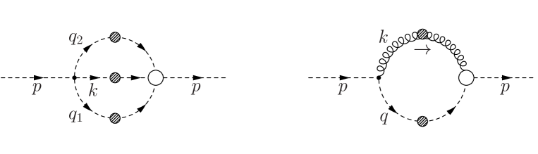
Figure 6: Momentum routing for the sunset and for the dressing diagram in the ghost equation.

With the bare four-ghost vertex given in eq. (97) and the abbreviations for the squared momenta $x=p^{2}$, $y_{1}=(q_{1})^{2}$, $y_{2}=(q_{2})^{2}$, $z_{1}=(p-q_{1})^{2}$ and $z_{2}=(p-q_{1}-q_{2})^{2}$ the sunset diagram reads

$$U^{sun}=\frac{N_{c}^{2}\,g^{4}\,\tilde{Z}_{4}}{2\,(2\pi)^{8}}\left(\frac{\alpha}{2}\left(1-\frac{\alpha}{2}\right)\lambda\right)^{2}\int d^{4}q_{1}\,\frac{B\,(y_{1})^{\beta}}{x\,y_{1}}\,\int d^{4}q_{2}\,\frac{B^{2}\,(y_{2})^{\beta}\,(z_{2})^{\beta}}{y_{2}\,z_{2}}.$$ (122)

The factor $1/x$ in the first integral stems from the left hand side of the ghost equation. We now integrate the inner loop with the help of formula (108) and obtain

$$U^{sun}=\frac{N_{c}^{2}\,g^{4}\,\tilde{Z}_{4}\,B^{3}}{512\,\pi^{6}}\left(\frac{\alpha}{2}\left(1-\frac{\alpha}{2}\right)\lambda\right)^{2}\frac{\Gamma^{2}(1+\beta)\,\Gamma(-2\beta)}{\Gamma^{2}(1-\beta)\,\Gamma(2+2\beta)}\,\int d^{4}q_{1}\,\frac{(y_{1})^{\beta}}{x\,y_{1}}\,(z_{1})^{2\beta}\,,$$ (123)

where $z_{1}$ is the total squared momentum flowing through the integrated loop. The second integration is done in the same way. We arrive at

$$U^{sun} = x^{3\beta}\,\frac{N_{c}^{2}\,g^{4}\,\tilde{Z}_{4}\,B^{3}}{512\,\pi^{4}}\left(\frac{\alpha}{2}\left(1-\frac{\alpha}{2}\right)\lambda\right)^{2}\frac{\Gamma^{3}(1+\beta)\,\Gamma(-3\beta-1)}{\Gamma^{3}(1-\beta)\,\Gamma(3+3\beta)}$$ (124)

$$:= x^{3\beta}(U^{\prime})^{sun}\,.$$

As each integration step eats up the two squared momenta in the denominators of the integral kernels only powers of $x$ to the anomalous dimensions of the dressing functions in the loop (here $3\beta$ from three ghost propagators) survive. This mechanism works in the same way for all diagrams and explains the pattern in the eqs. (41), (42) and (43) in the main body of the paper.

Next we evaluate the two contributions in the gluon equation needed for the argument below eq. (46). The explicit expressions for the kernels of two-loop gluon diagrams are rather lengthy but the calculation is done along the same lines as in the ghost sunset diagram above. Therefore we just give the final results:

$$V^{squint}_{TTTT} = x^{4\sigma}\,\frac{-27\,g^{4}\,N_{c}^{2}\,Z_{4}\,A^{4}}{4096\,\pi^{4}}\,\frac{\Gamma(-1-4\sigma)\>\Gamma(1/2-\sigma)\>\Gamma(3\sigma)\>\Gamma^{2}(1+\sigma)}{\Gamma(4-3\sigma)\>\Gamma^{2}(2-\sigma)\>\Gamma(3/2-\sigma)\>\Gamma(4+4\sigma)}\times$$ (125)

$$2^{-4\sigma}\>(-1+3\sigma)\>(10+\sigma-66\sigma^{2}+63\sigma^{3})\>(5+43\sigma+47\sigma^{2})$$

$$:= x^{4\sigma}\,(V^{\prime})^{squint}_{TTTT}\,,$$

$$W^{sun}_{LLL} = x^{3\delta}\,\frac{g^{4}\,N_{c}^{2}\,Z_{4}\,C^{3}}{1536\,\pi^{4}}\,\frac{1}{(1+3\delta)}\frac{\Gamma^{3}(1+\delta)\>\Gamma(1-3\delta)}{\Gamma^{3}(2-\delta)\>\Gamma(3+3\delta)}\>\>\lambda^{3}$$ (126)

$$:= x^{3\delta}\,(W^{\prime})^{sun}_{LLL}\,.$$

Finally we calculate that part in the dressing diagram of the ghost equation which contains the longitudinal part of the gluon propagator for the special case $\alpha=0,2$. These are the linear covariant gauges where $L(x)=1$ by virtue of the Slavnov-Taylor identity. Replacing dressed vertices with bare ones, however, violates this identity. We therefore start with the general expression, $L(x)=Cx^{\rho}$ and investigate whether the limit $\rho\rightarrow 0$ can be performed consistently. With the momentum assignments $x=p^{2}$, $y=q^{2}$ and $z=k^{2}=(p-q)^{2}$ the longitudinal part of the diagram is given by

$$U^{dress}_{L} = -\frac{N_{c}\,g^{2}\,\tilde{Z}_{1}\,\lambda}{(2\pi)^{4}}\int d^{4}q\,q_{\mu}\frac{k_{\mu}k_{\nu}}{z^{2}}p_{\nu}\frac{B\,y^{\beta}\,C\,z^{\rho}}{x\,y}$$

$$= -\frac{N_{c}\,g^{2}\,\tilde{Z}_{1}\,\lambda\,B\,C}{(2\pi)^{4}}\int d^{4}q\left\{p_{\mu}\frac{q_{\mu}}{y^{1-\beta}z^{2-\rho}}-\frac{p_{\mu}p_{\nu}}{x}\frac{q_{\nu}q_{\mu}}{y^{1-\beta}z^{2-\rho}}-\frac{1}{y^{-\beta}z^{2-\rho}}+\frac{p_{\mu}}{x}\frac{q_{\mu}}{y^{-\beta}z^{2-\rho}}\right\}$$

where again the extra factor $1/x$ stems from the left hand side of the ghost DSE. At this stage of the calculation it is not clear whether there are infrared singularities in the limit $\rho\rightarrow 0$. We employ the tensor integrals given in appendix C, use $x\Gamma(x)=\Gamma(1+x)$ and obtain

$$U^{dress}_{L} = -\frac{N_{c}\,g^{2}\,\tilde{Z}_{1}\,\lambda\,B\,C}{16\pi^{2}}x^{\beta+\rho}\frac{\Gamma(2+\beta)\Gamma(\rho)\Gamma(-\beta-\rho)}{\Gamma(-\beta)\Gamma(2-\rho)\Gamma(2+\rho+\beta)}\frac{\rho^{2}+\rho/2}{\beta(2+\beta+\rho)}\,.$$ (129)

In the limit $\rho\rightarrow 0$ this expression is infrared-finite, as $\lim_{\rho\rightarrow 0}\Gamma(\rho)\rho=1$. We then obtain

$$U^{dress}_{L} = -\frac{N_{c}\,g^{2}\,\tilde{Z}_{1}\,\lambda\,B\,C}{16\pi^{2}}x^{\beta}\frac{1}{2\beta(2+\beta)}\,.$$ (130)

References

• (1) D. Zwanziger, arXiv:hep-ph/0303028.
• (2) P. Maris and C. D. Roberts, arXiv:nucl-th/0301049.
C. D. Roberts and S. M. Schmidt, Prog. Part. Nucl. Phys. 45, S1 (2000) [arXiv:nucl-th/0005064].
• (3) R. Alkofer and L. von Smekal, Phys. Rept.  353, 281 (2001) [arXiv:hep-ph/0007355].
• (4) L. von Smekal, R. Alkofer and A. Hauck, Phys. Rev. Lett.  79, 3591 (1997)
[arXiv:hep-ph/9705242]; Annals Phys.  267, 1 (1998) [arXiv:hep-ph/9707327].
• (5) D. Atkinson and J. C. Bloch, Phys. Rev. D 58, 094036 (1998) [arXiv:hep-ph/9712459];
Mod. Phys. Lett. A13, 1055 (1998) [arXiv:hep-ph/9802239].
• (6) J. C. Bloch, arXiv:hep-ph/0303125.
• (7) D. Zwanziger, Phys. Rev. D 65, 094039 (2002) [arXiv:hep-th/0109224].
• (8) C. Lerche and L. von Smekal, Phys. Rev. D 65, 125006 (2002) [arXiv:hep-ph/0202194].
• (9) C. S. Fischer and R. Alkofer, Phys. Lett. B536, 177 (2002) [arXiv:hep-ph/0202202]; C. S. Fischer, R. Alkofer and H. Reinhardt, Phys. Rev. D 65, 094008 (2002) [arXiv:hep-ph/0202195]; R. Alkofer, C. S. Fischer and L. von Smekal, arXiv:hep-ph/0301107; arXiv:nucl-th/0301048.
• (10) F. D. Bonnet, P. O. Bowman, D. B. Leinweber and A. G. Williams, Phys. Rev. D 62, 051501 (2000) [arXiv:hep-lat/0002020].
• (11) F. D. Bonnet, P. O. Bowman, D. B. Leinweber, A. G. Williams and J. M. Zanotti, Phys. Rev. D 64, 034501 (2001) [arXiv:hep-lat/0101013].
• (12) K. Langfeld, H. Reinhardt and J. Gattnar, Nucl. Phys. B 621, 131 (2002) [arXiv:hep-ph/0107141]; arXiv:hep-lat/0110025.
• (13) H. Suman and K. Schilling, Phys. Lett. B 373 (1996) 314 [arXiv:hep-lat/9512003].
• (14) A. Cucchieri, Nucl. Phys. B 508 (1997) 353 [arXiv:hep-lat/9705005].
• (15) C. S. Fischer and R. Alkofer, Phys. Rev. D 67 (2003) 094020 [arXiv:hep-ph/0301094].
• (16) T. Kugo and I. Ojima, Prog. Theor. Phys. Suppl. 66, 1 (1979).
• (17) N. Nakanishi and I. Ojima, Covariant Operator Formalism of Gauge Theories and Quantum Gravity, World Scientific, 1990.
• (18) L. Baulieu and J. Thierry-Mieg, Nucl. Phys. B 197 (1982) 477; J. Thierry-Mieg, Nucl. Phys. B 261 (1985) 55.
• (19) D. Zwanziger, arXiv:hep-th/0206053.
• (20) A. P. Szczepaniak and E. S. Swanson, Phys. Rev. D 65, 025012 (2002) [arXiv:hep-ph/0107078];
C. Feuchter, K. Langfeld, L. Moyaerts and H. Reinhardt, to be published.
• (21) A. Cucchieri and D. Zwanziger, Nucl. Phys. Proc. Suppl.  106, 694 (2002) [arXiv:hep-lat/0110189]; A. Cucchieri, T. Mendes and D. Zwanziger, Nucl. Phys. Proc. Suppl.  106, 697 (2002) [arXiv:hep-lat/0110188]; A. Cucchieri and D. Zwanziger, Phys. Lett. B 524, 123 (2002) [arXiv:hep-lat/0012024]; A. Cucchieri and D. Zwanziger, Phys. Rev. D 65, 014001 (2002) [arXiv:hep-lat/0008026];
• (22) A. Cucchieri and D. Zwanziger, Phys. Rev. D 65, 014002 (2002) [arXiv:hep-th/0008248].
• (23) L. Baulieu and D. Zwanziger, Nucl. Phys. B 548, 527 (1999) [arXiv:hep-th/9807024].
• (24) D. Zwanziger, Phys. Rev. Lett.  90, 102001 (2003) [arXiv:hep-lat/0209105].
• (25) J. Greensite and S. Olejnik, arXiv:hep-lat/0302018.
• (26) A. P. Szczepaniak and E. S. Swanson, Phys. Rev. D 55, 3987 (1997) [arXiv:hep-ph/9611310]; A. P. Szczepaniak and P. Krupinski, arXiv:hep-ph/0204249.
• (27) R. Alkofer and P. A. Amundsen, Nucl. Phys. B 306, 305 (1988); K. Langfeld, R. Alkofer and P. A. Amundsen, Z. Phys. C 42, 159 (1989); R. Alkofer and P. A. Amundsen, Phys. Lett. B 187, 395 (1987);
• (28) M. J. Lavelle and M. Schaden, Phys. Lett. B 208, 297 (1988).
• (29) P. Boucaud, A. Le Yaouanc, J. P. Leroy, J. Micheli, O. Pene and J. Rodriguez-Quintero, Phys. Rev. D 63, 114003 (2001) [arXiv:hep-ph/0101302].
• (30) K. I. Kondo, Phys. Lett. B 514, 335 (2001) [arXiv:hep-th/0105299].
• (31) L. Stodolsky, P. van Baal and V. I. Zakharov, Phys. Lett. B 552, 214 (2003) [arXiv:hep-th/0210204].
• (32) D. Dudal, H. Verschelde, V. E. Lemes, M. S. Sarandy, S. P. Sorella and M. Picariello, arXiv:hep-th/0302168.
• (33) M. Schaden, arXiv:hep-th/9909011.
• (34) F. V. Gubarev, L. Stodolsky and V. I. Zakharov, Phys. Rev. Lett.  86, 2220 (2001) [arXiv:hep-ph/0010057].
• (35) D. Zwanziger, private communication.
• (36) P. van Baal, private communication.
• (37) B. M. Gripaios, arXiv:hep-th/0302015.
• (38) J. de Boer, K. Skenderis, P. van Nieuwenhuizen and A. Waldron, Phys. Lett. B 367, 175 (1996) [arXiv:hep-th/9510167].
• (39) R. E. Browne and J. A. Gracey, Phys. Lett. B 540, 68 (2002) [arXiv:hep-th/0206111]; J. A. Gracey, Phys. Lett. B 552, 101 (2003) [arXiv:hep-th/0211144].
• (40) J. A. Vermaseren, arXiv:math-ph/0010025.
• (41) P. Watson and R. Alkofer, Phys. Rev. Lett.  86, 5239 (2001) [arXiv:hep-ph/0102332]; R. Alkofer, L. von Smekal and P. Watson, Proceedings of the ECT* Collaboration Meeting on Dynamical Aspects of the QCD Phase Transition, Trento, Italy, March 12-15, 2001, arXiv:hep-ph/0105142.