A Dilatonic Deformation of $AdS_{5}$ and its Field Theory Dual

Dongsu Bak,$\!{}^{1}$ Michael Gutperle^2,3 and Shinji Hirano⁴

¹ Physics Department, University of Seoul, Seoul 130-743, Korea

² Department of Physics and Astronomy, UCLA, Los Angeles, CA, USA

³ ITP, Department of Physics, Stanford University, Stanford, CA, USA

⁴ Department of Physics, Technion, Israel Institute of Technology, Haifa 32000, Israel abcdefg

We find a nonsupersymmetric dilatonic deformation of $AdS_{5}$ geometry as an exact nonsingular solution of the type IIB supergravity. The dual gauge theory has a different Yang-Mills coupling in each of the two halves of the boundary spacetime divided by a codimension one defect. We discuss the geometry of our solution in detail, emphasizing the structure of the boundary, and also study the string configurations corresponding to Wilson loops. We also show that the background is stable under small scalar perturbations.

1 Introduction

The AdS/CFT duality [1, 2, 3] beautifully exemplified the idea of holography [4][5] in clarity and precision, more powerfully than any other examples of the gravity/field theory correspondence. Since then there has already been a large volume of applications of the AdS/CFT [6]. Yet there may still be novel interesting avenues to be unfolded and pursued in its application.

As an example, in this paper, we will consider a dilatonic deformation of $AdS_{5}$ space, i.e. an asymptotically $AdS_{5}$ space with a spatially varying dilaton, which is a non-supersymmetric, yet (classically) exact, solution of type IIB supergravity. In fact there exists a class of dilatonic deformations of $AdS_{5}$ space of this kind, where the dilaton varies not only spatially but also in time. A time-dependent solution might be interesting in its own right. We will give a short description of these solutions in the discussion. However we found that the solution displayed a naked singularity, and hence it is not clear whether they are viable solutions in string theory.

Unlike the time-dependent solution, the deformation we will discuss in this paper is regular everywhere, and breaks the isometry $SO(4,2)$ of $AdS_{5}$ space down to $SO(3,2)$. The spacetime is asymptotically $AdS_{5}$, and the dilaton approaches to a constant at the boundary. However the value of the constant dilaton differs in one-half of the boundary from the other, leaving a codimension one defect at their junction. Our dilatonic solution thus reveals two different “faces” at the boundary, which led us to a coinage the “Janusian” solution.

Being non-supersymmetric, our solution is potentially unstable. We will analyze and discuss the stability of scalar perturbations about the solution, a more complete analysis of the stability including other modes is left for future work. From the dual field theory viewpoint, we are turning on a marginal deformation by the operator ${\cal O}_{4}\sim\mbox{Tr}(F^{2})$ dual to the dilaton, but with different deformation parameters in different halves of the flat boundary spacetime. The deformation is marginal, so it preserves the dilation invariance, $SO(1,1)$. But it breaks a part of the Lorentz symmetry down to $SO(2,1)$ due to the jump of the deformation parameter at the codimension one defect. Hence the ($2+1$)-dimensional conformal invariance, $SO(3,2)$, is left unbroken.

Having the $SO(3,2)$ isometry unbroken and the codimension one defect at the boundary, our solution is quite reminiscent of that of [11], where an $AdS_{4}$ brane inside an $AdS_{5}$ space was considered and it was shown that gravity is locally localized on the $AdS_{4}$ brane. The dual gauge theory is a defect conformal field theory (dCFT), and in the context of the AdS/CFT, it has already been studied in [14, 15, 16, 17]. However our solution differs significantly from [11] in that we do not have a source $AdS_{4}$ brane at all. Further the detailed form of the gravity dual of dCFT has not been known thus far. Our solution, though nonsupersymmetric, provides a simple example of an explicit gravity dual of dCFT. We will make more comments on these points later.

The organization of our paper is as follows. In section 2, we will review a few different parameterizations of AdS space, and discuss their boundary structure in some detail. In section 3, we will present our dilatonic solution and discuss its properties. In section 4, we will then discuss the geometry of the solution, in particular, emphasizing the structure of the boundary. We also make a comment on a relation of our solution to that of [11]. In section 5, we will present the interpretation of our solution in terms of the dual $N=4$ SYM theory, and also study the Wilson loop in our deformation. In section 6, we will discuss the stability of our solution. We will end with a brief discussion of possible generalizations and a time dependent solution which can be obtained by a slight modification of our ansatz.

2 The coordinate systems

For later use, we will review a couple of different coordinate systems for the $AdS_{d}$ space. The $AdS_{d}$ space is defined by a hyperboloid in $R^{2,d-1}$

$$X_{0}^{2}+X_{d}^{2}-X_{1}^{2}-\cdots-X_{d-1}^{2}=1\ .$$ (1)

(I) The global coordinate

The global coordinate covers the entire region of the $AdS_{d}$ space. It is obtained by the following parameterization,

$$X_{0}={\cos\tau\over\cos\theta},\quad X_{d}={\sin\tau\over\cos\theta},\quad X_{i}=\tan\theta\,\,n_{i},\;\;i=1,\cdots,d-1\ ,$$ (2)

where $n_{i}$ is the unit vector in $R^{d-1}$. The metric on the global $AdS_{d}$ is then given by

$$ds^{2}_{AdS_{d}}={1\over\cos^{2}\theta}\big{(}-d\tau^{2}+d\theta^{2}+\sin^{2}\theta\,d\Omega_{d-2}^{2}\big{)}\ ,$$ (3)

with $\theta\in\left[0,{\pi\over 2}\right]$.

(II) The Poincaré patch

In the AdS/CFT, the Poincaré patch is the most convenient parameterization of AdS space. Parameterizing $X_{0}={1\over 2}\left(z+\left(1+\vec{x}^{2}-t^{2}\right)/z\right)$, $X_{d}=t/z$, $X_{i=1,\cdots,d-2}=x_{i}/z$, and $X_{d-1}={1\over 2}\left(z-\left(1-\vec{x}^{2}+t^{2}\right)/z\right)$, the metric takes the form

$$ds_{AdS_{d}}^{2}={1\over z^{2}}\left(-dt^{2}+d\vec{x}^{2}+dz^{2}\right)\ ,$$ (4)

where $\vec{x}=(x_{1},\cdots,x_{d-2})$ and $z\in[0,\infty]$.

(III) The $AdS_{d-1}$ slicing

One can slice the $AdS_{d}$ space by $AdS_{d-1}$ spaces, which corresponds to parameterizing $X_{d-1}=z$ and the rest, $X_{i=0,\cdots,d}$, by any coordinate system of the $AdS_{d-1}$ space of radius $\sqrt{1+z^{2}}$. Then the metric takes the following form

$$ds_{AdS_{d}}^{2}={dz^{2}\over 1+z^{2}}+(1+z^{2})ds^{2}_{AdS_{d-1}}\ .$$ (5)

Defining a new coordinate $\mu$ by $z=\tan\mu$, the metric is rewritten as

$$ds_{AdS_{d}}^{2}=f(\mu)\big{(}d\mu^{2}+ds^{2}_{AdS_{d-1}}\big{)}\ ,$$ (6)

where $f(\mu)=1/\cos^{2}\mu$. Since the range of $z$ is $z\in[-\infty,+\infty]$, that of $\mu$ is $\mu\in\left[-{\pi\over 2},{\pi\over 2}\right]$. This is the most useful coordinate system for our application.

The boundary geometry

The conformal boundary of the global AdS metric (3) is located at $\theta=\pi/2$ and has the shape of $R\times S^{3}$ where $R$ is the time direction, while that of the Poincaré patch (4) is at $z=0$ and of the shape $R\times R^{3}$. In the $AdS_{d-1}$ slicing (6), the appearance of the boundary is less trivial. For later use, we will elaborate this point in some detail.

First we take the global coordinate for the $AdS_{d-1}$ slice in (6). Then the metric can be written as

$$ds^{2}_{AdS_{d}}={1\over\cos^{2}\mu\cos^{2}\lambda}\big{(}-d\tau^{2}+\cos^{2}\lambda d\mu^{2}+d\lambda^{2}+\sin^{2}\lambda d\Omega_{d-3}^{2}\big{)}\ ,$$ (7)

with $\lambda\in\left[0,{\pi\over 2}\right]$. The constant time section of this metric is conformal to a half of $S^{d-1}$, since the range of $\mu$ is from $-{\pi\over 2}$ to ${\pi\over 2}$. If $\mu$ had ranged over $[-\pi,\pi]$, it would have been the full sphere. The boundary, $\mu=\pm\pi/2$, of this half sphere is exactly that of a spatial section of the global $AdS_{d}$, thus being $S^{d-2}$. In fact the boundary consists of two parts, one of which is at $\mu=-\pi/2$ and the other at $\mu=\pi/2$. These two parts are joined through a surface, $\lambda=\pi/2$, which is a codimension one space in the boundary. The $\mu=\pi/2$ (or $\mu=-\pi/2$ ) part is $H^{d-2}$, a half of $S^{d-2}$, thus over all the boundary makes up the full $S^{d-2}$. Later we will encounter the case where the range of $\mu$ becomes larger. But the structure of the conformal boundary remains to be the same $S^{d-2}$.

Next we take the Poincaré patch for the $AdS_{d-1}$ slice in (6). Then the metric takes the form

$$ds^{2}_{AdS_{d}}={1\over y^{2}\cos^{2}\mu}\big{(}-dt^{2}+d\vec{x}_{d-3}^{2}+dy^{2}+y^{2}d\mu^{2}\big{)}\ ,$$ (8)

with $y\in[0,\infty]$. One can easily see that, by the change of coordinate $x=y\sin\mu$ and $z=y\cos\mu$, the above metric turns into the conventional form of the Poincare patch AdS,

$$ds^{2}_{AdS_{d}}={1\over z^{2}}\big{(}-dt^{2}+d\vec{x}_{d-3}^{2}+dx^{2}+dz^{2}\big{)}\ .$$ (9)

Again the boundary consists of two parts, one of which is at $\mu=\pi/2$ and the other at $\mu=-\pi/2$. These two parts are joined through a codimension one surface, $y=0$, forming a $d-2$ dimensional flat Euclidean space, or $d-1$ dimensional Minkowski space when including the time. Even with a larger range of $\mu$, as we will see below in our application, the structure of the conformal boundary remains the same, on which the dual $N=4$ SYM theory is defined.

3 The ansatz and the Janusian solution

In the following we will consider a simple deformation of $AdS_{5}$ space, which is asymptotically $AdS_{5}$ and has a nontrivial dilaton profile. We make the ansatz,

$$ds^{2} = f(\mu)\left(d\mu^{2}+ds^{2}_{AdS_{4}}\right)+ds_{S^{5}}^{2}\ ,$$

$$\phi = \phi(\mu)\ ,$$ (10)

$$F_{5} = 2f(\mu)^{5\over 2}d\mu\wedge\omega_{AdS_{4}}+2\omega_{S^{5}}\ ,$$

where $\omega_{AdS_{4}}$ and $\omega_{S^{5}}$ are the unit volume forms on $AdS_{4}$ and $S^{5}$ respectively. Thus, in particular, the five sphere $S^{5}$ is intact, so is the $SO(6)$ R-symmetry. But the supersymmetry is completely broken.

The IIB supergravity equations of motion are given by

$$R_{\alpha\beta}-{1\over 2}\partial_{\alpha}\phi\partial_{\beta}\phi-{1\over 4}F^{2}_{\alpha\beta}=0\ ,$$

$$\partial_{\alpha}(\sqrt{g}g^{\alpha\beta}\partial_{\beta}\phi)=0\ ,$$ (11)

$$*F_{5}=F_{5}\ ,$$

together with the Bianchi identity $dF_{5}=0$. The equation of motion for the dilaton (in the Einstein frame) is easily solved, giving

$$\phi^{\prime}(\mu)={c_{0}\over f^{3\over 2}(\mu)}\ .$$ (12)

The Einstein equations give rise to

$$2f^{\prime}f^{\prime}-2ff^{\prime\prime} = -4f^{3}+{c_{0}^{2}\over 2}{1\over f}\ ,$$

$$12f^{2}+f^{\prime}f^{\prime}+2ff^{\prime\prime} = 16f^{3}\,.$$ (13)

It is easy to see that these equations are equivalent to the first order differential equation

$$f^{\prime}f^{\prime}=4f^{3}-4f^{2}+{c_{0}^{2}\over 6}{1\over f}\ ,$$ (14)

corresponding to the motion of a particle with zero energy in a potential given by minus the right hand side (r.h.s.) of (14).

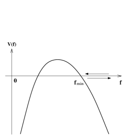
Figure 1: The dynamics corresponds to the particle motion under a potential with zero energy. We depict the shape of the potential here. We are interested in the trajectory in which the particle starts from infinity, reflected at $f_{min}$ and goes back to infinity.

Equation (14) can easily be integrated,

$$\mu=\int^{f}_{f_{min}}{d\tilde{f}\over 2\sqrt{\tilde{f}^{3}-\tilde{f}^{2}+{c_{0}^{2}\over 24}{1\over\tilde{f}}}}\ ,$$ (15)

where $f_{min}$ is the largest root of the denominator of the integrand. The function $f(\mu)$ is numerically solved in Figure 2.

Figure 2: $f(\mu)$ as a function of $\mu$ for values of $c_{0}=0.2,0.8,1.3$

Note that $c_{0}=0$ corresponds to a constant dilaton and (15) gives the $AdS_{4}$ slicing of (6). The integration region of $f$ is bounded by the (simple) zero of the r.h.s. of (14). Indeed the properties of the solution are determined by the behavior of the rational function

$$p(x)=x^{3}-x^{2}+{c_{0}^{2}\over 24x}\ ,$$ (16)

characterizing the potential, which has the following properties: For $c_{0}\in[0,{9\over 4\sqrt{2}}]$, it has two real zeros lying between 0 and 1. For $c_{cr}={9\over 4\sqrt{2}}$, two of the zeros coalesce and the function becomes

$$p(x)|_{c_{0}\to{9\over 4\sqrt{2}}}={1\over x}\left(x-{3\over 4}\right)^{2}\left(x^{2}+{1\over 2}x+{3\over 16}\right)\ .$$ (17)

For the critical $c_{cr}$ the integral (15) diverges logarithmically. For general $c_{0}\in[0,{9\over 4\sqrt{2}}]$ the rational function is of the form

$$p(x)={1\over x}(x-x_{1})(x-x_{2})((x-x_{3})^{2}+y_{3}^{2})\ ,$$ (18)

where $x_{1,2,3}$ and $y_{3}$ are functions of $c_{0}$.

As we increase $c_{0}$, the integrand in (15) is monotonically decreasing, but the integration over $f$ grows so quickly that it offsets and overwhelms the decreasing of the integrand. As shown in Figure 3 numerically, the total range of $\mu$ that is covered by the solution –the total time it takes for the particle to move from infinity and back– increases with increasing $c_{0}$.

Figure 3: The range of the coordinate $\mu$ as a functions of $c_{0}$, where $c_{0}$ varies from $0$ to $c_{crit}={9\over 4\sqrt{2}}$, $\mu_{0}$ starts from $\mu_{0}={\pi\over 2}$ and diverges at $c_{0}=c_{crit}$

Note that, since $f\to\infty$ at the edge of the range of $\mu$, the dilaton approaches to a constant in this limit. Hence for the noncritical range of $c_{0}$ –as long as $c_{0}$ is smaller than the critical value given below– the dilaton varies over a finite range and the string coupling can be made arbitrarily small;

$$\phi(\mu_{0})-\phi(-\mu_{0}) = \int_{-\mu_{0}}^{\mu_{0}}{c_{0}d\mu\over f^{3\over 2}(\mu)}$$ (19)

$$= 2\int_{f_{min}}^{\infty}{c_{0}df\over 2f^{3\over 2}\sqrt{f^{3}-f^{2}+{c_{0}^{2}\over 24}{1\over f}}}\ ,$$

where $\pm\mu_{0}$ is the maximum/minimum value of $\mu$, i.e $\mu\in[-\mu_{0},\mu_{0}]$. The dilaton equation (12) is numerically solved in Figure 4. Also the range of the dilaton, as $c_{0}$ varies, is shown numerically in Figure 5.

Figure 4: The dilaton $\phi$ as a functions of $\mu$, for values of $c_{0}=0.2,\;.8,\;1.3$

Figure 5: The range of the dilaton $\phi$ as a function of $c_{0}$, the range of the dilaton diverges at $c_{0}=c_{crit}$

Finally if $c_{0}$ exceeds $c_{cr}$, the zero energy motion of particle reaches the point $f=0$, where the geometry develops a naked singularity. We shall not consider this regime of upper critical solution below because we do not know how to deal with the singularity. It is an interesting question why such a drastic transition of geometry occurs depending on the strength $c_{0}$ of the dilaton perturbation at the boundary.

4 The geometry of the Janusian solution

In this section we would like to describe the geometry of our solution with an emphasis on the structure of the boundary. Since there is no change in the $S^{5}$ part, we only look at the $AdS_{5}$ directions. Adopting the global coordinate for the $AdS_{4}$ slice as in (7), the metric becomes

$$ds^{2}={f(\mu)\over\cos^{2}\lambda}\big{(}-d\tau^{2}+\cos^{2}\lambda d\mu^{2}+d\lambda^{2}+\sin^{2}\lambda d\Omega_{2}^{2}\big{)}\ .$$ (20)

The spatial section of the conformal metric, i.e. the metric inside the parenthesis is depicted in Figure 6. Only the surface of the globe parametrized by $\mu$ and $\lambda$ is relevant here. Each point on the surface represents $S^{2}$ and the boundary indicated by the bold lines is $S^{3}$. The boundary consists of two parts; one is at $\mu=-\mu_{0}$ and the other at $\mu=\mu_{0}$. These two halves of $S^{3}$ are joined through the north and south poles. The dilaton varies from one constant, $\phi_{0}^{-}=\phi(-\mu_{0})$, at one half of the boundary at $\mu=-\mu_{0}$, to another, $\phi_{0}^{+}=\phi(\mu_{0})$, at the other half of the boundary at $\mu=\mu_{0}$, running through the bulk as $\mu$ changes.

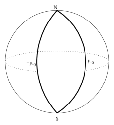
Figure 6: The conformal mapping of the constant time slice is depicted here. Only the surface of the globe described by the $\mu$ and $\lambda$ coordinates is relevant here. Each point on the surface corresponds to $S^{2}$. The boundary indicated by bold lines corresponds to $S^{3}$.

In the pure AdS case, the geometry covers only a half of the surface of the globe; the spatial section of the metric (7) is conformal to $R\times H^{3}$. As shown in the last section, the range of $\mu$ becomes larger as $c_{0}$ grows. There is a value of $c_{0}$ when the range of $\mu$ becomes $\mu\in[-n\pi,n\pi]$ with $n$ being integer, thus the geometry (multiply) covering up the entirety of the globe. But we do still have the boundary, as we do not identify two halves of the boundary –if two halves of the boundary were identified, the spatial section of the geometry would have become (a multi-cover of) $S^{4}$ without boundary. Hence the boundary always consists of two halves of $S^{3}$, independent of the value of $c_{0}$ or equivalently of $\mu_{0}$. As $c_{0}$ approaches its critical value $9/(4\sqrt{2})$, the range of $\mu$ extends to the entire real line.

When we adopt the Poincaré patch for the $AdS_{4}$ slice as in (8), the metric is written as

$$ds^{2}={f(\mu)\over y^{2}}\big{(}-dt^{2}+d\vec{x}^{2}+dy^{2}+y^{2}d\mu^{2}\big{)}\ .$$ (21)

The conformal mapping of the spatial section is depicted in Figure 7. Each point on the plane represents ${R}^{2}$. As in the pure AdS case, $y=\infty$ corresponds to the horizon. Again the boundary is at $\mu=\pm\mu_{0}$. Each of these is a half of ${R}^{3}$, being joined together through the wedge $W$ that is ${R}^{2}$. The range of $\mu$ is the same as before; it becomes larger as $c_{0}$ grows.

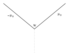
Figure 7: The conformal diagram of the spatial section of our solutions is depicted here for the Poincare type coordinate. Each point on the plane corresponds to ${R}^{2}$. The coordinate $\mu$ is the polar angle and $y$ is the radial coordinate with $W$ as the origin. The total boundary consists of two parts, each of which has the geometry of a half of ${R}^{3}$. These two parts are joined through $W$, which may be viewed as a kind of domain wall on the boundary.

Again the dilaton varies from one constant, $\phi_{0}^{-}=\phi(-\mu_{0})$, at one half of the boundary $\mu=-\mu_{0}$, to another, $\phi_{0}^{+}=\phi(\mu_{0})$, at the other half $\mu=\mu_{0}$, running through the bulk as $\mu$ increases. Hence from the viewpoint of the boundary, the dilaton is constant in each half, taking the value of $\phi_{0}^{+}$ and $\phi_{0}^{-}$ respectively. The discontinuity of the dilaton occurs through the joint $W$. One might worry about possible singularities around the wedge $W$. However, this is just an artifact of the conformal diagram. That is,  from the viewpoint of the original geometry, nothing singular happens around the wedge. The same conclusion follows from the stability analysis as we will see below.

4.1 A comparison to Karch-Randall

In [11] Karch and Randall considered the issue of local localization of gravity on a brane in AdS. In particular they studied $AdS_{4}$ branes in $AdS_{5}$. The geometric picture of their solutions –two ‘halves’ of $AdS_{5}$ glued together along a $AdS_{4}$ brane is quite similar to ours. Note however the differences: We do not have a singular brane source in the bulk. The discontinuity only appears on the boundary.

The coordinate change going from the $AdS_{4}$ slicing

$$ds^{2}_{AdS_{5}}={1\over\cos^{2}\mu}\Big{(}d\mu^{2}+{1\over\cos^{2}\theta}\big{(}-dt^{2}+d\theta^{2}+\sin^{2}\theta d\Omega_{2}^{2}\big{)}\Big{)}$$ (22)

to the standard global $AdS_{5}$ coordinates

$$ds^{2}_{AdS_{5}}=-\cosh^{2}\tilde{r}dt^{2}+d\tilde{r}^{2}+\sinh^{2}\tilde{r}(d\rho^{2}+\sin^{2}\rho d\Omega_{2}^{2})\ ,$$ (23)

is given by

$$\tan{\rho}={\tan\theta\over\sin\mu}\ ,\quad\quad\cosh\tilde{r}={1\over\cos\mu\cos\theta}\ ,$$ (24)

where the range of the coordinates is as follows; For (22) one finds $\mu\in[-\pi/2,\pi/2]$ and $\theta\in[0,\pi/2]$, for (23) one has $\tilde{r}\in[0,\infty]$ and $\rho\in[0,\pi]$. This coordinate system was used to describe the $AdS_{4}$ brane in [11].

In [18] five dimensional gravity coupled to a scalar $\phi$ with potential $V(\phi)$ and a localized co-dimension one brane source, was studied. In section 3.2 the case of an AdS worldvolume of the brane source was studied corresponding to a $AdS_{4}$ slicing of $AdS_{5}$. The dilaton would be a special case where the potential is simply the cosmological constant $V(\phi)=\Lambda$, without any dependence on the dilaton. Note that in our solution there is no singular brane source where the value of fields jump, the solution is more like a (very thick) domain wall.

5 The holographic dual

The solution given by (10), (12), and (15) is very simple, since only the dilaton and the metric develop a nontrivial profile. In this section we will discuss the holographic interpretation of this solution in terms of the theory living on the boundary. The solution breaks the $SO(4,2)$ $AdS_{5}$ symmetry to $SO(3,2)$. Note that this situation is very similar to the $AdS_{4}$ brane in $AdS_{5}$ which displays local localization of gravity [11] and its relation to defect CFT [14][15]. There the reduced AdS symmetry is interpreted as the part of the conformal symmetry group which leaves the defect invariant.

Near the boundary $\mu\to\pm\mu_{0}$, one can easily show that $f(\mu)$ and the dilaton $\phi(\mu)$ behave as follows;

$$f={1\over(\mu\mp\mu_{0})^{2}}+o(1)\ ,\quad\quad\phi=\phi_{0}^{\pm}\mp{c_{0}\over 4}(\mu\mp\mu_{0})^{4}+o((\mu\mp\mu_{0})^{6})\ .$$ (25)

In the standard AdS/CFT dictionary the asymptotic value of the dilaton is identified with the coupling constant of the four dimensional $N=4$ SYM theory living on the boundary. The subleading term is identified with the expectation value for the operator $O_{4}=\mbox{Tr}(F^{2})$. Hence the interpretation of our solution is that the boundary consists of two half spaces, given by $\mu=\pm\mu_{0}$, where the coupling constant is given by

$$\mu=+\mu_{0}:\quad{g_{YM}^{2}\over 4\pi}=e^{\phi_{0}^{+}},\quad\quad\mu=-\mu_{0}:\quad{g_{YM}^{2}\over 4\pi}=e^{\phi_{0}^{-}}\ .$$ (26)

Note however that in our solution we do not need either a potential for the scalar field or a singular brane source in the bulk as in [18].

5.1 Wilson Loops

In [19] it was proposed that the calculation of the expectation value $\langle W(C)\rangle$ of Wilson loop operators in the large $N$ SYM theory,

$$W(C)={1\over N}{\rm tr}Pe^{i\oint_{C}A}\ ,$$ (27)

have a dual holographic interpretation as the minimal area of a fundamental string worldsheet in the AdS bulk, which ends on the boundary. The action for the fundamental string is given by

$$S=-{1\over 2\pi\alpha^{\prime}}\int d\tau d\sigma\sqrt{-det(g_{\mu\nu}\partial_{a}X^{\mu}\partial_{b}X^{\nu})}\ .$$ (28)

Where $g_{\mu\nu}$ is the string frame metric. We assume that the Wilson loop is static and choose the temporal gauge $\tau=X^{0}$, furthermore we assume that the Wilson loop will not depend on the coordinates $x_{i}$. Plugging in the form of the metric (21) one gets for the Lagrangian.

$$L=-\int d\sigma e^{\phi\over 2}{f(\mu)\over y^{2}}\sqrt{\partial_{\sigma}y\partial_{\sigma}y+y^{2}\partial_{\sigma}\mu\partial_{\sigma}\mu}\ .$$ (29)

One can use the remaining reparameterization invariance to choose the static gauge $\mu=\sigma$. The equation of motion following from (29) will be

$$y^{\prime\prime}+y+y^{\prime}\left({f^{\prime}\over f}+{1\over 2}\phi^{\prime}\right)\left(1+{(y^{\prime})^{2}\over y^{2}}\right)=0\ .$$ (30)

Hence the Wilson loop is determined by a set of coupled ordinary differential equations given by (30) together with (12) and (14). The value of the expectation value of the Wilson loop operator is given by $e^{-S}$ for the solution. Using the expansion near the boundary (25), it is easy to see that the action diverges as

$$S\sim e^{\phi_{0}\over 2}|y_{0}|{1\over(\mu\mp\mu_{0})^{2}}+o(1)\ .$$ (31)

This divergence is exactly that of the Wilson loop in AdS [19] and can be regulated by subtracting the (infinite) action of a straight Wilson loop going from the boundary to the horizon.

Figure 8: Wilson line with $c_{0}=1.3$, and $y_{max}=5$.

Unfortunately the equation (30) is too complicated to solve analytically, however numerical solutions are easily obtained. The main feature is that the Wilson loop will be tilted by the nontrivial dilaton profile and metric warping, as can be seen from Figure 8.

6 The stability against small perturbations

Our solution breaks all the supersymmetries of the IIB supergravity. This fact may be checked explicitly by considering the supersymmetry variation of the dilatino and gravitino. Since there is no supersymmetry left unbroken, the background could potentially be unstable. In order to check the stability of our solution against small fluctuations, we shall consider the behavior of the scalar field in the background of our solution. The analysis may be generalized to the metric or R-R field perturbations, but, for simplicity, we shall focus on the case of the scalar field. The stability of a solution requires that there is no configuration with the same or smaller energy into which it can decay. Here we are particularly interested in the perturbative stability of the background and will ask about the following two points:

1) The energy is positive definite for any modes of finite energy satisfying zero momentum flux condition at the boundary. The latter condition i.e. $\int dS_{a}\,T^{a}\!\,_{0}|_{\rm boundary}=0$ is required for the conservation of the energy.

2) One requires the completeness of the modes to allow arbitrary initial configurations of small fluctuation.

In pure AdS space, it is well-known that not too tachyonic scalars are perturbatively stable unlike the case of the flat space. In $AdS_{5}$ the scalar field is stable if the Breitenlohner-Freedman bound is satisfied, $m^{2}\geq-4$. This is the question about the stability of the scalar field itself and the issue here is different from the stability of the background. However as the methods are closely related, we would like to consider the generic massive scalars as well. The $m^{2}=0$ case will then correspond to the stability of the background.

We consider small fluctuations of the scalar field in the background of our solution. Specifically, we work in the Poincare type coordinate,

$$ds^{2}={f(\mu)\over y^{2}}\big{(}-dt^{2}+d\vec{x}^{2}+dy^{2}+y^{2}d\mu^{2}\big{)}\ ,$$ (32)

and consider the equation of motion

$$\left({1\over\sqrt{g}}\partial_{\alpha}\sqrt{g}g^{\alpha\beta}\partial_{\beta}-m^{2}\right)\varphi=0\ ,$$ (33)

for the massive scalar field. Since any inhomogeneous fluctuations in $\vec{x}$ costs more energy, we consider only $\vec{x}$-independent modes. For $\varphi={\rm Re}(e^{-i\omega t}H(\mu,y))$, one finds that the spatial part $H$ satisfies

$$y^{2}\partial_{y}y^{-2}\partial_{y}H+{1\over y^{2}}\left(f^{-{3\over 2}}(\mu)\partial_{\mu}f^{{3\over 2}}(\mu)\,\partial_{\mu}-m^{2}f\right)H=-\omega^{2}H\ .$$ (34)

We solve this by the separation of variables,

$$H=F(\mu)G(y)\ ,$$ (35)

with F($\mu$) satisfying

$$\left(-f^{-{3\over 2}}(\mu)\partial_{\mu}\,f^{{3\over 2}}(\mu)\,\partial_{\mu}+m^{2}f\right)F(\mu)=kF(\mu)\ .$$ (36)

The function $G(y)$ satisfies

$$G^{\prime\prime}-{2\over y}G^{\prime}+(\omega^{2}-k/y^{2})G=0\ ,$$ (37)

which may be solved by

$$G=y^{3/2}Z_{\nu}(\omega y)\ ,$$ (38)

where $\nu^{2}=9/4+k$ and $Z_{\nu}(x)$ is the Bessel function. For real $\omega$, $Z_{\nu}$ may be either $J_{\nu}$ or $N_{\mu}$. When $\omega$ is pure imaginary, we consider only $Z_{\nu}=K_{\nu}(|\omega|y)$ because the other independent solution $I_{\nu}(|\omega|y)$ blows up exponentially at large $y$.

The energy of the system is defined by

$$E={1\over 2}\int dx^{a}\sqrt{g}\left(|g^{00}|\dot{\varphi}^{2}+g^{ab}\partial_{a}\varphi\partial_{b}\varphi+m^{2}\varphi^{2}\right)\ .$$ (39)

Depending on the couplings of the scalar fields to the gravity, there may be a contribution of the improved term [21] to the energy, but here we set this to zero. The inclusion of this contribution will not change the conclusion of our analysis.

For the mode given above, one may formally manipulate the energy functional using integration by parts with respect to $\mu$ and Eq.(36). In the integration by parts, there may be a boundary contribution, but let us assume that the boundary contribution vanishes. The energy functional then becomes

$$E={1\over 2}\int dx^{a}\sqrt{g}g^{yy}\left(\dot{\varphi}^{2}+(\partial_{y}\varphi)^{2}+{k\over y^{2}}\varphi^{2}\right)\ .$$ (40)

When $k+9/4>0$, the second and third term give divergent contributions at small $y$ and the infinities do not cancel if $\varphi\sim y^{3/2}N_{\nu}$ or $y^{3/2}K_{\nu}$. Hence only $\varphi\sim y^{3/2}J_{\nu}(\omega y)$ is allowed by the finiteness when $k+9/4>0$. To show the positivity, we rewrite the energy integral by $S$ defined by $\varphi=y^{3/2+\nu}S$. With a little manipulation, the expression for the energy becomes

$$E={1\over 2}\int dx^{a}\sqrt{g}g^{yy}y^{3+2\nu}\left(\dot{S}^{2}+(\partial_{y}S)^{2}\right)\ ,$$ (41)

for $\varphi\sim y^{3/2}J_{\nu}(\omega y)$. Therefore we conclude that it is sufficient that $k>-9/4$ for the energy of this mode to be positive definite.

Now let us consider the $\mu$-direction where we are interested in the integral

$$I=\int^{\mu_{0}}_{-\mu_{0}}d\mu\,f^{{3\over 2}}\left((\partial_{\mu}F)^{2}+{m^{2}f}F^{2}\right)\ ,$$ (42)

that is the last term of the energy integral (40). Setting $W=Ff^{3/4}$, Eq.(36) becomes

$$[-\partial^{2}_{\mu}+V(f)]W(\mu)=kW(\mu)\ ,$$ (43)

with

$$V={3\over 4f}\left(f^{\prime\prime}-{1\over 4f}f^{\prime}f^{\prime}\right)+m^{2}f={3\over 4}\left(5f-3-{c_{0}^{2}\over 8f^{3}}\right)+m^{2}f\ ,$$ (44)

where, for the second equality, we used (14). We now analyze the equation (36) around $\mu\mp\mu_{0}\sim 0$, and there we have

$$F=(\mu\mp\mu_{0})^{\gamma}(1+{h.\,o.\,t.})\,.$$

Since $f\sim(\mu\mp\mu_{0})^{-2}(1+{h.\,o.\,t.})$, one finds $\gamma(\gamma-4)=m^{2}$ and its solutions are

$$\gamma_{\pm}={2}\pm\sqrt{4+m^{2}}\,.$$

From (42), we see that only $\gamma_{+}$ makes the integral finite when $m^{2}+4\geq 0$.

Let us first consider the $c_{0}=0$ case corresponding to the pure AdS. When $m^{2}+4\geq 0$, with $K=(f^{1\over 2})^{2+\sqrt{4+m^{2}}}F$, the integral $I$ can be rewritten as

$$I=\int^{\pi\over 2}_{-{\pi\over 2}}d\mu\,f^{-\tilde{\gamma}}\left[(K^{\prime})^{2}+(\tilde{\gamma}^{2}-9/4)K^{2}\right]>{-{9\over 4}}\int^{\pi\over 2}_{-{\pi\over 2}}d\mu\,f^{-\tilde{\gamma}}K^{2}\ ,$$ (45)

where $\tilde{\gamma}=1/2+\sqrt{m^{2}+4}$. This can be shown by the integration by parts, in which the boundary contributions vanish. On the other hand, using the equation (36) and integration by parts, one may also be able to show that

$$I=k\int^{\pi\over 2}_{-{\pi\over 2}}d\mu\,f^{-\tilde{\gamma}}K^{2}\ .$$ (46)

Thus we conclude that, for $c_{0}=0$, the condition $k>-9/4$ is not only sufficient but also necessary for the energy of this mode to be finite and positive definite. This way we have shown that the condition $m^{2}+4\geq 0$ is sufficient for the energy to be finite and positive definite. On the other hand, if $m^{2}+4<0$, there may be a mode that has finite energy, but there is no mode satisfying zero momentum flux condition at the boundary $\mu=\pm\mu_{0}$. Then there is no way to satisfy the completeness condition of the modes. In fact, the stability is not about the modes but of an arbitrary initial configuration of small fluctuations. The fact that there is no way to respect the zero flux condition at the boundary in the subsequent time evolution clearly illustrates the instability.

As $c_{0}$ grows, the potential $V(f)$ becomes smaller and the interval $2\mu_{0}$ gets larger. The latter makes the kinetic energy contribution generically smaller. Hence one expects that the mass bound $m^{2}$ will grow as $c_{0}$ gets larger. Unfortunately, the evaluation of the precise bound as a function of $c_{0}$ is not trivial. Hence we will consider the case $c_{0}\rightarrow 9/(4\sqrt{2})$. In this case, we note that the integral $I$ may be written as

$$I=\int^{\mu_{0}}_{-\mu_{0}}d\mu\left((W^{\prime})^{2}+VW^{2}\right)=k\int^{\mu_{0}}_{-\mu_{0}}d\mu\,W^{2}\ ,$$ (47)

for the finite energy modes. Since $\mu_{0}\rightarrow\infty$ the kinetic contribution in (47) can be made arbitrarily small, while making full use of the region where the potential becomes minimal. Namely if one allows an infinitesimal deviation from the minimum, the corresponding range in $\mu$ becomes very large. Hence the evaluation of mass bound follows from the condition that the minimum of the potential should be equal to or larger than $-9/4$. When $m^{2}<-15/4$, the potential is unbounded from below, so we restrict our attention to the case when $m^{2}\geq-15/4$. Then the minimum of the potential is

$$V_{min}={3(3+m^{2})\over 4}-9/4$$

where we have used the fact that the minimum $f_{min}$ of $f$ is given by $3/4$ for $c_{0}=9/(4\sqrt{2})$. This leads to the stability condition $m^{2}\geq-3$ for $c_{0}=9/(4\sqrt{2})$.

From the above analysis, the stability of the background (i.e. the case of $m^{2}=0$) is quite clear. As a by-product, it is convincing that nothing singular happens around $y=0$ contrary to the first impression of the geometrical shape.

In the discussion of stability above, we omitted many details. We do not consider the metric or R-R field perturbations. For the scalar field, we do not include the case where there is the improved term for the energy. As we said earlier, this inclusion will not change our result of stability analysis. We do not present detailed discussion of the zero flux condition, the role of completeness of mode and so on. We leave these issues to the further studies.

7 Discussion

In this note we have presented a very simple deformation of the $AdS_{5}\times S^{5}$ background for type IIB string theory. The main property of the solution is that the AdS space gets ‘elongated’ and the dilaton develops a nontrivial profile. In terms of the representation of $AdS_{d}$ as a hyperboloid in $R^{2,d-1}$ given by (1), the ansatz for the solution simply takes the dilaton to be a function of one of the $X_{i},I=1,\cdots,d-1$. This construction can obviously be generalized to AdS spaces of different dimensionality as long as massless scalar fields are present.

This immediately suggests a generalization of our solution which makes the dilaton a function of one of the timelike coordinates $X_{0}$. The ansatz for the metric, dilaton and five-form is given by

$$ds^{2} = {f(X_{0})\over|1-X_{0}^{2}|}ds_{AdS_{5}}^{2}+ds_{S^{5}}^{2}\ ,$$ (48)

$$\phi = \phi(X_{0})\ ,$$ (49)

$$F_{5} = 4\left({f(X_{0})^{5/2}\over|1-X_{0}^{2}|^{5/2}}\omega_{AdS_{5}}+\omega_{S^{5}}\right)\ .$$ (50)

The equation of motion determines $f(X_{0})$

$$\phi^{\prime}(X_{0}) = c_{0}|1-X_{0}^{2}|^{1/2}f^{-3/2}\ ,$$ (51)

$$(1-X_{0}^{2})^{2}f^{\prime 2} = 4f^{2}-4{1-X_{0}^{2}\over|1-X_{0}^{2}|}f^{3}+{c_{0}^{2}\over 6}f^{-1}\ .$$ (52)

For $c_{0}\neq 0$ there are two branches of the solution with $X_{0}^{2}>1$ and $X_{0}^{2}<1$. Note that in contrast to to the spacelike case discussed in section 3, $f$ reaches zero in finite time. Since the scalar curvature is given by

$$R=-20-{c_{0}^{2}\over 2f^{4}}\ .$$ (53)

This implies that this solution has naked singularities. For the branch $X_{0}^{2}>1$ this is a timelike singularity whereas for $X_{0}^{2}<1$ it is a spacelike singularity. Note also that in the second case $f$ does not reach infinity and hence there is no boundary.

It is an open and very interesting question whether this singularity can be resolved or given a proper interpretation (as an unstable decaying brane and a cosmology respectively) in the full string theory.

Finally note that, in finding our gravity solution, we make use of the unbroken $SO(3,2)$ invariance to simplify the equations of motion. However, the ansatz we used is not the most general one consistent with the $SO(3,2)$ symmetry. Any generalization of our ansatz with the symmetry would be quite interesting. In particular, this may be helpful in finding the supergravity solutions of the $AdS_{4}\times S^{2}$ branes in $AdS_{5}\times S^{5}$ with inclusion of full back reaction.

References

- [1] J. M. Maldacena, “The large N limit of superconformal field theories and supergravity,” Adv. Theor. Math. Phys. 2, 231 (1998) [Int. J. Theor. Phys. 38, 1113 (1999)] [arXiv:hep-th/9711200].
- [2] S. S. Gubser, I. R. Klebanov and A. M. Polyakov, “Gauge theory correlators from non-critical string theory,” Phys. Lett. B 428, 105 (1998) [arXiv:hep-th/9802109].
- [3] E. Witten, “Anti-de Sitter space and holography,” Adv. Theor. Math. Phys. 2, 253 (1998) [arXiv:hep-th/9802150].
- [4] G. ’t Hooft, “Dimensional Reduction In Quantum Gravity,” arXiv:gr-qc/9310026.
- [5] L. Susskind, “The World as a hologram,” J. Math. Phys. 36, 6377 (1995) [arXiv:hep-th/9409089].
- [6] O. Aharony, S. S. Gubser, J. M. Maldacena, H. Ooguri and Y. Oz, “Large N field theories, string theory and gravity,” Phys. Rept. 323, 183 (2000) [arXiv:hep-th/9905111].
- [7] A. Kehagias and K. Sfetsos, “On asymptotic freedom and confinement from type-IIB supergravity,” Phys. Lett. B 456 (1999) 22 [arXiv:hep-th/9903109].
- [8] A. Kehagias and K. Sfetsos, “On running couplings in gauge theories from type-IIB supergravity,” Phys. Lett. B 454 (1999) 270 [arXiv:hep-th/9902125].
- [9] S. S. Gubser, “Dilaton-driven confinement,” arXiv:hep-th/9902155.
- [10] L. Girardello, M. Petrini, M. Porrati and A. Zaffaroni, “Confinement and condensates without fine tuning in supergravity duals of gauge theories,” JHEP 9905 (1999) 026 [arXiv:hep-th/9903026].
- [11] A. Karch and L. Randall, “Locally localized gravity,” JHEP 0105, 008 (2001) [arXiv:hep-th/0011156].
- [12] M. Porrati, “Mass and gauge invariance. IV: Holography for the Karch-Randall model,” Phys. Rev. D 65 (2002) 044015 [arXiv:hep-th/0109017].
- [13] M. Porrati, “Higgs phenomenon for 4-D gravity in anti de Sitter space,” JHEP 0204 (2002) 058 [arXiv:hep-th/0112166].
- [14] A. Karch and L. Randall, “Open and closed string interpretation of SUSY CFT’s on branes with boundaries,” JHEP 0106, 063 (2001) [arXiv:hep-th/0105132].
- [15] O. DeWolfe, D. Z. Freedman and H. Ooguri, “Holography and defect conformal field theories,” Phys. Rev. D 66, 025009 (2002) [arXiv:hep-th/0111135].
- [16] C. Bachas, J. de Boer, R. Dijkgraaf and H. Ooguri, “Permeable conformal walls and holography,” JHEP 0206, 027 (2002) [arXiv:hep-th/0111210].
- [17] O. Aharony, O. DeWolfe, D. Z. Freedman and A. Karch, “Defect conformal field theory and locally localized gravity,” arXiv:hep-th/0303249.
- [18] O. DeWolfe, D. Z. Freedman, S. S. Gubser and A. Karch, “Modeling the fifth dimension with scalars and gravity,” Phys. Rev. D 62, 046008 (2000) [arXiv:hep-th/9909134].
- [19] J. M. Maldacena, “Wilson loops in large N field theories,” Phys. Rev. Lett. 80, 4859 (1998) [arXiv:hep-th/9803002]; S. J. Rey and J. Yee, “Macroscopic strings as heavy quarks in large N gauge theory and anti-de Sitter supergravity,” Eur. Phys. J. C 22, 379 (2001) [arXiv:hep-th/9803001].
- [20] A. Karch and L. Randall, “Localized gravity in string theory,” Phys. Rev. Lett. 87, 061601 (2001) [arXiv:hep-th/0105108].
- [21] P. Breitenlohner and D. Z. Freedman, “Positive Energy In Anti-De Sitter Backgrounds And Gauged Extended Supergravity,” Phys. Lett. B 115, 197 (1982); G. W. Gibbons, C. M. Hull and N. P. Warner, Nucl. Phys. B 218, 173 (1983); L. Mezincescu and P. K. Townsend, Annals Phys. 160, 406 (1985).