RUNHETC-2003-10

Exact solutions for supersymmetric stationary black hole composites


Brandon Bates 1 and Frederik Denef 2


1 Department of Physics, Columbia University

New York, NY 10027, USA

bdbates@phys.columbia.edu


2 Department of Physics and Astronomy, Rutgers University

Piscataway, NJ 08855-8019, USA

denef@physics.rutgers.edu

Abstract


Four dimensional ${\cal N}=2$ supergravity has regular, stationary, asymptotically flat BPS solutions with intrinsic angular momentum, describing bound states of separate extremal black holes with mutually nonlocal charges. Though the existence and some properties of these solutions were established some time ago, fully explicit analytic solutions were lacking thus far. In this note, we fill this gap. We show in general that explicit solutions can be constructed whenever an explicit formula is known in the theory at hand for the Bekenstein-Hawking entropy of a single black hole as a function of its charges, and illustrate this with some simple examples. We also give an example of moduli-dependent black hole entropy.

1 Introduction

The analysis of BPS states in various compactifications of string theory has been of fundamental importance in exploring non-perturbative phenomena, dualities and quantum geometry. In particular in type II theory compactified on a Calabi-Yau threefold, where BPS states have a description as D-branes wrapped on various supersymmetric cycles (and generalizations thereof), this study has revealed some remarkable physical and mathematical structures. The low energy effective theory of such a Calabi-Yau compactification is a four-dimensional ${\cal N}=2$ supergravity theory, coupled to a number of massless abelian vector- and hypermultiplets, and in this theory BPS states have a description complementary to the D-brane picture as solutions to the field equations preserving ${\cal N}=1$ supersymmetry. The simplest solutions of this kind are spherically symmetric black holes, first studied in [1]. As noted in [2], not all charges support such solutions. This is natural, since also in the full string theory, the BPS spectrum is only a subset of the full charge lattice. However, it turns out that the true BPS spectrum and the spectrum of spherically symmetric black holes do not match [3, 4], the latter being too small. To reconcile the two, one has to drop the restricion to spherically symmetric solutions with a single charge center, and consider multicentered composites as well [4]. Indeed, ${\cal N}=2$ supergravity has regular BPS “bound state” solutions describing configurations of distinct (typically mutually nonlocal) charges at rest at certain equilibrium separations from each other. These solutions are in general stationary but non-static, as they can carry an intrinsic angular momentum, much like the monopole-electron system in ordinary Maxwell electrodynamics. Furthermore their existence is subject to certain moduli-dependent stability conditions, matching similar conditions appearing in the D-brane description of BPS states [5, 6, 7]. With these ingredients, supergravity predictions for the BPS spectrum of the full string theory were given in [8].

The equations of motion for general stationary BPS configurations were derived in [9, 4, 10]. In [4], non-static black hole composites were considered as solutions, and some of their properties were analyzed directly from the equations, assuming existence. A proof of existence was later given in [12], however without giving explicit analytic expressions for the metric, scalars and vectors. In what follows, we will show how such closed form expressions can be found. Perhaps somewhat surprisingly, it turns out that the full solution can be built from a single function, namely the Bekenstein-Hawking entropy (i.e. the horizon area) of a single BPS black hole as a function of its charges. If the latter is known analytically, the same is true for the complete space-time geometry and all fields involved, for arbitrary values of the moduli at spatial infinity.

Some examples of non-static multicentered solutions were studied earlier in [11], for supergravity with $R^{2}$-corrections, focusing mainly on how to take the curvature corrrections into account in an iterative approximation scheme. The zeroth order part of those results can be obtained as a special case of the general construction outlined in this note. An explicit expression for the off-diagonal part of the metric was not given in [11]. We show how this part can be obtained in closed form without too much additional effort, and note that requiring its regularity leads to constraints on the positions of the centers and to certain stability conditions, confirming general expectations [4].

2 Notation and setup

2.1 General formalism

We will assume that the supergravity theory under consideration arises from compactification of type IIB string theory on a Calabi-Yau threefold, thus giving a concrete geometric interpretations to the various quantities involved. The generalization to arbitrary supergravity theories determined by abstract special geometry data will be obvious.

Compactification of IIB on a Calabi-Yau manifold $X$ gives as four-dimensional low energy theory ${\cal N}=2$ supergravity coupled to $n_{v}=h^{1,2}(X)$ massless abelian vectormultiplets and $n_{h}=h^{1,1}(X)+1$ massless hypermultiplets, where the $h^{i,j}(X)$ are the Hodge numbers of $X$. The hypermultiplet fields will play no role in the following and are set to arbitrary constant values.

The complex scalars in the vector multiplets are the complex structure moduli of $X$. The geometry of the corresponding scalar moduli space ${\cal M}$, parametrized with $n_{v}$ coordinates $z^{a}$, is special Kähler [13]. In what follows we recall some general facts and useful formulas in special geometry (in the IIB geometric setting).

The basic objects in special geometry are $(i)$ a vector space $V$, here identified with the $2n_{v}+2$ dimensional vector space of harmonic 3-forms $H^{3}(X,\mathbb{C})$, for which we pick an arbitrary basis $\{\Theta_{A}\}$; $(ii)$ an antisymmetric bilinear form $\langle\cdot,\cdot\rangle$, here identified with the intersection product on $H^{3}(X,\mathbb{C})$,

$$\langle Q_{1},Q_{2}\rangle=\int_{X}Q_{1}\wedge Q_{2}=Q_{1}^{A}\,I_{AB}\,Q_{2}^{B},\quad\mbox{where }I_{AB}=\langle\Theta_{A},\Theta_{B}\rangle;$$ (2.1)

and $(iii)$ a $V$-valued holomorphic function111single-valued only on the covering space $\widetilde{{\cal M}}$ of ${\cal M}$, here identified with the holomorphic 3-form on $X$,

$$\Omega_{0}(z)=\Omega_{0}^{A}(z)\,\Theta_{A}=I^{AB}X_{B}(z)\,\Theta_{A},\quad\mbox{where }X_{A}=\langle\Theta_{A},\Omega_{0}\rangle=\int_{\widetilde{\Theta}_{A}}\Omega_{0},$$ (2.2)

with $I^{AB}\equiv(I^{-1})^{AB}$ and $\widetilde{\Theta}_{A}$ the 3-cycle Poincaré dual to $\Theta_{A}$. The vector $X_{A}$ is called the holomorphic period vector.

The special Kähler metric $g_{a\bar{b}}=\partial_{a}\bar{\partial}_{\bar{b}}{\cal K}$ on ${\cal M}$ is derived from the Kähler potential

$${\cal K}(z,\bar{z})=-\ln i\langle\Omega_{0},\bar{\Omega}_{0}\rangle=-\ln\left(i\,\bar{X}_{A}I^{AB}X_{B}\right).$$ (2.3)

It is useful to introduce also the normalized 3-form and period vector

$$\Omega=e^{{\cal K}/2}\Omega_{0},\qquad Z_{A}=e^{{\cal K}/2}X_{A}$$ (2.4)

Note that $Z_{A}$ has non-holomorphic dependence on the moduli through ${\cal K}$. The Kähler covariant derivative $D_{a}$ is defined on these normalized objects as $D_{a}\equiv\partial_{a}+\partial_{a}{\cal K}/2$. Then $D_{a}\Omega\in H^{2,1}(X)$, and since $\Omega\in H^{3,0}(X)$, one has $\langle\Omega,D_{a}\Omega\rangle=0$, $\langle\bar{\Omega},D_{a}\Omega\rangle=0$. Furthermore

$$\langle\Omega,\bar{\Omega}\rangle=-i,\qquad\langle D_{a}\Omega,\bar{D}_{\bar{b}}\bar{\Omega}\rangle=i\,g_{a\bar{b}}.$$ (2.5)

The low energy dynamics of the vector fields is also determined by special geometry. The type IIB self-dual five-form field strength ${\cal F}=d{\cal A}$ descends to the four dimensional electromagnetic field strengths $F^{I}=dA^{I}$ and their magnetic duals $G_{I}$ by the decomposition ${\cal F}=F^{I}\otimes\beta_{I}-G_{I}\otimes\alpha^{I}$, where $\{\alpha^{I},\beta_{I}\}_{I=1,\ldots,n_{v}+1}$ is a fixed standard $\langle\cdot,\cdot\rangle$-symplectic basis222i.e. $\langle\alpha^{I},\beta_{J}\rangle=\delta^{I}_{J}$ and $\langle\alpha_{I},\alpha_{J}\rangle=\langle\beta^{I},\beta^{J}\rangle=0$. of harmonic 3-forms on $X$. The fields $G_{I}$ and $F^{I}$ are not independent: they are related by the self-duality constraint on ${\cal F}$.In the four dimensional context, we refer to the $H^{3}(X,\mathbb{R})$-valued field ${\cal F}$ as the total electromagnetic field strength.

The lattice of electric and magnetic charges is identified with $H^{3}(X,\mathbb{Z})$. The origin of a charge $\Gamma\in H^{3}(X,\mathbb{Z})$ in type IIB string theory (at $g_{s}\to 0$) is a D3-brane wrapped around the cycle Poincaré dual to $\Gamma$.

2.2 Example: diagonal $T^{6}$

Let $X_{\tau}$ be the diagonal $T^{6}$ [2] with modulus $\tau$, that is, $X_{\tau}=E_{\tau}\times E_{\tau}\times E_{\tau}$, where $E_{\tau}$ is the 2-torus with standard complex structure parameter $\tau=b+ia$ (valued in the upper half plane). This gives a consistent truncation of the full $\mbox{IIB}/T^{6}$ theory, if moreover we only consider charges $\Gamma\in H^{3}(X,\mathbb{Z})$ invariant under the permutation symmetry of the three 2-tori.

Type IIB string theory on $X_{\tau}$ is mirror (or T-dual333By T-dualizing along the horizontal direction in each $T^{2}$) to IIA on $Y=E^{\prime}_{\tau}\times E^{\prime}_{\tau}\times E^{\prime}_{\tau}$, with $E^{\prime}_{\tau}$ the 2-torus with area $a={\rm Im}\,\tau$ and $B$-field flux $b={\rm Re}\,\tau$ (which together determine the complexified Kähler class of $Y$). There are four charges $\Gamma\in H^{3}(X,\mathbb{Z})$ invariant under the permutation symmetry, mirror to D0-, D2-, D4- and D6-branes on the IIA side. Denoting the standard complex coordinate in the $i$-th $T^{2}$ by $z^{i}=u^{i}+\tau v^{i}$, these charges are explicitly:

$\displaystyle D0$ $\displaystyle\leftrightarrow$ $\displaystyle-dv^{1}\wedge dv^{2}\wedge dv^{3}$ (2.6)
$\displaystyle D2$ $\displaystyle\leftrightarrow$ $\displaystyle dv^{1}\wedge dv^{2}\wedge du^{3}+dv^{1}\wedge du^{2}\wedge dv^{3}+du^{1}\wedge dv^{2}\wedge dv^{3}$ (2.7)
$\displaystyle D4$ $\displaystyle\leftrightarrow$ $\displaystyle-du^{1}\wedge du^{2}\wedge dv^{3}-du^{1}\wedge dv^{2}\wedge du^{3}-dv^{1}\wedge du^{2}\wedge du^{3}$ (2.8)
$\displaystyle D6$ $\displaystyle\leftrightarrow$ $\displaystyle du^{1}\wedge du^{2}\wedge du^{3}.$ (2.9)

The holomorphic 3-form on $X$ is $\Omega=dz^{1}\wedge dz^{2}\wedge dz^{3}$. With respect to the (D0,D2,D4,D6)-basis, the period vector is $X=(1,3\tau,-3\tau^{2},-\tau^{3})$. So the D0-brane is mirror to a D3-brane wrapped in the $u^{i}$-directions, and so on. The intersection matrix is

$$I=\left(\begin{array}[]{cccc}0&0&0&1\\ 0&0&-3&0\\ 0&3&0&0\\ -1&0&0&0\end{array}\right),$$ (2.10)

the special Kähler potential on moduli space is ${\cal K}=-\ln(8a^{3})$, and the corresponding metric is $g_{\tau\bar{\tau}}=3/4a^{2}$.

3 BPS equations of motion

In this section we recall the BPS field equations for a general stationary black hole composite. The ${\cal N}=2$ supergravity plus vector multiplet action is, in units with $G_{N}=1$,

$$S_{4d}=\frac{1}{16\pi}\int d^{4}x\sqrt{-h}R\,-\,2g_{a\bar{b}}\,dz^{a}\wedge*d\bar{z}^{\bar{b}}\,\,-F^{I}\wedge G_{I}\,.$$ (3.1)

The action for a probe BPS particle of charge $\Gamma$ is

$$S_{p}=-\int|Z|\,ds+\frac{1}{2}\int\langle\Gamma,{\cal A}\rangle,$$ (3.2)

where $Z=Z_{\Gamma}=\Gamma^{A}Z_{A}$. providing a source for the fields in (3.1). A BPS metric is of the form

$$ds^{2}=e^{2U}\left(dt+\omega_{i}dx^{i}\right)^{2}-e^{-2U}dx^{i}dx^{i}\,,$$ (3.3)

where $U$ and $\omega$, together with the moduli fields $z^{a}$, are time-independent solutions of the following equations [4, 10]:

$\displaystyle 2e^{-U}{\rm Im}\left(e^{-i\alpha}\Omega\right)$ $\displaystyle=$ $\displaystyle-H\,,$ (3.4)
$\displaystyle\boldsymbol{*}d\omega$ $\displaystyle=$ $\displaystyle\langle dH,H\rangle\,,$ (3.5)

with $\alpha$ an unknown real function, $H({\bf x})$ a given $H^{3}(X,\mathbb{R})$-valued harmonic function (on flat coordinate space $\mathbb{R}^{3}$), and $\boldsymbol{*}$ the Hodge star operator on flat $\mathbb{R}^{3}$. For $N$ charges $\Gamma_{s}$ located at coordinates ${\bf x}_{s}$, $p=1,\ldots,N$, in asymptotically flat space, one has:

$$H=\sum_{s=1}^{N}\frac{\Gamma_{s}}{|{\bf x}-{\bf x}_{s}|}\,\,-\,2{\rm Im}\left(e^{-i\alpha}\Omega\right)_{r=\infty}\,.$$ (3.6)

The boundary condition on $\alpha$ at $r=\infty$ is that it equals the phase of the total central charge, $\alpha=\arg Z_{\Gamma}$, with $Z_{\Gamma}=\Gamma^{A}Z_{A}$ and $\Gamma=\sum_{s}\Gamma_{s}$.

The total electromagnetic field ${\cal F}=d{\cal A}$ is furthermore given by

$${\cal A}=2e^{U}{\rm Re}\left(e^{-i\alpha}\Omega\right)(dt+\omega)+{\cal A}_{d},$$ (3.7)

where ${\cal A}_{d}$ is a Dirac magnetic monopole type vector potential obtained from

$$d{\cal A}_{d}=-2\boldsymbol{*}d\left(e^{-U}{\rm Im}\left(e^{-i\alpha}\Omega\right)\right)=\boldsymbol{*}dH$$ (3.8)

Not all positions of the charges are allowed [4], as equation (3.5) leads to an integrability condition, obtained by acting with $d\boldsymbol{*}$ on both sides of the equation: for all $s=1,\dots,N$

$$\sum_{t=1}^{N}\frac{\langle\Gamma_{s},\Gamma_{t}\rangle}{|{\bf x}_{s}-{\bf x}_{t}|}=2\,{\rm Im}\left(e^{-i\alpha}Z_{s}\right)_{r=\infty}.$$ (3.9)

In the case of just two charges $\Gamma_{1}$ and $\Gamma_{2}$, this simplifies to

$$|{\bf x}_{1}-{\bf x}_{2}|=\frac{\langle\Gamma_{1},\Gamma_{2}\rangle}{2\,{\rm Im}(e^{-i\alpha}Z_{1})_{r=\infty}}\,.$$ (3.10)

Obviously, the separation has to be positive, so positivity of the right hand side gives a necessary condition on the moduli at spatial infinity for existence of a solution. It is indeed common in ${\cal N}=2$ theories for BPS states to exist only in certain regions of moduli space. When one goes from a region where the state exist to one where it doesn’t, the BPS state decays into its constituents, which is energetically only possible on a wall of marginal stability, where the phases of the central charges of the constituents align, that is $\arg Z_{1}=\arg Z_{2}$. From (3.10) it follows indeed that the separation diverges when such a wall is approached.

4 Solutions

4.1 Solutions for $U$ and $z$: general case

We now turn to the construction of explicit solutions. We start by showing that if we use certain preferred holomorphic coordinates on $\widetilde{{\cal M}}$, solutions to (3.4) can be expressed in terms of a single function $\Sigma$ on $H^{3}(X,\mathbb{R})$, proportional to the Bekenstein-Hawking entropy function. Consider first more generally for an arbitrary $Q\in H^{3}(X,\mathbb{R})$ the equation

$$2\,{\rm Im}(\bar{C}\Omega)=-Q$$ (4.1)

in $n_{v}+1$ unknown complex variables, $z^{a}$ and $C$. Expressed in components by computing intersection products with a basis $\{\Theta_{A}\}$, this becomes

$$2\,{\rm Im}(\bar{C}Z_{A})=-I_{AB}Q^{B}.$$ (4.2)

These are $2n_{v}+2$ real equations, so we can in general expect a finite number of solutions $C_{*}(Q)$, $z_{*}(Q)$ for a given $Q$. Now note that by taking the intersection product of (4.1) with $\Omega$ and using $\langle\bar{\Omega},\Omega\rangle=i$, we get $C_{*}(Q)=Z_{Q}|_{z_{*}(Q)}=Q^{A}Z_{A}|_{z_{*}(Q)}$, while taking intersection products with $D_{a}\Omega$ and using $\langle\Omega,D_{a}\Omega\rangle=\langle\bar{\Omega},D_{a}\Omega\rangle=0$ results in $Q^{A}\,D_{a}Z_{A}|_{z_{*}(Q)}=0$, which in turn implies $\partial_{a}|Q^{A}Z_{A}|^{2}|_{z_{*}(Q)}=0$. Similarly $\bar{\partial}_{\bar{a}}|Q^{A}Z_{A}|^{2}|_{z_{*}(Q)}=0$. Defining the function444If the solution $C_{*}(Q)$, $z_{*}(Q)$ is not unique, $\Sigma(Q)$ will be multi-valued. This will generically be the case when ${\cal M}$ has conifold-type singularities [8]. Also, for a range values of $Q$, there may be no solution at all.

$$\Sigma(Q)\equiv|Q^{A}Z_{A}|^{2}|_{z_{*}(Q)}=|C_{*}(Q)|^{2},$$ (4.3)

we have

$\displaystyle\frac{\partial\Sigma}{\partial Q^{A}}$ $\displaystyle=$ $\displaystyle\left.\frac{\partial|Q^{A}Z_{A}|^{2}}{\partial Q^{A}}\right|_{z_{*}(Q)}+\partial_{a}|Q^{A}Z_{A}|^{2}|_{z_{*}(Q)}\,\frac{\partial z_{*}^{a}}{\partial Q^{A}}+\bar{\partial}_{\bar{a}}|Q^{A}Z_{A}|^{2}|_{z_{*}(Q)}\,\frac{\partial\bar{z}_{*}^{\bar{a}}}{\partial Q^{A}}$
$\displaystyle=$ $\displaystyle(\bar{Z}_{Q}Z_{A}+Z_{Q}\bar{Z}_{A})|_{z_{*}(Q)}+0+0$
$\displaystyle=$ $\displaystyle 2\,{\rm Re}(\bar{C}_{*}Z_{A}|_{z_{*}(Q)}).$

Therefore we find that a solution to (4.1) for a given $Q$ satisfies

$$2\bar{C}Z_{A}=\partial_{A}\Sigma-i\,I_{AB}Q^{B},$$ (4.4)

and, since $Z_{A}=e^{{\cal K}/2}X_{A}$:

$$t_{A}\equiv\frac{X_{A}}{X_{0}}=\frac{\partial_{A}\Sigma-i\,I_{AB}Q^{B}}{\partial_{0}\Sigma-i\,I_{0B}Q^{B}},$$ (4.5)

where the 00-index refers to some suitably chosen basis element. Locally, $n_{v}$ of the $t_{A}$ can be used as holomorphic coordinates on $\widetilde{{\cal M}}$. They are the usual “special” coordinates of special geometry. Thus, (4.5) together with (4.3) gives the values for $|C|$ and the moduli solving (4.1) in terms of a single function $\Sigma$ (which of course may still be hard to compute). Note that $\Sigma$ is a homogeneous function of degree two, i.e. $\Sigma(\lambda Q)=\lambda^{2}\Sigma(Q)$, since (4.4) implies

$$Q^{A}\partial_{A}\Sigma=2\bar{C}Q^{A}Z_{A}=2|Q^{A}Z_{A}|^{2}=2\Sigma.$$ (4.6)

Now we apply all this to solve the BPS field equation (3.4), which is of the form (4.1) with $Q=H({\bf x})$ and $C=e^{-U({\bf x})}e^{i\alpha({\bf x})}$, so

$$e^{-2U}=\Sigma(H)\quad\mbox{ and }\quad t_{A}\equiv\frac{X_{A}}{X_{0}}=\frac{\partial_{A}\Sigma(H)-i\,I_{AB}H^{B}}{\partial_{0}\Sigma(H)-i\,I_{0B}H^{B}}.$$ (4.7)

If $\Sigma$ is multi-valued, the relevant branch is selected by continuity and the fact that the solution is unambiguous at infinity (since it is given by the boundary conditions). An obvious necessary condition for existence of the solution is furthermore that $H$ stays within the domain of $\Sigma$ everywhere.

To connect $\Sigma$ to the Bekenstein-Hawking entropy, consider the case of a single charge $\Gamma$ at the origin, i.e. $H=\Gamma/r-C$. Then we find for the horizon area of the BPS black hole thus produced, from (4.7) and the degree two homogeneity property of $\Sigma$:

$$A=4\pi\lim_{r\to 0}r^{2}e^{-2U}=4\pi\lim_{r\to 0}r^{2}\Sigma(\Gamma/r-C)=4\pi\Sigma(\Gamma),$$ (4.8)

and therefore for the Bekenstein-Hawking entropy function $S_{BH}$

$$S_{BH}(\Gamma)=\pi\Sigma(\Gamma).$$ (4.9)

So we see that if $S_{BH}$ is explicitly known, the full solution (for $U$ and the moduli in special coordinates) can be constructed explicitly as well. As a side remark, note that homogeneity of $\Sigma$ and (4.7) similarly imply that the moduli at the horizon $r=0$ are fixed to the value obtained by replacing $H\to\Gamma$ in the expression for $t_{A}$, and in particular are independent of the moduli at infinity (apart for possible $\Sigma$-branch selection). This is the well-known attractor mechanism of ${\cal N}=2$ BPS black holes [1].

Computing $S_{BH}$ in ${\cal N}=2$ supergravity theories analytically can be quite involved, and has only been done in limits where the periods become polynomial in the special coordinates (e.g. large complex structure (radius) limits in compactification of IIB (IIA) on a Calabi-Yau) [14, 2]. This usually proceeds through solving an equation of the form (4.1) (with $Q=\Gamma$), and along the way one derives the corresponding expressions for the $t_{A}$ as well. In practice it is often more convenient to directly use those formulas rather than computing the $t_{A}$ from $\Sigma$ using (4.7). The only point of this section is then the prescription that the full solution is obtained from the horizon computations essentially by substituting the harmonic function $H$ for the charge $\Gamma$.

Alternatively, in some cases, one can compute the entropy function microscopically [15, 16, 17]. Then this section gives a recipe to construct the full supergravity solution just from this piece of microscopic information. In fact, using (4.5), one can in principle reconstruct the full special geometry from knowledge of the entropy function alone.

4.2 Solutions for $U$ and $z$: diagonal $T^{6}$ example

In the case of the diagonal $T^{6}$ example of section 2.2, the function $\Sigma$ is given by $\Sigma(Q)=\sqrt{D(Q)}$, with $D(Q)$ the discriminant function [2]:

$$D=3p^{2}q^{2}+4p^{3}u+4q^{3}v+6uqpv-u^{2}v^{2}$$ (4.10)

where we have denoted the components of $Q$ with respect to the $(D0,D2,D4,D6)$-basis as $(u,q,p,v)$, so $Q^{A}X_{A}=u+3q\tau-3p\tau^{2}-v\tau^{3}$. For the corresponding modulus $\tau=b+a\,i$ we get (using (4.5) or directly from [2]):

$$\tau=b+a\,i=\frac{pq-uv+i\sqrt{D}}{2(p^{2}+qv)}.$$ (4.11)

For charges $\Gamma_{s}=(\hat{u}_{s},\hat{q}_{s},\hat{p}_{s},\hat{v}_{s})$ at positions ${\bf x}_{s}$, the harmonic function $H$ of (3.6) is, with $r_{s}\equiv|{\bf x}-{\bf x}_{s}|$:

$\displaystyle H({\bf x})$ $\displaystyle=$ $\displaystyle\biggl{(}u({\bf x}),q({\bf x}),p({\bf x}),v({\bf x})\biggr{)}$ (4.12)
$\displaystyle=$ $\displaystyle\biggl{(}\mbox{$\sum_{s}$}\frac{\hat{u}_{s}}{r_{s}}-c_{0},\mbox{$\sum_{s}$}\frac{\hat{q}_{s}}{r_{s}}-c_{2},\mbox{$\sum_{s}$}\frac{\hat{p}_{s}}{r_{s}}-c_{4},\mbox{$\sum_{s}$}\frac{\hat{v}_{s}}{r_{s}}-c_{6}\biggr{)},$ (4.13)

where

$$(c_{0},c_{2},c_{4},c_{6})=\frac{2}{\sqrt{8a^{3}}}{\rm Im}[e^{-i\alpha}(\tau^{3},-\tau^{2},-\tau,1)]\,\,\biggr{|}_{r=\infty}$$ (4.14)

and $\alpha=\arg(\hat{u}+3\hat{q}\tau-3\hat{p}\tau^{2}-\hat{v}\tau^{3})$ with $(\hat{u},\hat{q},\hat{p},\hat{v})=\sum_{s}(\hat{u}_{s},\hat{q}_{s},\hat{p}_{s},\hat{v}_{s})$. The metric factor $e^{-2U}$ of the solution is then obtained as $e^{-2U({\bf x})}=\sqrt{D({\bf x})}$ with the ${\bf x}$-dependent $(u,q,p,v)$ from (4.13) plugged into (4.10), and the modulus field $\tau({\bf x})$ similarly from (4.11).

Note that for the solution to exist, we need $D\geq 0$ everywhere. In particular this requires $D(\Gamma_{s})\geq 0$ for all charges $\Gamma_{s}$. Recall furthermore that the constraint (3.9) has to be satisfied.

A simple spherically symmetric example is provided by considering a charge $(\hat{u},0,\hat{p},0)$, $\hat{u},\hat{p}>0$, with $\tau_{\infty}=ia_{\infty}$. Then we get $e^{-2U}=\sqrt{D}=2\sqrt{p^{3}u}$, $\tau=i\sqrt{u/p}$, with $u=\hat{u}/r+\sqrt{a_{\infty}^{3}/2}$, $p=\hat{p}/r+1/\sqrt{2a_{\infty}}$, reproducing the usual D0-D4 BPS black hole solution with zero $B$-field.

Refer to caption
Figure 1: Left: Profile of $\tau({\bf x})$ in the upper half plane for the 2-centered example described in the text. The shaded region is the domain of allowed values of $\tau_{\infty}$. The red curve is the line of marginal stability. Right: $e^{U}$ as a function of $x$ with the two charges located on the $x$-axis.

As a specific example of a two-centered solution, consider the charges $\Gamma_{1}=(4,0,1,0)$ and $\Gamma_{2}=(0,4,0,1)$. Notice that $D(\Gamma_{1})=D(\Gamma_{2})=16$ while $D(\Gamma_{1}+\Gamma_{2})=-125$, so a two-centered solution can indeed exist whereas a single centered one cannot. From (3.10), we find for the separation of the charges

$$|{\bf x}_{1}-{\bf x}_{2}|=-19\sqrt{2a}|X|\,/\,(12a^{4}+12b^{4}+24a^{2}b^{2}+25a^{2}-39b^{2}+12)\biggr{|}_{r=\infty}$$ (4.15)

with $X=X_{1}+X_{2}=4+12\tau-3\tau^{2}-\tau^{3}$. Therefore a necessary condition for existence of the solution is

$$12a^{4}+12b^{4}+24a^{2}b^{2}+25a^{2}-39b^{2}+12<0.$$ (4.16)

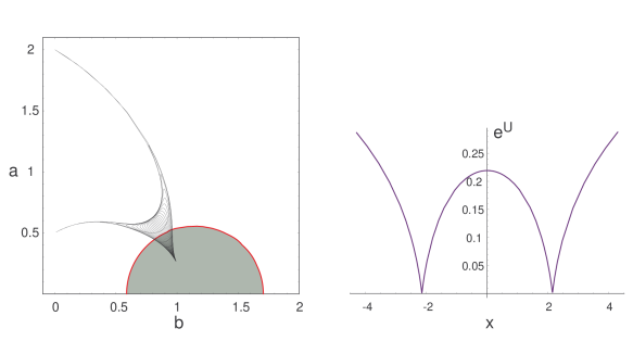
The zero locus of the left hand side consists of two branches, one with $b>0$ (shown in fig. 1) and the other with $b<0$. On the $b<0$ branch, we have $\arg Z_{1}=\arg Z_{2}+\pi$, and on the $b>0$ branch, we have $\arg Z_{1}=\arg Z_{2}$. As discussed at the end of section 3, on general grounds, only the latter branch can be a boundary between a region where the BPS state exists and a region where it does not. Therefore, the only region in which the BPS bound state can exist is the region inside the branch with $b>0$.555When one tries to construct a solution with $\tau$ at $r=\infty$ inside the other branch, one finds that $D$ becomes negative and the solution breaks down.

To be completely explicit, let us pick the point $b=1$, $a=1/4$, which lies inside the stable domain. The separation of the charges is then $|{\bf x}_{1}-{\bf x}_{2}|\approx 4.29899$, and

$$H\approx(\frac{4}{r_{1}}-5.47809,\frac{4}{r_{2}}+5.83671,\frac{1}{r_{1}}+5.83091,\frac{1}{r_{2}}-5.48245).$$ (4.17)

The corresponding image of the map $\tau({\bf x})$ is plotted in fig. 1. It has the profile of a “fattened split flow”, as anticipated in [4, 12], with starting point $\tau_{\infty}=1+i/4$ and its two legs at $r_{1}=0$ and $r_{2}=0$ ending on the attractor points of respectively $\Gamma_{1}$ and $\Gamma_{2}$, i.e. $\tau=2i$ and $\tau=i/2$.

4.3 Solutions for $\omega$

We now turn to the solution of (3.5). First we consider the case of two centers, which generalizes straightforwardly to the case of an arbitrary number of centers thanks to the linearity of (3.5). Let the position of the centers be ${\bf x}_{1}=(0,0,-l)$ and ${\bf x}_{2}=(0,0,l)$, and denote $\langle\Gamma_{1},\Gamma_{2}\rangle\equiv\kappa$. Then according to the integrability condition (3.10), we have $2{\rm Im}(e^{-i\alpha}Z_{1})_{\infty}=-2{\rm Im}(e^{-i\alpha}Z_{2})_{\infty}=\kappa/2l$, so (3.5) becomes

$$d\omega=\kappa\boldsymbol{*}\biggl{(}r_{2}^{-1}d\,r_{1}^{-1}-r_{2}^{-1}d\,r_{1}^{-1}-(2l)^{-1}d\,r_{1}^{-1}+(2l)^{-1}d\,r_{2}^{-1}\biggr{)}.$$ (4.18)

Introducing spherical coordinates $(r,\theta,\phi)$, and using the identities

$$r_{1}^{2}=r^{2}+l^{2}+2rl\cos\theta,\quad r_{2}^{2}=r^{2}+l^{2}-2rl\cos\theta,\quad(r_{1}r_{2})^{2}=l^{4}+r^{4}-2l^{2}r^{2}\cos 2\theta$$ (4.19)

and

$$\boldsymbol{*}dr=r^{2}\sin\theta d\theta\wedge d\phi,\quad\boldsymbol{*}d\theta=-\sin\theta dr\wedge d\phi,$$ (4.20)

we get for (4.18):

$\displaystyle d\omega$ $\displaystyle=$ $\displaystyle-\kappa\,l\,\frac{2r(l^{2}+r^{2})(1-\cos 2\theta)\,dr+r^{2}(l^{2}-r^{2})\sin 2\theta\,d\theta}{(l^{4}+r^{4}-2l^{2}r^{2}\cos 2\theta)^{3/2}}\wedge d\phi$
$\displaystyle+\frac{\kappa}{2l}(\sin\theta_{1}\,d\theta_{1}-\sin\theta_{2}\,d\theta_{2})\wedge d\phi\,,$

where $\theta_{1}$, $\theta_{2}$ are the angles with the $z$-axis in a spherical coordinate system with origin at ${\bf x}_{1}$ resp. ${\bf x}_{2}$ (related to the central spherical coordinates by $r\cos\theta-r_{1}\cos\theta_{1}=l=r_{2}\cos\theta_{2}-r\cos\theta$). Integrating this equation gives for $\omega$ (up to $\omega\to\omega+df$ gauge transformations):

$$\omega=\frac{\kappa}{2l}\biggl{(}\frac{l^{2}-r^{2}}{(l^{4}+r^{4}-2l^{2}r^{2}\cos 2\theta)^{1/2}}+1-\cos\theta_{1}+\cos\theta_{2}\biggr{)}d\phi\,.$$ (4.21)

Note that the correct cancellations of terms occur on all segments of the $z$-axis to make this solution non-singular. If we had not implemented the integrability constraint (3.10), this would not have been the case, and we would have had a physical singularity on the $z$-axis.

Asymptotically for $r\to\infty$, we have $\omega\approx\frac{\kappa}{r}\sin^{2}\theta\,d\phi=\frac{\kappa}{r^{3}}(xdy-ydx)$, which implies [18] that the angular momentum of this spacetime is ${\bf J}=(0,0,\kappa/2)$, in agreement with the general result of [4].

In the case of an arbitrary number of centers ${\bf x}_{s}$, satisfying the constraint (3.9), we get the following for (3.5):

$$\boldsymbol{*}d\omega=\sum_{s<t}\kappa_{st}\biggl{(}r_{t}^{-1}d\,r_{s}^{-1}-r_{s}^{-1}d\,r_{t}^{-1}-R_{st}^{-1}d\,r_{s}^{-1}+R_{st}^{-1}d\,r_{t}^{-1}\biggr{)},$$ (4.22)

where $R_{st}=|{\bf x}_{s}-{\bf x}_{t}|$. Clearly the solution to this equation can be written as

$$\omega=\sum_{s<t}\omega_{st}$$ (4.23)

with $\omega_{st}$ the two-center solution of (4.21) for the centers ${\bf x}_{s}$ and ${\bf x}_{t}$.

4.4 Solution for ${\cal F}$: general case

Using (4.4) with $C=e^{i\alpha}e^{-U}$, and $e^{-2U}=\Sigma(H)$, expression (3.7) for the total electromagnetic field ${\cal F}=d{\cal A}$ can be written as follows:

$${\cal A}^{A}=I^{AB}\partial_{B}\ln\Sigma(H)\,(dt+\omega)+{\cal A}^{A}_{d},$$ (4.24)

where, introducing spherical coordinates $(r_{s},\theta_{s},\phi_{s})$ around each center ${\bf x}_{s}$,

$${\cal A}_{d}=-\sum_{s}\cos\theta_{s}\,d\phi_{s}\otimes\Gamma_{s}.$$ (4.25)

For a probe particle with charge $\Gamma_{p}$ in this background, the second term in (3.2) becomes

$$\frac{1}{2}\int\langle\Gamma_{p},{\cal A}\rangle=\frac{1}{2}\int\Gamma_{p}^{A}\partial_{A}\ln\Sigma(H)\,(dt+\omega)+\langle\Gamma_{p},{\cal A}_{d}\rangle$$ (4.26)

Note also that (3.2) and (3.7) imply that the potential for a static probe is

$$V=2e^{U}|Z_{p}|\sin^{2}[(\alpha_{p}-\alpha)/2]$$ (4.27)

where $\alpha_{p}=\arg Z_{p}$. The probe is therefore in (BPS) equilibrium wherever $\alpha_{p}=\alpha$.

5 Dependence of entropy on moduli

The existence of multi-centered black hole bound states implies that entropy is not determined by charge only. If, say, a certain charge supports a spherically symmetric black hole solution, and in a certain region of moduli space also a multi-centered black hole solution, the entropy associated to the charge will jump when crossing into that region.

Here we give an explicit example of this phenomenon. Consider the charges $Q_{1}=(0,q,0,v)$, $Q_{2}=(u,0,0,0)$, $Q=Q_{1}+Q_{2}$, with $u,q,v>0$. The corresponding periods are $X_{1}=3q\tau-v\tau^{3}$, $X_{2}=u$, the discriminants are

$\displaystyle D(Q_{1})$ $\displaystyle=$ $\displaystyle 4q^{3}v$ (5.1)
$\displaystyle D(Q_{2})$ $\displaystyle=$ $\displaystyle 0$ (5.2)
$\displaystyle D(Q)$ $\displaystyle=$ $\displaystyle 4q^{3}v-u^{2}v^{2},$ (5.3)

and the attractor points

$\displaystyle\tau_{*}(Q_{1})$ $\displaystyle=$ $\displaystyle i\sqrt{\frac{q}{v}}$ (5.4)
$\displaystyle\tau_{*}(Q_{2})$ $\displaystyle=$ $\displaystyle 0$ (5.5)
$\displaystyle\tau_{*}(Q)$ $\displaystyle=$ $\displaystyle\frac{-uv+i\sqrt{4q^{3}v-u^{2}v^{2}}}{2qv}\,.$ (5.6)

If $D(Q)>0$, a single-centered black hole solution always exists. To find the region in the upper half plane where a two-centered solution exists as well, we compute the $(Q_{1},Q_{2})$ line of marginal stability ${\rm Im}(X_{1}\bar{X}_{2})=0$, ${\rm Re}(X_{1}\bar{X}_{2})>0$. Writing $\tau=b+ia$:

$\displaystyle{\rm Im}(X_{1}\bar{X}_{2})$ $\displaystyle=$ $\displaystyle ua(3q-v(3b^{2}-a^{2}))$ (5.7)
$\displaystyle{\rm Re}(X_{1}\bar{X}_{2})$ $\displaystyle=$ $\displaystyle 8uvb(b^{2}-\frac{3}{4}\frac{q}{v}),$ (5.8)

so the marginal stability line is the hyperbole branch

$$a=\sqrt{3}\sqrt{b^{2}-\frac{q}{v}},\quad b>\sqrt{\frac{q}{v}}\,.$$ (5.9)

The condition for stability is

$$\langle Q_{1},Q_{2}\rangle\,{\rm Im}(X_{1}\bar{X}_{2})>0\,.$$ (5.10)

Because $\langle Q_{1},Q_{2}\rangle=-uv$, this implies that the stable region is the region to the right of the MS line. In type IIA language, this means we have to turn on a sufficiently large B-field to have a stable two-centered BPS solution.666or more generally a multicentered solution consisting of a core black hole of charge $Q_{1}$ and a cloud of charge $(1,0,0,0)$ particles (i.e. D0-branes) on a sphere with radius equal to the equilibrium distance. Note that $\sqrt{D(Q)}<\sqrt{D(Q_{1})}+\sqrt{D(Q_{2})}$, so the two-centered solution with charges $Q_{1}$ and $Q_{2}$, if it exists, has in fact more entropy than the single centered solution.

The microscopic prediction which follows from this is that the moduli space of this D-brane system will develop a new branch at a certain critical value of the B-field (in IIA), with an exponentially larger cohomology than the original branch.

6 Conclusions

We have shown how non-static multi-centered BPS solutions of ${\cal N}=2$ supergravity can be constructed analytically. In particular we argued that this can be done explicitly whenever the BPS entropy as a function of charge is known explicitly. This allowed us to verify directly some properties of these solutions inferred earlier in [4, 12]. We also gave an explicit example of moduli-dependent entropy.


Acknowledgements


We would like to thank Bobby Acharya, Mike Douglas, Brian Greene and Greg Moore for stimulating discussions.

References

  • [1] S. Ferrara, R. Kallosh and A. Strominger, $N=2$ extremal black holes, Phys. Rev. D 52 (1995) 5412 [hep-th/9508072].
  • [2] G. Moore, Arithmetic and attractors, hep-th/9807087.
  • [3] M.R. Douglas, Topics in D-geometry, Class. and Quant. Grav. 17 (2000) 1057 [hep-th/9910170].
  • [4] F. Denef, Supergravity flows and D-brane stability, J. High Energy Phys. 08 (2000) 050 [hep-th/0005049].
  • [5] M.R. Douglas, B. Fiol and C. Romelsberger, Stability and BPS branes, hep-th/0002037.
  • [6] M.R. Douglas, B. Fiol and C. Romelsberger, The spectrum of BPS branes on a noncompact Calabi-Yau, hep-th/0003263.
  • [7] M. Douglas, D-branes, categories and ${\cal N}=1$ supersymmetry, J. Math. Phys. 42 (2001) 2818 [hep-th/0011017].
  • [8] F. Denef, B. Greene and M. Raugas, Split attractor flows and the spectrum of BPS D-branes on the Quintic, J. High Energy Phys. 0105 (2001) 012, [hep-th/0101135].
  • [9] K. Behrndt, D. Lüst and W.A. Sabra, Stationary solutions of $N=2$ supergravity, Nucl. Phys. B 510 (1998) 264 [hep-th/9705169].
  • [10] G.L. Cardoso, B. de Wit, J. Käppeli and T. Mohaupt, Stationary BPS Solutions in N=2 Supergravity with $R^{2}$-Interactions, J. High Energy Phys. 0012 (2000) 019 [hep-th/0009234].
  • [11] G.L. Cardoso, B. de Wit, J. Käppeli and T. Mohaupt, Examples of stationary BPS solutions in N=2 supergravity theories with $R^{2}$-interactions, Fortsch.Phys. 49 (2001) 557 [hep-th/0012232].
  • [12] F. Denef, On the correspondence between D-branes and stationary supergravity solutions of type II Calabi-Yau compactifications, hep-th/0010222.
  • [13] B. de Wit and A. Van Proeyen, Potentials and symmetries of general gauged N=2 supergravity - Yang-Mills models, Nucl. Phys. B 245 (1984) 89;
    B. Craps, F. Roose, W. Troost and A. Van Proeyen, What is special Kähler geometry?, Nucl. Phys. B 503 (1997) 565 [hep-th/9703082].
  • [14] M. Shmakova, Calabi-Yau Black Holes, Phys. Rev. D 56 (1997) 540 [hep-th/9612076].
  • [15] A. Strominger and C. Vafa, Microscopic Origin of the Bekenstein-Hawking Entropy, Phys. Lett. B 379 (1996) 99 [hep-th/9601029].
  • [16] C. Vafa, Black holes and Calabi-Yau threefolds, Adv. Theor. Math. Phys. 2 (1998) 207 [hep-th/9711067].
  • [17] J. M. Maldacena, A. Strominger and E. Witten, Black hole entropy in M-theory, J. High Energy Phys. 9712 (1997) 002 [hep-th/9711053].
  • [18] C. Misner, K. Thorne and J.A. Wheeler, Gravitation, Freeman and co (1973), chapter 21.