hep-th/0304090

Cornwall-Jackiw-Tomboulis effective potential for canonical noncommutative field theories

ABSTRACT

We apply the Cornwall-Jackiw-Tomboulis (CJT) formalism to the scalar $\lambda\varphi^{4}$ theory in canonical-noncommutative spacetime. We construct the CJT effective potential and the gap equation for general values of the noncommutative parameter $\theta_{\mu\nu}$. We observe that under the hypothesis of translational invariance, which is assumed in the effective potential construction, differently from the commutative case ($\theta_{\mu\nu}=0$), the renormalizability of the gap equation is incompatible with the renormalizability of the effective potential. We argue that our result, is consistent with previous studies suggesting that a uniform ordered phase would be inconsistent with the infrared structure of canonical noncommutative theories.

1 Introduction

Quantum field theories on canonical-noncommutative spacetime have been introduced in [1, 2]. Since then, noncommutative field theories have been extensively studied in literature (for a review see [3, 4]) especially for their connection with string theory [5, 6, 7]. A key feature of canonical noncommutative theories is the so-called IR/UV mixing which connects the high-energy degrees of freedom of the theory with the low-energy degrees of freedom [8, 10, 9]. IR/UV mixing is a direct consequence of the nonvanishing commutations relation. Besides having strong implication for the phenomenological predictions (see e.g. [11, 12, 13]), IR/UV mixing renders the renormalizability and the infrared structure of noncommutative field theories highly non-trivial (and interconnected) issues, even in the case of massive theories. Despite these mentioned infrared problems, in the $\lambda\varphi^{4}$-theory case, one-loop renormalization was explicitly carried out in [8]. In [14, 15] two-loop renormalization was obtained, and in [16], using the Polchinski method [17], renormalization was claimed to all orders of the perturbative expansion. The Polchinski method was also adopted in the discussion of the renormalizability of the $O(N)$-symmetric scalar theory reported in [18], where it was also argued that in order to achieve renormalizability of the ordered phase it would be necessary to relax the hypothesis of translational invariance of the vacuum. The idea that noncommutative scalar theory exhibits a transition to a non-uniform phase was first considered in some detail in [19] where, for the ordered phase, a “stripe phase” was proposed. Recently numerical studies provided support for this hypothesis in lower dimensional cases [20, 21, 22]. Problems with the renormalization in the translationally invariant ordered phase where also encountered in [23, 24] and [25] (however also see [26, 27]).

In this paper we want to investigate these issues pertaining to the translationally invariant vacuum by means of the Cornwall-Jackiw-Tomboulis (CJT) formalism [28]. This formalism has proven to be a powerful non-perturbative approach for the study of phase transitions in QFT in commutative spacetime [28, 29], especially in those theories exhibiting severe infrared problems such as thermal field theories (see e.g. [29, 30, 31]). It is therefore natural to consider the application of the CJT formalism to canonical noncommutative field theories, where severe infrared problems, as mentioned, are present. We consider the scalar-$\lambda\varphi^{4}$ theory case. We construct the CJT effective potential and the gap equation for general values of the noncommutative parameter $\theta_{\mu\nu}$. We observe that under the hypothesis of translational invariance, which is assumed in the effective potential construction, differently from the commutative case ($\theta_{\mu\nu}=0$), the renormalizability of the gap equation is incompatible with the renormalizability of the effective potential. We argue that our result, is consistent with previous studies suggesting that a uniform ordered phase would be inconsistent with the infrared structure of canonical noncommutative theories.

The paper is organized as follows. In Section-2 we review the CJT formalism in the commutative scalar $\lambda\varphi^{4}$ theory also discussing the bubble approximation. In Section-3 we apply CJT formalism to the noncommutative scalar $\lambda\varphi^{4}$ theory. In Section-4 we calculate the gap equation and the effective potential and discuss their renormalizability. Then, in Section-5, we report our conclusions.

2 CJT formalism in commutative spacetime

In this section we briefly review the CJT formalism for the scalar-$\lambda\varphi^{4}$ theory the commutative case [28, 29]. The starting point is the definition of the partition function

$$Z[J,K]=\exp W[J,K]=\int D\phi\exp\left\{S\left(\phi\right)+\int dx^{4}J(x)\phi(x)+\frac{1}{2}\int dy^{4}dx^{4}\phi(x)K(x,y)\phi(y)\right\},$$

in which two sources $\ J(x)$ and $K(x,y)$ are introduced.

One defines also $\varphi(x)$ and $G(x,y)$ by the relations

$$\frac{\delta W[J,K]}{\delta J(x)} =\varphi(x),$$ (1)

$$\frac{\delta W[J,K]}{\delta K(x,y)} =\frac{1}{2}\left\{\varphi(x)\varphi(y)+G(x,y)\right\}.$$ (2)

Then one performs a Legendre transform of $W[J,K]$:

$$\Gamma[\varphi(x),G(x,y)] =W[J(x),K(x,y)]-\int dx^{4}\varphi(x)J(x)-\frac{1}{2}\int dx^{4}dy^{4}\varphi(x)K(x,y)\varphi(y)+$$

$$-\frac{1}{2}\int dx^{4}dy^{4}G(x,y)K(x,y),$$ (3)

which satisfies the relations

$$\frac{\delta\Gamma[\varphi,G]}{\delta\varphi(x)} =-J(x)-\int dy^{4}K(x,y)\varphi(y),$$

$$\frac{\delta\Gamma[\varphi,G]}{\delta G(x,y)} =-\frac{1}{2}K(x,y).$$

The conditions for vanishing sources $K(x,y)=0$ and $J(x)=0$ (the physical point), corresponds to choices of $\varphi(x)$ and $G(x,y)$ such that they are solutions of the stationarity equations:

$$\frac{\delta\Gamma[\varphi,G]}{\delta\varphi(x)} =0,$$ (4)

$$\frac{\delta\Gamma[\varphi,G]}{\delta G(x,y)} =0.$$ (5)

From (1) and (2) we see that, at the physical point, $\varphi(x)$ is the vacuum-expectation-value of $\phi$, while $G(x,y)$ is the expectation value of the connected part of the two point function:

$$\varphi(x)|_{J=K=0} =\langle 0|\phi(x)|0\rangle,$$ (6)

$$G(x,y)|_{J=K=0} =\langle 0|\phi(x)\phi(y)|0\rangle-\langle 0|\phi(x)|0\rangle\langle 0|\phi(y)|0\rangle.$$ (7)

It can be shown [28] that $\Gamma[\varphi,G]$ so defined is the generating functional for the two-particle irreducible(2PI) Green’s functions, with propagator given by $G(x,y)$ and vertices given by $S_{int}(\varphi;\phi)$, where $S_{int}(\varphi;\phi)$ is obtained from $S(\varphi)$ by retaining only cubic and higher $\varphi$-terms in the expression of $S(\varphi+\phi)$.

One can expand (3) to obtain

$$\Gamma(\varphi,G)=S(\varphi)-\frac{1}{2}TrLnD_{0}^{-1}G+\frac{1}{2}Tr\left\{D^{-1}G-1\right\}+\Gamma^{2}(\varphi,G),$$ (8)

where

$$D^{-1}(x,y) =\frac{\delta^{2}S}{\delta\varphi(x)\delta\varphi(y)},$$

$$D_{0}^{-1}(x,y) =D^{-1}|_{\lambda=0},$$

and $\Gamma^{2}(\varphi,G)$  is the sum of the 2PI-vacuum diagrams with vertices given by $S_{int}(\varphi;\phi)$ and propagators given by $G(x,y)$ (see Fig.1).

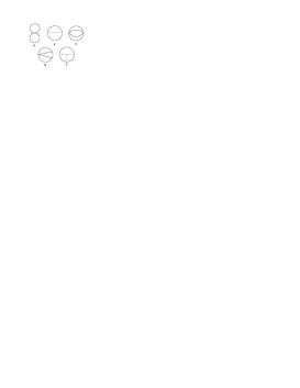
Figure 1: 2PI vacuum diagrams contributing to $\Gamma^{2}(\varphi,G)$ up to the three loop level.

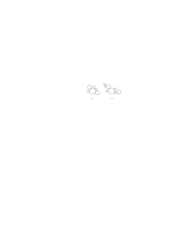
Figure 2: Examples of bubble diagrams.

Using (8) the gap equation (5) may be rewritten in the form

$$G^{-1}(x,y)=D^{-1}(x,y)+2\frac{\delta\Gamma^{2}(\varphi,G)}{\delta G(x,y)}.$$ (9)

One can also recover the usual 1PI-effective action $\Gamma(\varphi)$ simply evaluating $\Gamma[\varphi,G]$ at nonvanishing $J(x)$ but at vanishing $K(x,y)$:

$$\Gamma_{1PI}(\varphi)=\Gamma[\varphi,G_{0}],$$ (10)

where $G_{0}$ is solution of the gap equation (5).

As usual, if one is interested in the vacuum state of the theory (and the vacuum state preserves translational invariance), it is possible to adopt, in place of the effective action (10), the simpler effective potential $V(\varphi)$ defined by

$$\Gamma[\varphi,G_{0}]\equiv-\int dx^{4}V(\varphi).$$ (11)

This CJT formalism which at first sight might appear more involved than the standard formalism, with only the source $J$ coupled to the field, turns out to be very useful in the so-called bubble resummation, which takes into account all the vacuum to vacuum diagrams of the type of Fig.2. In the CJT formalism one obtains the whole bubble resummation [28] simply considering the “eight”-diagram ($A$ in Fig.1) contribution to $\Gamma^{2}(\varphi,G)$. We will use this approximation, also known as Hartree-Fock approximation, in the following sections.

3 CJT formalism in noncommutative field theories

Having outlined the basic features of the CJT formalism we can proceed to apply it to the noncommutative $\lambda\varphi^{4}$ scalar theory. We recall [8] that the action is given by

$$S=\int dx^{4}\left\{\frac{1}{2}m^{2}\phi^{2}+\frac{1}{2}\partial_{\mu}\phi\partial^{\mu}\phi+\frac{\lambda}{4!}\phi\star\phi\star\phi\star\phi\right\},$$ (12)

where $\star$ represents the Moyal product:

$$\varphi_{1}(x)\star\varphi_{2}(x)=\varphi_{1}(x)e^{\frac{i}{2}\theta^{\mu\nu}\overleftarrow{\partial}_{\mu}\overrightarrow{\partial}_{\nu}}\varphi_{2}(x),$$ (13)

with $\theta^{\mu\nu}$ coordinate-independent antisymmetric matrix.

In terms od the Moyal $\star$-product (13) the quadratic part of the action remains unaffected by noncommutativity, while a $\theta$-dependence arises for the interaction term. No specific assumptions are made in the CJT formalism about the form of the interaction therefore procedure outlined in Section-2 (and in particular Eq.(8)) is still valid in this noncommutative context.

It is easily seen that in the case under consideration:

$$D^{-1}(x,y) =\frac{\delta^{2}S}{\delta\varphi(x)\delta\varphi(y)}=$$ (14)

$$=-\left[\square+m^{2}\right]_{x}\delta^{4}(x-y)-\frac{\lambda}{3!}\left\{\delta^{4}(x-y)\star\varphi\star\varphi+\varphi\star\delta^{4}(x-y)\star\varphi+\varphi\star\varphi\star\delta^{4}(x-y)\right\},$$

$$D_{0}^{-1}(x,y) =D^{-1}|_{\lambda=0}=-\left[\square+m^{2}\right]_{x}\delta^{4}(x-y).$$ (15)

As expected $D_{0}^{-1}(x,y)$ is not modified by noncommutativity since the integrals of terms quadratic in the fields are not modified by the $\star$-product (13), while $D^{-1}(x,y)$ acquires the $\theta$-dependence. The $\star$-products which appear in (14) can be easily calculated in momentum space.

Next let us consider the $S_{int}$ action. One can proceed in two steps. The first step is the translation of the action $S(\phi)\rightarrow S(\phi+\varphi)$. The second step is the one of retaining from the shifted action only cubic, and higher, terms in $\phi.$ So doing one obtains

$$S_{int}(\phi;\varphi)=\frac{\lambda}{4!}\int dx^{4}\phi\star\phi\star\phi\star\phi+\frac{\lambda}{6}\int dx^{4}\phi\star\phi\star\phi\star\varphi,$$

where the cyclicity of the $\star$-product (13) under integration has been used.

To proceed further we now need to adopt an ansatz for the form of $G(x,y).$ Since we intend to obtain the CJT effective potential we must assume translational invariance, so that the more general ansatz we can consider takes the form

$$G(x,y)=G(x-y)=\int\frac{d\alpha^{4}}{(2\pi)^{4}}\frac{\exp i\alpha(x-y)}{\alpha^{2}+M^{2}(\alpha)}$$ (16)

where $M^{2}(\alpha)$ is to be determined. Once the ansatz (16) has been done we can calculate the various terms in the left-hand-side of (8). The result is

$$\Gamma(\varphi,G) =\frac{1}{2}\int dx^{4}\left\{(\partial_{\mu}\varphi)^{2}+m^{2}\varphi^{2}\right\}+\frac{\lambda}{4!}\int dx^{4}\varphi\star\varphi\star\varphi\star\varphi+$$ (17)

$$+\frac{1}{2}\int dx^{4}\int\frac{dp^{4}}{(2\pi)^{4}}\ln\left\{\frac{p^{2}+M^{2}(p)}{p^{2}+m^{2}}\right\}+$$

$$+\frac{1}{2}\int dx^{4}\int\frac{dk^{4}}{(2\pi)^{4}}\frac{m^{2}-M^{2}(k)+\dfrac{\lambda}{3!}\int\frac{dp_{1}^{4}dp_{2}^{4}}{(2\pi)^{8}}F(p_{1},p_{2},k)\exp ix(p_{1}+p_{2})\widetilde{\varphi}(p_{1})\widetilde{\varphi}(p_{2})}{k^{2}+M^{2}(k)}+$$

$$+\Gamma^{2}(\varphi,G)$$

where $\widetilde{\varphi}(p)$ is the Fourier transform of $\varphi(x)$. $F(p_{1},p_{2},k)$, using the notation $p_{i}\theta p_{j}\equiv p_{i}^{\mu}\theta_{\mu\nu}p_{j}^{\nu}$, takes the form

$$F(p_{1},p_{2},k) =\exp-\frac{i}{2}\left(p_{1}\theta p_{2}+k\theta p_{1}+k\theta p_{2}\right)+$$

$$+\exp-\frac{i}{2}\left(p_{1}\theta k+p_{1}\theta p_{2}+k\theta p_{2}\right)+$$

$$+\exp-\frac{i}{2}\left(p_{1}\theta p_{2}+p_{1}\theta k+p_{2}\theta k\right).$$ (18)

The first row in (17) is just $S(\varphi)$, the second row is $Tr\ln(D_{0}^{-1}G)$, the third is $Tr\left\{D^{-1}G-1\right\}$.

Now we must evaluate $\Gamma^{2}(\varphi,G)$ with vertices given by $S_{int}(\phi;\varphi)$ and propagator given by $G(x,y).$ As a first application of the formalism one can recover the usual one-loop 1PI effective action [8] simply setting $\Gamma^{2}=0$. In this case the gap equation (9) trivially reduces to

$$G^{-1}(x,y)=D^{-1}(x,y),$$ (19)

and (8) becomes

$$\Gamma(\varphi)=S(\varphi)+\frac{1}{2}Tr\ln D^{-1}(\varphi)D_{0}.$$

That is just the one-loop 1PI effective action.

While neglecting $\Gamma^{2}$ completely gives us back the one-loop 1PI effective action, a more interesting result is obtained by approximating $\Gamma^{2}(\varphi,G)$ including only the “eight” diagram (A in Fig.1). In this approximation one has that

$$\Gamma^{2}(\varphi,G)=\frac{1}{4!}\lambda\delta^{4}(0)\int\frac{d\alpha^{4}d\alpha^{\prime 4}}{(2\pi)^{8}}\frac{1}{\alpha^{2}+M^{2}(\alpha)}\frac{1}{\alpha^{\prime 2}+M^{2}(\alpha^{\prime})}\left\{1+2\cos^{2}(\frac{\alpha\theta\alpha^{\prime}}{2})\right\}.$$ (20)

We observe that differently from the commutative case, where the momenta circulating in each of the two loops do not mix (so that $\Gamma^{2}$ is evaluated as the products of two single-variable integrals), in the commutative case this mixing occurs.

4 The CJT effective potential in noncommutative field theories

From the effective action (17) and (20), assuming translational invariance of the candidate vacua $\varphi(x)=\varphi$, one can extract the effective potential (11):

$$V(\varphi) =\frac{1}{2}m^{2}\varphi^{2}+\frac{\lambda}{4!}\varphi^{4}+$$ (21)

$$+\frac{1}{2}\int\frac{dp^{4}}{(2\pi)^{4}}\ln\left\{\frac{p^{2}+M^{2}(p)}{p^{2}+m^{2}}\right\}+$$

$$+\frac{1}{2}\int\frac{dk^{4}}{(2\pi)^{4}}\frac{m^{2}-M^{2}(k)+\dfrac{\lambda}{2}\varphi^{2}}{k^{2}+M^{2}(k)}+$$

$$+\frac{1}{4!}\lambda\int\frac{d\alpha^{4}d\alpha^{\prime 4}}{(2\pi)^{8}}\frac{1}{\alpha^{2}+M^{2}(\alpha)}\frac{1}{\alpha^{\prime 2}+M^{2}(\alpha^{\prime})}\left\{2+\cos(\alpha\theta\alpha^{\prime})\right\}.$$

The stationarity condition (5) in this case becomes $\frac{\partial V(\varphi)}{\partial\varphi}=0$ which implies the gap equation

$$M^{2}(\alpha)-m^{2}-\dfrac{\lambda}{2}\varphi^{2}-\frac{\lambda}{6}\int\frac{db^{4}}{(2\pi)^{4}}\frac{2+\cos\left(b\theta\alpha\right)}{b^{2}+M^{2}(b)}=0.$$ (22)

Substituting equation (22) in the expression of the potential (21) we obtain

$$V(\varphi,G) =\frac{1}{2}m^{2}\varphi^{2}+\frac{\lambda}{4!}\varphi^{4}+\frac{1}{2}\int\frac{dp^{4}}{(2\pi)^{4}}\ln\left\{\frac{p^{2}+M^{2}(p)}{p^{2}+m^{2}}\right\}+$$ (23)

$$-\frac{\lambda}{24}\int\frac{dk^{4}}{(2\pi)^{4}}\frac{1}{k^{2}+M^{2}(k)}\int\frac{db^{4}}{(2\pi)^{4}}\frac{1}{b^{2}+M^{2}(b)}\left\{2+\cos\left(b\theta k\right)\right\}.$$

The term in the second row of the above expression is generated by the bubble summation. The terms appearing in the first row are already present at one-loop level but what is different here is that they now must be evaluated for $M^{2}(p)$ solution of the gap equation (22) which involves a non-trivial $\theta$-dependence. Clearly our CJT resummed effective potential has complicated $\theta$-dependence whereas the 1-loop effective potential is completely $\theta$-independent. We notice that $\theta$-dependence manifests in two different ways: the tree-level and the one-loop like contributions depend on $\theta$ only through $M^{2}(p)$ whereas the term generated by the bubble summation (the last one in (23)) also exhibits an explicit $\theta$-dependence.

Both (22) and (23) are ultraviolet divergent and they both are considered to be regularized with a cutoff $\Lambda$ on the loop-momenta. In the next section we will deal with the problem of their renormalization but first we recall the strategy of renormalization adopted in the commutative case ($\theta=0$).

4.1 Renormalization of the effective potential for $\theta=0$

In the commutative case (22) and (23) become respectively

$$M^{2}(\alpha)=m^{2}+\dfrac{\lambda}{2}\varphi^{2}+\frac{\lambda}{2}\int\frac{db^{4}}{(2\pi)^{4}}\frac{1}{b^{2}+M^{2}(b)}$$ (24)

and

$$V(\varphi,G)=\frac{1}{2}m^{2}\varphi^{2}+\frac{\lambda}{4!}\varphi^{4}+\frac{1}{2}\int\frac{dp^{4}}{(2\pi)^{4}}\ln\left\{\frac{p^{2}+M^{2}(p)}{p^{2}+m^{2}}\right\}-\frac{\lambda}{8}\int\frac{dk^{4}}{(2\pi)^{4}}\frac{1}{k^{2}+M^{2}(k)}\int\frac{db^{4}}{(2\pi)^{4}}\frac{1}{b^{2}+M^{2}(b)}.$$ (25)

We immediately see, from Eq.(24), that in this case $M^{2}(\alpha)$ does not depend on the loop-momentum $\alpha$ so that one can set $M^{2}(\alpha)\equiv M^{2}$ both in (24) and in (25).

Renormalization of the effective potential for $\theta=0$ is a well-known result (see e.g. [30]). We recall the procedure that one can use to renormalize (24) and (25) since we will use it widely in the rest of the paper. In order to renormalize this gap equation (24) it is convenient to introduce $I_{1},I_{2},G_{R}$ through the formula

$$\int\frac{db^{4}}{(2\pi)^{4}}\frac{1}{b^{2}+M^{2}}=I_{1}-I_{2}M^{2}+G_{R}(M),$$ (26)

where

$$I_{1} =\int\frac{db^{4}}{(2\pi)^{4}}\frac{1}{b^{2}},$$ (27)

$$I_{2} =\int\frac{db^{4}}{(2\pi)^{4}}\frac{1}{b^{4}},$$ (28)

and $G_{R}(M)$ is the finite part of $G(M)$. The gap equation can then be rewritten in the form

$$M^{2}\left(\frac{1}{\lambda}+\frac{1}{2}I_{2}\right)=\frac{m^{2}}{\lambda}+\frac{1}{2}I_{1}+\frac{1}{2}\varphi^{2}+\frac{1}{3}G_{R}(M).$$ (29)

Introducing the renormalized parameters

$$\dfrac{1}{\lambda_{R}} =\lim_{\Lambda\rightarrow\infty}\left[\frac{1}{\lambda}+\frac{1}{2}I_{1}\right],$$ (30)

$$\dfrac{m_{R}^{2}}{\lambda_{R}} =\lim_{\Lambda\rightarrow\infty}\left[\frac{m^{2}}{\lambda}+\frac{1}{2}I_{2}\right],$$ (31)

one gets the renormalized gap equation

$$M^{2}=m_{R}^{2}+\dfrac{\lambda_{R}}{2}\varphi^{2}+\frac{\lambda_{R}}{3}G_{R}(M).$$

Next one verifies that the conditions (30) and (31) also renormalize the effective potential. For this objective one observes that using (24) one can write (25) as the sum of three contributions

$$V^{0} =\frac{1}{2}m^{2}\varphi^{2}+\frac{\lambda}{4!}\varphi^{4},$$ (32)

$$V^{I} =\frac{1}{2}\int\frac{dk^{4}}{(2\pi)^{4}}\ln(k^{2})+\frac{1}{2}I_{1}M^{2}-\frac{1}{4}I_{2}M^{4}+T(M)$$ (33)

$$V^{II} =-\frac{1}{2}GM^{2}+\frac{1}{2\lambda}M^{4}-\frac{1}{2\lambda}m^{4}-\frac{1}{2}m^{2}\varphi^{2}-\frac{\lambda}{8}\varphi^{4},$$ (34)

that gives

$$V=V^{II}+V^{I}+V^{0}=-\frac{\lambda}{12}\varphi^{4}+\frac{1}{2}\frac{M^{4}}{\lambda_{R}}-\frac{1}{2}M^{2}G_{R}(M)+T(M),$$ (35)

where $T(M)$ is a finite contribution to $V^{I}$ (which of course is not significant for renormalizability) and the field-independent terms have been discarded.

We observe that the CJT effective potential (35) in terms of the renormalized parameters, defined by (30) and (31), is finite. One could be concerned with the unrenormalized contribution $-\frac{\lambda}{12}\varphi^{4}$ but since from Eq.(30) it follows that $\lambda(\Lambda)\simeq(\lambda_{R}-\frac{1}{2}I_{2})^{-1}$ the term $-\frac{\lambda}{12}\varphi^{4}$ vanishes upon removal of the cutoff.

In preparation for a key observation made in the following section let us also emphasize the exact cancellation of the potentially dangerous divergent terms of type $m^{2}\varphi^{2}$ which appear with opposite signs in the tree level contribution $V^{0}$ and in the loop correction $V^{II}$.

4.2 Renormalization of the effective potential for $\theta\neq 0$

Now we want to address the problem of evaluating the effective potential for nonvanishing values of the noncommutativity parameter $\theta$. In the analysis of the gap equation (22) one finds immediately an important complication due to nonvanishing $\theta$. In fact a constant $M^{2}$ clearly cannot be a solution of (22) and the gap equation must then be solved for a momentum-dependent function $M^{2}(p)$.

We start by defining $M^{2}(\alpha)=M^{2}+\Pi(\alpha)$ so that the gap equation (22) can be rewritten as

$$\Pi(\alpha)=-M^{2}+m^{2}+\dfrac{\lambda}{2}\varphi^{2}+\frac{\lambda}{3}\int\frac{db^{4}}{(2\pi)^{4}}\frac{1}{b^{2}+M^{2}+\Pi(b)}+\frac{\lambda}{6}\int\frac{db^{4}}{(2\pi)^{4}}\frac{\cos\left(b\theta\alpha\right)}{b^{2}+M^{2}+\Pi(b)}.$$

We use the freedom in the choice of the “constant” part of $M^{2}(\alpha)$ to make it satisfy

$$M^{2}=m^{2}+\dfrac{\lambda}{2}\varphi^{2}+\frac{\lambda}{3}\int\frac{db^{4}}{(2\pi)^{4}}\frac{1}{b^{2}+M^{2}+\Pi(b)},$$ (36)

and

$$\Pi(\alpha)=\frac{\lambda}{6}\int\frac{db^{4}}{(2\pi)^{4}}\frac{\cos\left(b\theta\alpha\right)}{b^{2}+M^{2}+\Pi(b)}.$$ (37)

We notice that the integral in the right-hand-side of Eq.(37) is finite both in the ultraviolet sector and in the infrared sector so that Eq.(37) does not need to be renormalized. We also observe that $\Pi(\alpha)\rightarrow\infty$ for $\alpha\rightarrow 0$ and for $\theta\rightarrow 0$, and that $\Pi(\alpha)\rightarrow 0$ for $\alpha\rightarrow\infty$ and for $\theta\rightarrow\infty$.

Equation (36), on the contrary, is not UV-finite. It can be renormalized by a procedure similar to the one we have discussed previously. Introducing the renormalized parameters in the form

$$\dfrac{1}{\lambda_{R}} =\lim_{\Lambda\rightarrow\infty}\left[\frac{1}{\lambda}+\frac{1}{3}I_{2}\right],$$ (38)

$$\dfrac{m_{R}^{2}}{\lambda_{R}} =\lim_{\Lambda\rightarrow\infty}\left[\frac{m^{2}}{\lambda}+\frac{1}{3}I_{1}\right],$$ (39)

we get the renormalized gap equation

$$M^{2}=m_{R}^{2}+\dfrac{\lambda_{R}}{2}\varphi^{2}+\frac{\lambda_{R}}{3}F_{R}(M),$$

where $F_{R}(M)$ is the finite part of the divergent integral in (36):

$$F_{R}(M)=\int\frac{db^{4}}{(2\pi)^{4}}\frac{1}{b^{2}+M^{2}+\Pi(b)}-\left[\int\frac{db^{4}}{(2\pi)^{4}}\frac{1}{b^{2}}-M^{2}\int\frac{db^{4}}{(2\pi)^{4}}\frac{1}{b^{4}}\right]$$ (40)

We come now to the important issue of the renormalization of the effective potential. We have seen that the way in which the gap equation renormalizes fixes uniquely the renormalization of the bare mass and the renormalization of the coupling. We must check if the same renormalization conditions provide us a finite effective potential. We can use (36) and (37) in the expression (23) to obtain the effective potential as the sum of the three following terms:

$$V^{0} =\frac{1}{2}m^{2}\varphi^{2}+\frac{\lambda}{4!}\varphi^{4},$$ (41)

$$V^{I} =\frac{1}{2}\int\frac{dk^{4}}{(2\pi)^{4}}\ln(k^{2})+\frac{1}{2}I_{1}M^{2}-\frac{1}{4}I_{2}M^{4}+T(M,\Pi),$$ (42)

$$V^{II} =M^{4}\left\{\frac{1}{2}I_{2}+\dfrac{3}{4}\dfrac{1}{\lambda}\right\}+\frac{M^{2}}{2}\int\frac{dk^{4}}{(2\pi)^{4}}\frac{\Pi(k)[\Pi(k)+2k^{2}]}{k^{4}\left[k^{2}+\Pi(k)\right]^{2}}$$

$$+M^{2}\left\{-\dfrac{1}{2}I_{1}-\dfrac{1}{2}\int\frac{dk^{4}}{(2\pi)^{4}}R(k)+\dfrac{1}{4}\int\frac{dk^{4}}{(2\pi)^{4}}\frac{\Pi(k)}{k^{2}+\Pi(k)}\left(\frac{1}{k^{2}+\Pi(k)}+\frac{2}{k^{2}}\right)\right\}+$$

$$-\dfrac{1}{4}\int\frac{dk^{4}}{(2\pi)^{4}}\frac{\Pi(k)}{k^{2}+\Pi(k)}-\dfrac{1}{4}\int\frac{dk^{4}}{(2\pi)^{4}}\Pi(k)R(k)-\dfrac{3m^{4}}{4\lambda}-\dfrac{3}{4}m^{2}\varphi^{2}-\dfrac{3}{16}\lambda\varphi^{4},$$ (43)

where we have defined

$$T(M,\Pi)=\dfrac{1}{2}\int\frac{dk^{4}}{(2\pi)^{4}}\ln[k^{2}+M^{2}+\Pi(k)]-\left\{\dfrac{1}{2}\int\frac{dk^{4}}{(2\pi)^{4}}\ln[k^{2}]+\frac{M^{2}}{2}\int\frac{dk^{4}}{(2\pi)^{4}}\frac{1}{k^{2}}-\frac{M^{4}}{4}\int\frac{dk^{4}}{(2\pi)^{4}}\frac{1}{k^{4}}\right\},$$

and

$$R(k)=\tfrac{1}{k^{2}+M^{2}+\Pi(k)}-\left\{\tfrac{1}{k^{2}+\Pi(k)}-\tfrac{M^{2}}{\left[k^{2}+\Pi(k)\right]^{2}}\right\}.$$ (44)

We observe that in our CJT effective potential ($V=V^{0}+V^{I}+V^{II}$), thanks to the fact that $\Pi(k)$ vanishes exponentially in the limit $k\rightarrow\infty$, all the field-dependent terms, with the exception of $m^{2}\varphi^{2}$ and $\lambda\varphi^{4}$ terms, are cutoff independent. The term in $\lambda\varphi^{4}$ is not divergent, it is similar to the $\lambda\varphi^{4}$-term present in the commutative case and can be handled in the same way. The term in $m^{2}\varphi^{2}$, on the contrary, is genuinely ultraviolet divergent. This is due to the fact that the corresponding contributions from $V^{0}$ and $V^{II}$ do not cancel each other (unlike the commutative case). This clearly originates from the well-known fact that nonvanishing $\theta$, by regularizing certain otherwise divergent diagrams, effectively changes the numerical coefficients in front of some divergent terms.

The presence of this $\varphi$-dependent contribution that diverges upon cutoff removal leads to conjecture that it is impossible for this theory to be in an ordered translationally invariant phase.

4.3 Renormalization of the effective potential in the planar limit ($\theta\rightarrow\infty$)

It is also interesting to consider the limit of strong noncommutativity ($\theta\rightarrow\infty$). In this limit the strong oscillations in the phases, which are present in the integrands of (22) and (23), induce the vanishing of the corresponding integrals. In this limit the nonplanar contribution of the eight diagram becomes negligible and only the planar contribution survives. In this strong commutativity limit the effective potential is given by the sum of the terms

$$V^{0} =\frac{1}{2}m^{2}\varphi^{2}+\frac{\lambda}{4!}\varphi^{4},$$ (45)

$$V^{I} =\frac{1}{2}\int\frac{dk^{4}}{(2\pi)^{4}}\ln(k^{2})+\frac{1}{2}I_{1}M^{2}-\frac{1}{4}I_{2}M^{4}+T(M,0),$$ (46)

$$V^{II} =-\frac{3}{4\lambda}m^{4}-\dfrac{3\lambda}{16}\varphi^{4}+\frac{3}{4\lambda}M^{4}-\dfrac{1}{2}M^{2}G(M)-\frac{3}{4}m^{2}\varphi^{2},$$ (47)

so that one finds

$$\ V=\frac{3}{4}\frac{M^{4}}{\lambda_{R}}-\frac{7}{48}\lambda\varphi^{4}-\frac{1}{4}m^{2}\varphi^{2}-\dfrac{1}{2}M^{2}G_{R}(M)+T(M,0).$$ (48)

This expressions for the effective potential is formally similar to the ones of the commutative case, (35). The crucial differences consist in the factors in front to the eight-diagram terms. It particular in this limit, as in the commutative case, the dressed mass $M^{2}(k)=M^{2}+\Pi(k)$ becomes momentum independent since $\Pi(k)$ vanishes exponentially.

Again the cancellation between the $m^{2}\varphi^{2}$ terms in (45) and (47) doesn’t occur and the resulting potential doesn’t renormalize.

5 Conclusions

Whereas in commutative spacetime the CJT effective potential can be renormalized and gives a satisfactory description of the vacua of a given field theory, in our canonical-noncommutativity analysis the CJT effective potential (in the bubble-resummation approximation) was found not to be renormalizable. From a conservative standpoint we should then assume that in this type of theories the CJT effective potential cannot provide reliable nonperturbative insight on the phase structure. This negative conclusion is also supported by the realization that canonical noncommutativity affects strongly the structure of the UV divergences of a field theory, and this might be particularly significant for those techniques that effectively rely on resummations of contributions from all orders in the coupling constant. When we establish that a field theory is renormalizable, we actually verify that it is “perturbatively renormalizable”: the divergences at any given order in coupling-expansion perturbation theory can be reabsorbed in redefinitions of the parameters of the Lagrangian density. The fact that the CJT technique gives rise to a renormalizable effective potential in the commutative-spacetime case is highly nontrivial, since we are not consistently summing all contributions up to a given order in the coupling constant (a calculation which would be “protected” by perturbative renormalizability), we are instead selectively summing a certain subset of the contributions at all orders in the coupling constant. It is therefore plausible that the fact that our CJT effective potential cannot be renormalized is simply a sign of an inadequacy of this technique to the canonical-noncommutativity context.

On the other hand it appears reasonable to explore an alternative, more optimistic, perspective, which is based on the observation that the only contribution to the CJT potential that ends up not being expressed in terms of renormalized quantities is the $\frac{1}{4}m^{2}\varphi^{2}$ contribution. This term however will vanish in a disordered phase $\varphi=0$. In a certain sense we have a renormalizable effective potential in the disordered phase, and our results of nonrenormalizability in the translationally-invariant ordered phase $\varphi=C$ could be interpreted as a manifestation of the fact that this phase is not admissable for these theories in canonical noncommutative spacetime. This hypothesis finds some support in the arguments presented in Ref. [19], which also concluded that the only admissible phases for these theories are the disordered phase and a (non-translationally-invariant) stripe phase with $\tilde{\varphi}(p)=C\delta(p-p_{c})$ (where $\tilde{\varphi}(p)$ is the Fourier transform of $\varphi(x)$) and $p_{c}$ is a characteristic momentum scale of the stripe phase). This argument of inadmissability of the translationally-invariant ordered phase might be related with the delicate IR structure of these theories: $\varphi(x)=C$ means $\tilde{\varphi}(p)=C\delta(p)$, so the concept of a translationally-invariant ordered phase is closely connected with the zero-momentum structure of the theory of interest.

The fact that various lines of analysis appear to suggest that a non-translationally-invariant ordered phase should naturally be considered in these theories is rather intriguing. In fact canonical noncommutativity is naturally in conflict with invariance under space rotations and/or boosts, but, when analyzed as a pure algebra of coordinates, appears to be perfectly compatible with classical translational invariance. If a non translational invariant ordered phase emerges from field theories in canonical noncommutative spacetime it would mean that these theories might favour spontaneous breaking of their only residual spacetime symmetry (the one under spacetime translations).

To explore these issues it would be necessary to consider the CJT effective action, which explores the more general class of candidate vacua $\varphi(x)$, rather than stopping, as we did here, at the level of the CJT effective potential (which assumes from the beginning a translationally-invariant vacuum). With the CJT effective action one could investigate the renormalizability of the stripe phase (which is not translationally invariant, and therefore cannot be studied with the effective potential). Unfortunately even in commutative-spacetime theories the evaluation of the CJT effective action turns out to be very complex (basically intractable analytically and a troublesome calculation even numerically). It is likely that in the canonical-noncommutativity context the evaluation of the CJT effective action may prove even more troublesome, but from the indications that emerged from our analysis of the CJT effective potential it appears that such an analysis is well motivated, as it could provide insight for the understanding of some key physical predictions of these theories.

Note added

These results were first presented in Chapter 5, of my Ph.D. thesis [39]. As I was rewriting the discussion in a format more suitable for the article-style presentation here provided the study in Ref.[40] was announced. The results reported in Ref.[40] are consistent (and partially overlap) with the ones presented here and in Ref.[39].

References

- [1] S. Doplicher, K. Fredenhagen, J.E. Roberts, The quantum structure of space-time at the Planck scale and quantum fields, Commun. Math. Phys. 172 (1995) 187-220, hep-th/0303037.
- [2] T. Filk, Divergencies in a field theory on quantum space, Phys. Lett. B376 (1996) 53.
- [3] M.R. Douglas, N.A. Nekrasov, Noncommutative field theory, Rev. Mod. Phys. (2001) 977-1029, hep-th/0106048.
- [4] R.J. Szabo, Quantum field theory on noncommutative spaces, hep-th/0109162.
- [5] A. Connes, M. R. Douglas, A. Schwarz, Noncommutative Geometry and Matrix Theory: Compactification on Tori, JHEP 9802 (1998) 003, hep-th/9711162.
- [6] N. Seiberg, E. Witten, String theory and noncommutative geometry, JHEP 09 (1999) 032, hep-th/9908142.
- [7] I.Y. Arefeva, D.M. Belov, A.A. Giryavets, A.S. Koshelev, P.B. Medvedev, Noncommutative field theories and (super)string field theories, Campos do Jordao 2001, Particles and fields, 1-163, hep-th/0111208.
- [8] S. Minwalla, M. Van Raamsdonk, N. Seiberg, Noncommutative perturbative dynamics, JHEP 02 (2000) 020, hep-th/9912072.
- [9] M. Van Raamsdonk, N. Seiberg, Comments on noncommutative perturbative dynamics, JHEP 0003 (2000) 035, hep-th/0002186.
- [10] A. Matusis, L. Susskind, N. Toumbas, The IR/UV connection in the noncommutative gauge theories, JHEP 0012 (2000) 002, hep-th/0002075.
- [11] G. Amelino-Camelia, L. Doplicher, S. Nam, Y. Seo, Phenomenology of Particle Production and Propagation in String-Motivated Canonical Noncommutative Spacetime, hep-th/0109191.
- [12] G. Amelino-Camelia, M. Arzano, L. Doplicher, Field theories on canonical and Lie-algebra noncommutative spacetimes, hep-th/0205047.
- [13] G. Amelino-Camelia, G. Mandanici, K.Yoshida, On the IR / UV mixing and experimental limits on the parameters of canonical noncommutative spacetimes, hep-th/0209254.
- [14] I. Ya. Aref’eva, D.M. Belov, A.S. Koshelev, Two-Loop Diagrams in Noncommutative theory, Phys.Lett. B476 (2000) 431-436, hep-th/9912075.
- [15] A. Micu, M.M. Sheikh-Jabbari, Noncommutative Theory at Two Loops, JHEP 0101 (2001) 025, hep-th/0008057.
- [16] L. Griguolo, M. Pietroni, Wilsonian Renormalization Group and the Non-Commutative IR/UV Connection, JHEP 0105 (2001) 032, hep-th/0104217.
- [17] J. Polchinski, Renormalizations and effective lagrangians, Nucl. Phys. B231 (1984) 269-295.
- [18] S. Sarkar, On the UV renormalizability of noncommutative field theories, JHEP 0206 (2002) 003, hep-th/0202171.
- [19] S.S. Gubser, S.L. Sondhi, Phase structure of non-commutative scalar field theories, Nucl.Phys. B605 (2001) 395-424, hep-th/0006119.
- [20] W. Bietenholz, F. Hofheinz, J. Nishimura, Simulating non-commutative field theory, hep-lat/0209021.
- [21] J. Ambjorn, S. Catterall, Stripes from (noncommutative) stars, hep-lat/0209106.
- [22] W. Bietenholz, F. Hofheinz, J. Nishimura, Non–commutative field theories beyond perturbation theory, hep-th/0212258.
- [23] B. A. Campbell, K. Kaminsky, Noncommutative field theory and spontaneous symmetry breaking, Nucl.Phys. B581 (2000) 240-256, hep-th/0003137.
- [24] E.T. Akhmedov, P. DeBoer, G.W. Semenoff, Non-commutative Gross-Neveu model at large N, JHEP 0106 (2001) 009, hep-th/0103199.
- [25] F. Ruiz Ruiz, UV/IR mixing and the Goldstone theorem in noncommutative field theory, Nucl.Phys. B637 (2002) 143-167, hep-th/0202011.
- [26] S. Sarkar, B. Sathiapalan Comments on the renormalizability of the broken symmetry phase in noncommutative scalar field theory, JHEP 0105 (2001) 049, hep-th/0104106.
- [27] H.O. Girotti, M. Gomes, A.Yu. Petrov, V.O. Rivelles, A.J. da Silva, Spontaneous symmetry breaking in noncommutative field theory, hep-th/0207220.
- [28] J.M. Cornwall, R. Jackiw, E. Tomboulis, Effective action for composite operators, Phys.Rev.D10 (1974) 2428-2445.
- [29] R. Jackiw, G. Amelino-Camelia, Field Theoretical Background for Thermal Physics, Proceedings of the III Workshop on Thermal Field Theories and Their Applications, Banff, Canada, August 15-27, 1993, hep-ph/9311324.
- [30] G. Amelino-Camelia, S.-Y. Pi, Self-consistent Improvement of the Finite Temperature Effective Potential, Phys.Rev. D47 (1993) 2356-2362, hep-ph/9211211.
- [31] G. Amelino-Camelia, Self-consistently Improved Finite Temperature Effective Potential for Gauge Theories, Phys.Rev. D49 (1994) 2740-2751, hep-ph/9305222.
- [32] G. Amelino-Camelia, On the CJT formalism in multifield theories, Nucl.Phys. B476 (1996) 255-274, hep-ph/9305222.
- [33] C. Aragão de Carvalho, S. Caracciolo and J. Fröhlich, Polymers and g theory in four dimensions, Nucl. Phys. B215 (1983) 209, and references therein.
- [34] S.Majid, H. Ruegg, Bicrossproduct structure of kappa poincare group and noncommutative geometry, Phys.Lett. B334 (1994) 348-354, hep-th/9405107.
- [35] J. Lukierski, H. Ruegg, W.J. Zakrzewski, Classical quantum mechanics of free kappa relativistic systems, Annals Phys. 243 (1995) 90-116, hep-th/9312153.
- [36] G. Amelino-Camelia, S. Majid, Waves on noncommutative space-time and gamma-ray bursts, Int.J.Mod.Phys. A15 (2000) 4301-4324, hep-th/9907110.
- [37] G. Amelino-Camelia, Relativity in space-times with short distance structure governed by an observer independent (Planckian) length scale, Int.J.Mod.Phys. D11 (2002) 35-60, gr-qc/0012051.
- [38] N.R. Bruno, G. Amelino-Camelia, J. Kowalski-Glikman, Deformed boost transformations that saturate at the Planck scale, Phys.Lett. B522 (2001) 133-138, hep-th/0107039.
- [39] G. Mandanici, Wave propagation and IR/UV mixing in noncommutative spacetimes, Ph.D. Thesis, University of Roma “La Sapienza”, December 2002, Roma, Italy.
- [40] P. Castorina, D. Zappalà, Nonuniform symmetry breaking in noncommutative theory, hep-th/0303030.