Torsion and nonmetricity in the stringy geometry

Abstract:

In the present article, we study the space-time geometry felt by probe bosonic string moving in antisymmetric and dilaton background fields. This space-time geometry we shall call the stringy geometry. In particular, the presence of the antisymmetric field leads to the space-time torsion, and the presence of the dilaton field leads to the space-time nonmetricity. We generalize the geometry of surfaces embedded in space-time to the case when torsion and nonmetricity are present. We define the mean extrinsic curvature for Minkowski signature and introduce the concept of mean torsion. Its orthogonal projection defines the dual mean extrinsic curvature. In this language, one field equation is just the equality of mean extrinsic curvature and dual mean extrinsic curvature, which we call C-duality relation. In the torsion and nonmetricity free case, the world-sheet is a minimal surface, specified by the requirement that mean extrinsic curvature vanishes. Generally, it is stringy C-dual surface. In the presence of the dilaton field, which breaks conformal invariance, the conformal factor which connects intrinsic and induced metrics, is determined as a function of the dilaton field itself. We also derive the integration measure for the space-time with stringy nonmetricity.

1 Introduction

In the paper [1], we investigated classical dynamics of the bosonic string in the background metric, antisymmetric and dilaton fields. The starting Lagrangian has been used in the literature [3, 4, 5], in order to study the two-dimensional conformal invariance on the quantum level. In those papers the classical space-time equations of motion have been obtained from the world-sheet quantum conformal invariance.

In the ref. [1], we made classical canonical nonperturbative investigations, treating world-sheet fields as variables in the theory and space-time fields as a background depending on the coordinates $x^{\mu}$. We obtained the nonlinear realization of the Virasoro generators. We also derived the Hamiltonian equations of motion and shortly discussed the target space torsion and nonmetricity, recognized by the string.

In the present paper, we are going to investigate in detail the space-time geometry felt by the string, and offer geometrical interpretation of the equations of motion. In Sec. 2, we will consider general theory of surfaces embedded in space-time with torsion and nonmetricity, and in Secs. 3 and 4 we will apply this results to the bosonic string theory in the background fields.

Starting with the known rules of the space-time parallel transport, in Sec. 2 we introduce the torsion and nonmetricity. We decompose the arbitrary connection in terms of the Christoffel one, contortion and nonmetricity. Then we define the induced world-sheet variables: metric tensor and connection, and extrinsic one: second fundamental form (SFF). The world-sheet tangent vector, after parallel transport along world-sheet line with space-time connection is not necessarily a tangent vector. Its world-sheet projection defines the induced connection and its normal projection defines the SFF. When the metric postulate is not valid, there are two forms of the world-sheet connections and two forms of SFF. The two forms, of both the connection and the SFF, differ by terms proportional to the nonmetricity. We also introduce the induced torsion and induced nonmetricity and find the relations between space-time and world-sheet covariant derivatives. We generalized the geometrical interpretation of the SFF to the case where the space-time has nontrivial torsion and nonmetricity. In the standard approach the torsion does not contribute to the mean extrinsic curvature (MEC) ${}^{\circ}H_{i}$. We define dual mean extrinsic curvature (DMEC) ${}^{\ast}H_{i}$ as an orthogonal projection of the mean torsion. This enables us to define the self-dual (self-antidual) condition, under C-duality ${}^{\circ}H_{i}=\pm{}^{\ast}H_{i}$.

In Sec. 3, we formulate the bosonic string theory and shortly repeat some results of ref. [1], such as canonical derivation of the equations of motion. We independently derive the Lagrangian equations of motion and connect them to the previous ones. We introduce the stringy space-time felt by the probe string and find the expressions for stringy torsion and stringy nonmetricity.

In Sec. 4, we investigate contributions of the background fields to the space-time geometry. The equations of motion with respect to the intrinsic world-sheet metric relate this intrinsic metric with the induced one. In the absence of the dilaton field $\Phi$, the theory is conformally invariant, so that the intrinsic metric tensor is equal to the induced one up to the conformal factor $\lambda$. The presence of the dilaton field breaks the conformal invariance and determines this conformal factor.

Equations of motion, obtained by variation with respect to $x^{\mu}$, have $D$ components. Two of them determine the contracted intrinsic connection in terms of the corresponding induced expression. The other $D-2$ are of the form ${}^{\star}H_{i}=\pm{}^{\ast}H_{\mp i}$, where ${}^{\star}H_{i}$ is stringy MEC and ${}^{\ast}H_{\pm i}$ are the two forms of DMEC. They define world-sheet as a stringy C-dual (antidual) surface. In two particular cases, —the vanishing torsion and the vanishing nonmetricity— the field equations turn to the equations of stringy minimal world-sheet ${}^{\star}H_{i}=0$ and C-dual (antidual) world-sheet $H_{i}=\pm{}^{\ast}H_{\mp i}$, respectively. In the case of Riemann space-time, when both torsion and nonmetricity vanish, they turn to the equations of minimal world-sheet $H_{i}=0$.

The presence of the space-time metric $G_{\mu\nu}$ produces just the standard Christoffel connection. In this case, the string can see the space-time as Riemannian one. The field strength of the antisymmetric tensor contributes to the space-time torsion. So, string with background fields $G_{\mu\nu}$ and $B_{\mu\nu}$ feels Riemann-Cartan space-time. Finally, the dilaton field $\Phi$ produces the nonmetricity of the space-time. The target space observed by the string, when all three background fields $G_{\mu\nu}$, $B_{\mu\nu}$ and $\Phi$ are present, we will call the stringy space-time.

In sec. 5, we consider the possible forms of the space-time action. We obtain the new integration measure for spaces with nonmetricity from the requirements that the measure is preserved under parallel transport and that it enables integration by parts. We discuss how our action is related to the action of the papers [4, 5].

Appendix A is devoted to the world-sheet geometry, and Appendix B to the classification of space-time geometry and to the world-sheet as an embedded surface.

2 Geometry of surfaces embedded in space-time with torsion and nonmetricity

The geometry of surfaces, when the world-sheet is embedded in curved space-time, has been investigated in the literature, see [6, 7]. In this section we will generalize these results for the space-times with nontrivial torsion and nonmetricity. For some details of the subsection 2.1 see refs. [8, 9].

2.1 Geometry of space-time with torsion and nonmetricity

In the curved spaces, the operations on tensors are covariant only if they are realized in the same point. In order to compare the vectors from different points we need the rule for parallel transport. The parallel transport of the vector $V^{\mu}(x)$, from the point $x$ to the point $x+dx$, produce the vector ${}^{\circ}V^{\mu}_{\parallel}=V^{\mu}+{}^{\circ}\delta V^{\mu}$, where

$${}^{\circ}\delta V^{\mu}=-{}^{\circ}\Gamma_{\rho\sigma}^{\mu}V^{\rho}dx^{\sigma}\,.$$ (1)

The variable ${}^{\circ}\Gamma_{\rho\sigma}^{\mu}$ is the affine linear connection. The rule for the parallel transport of the covector $U_{\mu}(x)$, can be obtained from the requirement that the invariant vector product is not changed under parallel transport ${}^{\circ}\delta(V^{\mu}U_{\mu})=0$, so that

$${}^{\circ}\delta U_{\mu}={}^{\circ}\Gamma_{\mu\nu}^{\rho}U_{\rho}dx^{\nu}\,.$$ (2)

Now, we are able to compare vectors from the points $x$ and $x+dx$, and define the covariant derivative

$${}^{\circ}DV^{\mu}=V^{\mu}(x+dx)-{}^{\circ}V^{\mu}_{\parallel}=dV^{\mu}-{}^{\circ}\delta V^{\mu}=(\partial_{\nu}V^{\mu}+{}^{\circ}\Gamma_{\rho\nu}^{\mu}V^{\rho})dx^{\nu}\equiv{}^{\circ}D_{\nu}V^{\mu}dx^{\nu}\,.$$ (3)

Let us define the geodesic line as a self-parallel line, which means that the tangent vector $t^{\mu}={dx^{\mu}\over ds}=\dot{x}^{\mu}$, stay parallel after parallel transport $\,t^{\mu}+{}^{\circ}t^{\mu}=t^{\mu}(s+ds)$. It produce the equation

$$\ddot{x}^{\mu}+{}^{\circ}\Gamma^{\mu}_{\rho\sigma}\dot{x}^{\rho}\dot{x}^{\sigma}=0\,,$$ (4)

stating that the covariant derivative along the geodesic is zero $\dot{x}^{\nu}\,{}^{\circ}\!D_{\nu}\dot{x}^{\mu}=0$.

The connection is not necessary symmetric in the lower indices, and its antisymmetric part is the torsion

$${}^{\circ}T^{\rho}_{\mu\nu}={}^{\circ}\Gamma^{\rho}_{\mu\nu}-{}^{\circ}\Gamma^{\rho}_{\nu\mu}\,.$$ (5)

It has a simple geometrical interpretation. Consider two geodesics $\ell_{1}$ and $\ell_{2}$, starting at the point $A$, with the corresponding unit tangent vectors $t^{\mu}_{r}={dx^{\mu}\over ds_{r}}\,(r=1,2)$, (Fig. 1). Let us perform parallel transport of the vector $t^{\mu}_{2}$, along geodesic $\ell_{1}$, to the point $B$ at the distance $ds_{1}=d\ell_{1}$. The final vector we denote by $\tilde{t}^{\mu}_{2}$. It defines direction of the geodesic $\tilde{\ell}_{2}$, which starts at the point $B$ and ends at the point $D_{1}$, at the distance $d\tilde{s}_{2}=d\ell_{2}$. Similarly, we perform parallel transport of the vector $t^{\mu}_{1}$, along geodesic $\ell_{2}$, to the point $C$ at the distance $ds_{2}=d\ell_{2}$. We obtain the vector $\tilde{t}^{\mu}_{1}$, which determines the geodesic $\tilde{\ell}_{1}$. The point $D_{2}$, lies on the geodesic $\tilde{\ell}_{1}$ at the distance $d\tilde{s}_{1}=d\ell_{1}$ from point $C$.

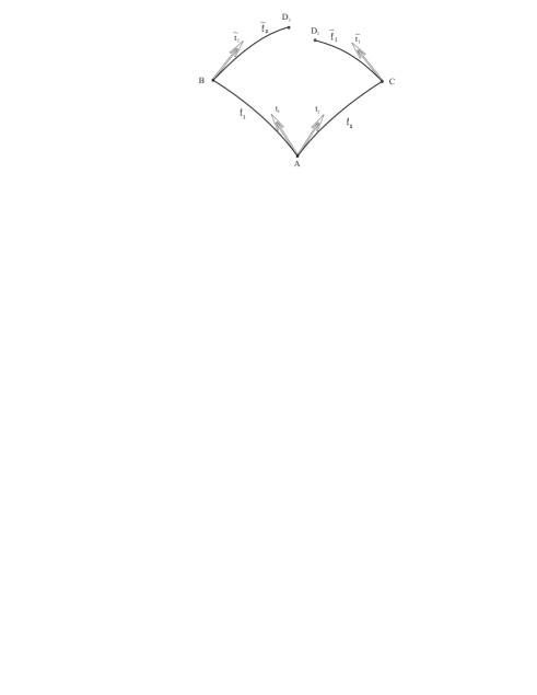
Figure 1: Geometrical meaning of the torsion.

In the curved space-time, this figure is not necessary closed. The difference of the coordinates at the points $D_{2}$ and $D_{1}$ is proportional to the torsion

$$x^{\mu}(D_{2})-x^{\mu}(D_{1})={}^{\circ}T^{\mu}{}_{\rho\sigma}\,t_{1}^{\rho}\,t_{2}^{\sigma}\,d\ell_{1}\,d\ell_{2}\,.$$ (6)

In fact the torsion measures the non-closure of the ”rectangle” $ABCD$.

The metric tensor $G_{\mu\nu}$ is a new variable, independent on the connection. This is a non-degenerate symmetric tensor, which enables us to calculate scalar product $VU=G_{\mu\nu}V^{\mu}U^{\nu}$, in order to measure lengths and angles.

We already learned, that covariant derivative is responsible for the comparison of the vectors from different points. What variable is responsible for comparison of the lengths of the vectors? The square of the length of the vector $V^{\mu}(x)$ is $V^{2}(x)=G_{\mu\nu}(x)V^{\mu}(x)V^{\nu}(x)$. The square of the length of its parallel transport to the point $x+dx$, is ${}^{\circ}V_{\parallel}^{2}(x+dx)=G_{\mu\nu}(x+dx){}^{\circ}V^{\mu}_{\parallel}\,{}^{\circ}V^{\nu}_{\parallel}$. Let us stress, that we used the local metric tensors in both expressions and realized the parallel transport with the connection ${}^{\circ}\Gamma^{\rho}_{\nu\mu}$. If we remember the invariance of the scalar product under the parallel transport, than the difference of the squares of the vectors is

$${}^{\circ}\delta V^{2}={}^{\circ}V_{\parallel}^{2}(x+dx)-V^{2}(x)=[G_{\mu\nu}(x+dx)-G_{\mu\nu}(x)-{}^{\circ}\delta G_{\mu\nu}(x)]\,{}^{\circ}V^{\mu}_{\parallel}\,\,{}^{\circ}V^{\nu}_{\parallel}\,.$$ (7)

Up to the higher terms we have

$${}^{\circ}\delta V^{2}=[dG_{\mu\nu}(x)-{}^{\circ}\delta G_{\mu\nu}(x)]V^{\mu}V^{\nu}={}^{\circ}DG_{\mu\nu}V^{\mu}V^{\nu}\equiv-dx^{\rho}\,{}^{\circ}\!Q_{\rho\mu\nu}V^{\mu}V^{\nu}\,,$$ (8)

where we introduced the nonmetricity as a covariant derivative of the metric tensor

$${}^{\circ}Q_{\mu\rho\sigma}=-{}^{\circ}D_{\mu}G_{\rho\sigma}\,.$$ (9)

Beside the lengths, the nonmetricity also changes the angle between the vectors $V_{1}^{\mu}$ and $V_{2}^{\mu}$, according to the relation

$${}^{\circ}\delta\cos(\angle(V_{1},V_{2}))={1\over 2\sqrt{V_{1}^{2}V_{2}^{2}}}\left[2V_{1}^{\rho}V_{2}^{\sigma}-\left({V_{1}^{\rho}V_{1}^{\sigma}\over V_{1}^{2}}+{V_{2}^{\rho}V_{2}^{\sigma}\over V_{2}^{2}}\right)(V_{1}V_{2})\right]{}^{\circ}Q_{\mu\rho\sigma}dx^{\mu}\,.$$ (10)

Note that we performed the parallel transport of the vectors, but not of the metric tensor. It means that for length calculation in the point $x+dx$, we used the metric tensor $G_{\mu\nu}(x+dx)$, which lives in the same point, and not the tensor $G_{\mu\nu}+{}^{\circ}\delta G_{\mu\nu}$ obtained after parallel transport from the point $x$. The requirement for the equality of these two tensors is known in the literature as a metric postulate. In fact, it is just some kind of compatibility between the metric and connection, such that metric after parallel transport is equal to the local metric. Here we will not accept this requirement, because the difference of these two tensors is the origin of the nonmetricity. So, the nonmetricity measures the deformation of lengths and angles during the parallel transport.

We also define the Weyl vector as

$${}^{\circ}Q_{\mu}={1\over D}G^{\rho\sigma}{}^{\circ}Q_{\mu\rho\sigma}\,,$$ (11)

where $D$ is the number of space-time dimensions. When the traceless part of the nonmetricity vanishes

$${}^{\circ}Q\kern-12.0pt\nearrow_{\mu\rho\sigma}\equiv{}^{\circ}Q_{\mu\rho\sigma}-G_{\rho\sigma}{}^{\circ}Q_{\mu}=0\,,$$ (12)

the parallel transport preserves the angles but not the lengths. Such geometry is known as a Weyl geometry.

Following the paper [9], we can decomposed the given connection ${}^{\circ}\Gamma^{\mu}_{\nu\rho}$ in terms of the Christoffel connection, contortion and nonmetricity. If we introduce the Schouten braces according to the relation

$$\{\mu\rho\sigma\}=\sigma\mu\rho+\rho\sigma\mu-\mu\rho\sigma\,,$$ (13)

then the Christoffel connection (191), can be expressed as $\Gamma_{\mu,\rho\sigma}=\frac{1}{2}\partial_{\{\mu}G_{\rho\sigma\}}$. The contortion ${}^{\circ}K_{\mu\rho\sigma}$ is defined in terms of the torsion

$${}^{\circ}K_{\mu\rho\sigma}=\frac{1}{2}{}^{\circ}T_{\{\sigma\mu\rho\}}=\frac{1}{2}({}^{\circ}T_{\rho\sigma\mu}+{}^{\circ}T_{\mu\rho\sigma}-{}^{\circ}T_{\sigma\mu\rho})\,.$$ (14)

By definition, the contortion is antisymmetric under first two indices ${}^{\circ}K_{\mu\rho\sigma}=-{}^{\circ}K_{\rho\mu\sigma}$.

The Schouten braces of the nonmetricity can be solved in terms of the connection

$${}^{\circ}\Gamma_{\mu,\rho\sigma}=\Gamma_{\mu,\rho\sigma}+{}^{\circ}K_{\mu\rho\sigma}+\frac{1}{2}{}^{\circ}Q_{\{\mu\rho\sigma\}}\,.$$ (15)

The first term is the Christoffel connection , which depends on the metric but which does not transforms as a tensor. The second one is the contortion (14) and the third one is Schouten braces of the nonmetricity (9). The last two terms transform as a tensors.

The first and third terms are symmetric in $\rho,\sigma$ indices. In the second term we can separate symmetric and antisymmetric parts, ${}^{\circ}K_{\mu\rho\sigma}={}^{\circ}K_{\mu(\rho\sigma)}+\frac{1}{2}{}^{\circ}T_{\mu\rho\sigma}$, where he symmetric part of the arbitrary tensor $X_{\mu\nu}$ we denote as $X_{(\mu\nu)}\equiv\hbox{${1\over 2}$}(X_{\mu\nu}+X_{\nu\mu})$. Consequently, we have

$${}^{\circ}\Gamma^{\mu}_{\rho\sigma}={}^{\circ}\Gamma^{\mu}_{(\rho\sigma)}+\frac{1}{2}{}^{\circ}T^{\mu}_{\rho\sigma}\,.$$ (16)

2.2 Induced and extrinsic geometry

Let $x^{\mu}(\xi)\,(\mu=0,1,...,D-1)$ be the coordinates of the $D$ dimensional space-time $M_{D}$ and $\xi^{\alpha}\,(\xi^{0}=\tau,\xi^{1}=\sigma)$ the coordinates of two dimensional world-sheet $\Sigma$, spanned by the string. The corresponding derivatives we will denote as $\partial_{\mu}\equiv{\partial\over\partial x^{\mu}}$ and $\partial_{\alpha}\equiv{\partial\over\partial\xi^{\alpha}}$. We will use the local space-time basis, relating with the coordinate one by the vielbein $E^{\mu}_{A}=\{\partial_{\alpha}x^{\mu},n_{i}^{\mu}\}$. Here, $\partial_{\alpha}x^{\mu}=\{{\dot{x}^{\mu}},x^{\prime\mu}\}$ is local world-sheet basis and $n^{\mu}_{i}\,(i=2,3,...,D-1)$ are local unit vectors, normal to the world-sheet.

The two dimensional induced metric tensor is defined by the requirement, that any world-sheet interval measured by the target space metric, has the same length as measured by the induced one. For a given space-time metric tensor $G_{\mu\nu}$, the world-sheet induced metric tensor takes the form

$$G_{\alpha\beta}=G_{\mu\nu}\partial_{\alpha}x^{\mu}\partial_{\beta}x^{\nu}\,.$$ (17)

Similarly, the induced metric of a $D-2$ dimensional space, normal to the world-sheet, is $G_{ij}=G_{\mu\nu}n_{i}^{\mu}n_{j}^{\nu}$. The mixed induced metric tensor $G_{\alpha i}=G_{\mu\nu}\partial_{\alpha}x^{\mu}n_{i}^{\nu}$, vanishes by definition.

The world-sheet projection and the orthogonal projection of the arbitrary space-time covector $V_{\mu}$, we will denote as

$$v_{\alpha}=\partial_{\alpha}x^{\mu}V_{\mu}\,,\qquad v_{i}=n_{i}^{\mu}V_{\mu}\,.$$ (18)

In the space-time basis, tangent and normal vectors to the world-sheet $\Sigma$ can be expressed respectively as

$$V^{\mu}_{\Sigma}=\partial_{\alpha}x^{\mu}v^{\alpha}\,,\qquad V^{\mu}_{\perp}=n_{i}^{\mu}v^{i}\,.$$ (19)

a) Parallel transport of the world-sheet tangent covectors. Let us perform the parallel transport of the covector $V_{\mu}^{\Sigma}$ along world-sheet line, from the point $\xi^{\alpha}$ to the point $\xi^{\alpha}+d\xi^{\alpha}$, using the space-time connection ${}^{\circ}\Gamma^{\nu}_{\mu\rho}$ (Fig. 2). We obtain the covector

$${}^{\circ}V^{\Sigma}_{\parallel\mu}=V^{\Sigma}_{\mu}+{}^{\circ}\delta V^{\Sigma}_{\mu}\,,$$ (20)

where

$${}^{\circ}\delta V_{\mu}^{\Sigma}={}^{\circ}\Gamma^{\nu}_{\mu\rho}V_{\nu}^{\Sigma}dx^{\rho}={}^{\circ}\Gamma^{\nu}_{\mu\rho}V_{\nu}^{\Sigma}\partial_{\gamma}x^{\rho}d\xi^{\gamma}\,.$$ (21)

In the local basis, at the point $\xi+d\xi$, its world-sheet projection has the form

$${}^{\circ}v_{\parallel\alpha}^{\Sigma}=\partial_{\alpha}x^{\mu}(\xi+d\xi){}^{\circ}V^{\Sigma}_{\parallel\mu}\,.$$ (22)

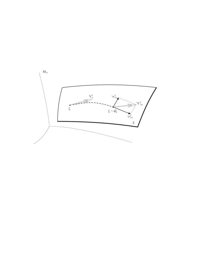
Figure 2: Definition of the induced connection ${}^{\circ}\Gamma^{\beta}_{\alpha\gamma}$ and SFF ${}^{\circ}{\bar{b}}_{i\alpha\beta}$ from the parallel transport of the world-sheet tangent covector. Here ${}^{\circ}v_{\parallel\alpha}^{\Sigma}\equiv v_{\alpha}+{}^{\circ}\Gamma^{\beta}_{\alpha\gamma}v_{\beta}\,d\xi^{\gamma}\,$ and ${}^{\circ}v^{\Sigma}_{\parallel i}\equiv-{}^{\circ}{\bar{b}}_{i\alpha\beta}\,v^{\alpha}d\xi^{\beta}$.

Let us introduce the world-sheet induced connection ${}^{\circ}\Gamma^{\beta}_{\alpha\gamma}$. We demand that it defines the rule of the parallel transport of the world-sheet covector $v_{\alpha}$, along the same world-sheet line, to the projection ${}^{\circ}v_{\parallel\alpha}^{\Sigma}$. So, we have by definition

$${}^{\circ}v_{\parallel\alpha}^{\Sigma}=v_{\alpha}+{}^{\circ}\delta v_{\alpha}\,,$$ (23)

where

$${}^{\circ}\delta v_{\alpha}={}^{\circ}\Gamma^{\beta}_{\alpha\gamma}v_{\beta}d\xi^{\gamma}\,.$$ (24)

It produce the expression for the induced connection

$${}^{\circ}\Gamma^{\gamma}_{\alpha\beta}=G^{\gamma\delta}\partial_{\delta}x^{\mu}G_{\mu\nu}({}^{\circ}\Gamma_{\rho\sigma}^{\nu}\partial_{\alpha}x^{\rho}\partial_{\beta}x^{\sigma}+\partial_{\beta}\partial_{\alpha}x^{\nu})=G^{\gamma\delta}\partial_{\delta}x^{\mu}G_{\mu\nu}{}^{\circ}D_{\beta}\partial_{\alpha}x^{\nu}\,,$$ (25)

where ${}^{\circ}D_{\alpha}V^{\mu}=\partial_{\alpha}x^{\nu}{}^{\circ}D_{\nu}V^{\mu}$ is space-time covariant derivative along world-sheet direction.

The orthogonal projection of the covector ${}^{\circ}V^{\Sigma}_{\parallel\mu}\,$, defines the second fundamental form, ${}^{\circ}{\bar{b}}_{i\alpha\beta}\,$, trough the equation

$$n_{i}^{\mu}(\xi+d\xi){}^{\circ}V^{\Sigma}_{\parallel\mu}\equiv{}^{\circ}v^{\Sigma}_{\parallel i}=-{}^{\circ}{\bar{b}}_{i\alpha\beta}v^{\alpha}d\xi^{\beta}\,,$$ (26)

or explicitly

$${}^{\circ}{\bar{b}}_{i\alpha\beta}=n_{i}^{\mu}\,{}^{\circ}\!D_{\beta}(G_{\mu\nu}\partial_{\alpha}x^{\nu})=-\partial_{\alpha}x^{\nu}G_{\mu\nu}{}^{\circ}\!D_{\beta}n_{i}^{\mu}\,.$$ (27)

The SFF define the extrinsic geometry.

b) Parallel transport of the world-sheet orthogonal covectors. If we perform parallel transport of the covector $V_{\mu}^{\bot}$, orthogonal to the world-sheet (Fig. 3), we obtain

$${}^{\circ}V^{\bot}_{\parallel\mu}=V^{\bot}_{\mu}+{}^{\circ}\delta V^{\bot}_{\mu}\,,\qquad{}^{\circ}\delta V^{\bot}_{\mu}={}^{\circ}\Gamma^{\nu}_{\mu\rho}V^{\bot}_{\nu}dx^{\rho}={}^{\circ}\Gamma^{\nu}_{\mu\rho}V^{\bot}_{\nu}\partial_{\alpha}x^{\rho}d\xi^{\alpha}\,.$$ (28)

Its normal projection, defines the induced connection of the $D-2$ dimensional space, normal to the world-sheet

$${}^{\circ}\Gamma^{i}_{j\alpha}=G^{ik}n^{\mu}_{k}G_{\mu\nu}{}^{\circ}D_{\alpha}n^{\nu}_{j}\,,$$ (29)

and its world-sheet projection defines also the SFF, which we denote by ${}^{\circ}b_{i\alpha\beta}$

$$\partial_{\alpha}x^{\mu}(\xi+d\xi){}^{\circ}V^{\bot}_{\parallel\mu}\equiv{}^{\circ}v^{\bot}_{\parallel\alpha}=v^{i}\,{}^{\circ}b_{i\alpha\beta}d\xi^{\beta}\,.$$ (30)

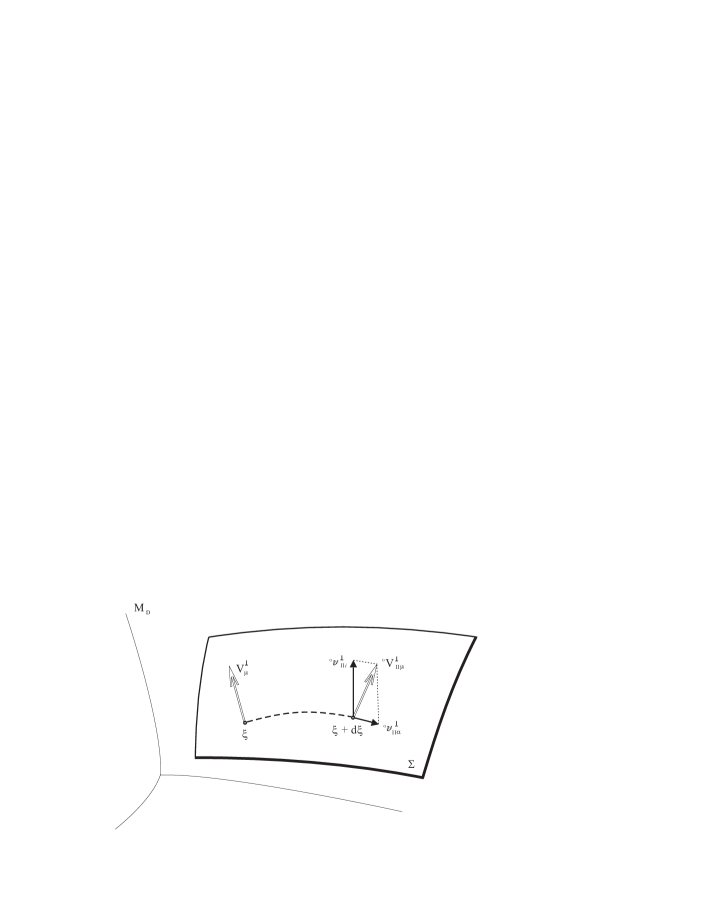
Figure 3: Definition of the induced connection ${}^{\circ}\Gamma^{j}_{i\alpha}$ and SFF ${}^{\circ}b_{i\alpha\beta}$ from the parallel transport of the world-sheet orthogonal covector. Here ${}^{\circ}v^{\bot}_{\parallel\alpha}\equiv{}^{\circ}b_{i\alpha\beta}\,v^{i}d\xi^{\beta}\,$ and ${}^{\circ}v_{\parallel i}^{\bot}\equiv v_{i}+{}^{\circ}\Gamma^{j}_{i\alpha}v_{j}\,d\xi^{\alpha}\,$.

Note that the expression for this new SFF

$${}^{\circ}b_{i\alpha\beta}=n_{i}^{\mu}G_{\mu\nu}{}^{\circ}D_{\beta}\partial_{\alpha}x^{\nu}=-\partial_{\alpha}x^{\nu}{}^{\circ}D_{\beta}(G_{\mu\nu}n_{i}^{\mu})\,,$$ (31)

differs from the previous one (27) by the term containing the covariant derivative of the metric. So, in the spaces with nonmetricity, there are two forms of SFF, connected by the relation

$${}^{\circ}b_{i\alpha\beta}={}^{\circ}{\bar{b}}_{i\alpha\beta}+{}^{\circ}Q_{\rho\mu\nu}\partial_{\beta}x^{\rho}n^{\mu}_{i}\partial_{\alpha}x^{\nu}\,.$$ (32)

c) Parallel transport of the world-sheet vectors. In the similar procedure for the vectors $V^{\mu}_{\Sigma}$ and $V^{\mu}_{\bot}$, the orthogonal projection of the ${}^{\circ}V^{\mu}_{\Sigma\parallel}$ produce $\,-{}^{\circ}b_{i\alpha\beta}$ and the world-sheet projection of ${}^{\circ}V^{\mu}_{\bot\parallel}$ produce ${}^{\circ}{\bar{b}}_{i\alpha\beta}$.

In analogy with the previous result, we define the bar induced connection through the relation

$$v_{\alpha}+{}^{\circ}{\bar{\delta}}v_{\alpha}=\partial_{\alpha}x^{\mu}(\xi+d\xi)G_{\mu\nu}(\xi+d\xi){}^{\circ}V^{\nu}_{\Sigma\parallel}\,,$$ (33)

where

$${}^{\circ}{\bar{\delta}}v_{\alpha}={}^{\circ}{\bar{\Gamma}}^{\beta}_{\alpha\gamma}v_{\beta}d\xi^{\gamma}\,.$$ (34)

Then, we have

$${}^{\circ}{\bar{\Gamma}}_{\gamma,\alpha\beta}=\partial_{\gamma}x^{\nu}{}^{\circ}D_{\beta}(G_{\mu\nu}\partial_{\alpha}x^{\mu})={}^{\circ}\Gamma_{\gamma,\alpha\beta}-{}^{\circ}Q_{\rho\mu\nu}\partial_{\beta}x^{\rho}\partial_{\alpha}x^{\mu}\partial_{\gamma}x^{\nu}\,,$$ (35)

which relates the two forms of the induced connections up to the nonmetricity term.

So, the induced connection and the SFF are projections, of the space-time covariant derivative of $\partial_{\alpha}x^{\mu}$, to the world-sheet and its normal, respectively. Consequently, we have the generalization of the Gauss-Weingarten equation

$${}^{\circ}\!D_{\beta}\partial_{\alpha}x^{\mu}={}^{\circ}\Gamma^{\gamma}_{\alpha\beta}\partial_{\gamma}x^{\mu}+{}^{\circ}b^{i}_{\alpha\beta}\,n_{i}^{\mu}\,,$$ (36)

and

$${}^{\circ}\!D_{\beta}(G_{\mu\nu}\partial_{\alpha}x^{\nu})=({}^{\circ}{\bar{\Gamma}}^{\gamma}_{\alpha\beta}\partial_{\gamma}x^{\nu}+{}^{\circ}{\bar{b}}^{i}_{\alpha\beta}\,n_{i}^{\nu})G_{\mu\nu}\,.$$ (37)

There are also two forms of the world-sheet induced covariant derivatives, corresponding to two forms of the world-sheet connections

$${}^{\circ}\nabla_{\alpha}v_{\beta}=\partial_{\alpha}v_{\beta}-{}^{\circ}\Gamma^{\gamma}_{\beta\alpha}v_{\gamma}\,,\qquad{}^{\circ}{\bar{\nabla}}_{\alpha}v_{\beta}=\partial_{\alpha}v_{\beta}-{}^{\circ}{\bar{\Gamma}}^{\gamma}_{\beta\alpha}v_{\gamma}\,.$$ (38)

They are related by the expression

$${}^{\circ}{\bar{\nabla}}_{\alpha}v_{\beta}={}^{\circ}\nabla_{\alpha}v_{\beta}+{}^{\circ}Q_{\alpha\beta\gamma}v^{\gamma}=G_{\beta\gamma}{}^{\circ}\nabla_{\alpha}v^{\gamma}\,.$$ (39)

From this point we will use the variables without bar, because the bar variables can be expressed in terms of the first ones and nonmetricity.

2.3 Decomposition of the induced connection ${}^{\circ}\Gamma^{\gamma}_{\alpha\beta}$ and of the SFF ${}^{\circ}b_{i\alpha\beta}$

In analogy with the general rule for connection decomposition, we can decompose the induced connection and SFF. With the help of (15) we have

$${}^{\circ}D_{\beta}\partial_{\alpha}x^{\mu}=D_{\beta}\partial_{\alpha}x^{\mu}+\left({}^{\circ}K^{\mu}{}_{\nu\rho}+\hbox{${1\over 2}$}{}^{\circ}Q^{\{\mu}{}_{\nu\rho\}}\right)\partial_{\alpha}x^{\nu}\partial_{\beta}x^{\rho}\,.$$ (40)

The world-sheet projection of the last equation, produces the decomposition of the induced connection

$${}^{\circ}\Gamma_{\gamma,\alpha\beta}=\Gamma_{\gamma,\alpha\beta}+{}^{\circ}K_{\gamma\alpha\beta}+\frac{1}{2}{}^{\circ}Q_{\{\gamma\alpha\beta\}}\,,$$ (41)

in terms of induced Christoffel connection, induced torsion and induced nonmetricity

$$\Gamma^{\gamma}_{\alpha\beta}=G^{\gamma\delta}\partial_{\delta}x^{\mu}\,G_{\mu\nu}{}^{\circ}\!D_{\beta}\partial_{\alpha}x^{\nu}\,,$$ (42)

$${}^{\circ}T_{\alpha\beta\gamma}={}^{\circ}T_{\mu\rho\sigma}\partial_{\alpha}x^{\mu}\partial_{\beta}x^{\rho}\partial_{\gamma}x^{\sigma}={}^{\circ}\Gamma_{\alpha,\beta\gamma}-{}^{\circ}\Gamma_{\alpha,\gamma\beta}\,,$$ (43)

$${}^{\circ}Q_{\alpha\beta\gamma}={}^{\circ}Q_{\mu\rho\sigma}\partial_{\alpha}x^{\mu}\partial_{\beta}x^{\rho}\partial_{\gamma}x^{\sigma}=-{}^{\circ}\nabla_{\alpha}G_{\beta\gamma}\,,$$ (44)

where ${}^{\circ}K_{\gamma\alpha\beta}=\hbox{${1\over 2}$}{}^{\circ}T_{\{\gamma\alpha\beta\}}$ is the induced contortion. Note that both the torsion and nonmetricity are tensors, so that the corresponding relations do not have non-homogeneous terms.

The orthogonal projection of (40) produces the decomposition of the SFF

$${}^{\circ}b_{i\alpha\beta}=b_{i\alpha\beta}+{}^{\circ}\!K_{i\alpha\beta}+\hbox{${1\over 2}$}{}^{\circ}\!Q_{\{i\alpha\beta\}}\equiv b_{i\alpha\beta}+{}^{\circ}\!\stackrel{{\scriptstyle K}}{{b}}_{i\alpha\beta}+\hbox{${1\over 2}$}{}^{\circ}\!\stackrel{{\scriptstyle Q}}{{b}}_{\{i\alpha\beta\}}\,,$$ (45)

where we used the notation

$$b_{i\alpha\beta}=n_{i}^{\mu}G_{\mu\nu}D_{\beta}\partial_{\alpha}x^{\nu}\,,$$ (46)

$${}^{\circ}\!\stackrel{{\scriptstyle T}}{{b}}_{i\alpha\beta}={}^{\circ}T_{\mu\rho\sigma}n_{i}^{\mu}\partial_{\alpha}x^{\rho}\partial_{\beta}x^{\sigma}\equiv{}^{\circ}T_{i\alpha\beta}\,,$$ (47)

$${}^{\circ}\!\stackrel{{\scriptstyle Q}}{{b}}_{i\alpha\beta}={}^{\circ}\!Q_{\mu\rho\sigma}n_{i}^{\mu}\partial_{\alpha}x^{\rho}\partial_{\beta}x^{\sigma}\equiv{}^{\circ}\!Q_{i\alpha\beta}\,,$$ (48)

and similarly as before ${}^{\circ}K_{i\alpha\beta}=\hbox{${1\over 2}$}{}^{\circ}T_{\{i\alpha\beta\}}$.

Consequently, with the help of (36) we have

$$D_{\beta}\partial_{\alpha}x^{\mu}=\Gamma^{\gamma}_{\alpha\beta}\,\partial_{\gamma}x^{\mu}+b^{i}_{\alpha\beta}\,n_{i}^{\mu}\,,$$ (49)

$${}^{\circ}T^{\mu}{}_{\rho\sigma}\partial_{\alpha}x^{\rho}\partial_{\beta}x^{\sigma}\equiv{}^{\circ}T^{\mu}{}_{\alpha\beta}={}^{\circ}T^{\gamma}{}_{\alpha\beta}\partial_{\gamma}x^{\mu}+{}^{\circ}\!T^{i}_{\alpha\beta}\,n_{i}^{\mu}\,,$$ (50)

$${}^{\circ}\!Q^{\mu}{}_{\rho\sigma}\partial_{\alpha}x^{\rho}\partial_{\beta}x^{\sigma}\equiv{}^{\circ}\!Q^{\mu}{}_{\alpha\beta}={}^{\circ}Q^{\gamma}{}_{\alpha\beta}\partial_{\gamma}x^{\mu}+{}^{\circ}\!Q^{i}_{\alpha\beta}\,n_{i}^{\mu}\,.$$ (51)

When the torsion is present, the SFF is not symmetric in $\alpha,\beta$ indices. Similarly as in the case of the connection, we can write

$${}^{\circ}b_{i\alpha\beta}={}^{\circ}b_{i(\alpha\beta)}+\hbox{${1\over 2}$}{}^{\circ}T_{i\alpha\beta}\,,\qquad{}^{\circ}b_{i(\alpha\beta)}=b_{i\alpha\beta}+{}^{\circ}K_{i(\alpha\beta)}+\hbox{${1\over 2}$}{}^{\circ}Q_{\{i\alpha\beta\}}\,.$$ (52)

2.4 Relations between space-time and world-sheet covariant derivatives

Starting with the definition of the space-time covariant derivatives along world-sheet direction

$${}^{\circ}DV^{\mu}=V^{\mu}(\xi+d\xi)-V^{\mu}_{\parallel}\,,$$ (53)

we can obtain its world-sheet and orthogonal projections, multiplying (53) with $G_{\mu\nu}(\xi+d\xi)\partial_{\alpha}x^{\nu}(\xi+d\xi)$ and $G_{\mu\nu}(\xi+d\xi)n^{\nu}_{i}(\xi+d\xi)$, respectively

$$\partial_{\alpha}x^{\nu}G_{\mu\nu}{}^{\circ}\!D_{\beta}V^{\mu}={}^{\circ}{\bar{\nabla}}_{\beta}v_{\alpha}-v^{i}\,{}^{\circ}\!{\bar{b}}_{i\alpha\beta}\,,\qquad n_{i}^{\nu}G_{\mu\nu}{}^{\circ}D_{\alpha}V^{\mu}={}^{\circ}{\bar{\nabla}}_{\alpha}v_{i}+v^{\beta}\,{}^{\circ}b_{i\beta\alpha}\,.$$ (54)

With the help of the relation $V^{\mu}=\partial_{\alpha}x^{\mu}v^{\alpha}+n_{i}^{\mu}v^{i}$ we obtain

$${}^{\circ}D_{\alpha}V^{\mu}={}^{\circ}\nabla_{\alpha}v^{\beta}\,\partial_{\beta}x^{\mu}+n_{i}^{\mu}\,{}^{\circ}b^{i}_{\beta\alpha}v^{\beta}+n_{i}^{\mu}G^{ij}\,{}^{\circ}{\bar{\nabla}}_{\alpha}v_{j}-\partial_{\beta}x^{\mu}v^{i}G^{\beta\gamma}\,{}^{\circ}\!{\bar{b}}_{i\gamma\alpha}\,.$$ (55)

Similarly, for the covectors we have

$${}^{\circ}D_{\alpha}V_{\mu}=G_{\mu\nu}\left[G^{\beta\gamma}\partial_{\beta}x^{\nu}{}^{\circ}\nabla_{\alpha}v_{\gamma}+n_{i}^{\nu}\,{}^{\circ}{\bar{b}}^{i}_{\beta\alpha}v^{\beta}\right]+G_{\mu\nu}\left[G^{ij}n_{i}^{\nu}{}^{\circ}\nabla_{\alpha}v_{j}-G^{\beta\gamma}\partial_{\beta}x^{\nu}v^{i}\,{}^{\circ}b_{i\gamma\alpha}\right]\,.$$ (56)

For the world-sheet tangent vectors, the last two equations produce

$${}^{\circ}D_{\alpha}V^{\mu}_{\Sigma}={}^{\circ}\nabla_{\alpha}v^{\beta}\,\partial_{\beta}x^{\mu}+n_{i}^{\mu}\,{}^{\circ}b^{i}_{\beta\alpha}v^{\beta}\,,$$ (57)

$${}^{\circ}D_{\alpha}V_{\mu}^{\Sigma}=G_{\mu\nu}\left[G^{\beta\gamma}\partial_{\beta}x^{\nu}\,{}^{\circ}\nabla_{\alpha}v_{\gamma}+n_{i}^{\nu}\,{}^{\circ}{\bar{b}}^{i}_{\beta\alpha}v^{\beta}\right]\,.$$ (58)

We will also need the relation

$$({}^{\circ}D_{\alpha}V_{\mu})\partial_{\beta}x^{\mu}={}^{\circ}\nabla_{\alpha}v_{\beta}-v^{i}\,{}^{\circ}b_{i\beta\alpha}\,,$$ (59)

obtaining multiplying (56) by $\partial_{\beta}x^{\mu}$.

2.5 Mean extrinsic curvature

In the torsion free case, the SFF is symmetric in the world-sheet indices and its properties are well known in the literature. Here, we will consider the case when nontrivial torsion and nonmetricity are present.

As usual, a curve is parametrized by its length parameter $s$, so that the unit tangent vector is $t^{\mu}={dx^{\mu}\over ds}$. If the curve lies in the world-sheet, we have $t^{\mu}=t^{\alpha}\partial_{\alpha}x^{\mu}$, with $t^{\alpha}={d\xi^{\alpha}\over ds}$. Let us denote by $P_{i}$, the 2-plane spanned by the tangent vector $t^{\mu}$ and the unit world-sheet normal $n_{i}^{\mu}$. Then, $\ell_{i}=\Sigma\bigcap P_{i}$ is the $i$-th normal section of the world-sheet $\Sigma$. The curvature of the normal section $\ell_{i}$, as a space-time curve, is defined as the orthogonal projection of ${}^{\circ}D_{s}t^{\mu}$

$${}^{\circ}k_{i}={}^{\circ}D_{s}t^{\mu}G_{\mu\nu}n^{\nu}_{i}\,,$$ (60)

where ${}^{\circ}D_{s}t^{\mu}\equiv{\dot{x}}^{\nu}{}^{\circ}D_{\nu}t^{\mu}$, is the covariant derivative along the curve. It produces the following expression

$${}^{\circ}k_{i}={}^{\circ}b_{i\beta\alpha}\,t^{\alpha}t^{\beta}={}^{\circ}b_{i(\beta\alpha)}\,t^{\alpha}t^{\beta}={{}^{\circ}b_{i(\beta\alpha)}d\xi^{\alpha}d\xi^{\beta}\over G_{\alpha\beta}d\xi^{\alpha}d\xi^{\beta}}\,.$$ (61)

The curvature ${}^{\circ}k_{i}$ depends on the direction of the tangent vector $t^{\alpha}$ and only on the symmetric part of the SFF. Let us stress, that in the presence of nonmetricity, ${}^{\circ}D_{s}t^{\mu}$ is not orthogonal to the tangent vector $t^{\mu}$, and we additionally performed orthogonal projection.

In Euclidean torsion free spaces, the maximal and minimal values of ${}^{\circ}\!k_{i}$ are the principal curvatures. The corresponding directions, defined by $t^{\alpha}$, are the principal directions. The principal curvatures are eigenvalues of the SFF and corresponding eigenvectors define the principal directions.

In our case, the curvature ${}^{\circ}\!k_{i}$, (61), is divergent in the light-cone directions. Consequently, the extremely values do not exist. Still, we can obtain the necessary information from the eigenvalue problem

$$({}^{\circ}\!b^{i}_{\alpha\beta}-{}^{\circ}\!\kappa^{i}G_{\alpha\beta})v^{\beta}=0\,.$$ (62)

The eigenvalues of the quadratic forms ${}^{\circ}b^{i}_{\alpha\beta}$ with respect to the metric $G_{\alpha\beta}$, we define as a principal curvatures in Minkowski space-time. They are the solutions of the condition $\det({}^{\circ}\!b^{i}-{}^{\circ}\!\kappa^{i}G)_{\alpha\beta}=0$, or explicitly

$${}^{\circ}\!\kappa^{i}_{0,1}={}^{\circ}\!H^{i}\pm\sqrt{({}^{\circ}\!H^{i})^{2}-{}^{\circ}\!K^{i}}\,.$$ (63)

Here

$${}^{\circ}\!H^{i}=\hbox{${1\over 2}$}G^{\alpha\beta}{}^{\circ}\!b^{i}_{\alpha\beta}\,=\hbox{${1\over 2}$}({}^{\circ}\!\kappa^{i}_{0}+{}^{\circ}\!\kappa^{i}_{1})\,,$$ (64)

is the trace of the SFF and ${}^{\circ}\!K^{i}={\det{}^{\circ}\!b^{i}_{\alpha\beta}\over\det G_{\alpha\beta}}={}^{\circ}\!\kappa^{i}_{0}{}^{\circ}\!\kappa^{i}_{1}$ (no summation over $i$) is Gauss curvature.

In order to simplify the relation (61), we will go to the new frame in which both symmetric matrices, $G_{\alpha\beta}$ and ${}^{\circ}b_{i(\alpha\beta)}$, are diagonal. We can choose the eigenvectors ($v_{0}^{\alpha}$, $v_{1}^{\alpha}$) of the symmetric part of the SFF ${}^{\circ}\!b^{i}_{(\alpha\beta)}$, as new basis vectors. Then, instead of (62) we have $({}^{\circ}\!b^{i}_{(\alpha\beta)}-{}^{\circ}\!\kappa^{i}G_{\alpha\beta})v^{\beta}=0$, which produces $({}^{\circ}\!\kappa^{i}_{0}-{}^{\circ}\!\kappa^{i}_{1})(v_{0}^{\alpha}G_{\alpha\beta}v_{1}^{\beta})=0$. For ${}^{\circ}\!\kappa^{i}_{0}\neq{}^{\circ}\!\kappa^{i}_{1}$, the eigenvectors are orthogonal. Let us chose $v_{0}$ to be time-like vector and $v_{1}$ to be space-like vector, and normalize them as $v_{0}^{2}=1,\,\,v_{1}^{2}=-1$. In the basis ($v_{0},v_{1}$), both the metric and the symmetric part of the SFF, obtain diagonal forms

$$G=\pmatrix{1&0\cr 0&-1\cr}\,,\qquad b_{i}=\pmatrix{{}^{\circ}\!\kappa^{i}_{0}&0\cr 0&-{}^{\circ}\!\kappa^{i}_{1}\cr}\,.$$ (65)

The curvature of the line $\ell_{i}$ becomes

$${}^{\circ}k^{i}_{tl}(\alpha)={}^{\circ}\!\kappa^{i}_{0}\cosh^{2}(\alpha)-{}^{\circ}\!\kappa^{i}_{1}\sinh^{2}(\alpha)\,,$$ (66)

where $\alpha\in(-\infty,\infty)$ parametrize all time-like directions of the tangent vectors. Similarly, for the space-like tangent vectors, we have

$${}^{\circ}k^{i}_{sl}(\alpha)={}^{\circ}\!\kappa^{i}_{0}\sinh^{2}(\alpha)-{}^{\circ}\!\kappa^{i}_{1}\cosh^{2}(\alpha)\,.$$ (67)

The $i$-th MEC usually is defined as a mean value of the $i$-th normal section, if we fixed the normal $n_{i}^{\mu}$ and rotate the tangent vector $t^{\mu}$. In Euclidean spaces, the $\sin$ and $\cos$ functions appear instead of $\sinh$ and $\cosh$, so that the mean value is well defined. In Minkowski spaces, the curvature (61) is divergent in the light-like directions. We introduce the cut-off $\Lambda$, and define regularized mean curvature for the time-like region

$${}^{\circ}H^{i}_{tl}(\Lambda)={1\over 2\Lambda}\int_{-\Lambda}^{\Lambda}{}^{\circ}k^{i}_{tl}(\alpha)d\alpha\,,$$ (68)

and similarly for the space-like one. Finally, the mean extrinsic curvature we define as a mean value of the time-like mean curvature with sign $+$, and space-like mean curvature with sign $-$, with the same cut-off $\Lambda$ going to the infinity. We obtain

$$\lim_{\Lambda\to\infty}\hbox{${1\over 2}$}[{}^{\circ}H^{i}_{tl}(\Lambda)-{}^{\circ}H^{i}_{sl}(\Lambda)]=\hbox{${1\over 2}$}({}^{\circ}\!\kappa^{i}_{0}+{}^{\circ}\!\kappa^{i}_{1})={}^{\circ}\!H^{i}\,,$$ (69)

which is just the expression (64), because the $\Lambda$ dependence disappears.

For ${}^{\circ}\!\kappa^{i}_{0}={}^{\circ}\!\kappa^{i}_{1}\equiv{}^{\circ}\!\kappa^{i}$, all linear combinations of the vectors $v_{0}$ and $v_{1}$ are eigenvectors. We can choose some orthonormal basis, in which

$$G=\pmatrix{1&0\cr 0&-1\cr}\,,\qquad b_{i}=\pmatrix{{}^{\circ}\!\kappa^{i}&0\cr 0&-{}^{\circ}\!\kappa^{i}\cr}\,.$$ (70)

Then the line curvature does not depend on the tangent vector direction

$${}^{\circ}k^{i}_{tl}(\alpha) = {}^{\circ}\!\kappa^{i}[\cosh^{2}(\alpha)-\sinh^{2}(\alpha)]={}^{\circ}\!\kappa^{i}={}^{\circ}\!H^{i}_{tl}\,,$$

$${}^{\circ}k^{i}_{sl}(\alpha) = {}^{\circ}\!\kappa^{i}[\sinh^{2}(\alpha)-\cosh^{2}(\alpha)]=-{}^{\circ}\!\kappa^{i}={}^{\circ}\!H^{i}_{sl}\,.$$ (71)

Consequently, the MEC has the same interpretation $\hbox{${1\over 2}$}({}^{\circ}\!H^{i}_{tl}-{}^{\circ}\!H^{i}_{sl})={}^{\circ}\!\kappa^{i}={}^{\circ}\!H^{i}$.

The surface defined by the equation ${}^{\circ}\!H^{i}=0$ is minimal surface. The name stems from the fact that in the Riemann space-time the equation $H_{i}=0$ define the surface of minimal area $P_{2}=\int d^{2}\xi\sqrt{-\det G_{\alpha\beta}}\,$, for the fixed boundary. In fact, for this surface the first variation of the area vanishes

$$\delta P_{2}=-2\int d^{2}\xi\sqrt{-\det G_{\alpha\beta}}\,H^{i}n^{\mu}_{i}G_{\mu\nu}\,\delta x^{\nu}=0\,.$$ (72)

2.6 Dual mean extrinsic curvature, extrinsic mean torsion and C-duality

Let us stress that above consideration is torsion independent, because the antisymmetric part of the SFF disappears from (61) and (64). We are going to include the torsion contribution and generalize the above results.

Let us first generalize the eigenvalue problem, and then offer its geometrical interpretation. We introduce the dual eigenvalue problem, such that linear transformation of the vector $v^{\alpha}$ with operator ${}^{\circ}\!b^{i}_{\alpha\beta}$ is proportional to the two dimensional dual vector ${}^{\ast}v_{\alpha}=\sqrt{-G_{2}}\,\varepsilon_{\alpha\beta}\,v^{\beta}\,\,(G_{2}=\det G_{\alpha\beta})$

$${}^{\circ}\!b^{i}_{\alpha\beta}\,v^{\beta}={}^{\ast}\kappa^{i}\,{}^{\ast}v_{\alpha}\,,$$ (73)

or equivalently

$$\left({}^{\circ}\!b^{i}_{\alpha\beta}-{}^{\ast}\kappa^{i}\,\varepsilon_{\alpha\beta}\sqrt{-G_{2}}\right)v^{\beta}=0\,.$$ (74)

It is similar to (62), but for the completeness we also need the eigenvalues of the quadratic forms ${}^{\circ}b^{i}_{\alpha\beta}$ with respect to the antisymmetric tensor $\varepsilon_{\alpha\beta}\sqrt{-G_{2}}$.

The solutions of the condition $\det({}^{\ast}\!b^{i}-{}^{\ast}k^{i}\,\varepsilon\sqrt{-G_{2}})_{\alpha\beta}=0$, have the form

$${}^{\ast}\kappa^{i}_{0,1}={}^{\ast}H^{i}\pm\sqrt{({}^{\ast}H^{i})^{2}+{}^{\circ}\!K^{i}}\,.$$ (75)

In analogy with the previous case, we will call them dual principal curvatures, and the variable

$${}^{\ast}H^{i}=\hbox{${1\over 2}$}({}^{\ast}\kappa^{i}_{0}+{}^{\ast}\kappa^{i}_{1})=\hbox{${1\over 2}$}G^{\alpha\beta}{}^{\ast}b^{i}_{\alpha\beta}=\hbox{${1\over 2}$}{\varepsilon^{\alpha\beta}\over\sqrt{-G_{2}}}{}^{\circ}\!b^{i}_{\beta\alpha}=\hbox{${1\over 4}$}{\varepsilon^{\alpha\beta}\over\sqrt{-G_{2}}}{}^{\circ}\!T^{i}_{\beta\alpha}\,,$$ (76)

the dual mean extrinsic curvature. Here ${}^{\circ}\!K^{i}={\det{}^{\circ}\!b^{i}_{\alpha\beta}\over\det G_{\alpha\beta}}={}^{\ast}\kappa^{i}_{0}{}^{\ast}\kappa^{i}_{1}$ (no summation over $i$) is the same Gauss curvature as before.

Let us now turn to the geometrical meaning of the DMEC. In the case when $t^{\mu}_{1}$ and $t^{\mu}_{2}$ are world-sheet tangent vectors (Fif. 1) (note that all geodesics $\ell_{1}$, $\ell_{2}$, $\tilde{\ell}_{1}$ and $\tilde{\ell}_{2}$ still could be space-time curves) we can rewrite (6) in the form

$${}^{\circ}T^{\mu}\equiv{x^{\mu}(D_{2})-x^{\mu}(D_{1})\over 2dP_{12}}={\varepsilon^{\beta\alpha}\over 4\sqrt{-G_{2}}}\,{}^{\circ}T^{\mu}_{\rho\sigma}\partial_{\alpha}x^{\rho}\partial_{\beta}x^{\sigma}\,.$$ (77)

Here, $dP_{12}=\sqrt{-G_{2}}\det({\partial\xi^{\alpha}\over\partial s_{r}})d\ell_{1}d\ell_{2}$ is area of the parallelogram, spanned by the vectors $\ell_{1}^{\mu}=t_{1}^{\mu}d\ell_{1}$ and $\ell_{2}^{\mu}=t_{2}^{\mu}d\ell_{2}\,$, and where $G_{2}=\det G_{\alpha\beta}$. We can conclude that ${}^{\circ}T^{\mu}$ does not depend on the directions $t^{\mu}_{1}$ and $t^{\mu}_{2}$, and on the lengths $d\ell_{1}$ and $d\ell_{2}$. So, we will call this variable the mean torsion. Its world-sheet projection is induced mean torsion

$${}^{\circ}T_{\gamma}={}^{\circ}T^{\mu}G_{\mu\nu}\partial_{\gamma}x^{\nu}={\varepsilon^{\beta\alpha}\over 4\sqrt{-G_{2}}}\,{}^{\circ}T_{\gamma\alpha\beta}\,.$$ (78)

Its normal projection is the extrinsic mean torsion

$${}^{\circ}T_{i}={}^{\circ}T^{\mu}G_{\mu\nu}n_{i}^{\mu}={\varepsilon^{\beta\alpha}\over 4\sqrt{-G_{2}}}\,{}^{\circ}T_{i\alpha\beta}={}^{\ast}H_{i}\,,$$ (79)

which is exactly the same variable as DMEC, defined above in (76).

We can formulate the dual eigenvalue problem (74), as an ordinary eigenvalue problem $({}^{\ast}b^{i}_{\alpha\beta}-{}^{\ast}\kappa^{i}G_{\alpha\beta})v^{\alpha}=0$, if we introduce the dual SFF

$${}^{\ast}b^{i}_{\alpha\beta}={G_{\alpha\gamma}\varepsilon^{\gamma\delta}\over\sqrt{-G_{2}}}\,{}^{\circ}\!b^{i}_{\delta\beta}\,.$$ (80)

We define the C-duality (Curvature duality), which maps SFF to dual SFF, ${}^{\circ}b^{i}_{\alpha\beta}\to{}^{\ast}b^{i}_{\alpha\beta}$, and interchanges the role played by the symmetric and the antisymmetric parts of the SFF. Consequently, under C-duality MEC maps to DMEC, allowing the exchange of the mean curvature and mean torsion.

The self-dual and self-antidual configurations

$${}^{\circ}H^{i}=\pm{}^{\ast}H^{i}\,,$$ (81)

correspond to the following conditions on the SFF

$$(G^{\alpha\beta}\mp{\varepsilon^{\alpha\beta}\over\sqrt{-G_{2}}}){}^{\circ}\!b^{i}_{\beta\alpha}=0\,.$$ (82)

The equations (81) and (82) define C-dual (antidual) surfaces. In the torsion free case, they turn to the standard minimal surface condition, ${}^{\circ}H^{i}=0$.

3 The stringy geometry as a space-time perception by probe string

We are going to investigate the dynamics of the string, propagated in the curved space-time. From the mathematical point of view, the string equations of motion describe the embedding conditions of the world-sheet in the space-time. We are particularly interested in the target space geometry properties, recognized by the string. We will see, that the probe string feels more space-time features (torsion and nonmetricity) then the probe particle.

3.1 The action and the canonical analysis results

The action [2]-[5]

$$S=\kappa\int_{\Sigma}d^{2}\xi\sqrt{-g}\left\{\left[{1\over 2}g^{\alpha\beta}G_{\mu\nu}(x)+{\varepsilon^{\alpha\beta}\over\sqrt{-g}}B_{\mu\nu}(x)\right]\partial_{\alpha}x^{\mu}\partial_{\beta}x^{\nu}+\Phi(x)\stackrel{{\scriptstyle\omega}}{{R}}^{(2)}\right\}\,,$$ (83)

describes bosonic string propagation in $x^{\mu}$-dependent background fields: metric $G_{\mu\nu}$, antisymmetric tensor field $B_{\mu\nu}=-B_{\nu\mu}$ and dilaton field $\Phi$. Here, $g_{\alpha\beta}$ is the intrinsic world-sheet metric and $\stackrel{{\scriptstyle\omega}}{{R}}^{(2)}$ is corresponding scalar curvature. In App. A, we will introduce the intrinsic connection $\omega$, as a Christoffel connection for the intrinsic metric $g_{\alpha\beta}$. So, we mark all related variables with the sign $\omega$, in order to distinguish them from the corresponding induced ones.

In this paper we will restrict our consideration to such forms of the dilaton fields $\Phi$, that its gradient $a_{\mu}=\partial_{\mu}\Phi$, is not light-cone vector. So, the condition $a^{2}\equiv G^{\mu\nu}a_{\mu}a_{\nu}\neq 0$ is fulfilled in the whole space-time.

The projection operator

$$P^{T}{}_{\mu\nu}=G_{\mu\nu}-{a_{\mu}a_{\nu}\over a^{2}}=G_{\mu\nu}-\varepsilon n_{\mu}n_{\nu}\equiv G_{\mu\nu}^{D-1}\,,$$ (84)

($n_{\mu}={a_{\mu}\over\sqrt{\varepsilon a^{2}}}$, where $\varepsilon=1$ if $a_{\mu}$ is time like vector and $\varepsilon=-1$ if $a_{\mu}$ is space like vector), can be interpreted as the induced metric on the $D-1$ dimensional submanifold $\Phi(x)=const$.

Let us briefly review the result of the canonical analysis of ref. [1]. It is useful to define the currents

$$J_{\pm\mu}=P^{T}{}_{\mu}{}^{\nu}j_{\pm\nu}+{a_{\mu}\over 2a^{2}}i_{\pm}^{\Phi}=j_{\pm\mu}-{a_{\mu}\over a^{2}}j\,,$$ (85)

$$i_{\pm}^{F}={a^{\mu}\over a^{2}}j_{\pm\mu}-{1\over 2a^{2}}i_{\pm}^{\Phi}\pm 2\kappa{F^{\prime}}\,,\qquad i_{\pm}^{\Phi}=\pi_{F}\pm 2\kappa\Phi^{\prime}\,,$$ (86)

where

$$j_{\pm\mu}=\pi_{\mu}+2\kappa\Pi_{\pm\mu\nu}{x^{\nu}}^{\prime}\,,\qquad\Pi_{\pm\mu\nu}\equiv B_{\mu\nu}\pm{1\over 2}G_{\mu\nu}\,,$$ (87)

and

$$j=a^{\mu}j_{\pm\mu}-{1\over 2}i_{\pm}^{\Phi}=a^{2}(i_{\pm}^{F}\mp 2\kappa F^{\prime})\,.$$ (88)

All $\tau$ and $\sigma$ derivatives of the fields $x^{\mu}$, $F$ and $\Phi$ can be expressed in terms of the corresponding currents

$${\dot{x}}^{\mu}={G^{\mu\nu}\over 2\kappa}(h^{-}J_{-\nu}-h^{+}J_{+\nu})\,,$$ (89)

$${\dot{F}}={1\over 4\kappa}(h^{-}i_{-}^{F}-h^{+}i_{+}^{F})-{1\over 2}{(h^{-}+h^{+})^{\prime}}\,,\qquad{\dot{\Phi}}={1\over 4\kappa}(h^{-}i_{-}^{\Phi}-h^{+}i_{+}^{\Phi})\,,$$ (90)

and

$$x^{\mu\prime}={G^{\mu\nu}\over 2\kappa}(J_{+\nu}-J_{-\nu})\,,\qquad{F^{\prime}}={1\over 4\kappa}(i_{+}^{F}-i_{-}^{F})\,,\qquad{\Phi^{\prime}}={1\over 4\kappa}(i_{+}^{\Phi}-i_{-}^{\Phi})\,.$$ (91)

Up to boundary term, the canonical Hamiltonian density has the standard form

$${\cal H}_{c}=h^{-}T_{-}+h^{+}T_{+}\,.$$ (92)

The energy momentum tensor components obtain new expressions

$$T_{\pm}=\mp{1\over 4\kappa}\left(G^{\mu\nu}J_{\pm\mu}J_{\pm\nu}+i_{\pm}^{F}i_{\pm}^{\Phi}\right)+{1\over 2}i_{\pm}^{\Phi\prime}=\mp{1\over 4\kappa}\left(G^{\mu\nu}j_{\pm\mu}j_{\pm\nu}-{j^{2}\over a^{2}}\right)+i_{\pm}\,,$$ (93)

where

$$i_{\pm}={1\over 2}({i_{\pm}^{\Phi}}^{\prime}-F^{\prime}i_{\pm}^{\Phi})\,.$$ (94)

The same chirality energy-momentum tensor components satisfy two independent copies of Virasoro algebras,

$$\{T_{\pm},T_{\pm}\}=-[T_{\pm}(\sigma)+T_{\pm}({\bar{\sigma}})]{\delta^{\prime}}\,,$$ (95)

while the opposite chirality components commute $\{T_{\pm},T_{\mp}\}=0$. The energy-momentum tensor components $T_{\pm}$ are generators of the two dimensional diffeomorphisms. Their new, non-linear representation is the consequence of the dilaton field presence.

3.2 Equations of motion

In the paper [1], using canonical approach, we derived the following equations of motion

$$[J^{\mu}]\equiv\stackrel{{\scriptstyle\omega}}{{\nabla}}_{\mp}\partial_{\pm}x^{\mu}+{}^{\star}\Gamma_{\mp\rho\sigma}^{\mu}\partial_{\pm}x^{\rho}\partial_{\mp}x^{\sigma}=0\,,$$ (96)

$$[h^{\pm}]\equiv G_{\mu\nu}\partial_{\pm}x^{\mu}\partial_{\pm}x^{\nu}-2\stackrel{{\scriptstyle\omega}}{{\nabla}}_{\pm}\partial_{\pm}\Phi=0\,,$$ (97)

$$[i^{F}]\equiv\stackrel{{\scriptstyle\omega}}{{R}}^{(2)}+{2\over a^{2}}(D_{\mp\mu}a_{\nu})\partial_{\pm}x^{\nu}\partial_{\mp}x^{\mu}=0\,,$$ (98)

where the variables in the parenthesis denote the currents corresponding to this equation. The expression

$${}^{\star}\Gamma^{\rho}_{\pm\nu\mu}=\Gamma^{\rho}_{\pm\nu\mu}+{a^{\rho}\over a^{2}}D_{\pm\mu}a_{\nu}=P^{T\rho}{}_{\sigma}\Gamma^{\sigma}_{\pm\nu\mu}+{a^{\rho}\over a^{2}}\partial_{\mu}a_{\nu}=\Gamma^{\rho}_{\nu\mu}\pm P^{T\rho}{}_{\sigma}B^{\sigma}_{\nu\mu}+{a^{\rho}\over a^{2}}D_{\mu}a_{\nu}\,,\quad$$ (99)

which appears in the $[J^{\mu}]$ equation is a generalized connection, which full geometrical interpretation will be presented later. Under space-time general coordinate transformations the expression ${}^{\star}\Gamma^{\rho}_{\pm\nu\mu}$ transforms as a connection. In (96) and (98) we omit the currents $\pm$ indices, because $[J^{\mu}_{+}]=[J^{\mu}_{-}]$ and $[i^{F}_{+}]=[i^{F}_{-}]$ as a consequence of the symmetry relations ${}^{\star}\Gamma_{\mp\rho\sigma}^{\mu}={}^{\star}\Gamma_{\pm\sigma\rho}^{\mu}$ and $D_{\mp\mu}a_{\nu}=D_{\pm\nu}a_{\mu}$.

We can derive the Lagrangian equations of motion, independently of the previous consideration. Varying the action (83) with respect to $x^{\mu}$, we obtain

$$[x^{\mu}]\equiv g^{\alpha\beta}\stackrel{{\scriptstyle\omega}}{{\nabla}}_{\alpha}\partial_{\beta}x^{\mu}+\Gamma^{(\alpha\beta)\mu}{}_{\rho\sigma}\partial_{\alpha}x^{\rho}\partial_{\beta}x^{\sigma}-a^{\mu}\stackrel{{\scriptstyle\omega}}{{R}}^{(2)}=0\,,$$ (100)

where

$$\Gamma^{(\alpha\beta)\mu}{}_{\rho\sigma}=g^{\alpha\beta}\,\Gamma^{\mu}_{\rho\sigma}-{\varepsilon^{\alpha\beta}\over\sqrt{-g}}B^{\mu}_{\rho\sigma}\,.$$ (101)

Because in the light-cone basis we have $g^{\pm\pm}=0$ and $\varepsilon^{\pm\pm}=0$, the above expression has only two nonzero components

$$\Gamma^{(\mp\pm)\mu}{}_{\rho\sigma}=\Gamma^{\mu}_{\pm\rho\sigma}\,,\qquad\Gamma^{(\pm\pm)\mu}{}_{\rho\sigma}=0\,.$$ (102)

So, the expression ”two types of connections”, which has been used in the literature, means that in the light-cone basis there are just two nonzero elements of five indices expression (101). The connections $\Gamma^{\mu}_{\pm\rho\sigma}$ corresponds to the parallel transport along the light-cone lines $d\xi^{\pm}$, respectively. Trough the paper we will preserve the word connection, having in mind this comment.

Instead of the equations of motion with respect to the world-sheet metric $g_{\alpha\beta}$, we prefer to have ones with respect to the fields $F$ and $h^{\pm}$

$$[F]\equiv\stackrel{{\scriptstyle\omega}}{{\Delta}}\Phi=0\,,$$ (103)

$$T_{\pm}=\mp\frac{\kappa}{2}(G_{\mu\nu}{\partial}_{\pm}x^{\mu}{\partial}_{\pm}x^{\nu}-2\stackrel{{\scriptstyle\omega}}{{\nabla}}_{\pm}{\partial}_{\pm}\Phi-\stackrel{{\scriptstyle\omega}}{{\Delta}}\Phi)=0\,,$$ (104)

where the $T_{\pm}$ are energy-momentum tensor components in the light-cone basis.

Let us compare these equations with ones obtained before, using canonical methods. The equation (97) follows from (103) and (104). The equation (100) in the light-cone basic obtains the form

$$[x^{\mu}_{\pm}]\equiv\stackrel{{\scriptstyle\omega}}{{\nabla}}_{\mp}{\partial}_{\pm}x^{\mu}+\Gamma_{\mp\rho\sigma}^{\mu}{\partial}_{\pm}x^{\rho}{\partial}_{\mp}x^{\sigma}-\hbox{${1\over 2}$}a^{\mu}\stackrel{{\scriptstyle\omega}}{{R}}^{(2)}=0\,,$$ (105)

because $[x^{\mu}]=[x^{\mu}_{+}]+[x^{\mu}_{-}]$ and $[x^{\mu}_{+}]=[x^{\mu}_{-}]$ as a consequence of the above symmetry relations. Then we can conclude that $[i^{F}]$ and $[J^{\mu}]$ contain longitudinal and transversal parts of $[x^{\mu}]$ respectively

$$[i^{F}]=-{1\over a^{2}}\left(a_{\mu}[x^{\mu}]+[F]\right)\,,\qquad 2[J^{\mu}]=P^{T\mu}{}_{\nu}[x^{\nu}]+{a^{\mu}\over a^{2}}[F]\,.$$ (106)

We prefer the equations of motion in the form (96)-(98), with the canonical origin, because they are more appropriate for geometrical interpretation.

3.3 Stringy torsion and nonmetricity

Let us apply the general considerations of Sec. 2 to the string case. Instead of general mark ^∘, the mark ^⋆ will indicates the presence of nonmetricity felt by the string, and lower indices $\pm$ will indicate the presence of the corresponding form of torsion felt by the string. Absence of any sign will means that the connection is Christoffel.

The manifold $M_{D}$, together with the affine connection ${}^{\circ}\Gamma^{\mu}_{\nu\rho}$ and the metric $G_{\mu\nu}$, define the affine space-time $A_{D}\equiv(M_{D},{}^{\circ}\Gamma,G)$. The connection (99) we will call stringy connection and the corresponding space-time $S_{D}\equiv(M_{D},{}^{\star}\Gamma_{\pm},G)$, observed by the string propagating in the background $G_{\mu\nu}$, $B_{\mu\nu}$ and $\Phi$, we will call stringy space-time. The classification of space-times dependence on the background fields contributions, will be investigated in Sec. 4.

The antisymmetric part of the stringy connection is the stringy torsion

$${}^{\star}T_{\pm}{}^{\rho}_{\mu\nu}={}^{\star}\Gamma_{\pm}{}^{\rho}_{\mu\nu}-{}^{\star}\Gamma_{\pm}{}^{\rho}_{\nu\mu}=\pm 2P^{T\rho}{}_{\sigma}B^{\sigma}_{\mu\nu}\,.$$ (107)

It is the transverse projection of the field strength of the antisymmetric tensor field $B_{\mu\nu}$.

The presence of the dilaton field $\Phi$ leads to the breaking of the space-time metric postulate. It means that the metric $G_{\mu\nu}$ is not compatible with the stringy connection ${}^{\star}\Gamma^{\mu}_{\pm\nu\rho}$. This fact can be expressed by the nontrivial stringy nonmetricity

$${}^{\star}Q_{\pm\mu\rho\sigma}\equiv-{}^{\star}D_{\pm\mu}G_{\rho\sigma}={1\over a^{2}}D_{\pm\mu}(a_{\rho}a_{\sigma})\,.$$ (108)

Consequently, during stringy parallel transport, the lengths and angles deformations depend on the vector field $a_{\mu}$.

Note that ${}^{\star}\Gamma^{\rho}_{\pm\nu\mu}$, ${}^{\star}T^{\rho}_{\pm\nu\mu}$ and ${}^{\star}Q_{\pm\mu\rho\sigma}$ are invariant under scale transformation of the dilaton field by the constant $\Phi\to k\Phi$.

The stringy Weyl vector

$${}^{\star}Q_{\mu}={1\over D}G^{\rho\sigma}{}^{\star}Q_{\pm\mu\rho\sigma}={-4\over D}\partial_{\mu}\varphi\,,$$ (109)

is a gradient of the new scalar field $\varphi$, defined by the expression

$$\varphi=-{1\over 4}\ln a^{2}=-{1\over 4}\ln(G^{\mu\nu}\partial_{\mu}\Phi\partial_{\nu}\Phi)\,.$$ (110)

It does not depend on the antisymmetric field $B_{\mu\nu}$ and consequently on the $\pm$ indices.

The stringy angle preservation relation

$${}^{\star}Q\kern-12.0pt\nearrow_{\pm\mu\rho\sigma}={}^{\star}Q_{\pm\mu\rho\sigma}-G_{\rho\sigma}{}^{\star}Q_{\mu}=0\,,$$ (111)

is a condition on the dilaton field $\Phi$. Generally, in stringy geometry both the lengths and the angles could be changed under the parallel transport.

Using the relation

$${}^{\star}K_{\pm\mu\rho\sigma}+\frac{1}{2}{}^{\star}Q_{\pm\{\mu\rho\sigma\}}=\pm\frac{1}{2}{}^{\star}T_{\mu\rho\sigma}+\frac{1}{2}{}^{\star}Q_{\{\mu\rho\sigma\}}\,,$$ (112)

instead (15), we can write

$${}^{\star}\Gamma_{\pm\mu,\rho\sigma}=\Gamma_{\mu,\rho\sigma}\pm\frac{1}{2}{}^{\star}T_{\mu\rho\sigma}+\frac{1}{2}{}^{\star}Q_{\{\mu\rho\sigma\}}\,,$$ (113)

where the quantities ${}^{\star}T_{\mu\rho\sigma}=2P^{T}{}_{\mu}^{\nu}B_{\nu\rho\sigma}$ and ${}^{\star}Q_{\mu\rho\sigma}=-{}^{\star}D_{\mu}G_{\rho\sigma}={1\over a^{2}}D_{\mu}(a_{\rho}a_{\sigma})$ do not depend on $\pm$ indices. In fact, the last term is ${}^{\star}Q_{\{\mu\rho\sigma\}}=2\frac{a_{\mu}}{a^{2}}D_{\rho}a_{\sigma}$, so that we can recognize our starting expression (99).

In the stringy geometry, covectors $a_{\mu}$ are covariantly constant target space vectors

$${}^{\star}D_{\pm\mu}a_{\nu}=0\,.$$ (114)

By definition it means that ${}^{\star}\delta a_{\mu}=da_{\mu}$, or that the covector $a_{\mu}(x)$, after parallel transport from the point $x$ to the point $x+dx$ with the connection ${}^{\star}\Gamma^{\mu}_{\pm\rho\sigma}$, is equal to the local covector $a_{\mu}(x+dx)$. So, covector field $a_{\mu}$ is stringy teleparallel, because its parallel transport is path independent. Note that as a consequence of nonmetricity, the above feature valid only for covectors $a_{\mu}$, and not for the vectors $a^{\mu}$.

4 Background fields contribution to the space-time geometry

In this section we will make the classification of space-time, depending on the presence of the background fields. We will analyze the field equations and find their geometrical interpretations.

4.1 Riemann space-time induced by metric $G_{\mu\nu}$

Let us start with the case where only nontrivial background field is the metric tensor $G_{\mu\nu}$, while $B_{\mu\nu}=0=\Phi$. Then, instead of $J_{\pm\mu}$, the current takes the form $j_{\pm\mu}^{G}=\pi_{\mu}\pm\kappa G_{\mu\nu}x^{\nu\prime}$, but with the same Lagrangian expression $j^{G}_{\pm\mu}=\sqrt{2}\kappa G_{\mu\nu}{\hat{\partial}}_{\pm}x^{\nu}$. The canonical Hamiltonian has the similar form as in (92)

$${\cal H}_{c}^{G}=h^{-}t_{-}^{G}+h^{+}t_{+}^{G}\,,$$ (115)

with following expression for the energy-momentum tensor

$$t^{G}_{\pm}=\mp{1\over 4\kappa}G^{\mu\nu}j_{\pm\mu}^{G}j_{\pm\nu}^{G}\,.$$ (116)

The absence of the dilaton field $\Phi$, leads to the conformal invariance of the action. Consequently, the field $F$ and the corresponding equation $[i^{F}]$ are absent. The first two equations of motion (96) and (97) survive in the simpler form

$$[j_{G}^{\mu}]\equiv\,\stackrel{{\scriptstyle\omega}}{{\nabla}}_{\mp}\partial_{\pm}x^{\mu}+\Gamma_{\rho\sigma}^{\mu}\partial_{\pm}x^{\rho}\partial_{\mp}x^{\sigma}=0\,,\qquad[h^{\pm}]\equiv G_{\mu\nu}\partial_{\pm}x^{\mu}\partial_{\pm}x^{\nu}=0\,,$$ (117)

where $\Gamma^{\mu}_{\rho\sigma}$ is the standard Christoffel connection.

The world-sheet projection and orthogonal projection of the equation $[j^{\mu}_{G}]$, obtain the forms

$$g^{\alpha\beta}(\omega^{\gamma}_{\alpha\beta}-\Gamma^{\gamma}_{\alpha\beta})=0\,,$$ (118)

and

$$g^{\alpha\beta}b^{i}_{\beta\alpha}=0\,.$$ (119)

Here, $\Gamma_{\alpha\beta}^{\gamma}$ is induced world-sheet Christoffel connection (42) and $b^{i}_{\alpha\beta}$ is corresponding SFF (46).

The $[h^{\pm}]$ equation can be written in the form

$$G_{\pm\pm}\equiv e_{\pm}^{\alpha}e_{\pm}^{\beta}G_{\alpha\beta}=0\,,$$ (120)

where $G_{\alpha\beta}=G_{\mu\nu}\partial_{\alpha}x^{\mu}\partial_{\beta}x^{\nu}$ is world-sheet induced metric. Because in the light-cone frame, the intrinsic metric is off-diagonal, $g_{\pm\pm}=0$, we have $G_{ab}=\lambda g_{ab},\,\,(a,b\in\{+,-\})$, or equivalently

$$G_{\alpha\beta}=\lambda g_{\alpha\beta}\,.$$ (121)

Multiplying the last equation with $g^{\alpha\beta}$, we obtain the expression $\lambda=\hbox{${1\over 2}$}g^{\alpha\beta}G_{\alpha\beta}$, so that $\sqrt{-G}=\sqrt{-g}\hbox{${1\over 2}$}g^{\alpha\beta}G_{\alpha\beta}$. The last relation connects the Polyakov and Nambu-Goto expressions for the string action. We can rewrite (121) in the form

$${G_{\alpha\beta}\over\sqrt{-G}}={g_{\alpha\beta}\over\sqrt{-g}}\,,$$ (122)

so that, because of the conformal invariance, only the metric densities are related.

From (121) we obtain relation between intrinsic connection $\omega^{\gamma}_{\alpha\beta}$ and induced one $\Gamma^{\gamma}_{\alpha\beta}$

$$\omega^{\gamma}_{\alpha\beta}=\Gamma_{\alpha\beta}^{\gamma}-\delta^{\gamma}_{\alpha}\lambda_{\beta}-\delta^{\gamma}_{\beta}\lambda_{\alpha}+g_{\alpha\beta}\,g^{\gamma\delta}\lambda_{\delta}\,,\qquad(\lambda_{\alpha}\equiv\hbox{${1\over 2}$}\partial_{\alpha}\ln\lambda)$$ (123)

which is also a solution of (118). Therefore, both intrinsic world-sheet metric tensor and intrinsic connection, are equal to the induced ones from the space-time up to the conformal factor $\lambda$. This is expected result, because of the conformal invariance of the action. The complete equality of the metric tensors and connections is just the choice of the gauge fixing $\lambda=1$.

With the help of (121) equation (119) becomes

$$H^{i}\equiv\hbox{${1\over 2}$}G^{\alpha\beta}b^{i}_{\beta\alpha}=0\,.$$ (124)

Therefore, all MECs, corresponding to the normal vectors $n_{i}^{\mu}$, are equal to zero. In the geometrical language the world-sheet $\Sigma$ is minimal surface. From starting $D$ equations of motion, two define intrinsic connection in terms of the induced one and $D-2$ define the MEC.

The string with the background field $G_{\mu\nu}$ does not see the torsion and nonmetricity. It feels the target space as Riemann space-time of general relativity [8, 9].

4.2 Stringy Riemann-Cartan space-time induced by metric $G_{\mu\nu}$ and antisymmetric tensor $B_{\mu\nu}$

In the next step, we include antisymmetric background field $B_{\mu\nu}$, but still keep $\Phi=0$. Now, the relevant current $j_{\pm\mu}$ is already defined by expression (87), with the same form of Hamiltonian (92) and with the energy-momentum tensor

$$t_{\pm}=\mp{1\over 4\kappa}G^{\mu\nu}j_{\pm\mu}j_{\pm\nu}\,.$$ (125)

With the same reason as in the previous subsection, we have again two equations of motion

$$[j^{\mu}]\equiv\,\stackrel{{\scriptstyle\omega}}{{\nabla}}_{\mp}\partial_{\pm}x^{\mu}+\Gamma_{\mp\rho\sigma}^{\mu}\partial_{\pm}x^{\rho}\partial_{\mp}x^{\sigma}=0\,,\qquad[h^{\pm}]\equiv G_{\mu\nu}\partial_{\pm}x^{\mu}\partial_{\pm}x^{\nu}=0\,.$$ (126)

Now, two forms of connection

$$\Gamma^{\rho}_{\pm\nu\mu}=\Gamma^{\rho}_{\nu\mu}\pm B^{\rho}_{\nu\mu}\,,$$ (127)

and corresponding two forms of covariant derivative $D_{\pm\mu}$, appear. The new term in the connection is the field strength of the antisymmetric tensor, defined in (199). Note that $G_{\mu\nu}$ and $B_{\mu\nu}$ always appear in the combination $\Pi_{\pm\mu\nu}=B_{\mu\nu}\pm\frac{1}{2}G_{\mu\nu}$, so that the generalized connection (127) can be expressed as in (201).

The torsion

$$T_{\pm}{}^{\rho}_{\mu\nu}=\Gamma_{\pm}{}^{\rho}_{\mu\nu}-\Gamma_{\pm}{}^{\rho}_{\nu\mu}=\pm 2B^{\rho}_{\mu\nu}\,,$$ (128)

is the field strength for the antisymmetric tensor. In this case the contortion is proportional to the torsion $K_{\pm\mu\nu\rho}=\hbox{${1\over 2}$}T_{\pm\mu\nu\rho}=\pm B_{\mu\nu\rho}$.

As well as in the case of Riemann space-time, the same relations between metric tensors (121) and between the connections (123), follow from the $[h^{\pm}]$ equation (126).

We can rewrite the $[j^{\mu}]$ equation in the form

$$g^{\alpha\beta}(D_{\beta}\partial_{\alpha}x^{\mu}-\omega^{\gamma}_{\alpha\beta}\partial_{\gamma}x^{\mu})={\varepsilon^{\alpha\beta}\over\sqrt{-g}}B^{\mu}_{\alpha\beta}\,.$$ (129)

Its world-sheet projection produce

$$g^{\alpha\beta}(\omega^{\gamma}_{\alpha\beta}-\Gamma^{\gamma}_{\alpha\beta})=-{\varepsilon^{\alpha\beta}\over\sqrt{-g}}B^{\gamma}_{\alpha\beta}\,,$$ (130)

where $B^{\gamma}_{\alpha\beta}$ is the world-sheet torsion, induced from the target space. Because it is totally antisymmetric, in two dimensions it vanishes, $B^{\gamma}_{\alpha\beta}=0$. So, we obtain the same equation (118), as in the case of Riemann space-time.

The orthogonal projection of the $[j^{\mu}]$ equation takes the form

$$g^{\alpha\beta}b_{i\alpha\beta}={\varepsilon^{\alpha\beta}\over\sqrt{-g}}B_{i\alpha\beta}\,,$$ (131)

or equivalently

$$(g^{\alpha\beta}\pm{\varepsilon^{\alpha\beta}\over\sqrt{-g}})b_{\pm i\beta\alpha}=0\,.$$ (132)

We used two forms of SFF $b_{\pm i\alpha\beta}=n_{i}^{\mu}G_{\mu\nu}D_{\pm\beta}\partial_{\alpha}x^{\nu}$, which are connected $b_{\pm i\alpha\beta}=b_{\mp i\beta\alpha}$. So, (132) contains only one independent equation of motion.

Again, both two dimensional intrinsic metric tensor and two dimensional intrinsic connection, up to the conformal factor, are induced from the target space. So, we can rewrite the above equation in terms of induced metric

$$(G^{\alpha\beta}\pm{\varepsilon^{\alpha\beta}\over\sqrt{-G_{2}}})b_{\pm i\beta\alpha}=0\,,\qquad\Longleftrightarrow\qquad H_{i}\pm{}^{\ast}H_{\pm i}=0\,.$$ (133)

There is unique MEC $H_{i}$ and two types of DMECs ${}^{\ast}H_{\pm i}$, satisfying the relation ${}^{\ast}H_{\pm i}=-{}^{\ast}H_{\mp i}$. So, the equations (133) with upper and lower indices are equal. In this language equation of motion means that MEC is equal to DMEC, or that world-sheet $\Sigma$ is C-dual (antidual) surface.

Consequently, the string with background fields $G_{\mu\nu}$ and $B_{\mu\nu}$ feels the target space as Riemann-Cartan space-time [8, 9]. Note that the world-sheet is torsion free while the space-time is not.

4.3 Stringy torsion free space-time induced by background fields $G_{\mu\nu}$ and $\Phi$

Let us consider the case when the fields $G_{\mu\nu}$ and $\Phi$ are present, while $B_{\mu\nu}$ is absent. The equations of motion (96)-(98) obtain the form

$$[J^{\mu}]\equiv\,\stackrel{{\scriptstyle\omega}}{{\nabla}}_{\mp}\partial_{\pm}x^{\mu}+{}^{\star}\Gamma_{\rho\sigma}^{\mu}\partial_{\pm}x^{\rho}\partial_{\mp}x^{\sigma}=0\,,$$ (134)

$$[h^{\pm}]\equiv G_{\mu\nu}\partial_{\pm}x^{\mu}\partial_{\pm}x^{\nu}-2\stackrel{{\scriptstyle\omega}}{{\nabla}}_{\pm}\partial_{\pm}\Phi=0\,,$$ (135)

$$[i^{F}]\equiv\,\stackrel{{\scriptstyle\omega}}{{R}}^{(2)}+{2\over a^{2}}(D_{\mu}a_{\nu})\partial_{\mp}x^{\mu}\partial_{\pm}x^{\nu}=0\,,$$ (136)

and can be rewritten as

$$[J^{\mu}]\equiv\,g^{\alpha\beta}\left(\stackrel{{\scriptstyle\omega}}{{\nabla}}_{\beta}\partial_{\alpha}x^{\mu}+{}^{\star}\Gamma_{\rho\sigma}^{\mu}\partial_{\alpha}x^{\rho}\partial_{\beta}x^{\sigma}\right)=0\,,$$ (137)

$$[h^{\pm}]\equiv G_{\pm\pm}-2\stackrel{{\scriptstyle\omega}}{{\nabla}}_{\pm}a_{\pm}=0\,,$$ (138)

$$[i^{F}]\equiv\,\stackrel{{\scriptstyle\omega}}{{R}}^{(2)}+{g^{\alpha\beta}\over a^{2}}(D_{\alpha}a_{\mu})\partial_{\beta}x^{\mu}=0\,.$$ (139)

The connection

$${}^{\star}\Gamma^{\rho}_{\nu\mu}=\Gamma^{\rho}_{\nu\mu}+{a^{\rho}\over a^{2}}D_{\mu}a_{\nu}\,,$$ (140)

obtains the new term, which is the origin of the nonmetricity

$${}^{\star}Q_{\mu\rho\sigma}\equiv-{}^{\star}D_{\mu}G_{\rho\sigma}={1\over a^{2}}D_{\mu}(a_{\rho}a_{\sigma})\,,$$ (141)

while the torsion is zero.

Let us find the induced connection and the SFF, for this case. With the help of (140) we have

$${}^{\star}D_{\beta}\partial_{\alpha}x^{\mu}=D_{\beta}\partial_{\alpha}x^{\mu}+{a^{\mu}\over a^{2}}(D_{\beta}a_{\nu})\partial_{\alpha}x^{\nu}\,.$$ (142)

The world-sheet projection produce the induced connection

$${}^{\star}\Gamma^{\gamma}_{\alpha\beta}=\Gamma^{\gamma}_{\alpha\beta}+{a^{\gamma}\over a^{2}}(D_{\beta}a_{\mu})\partial_{\alpha}x^{\mu}\,,$$ (143)

and the normal projection produce the SFF

$${}^{\star}b^{i}_{\alpha\beta}=b^{i}_{\alpha\beta}+{a^{i}\over a^{2}}(D_{\beta}a_{\mu})\partial_{\alpha}x^{\mu}\,.$$ (144)

Now, we are going to derive the useful relation between the space-time and the world-sheet covariant derivatives, which we will frequently use later.

Substituting mark ^∘, with mark ^⋆ in (59) and separating $a_{\mu}$ dependent terms, we obtain

$$\nabla_{\alpha}v_{\beta}=(D_{\alpha}V_{\mu}-{a^{\rho}V_{\rho}^{\perp}\over a^{2}}D_{\alpha}a_{\mu})\partial_{\beta}x^{\mu}+v^{i}\,{}^{\star}b_{i\beta\alpha}\,.$$ (145)

Here, $V_{\mu}^{\perp}$ is the component of the covector $V_{\mu}$ orthogonal to the world-sheet. For $V_{\mu}\to a_{\mu}$ we have

$${1\over a^{2}}(D_{\alpha}a_{\mu})\partial_{\beta}x^{\mu}={1\over a_{2}^{2}}\nabla_{\alpha}a_{\beta}-{a^{i}\over a_{2}^{2}}{}^{\star}b_{i\beta\alpha}\,,$$ (146)

where $a_{2}^{2}=G^{\alpha\beta}a_{\alpha}a_{\beta}$ is a length of the world-sheet projection of the vector field $a_{\mu}$. We also used the relation $a^{2}=a_{2}^{2}+aa^{\perp}$.

With the help of (146), the stringy torsion free connection (143) becomes

$${}^{\star}\Gamma^{\gamma}_{\alpha\beta}=\Gamma^{\gamma}_{\alpha\beta}+{a^{\gamma}\over a_{2}^{2}}\nabla_{\beta}a_{\alpha}-{a^{\gamma}a^{i}\over a_{2}^{2}}{}^{\star}b_{i\alpha\beta}\,.$$ (147)

The stringy torsion free world-sheet covariant derivative is

$${}^{\star}\nabla_{\alpha}v_{\beta}=\nabla_{\alpha}v_{\beta}-{(av)_{2}\over a_{2}^{2}}(\nabla_{\alpha}a_{\beta}-a^{i}{}^{\star}b_{i\beta\alpha})\,,$$ (148)

and for $v_{\beta}\to a_{\beta}$, it produces

$${}^{\star}\nabla_{\alpha}a_{\beta}=a^{i}\,{}^{\star}b_{i\beta\alpha}\,.$$ (149)

Let us turn to the equations of motion. The world-sheet and orthogonal projections of $[J^{\mu}]$ equation are

$$g^{\alpha\beta}({}^{\star}\Gamma^{\gamma}_{\alpha\beta}-\omega^{\gamma}_{\alpha\beta})=0\ ,\qquad\Longleftrightarrow\qquad g^{\alpha\beta}(\stackrel{{\scriptstyle\omega}}{{\nabla}}_{\alpha}v_{\beta}-{}^{\star}\nabla_{\alpha}v_{\beta})=0\,,$$ (150)

$$g^{\alpha\beta}\,{}^{\star}b_{i\alpha\beta}=0\,.$$ (151)

The last equation, together with (149) produce $g^{\alpha\beta}{}^{\star}\nabla_{\alpha}a_{\beta}=0$, and with the help of second equation (150) we obtain $\stackrel{{\scriptstyle\omega}}{{\nabla}}_{\pm}a_{\mp}=0$.

We will preserve the condition $G_{\pm\pm}=0$, or equivalently $G_{\alpha\beta}=\lambda g_{\alpha\beta}$, because the light-cone line must be the same in terms of the intrinsic and induced metrics. Then, the new term in $[h^{\pm}]$ equation vanishes $\stackrel{{\scriptstyle\omega}}{{\nabla}}_{\pm}a_{\pm}=0$, which complete the above condition

$$\stackrel{{\scriptstyle\omega}}{{\nabla}}_{\alpha}a_{\beta}=0\,.$$ (152)

As well as in the previous two cases, from the relation $G_{\alpha\beta}=\lambda g_{\alpha\beta}$ follows the equalities of the intrinsic and induced metric densities. The relation between corresponding connections changes in the presence of the nonmetricity

$${}^{\star}Q_{\alpha\beta\gamma}=({}^{\star}\Gamma-\lambda\omega)_{\beta,\gamma\alpha}+({}^{\star}\Gamma-\lambda\omega)_{\gamma,\beta\alpha}-2\lambda_{\alpha}G_{\beta\gamma}\,.\qquad(\lambda_{\alpha}\equiv\hbox{${1\over 2}$}\partial_{\alpha}\ln\lambda)\,$$ (153)

From (147) and (152) we have $a^{\beta}({}^{\star}\Gamma-\lambda\omega)_{\beta,\gamma\alpha}=-a^{i}{}^{\star}b_{i\gamma\alpha}$ and consequently

$${}^{\star}Q_{\alpha\beta\gamma}a^{\beta}a^{\gamma}=-2a^{i}a^{\beta}{}^{\star}b_{i\beta\alpha}-2a_{2}^{2}\lambda_{\alpha}\,.$$ (154)

On the other hand, from (141), (44) and (146) we obtain

$${}^{\star}Q_{\alpha\beta\gamma}={1\over a_{2}^{2}}\nabla_{\alpha}(a_{\beta}a_{\gamma})-{a^{i}\over a_{2}^{2}}(a_{\beta}{}^{\star}b_{i\gamma\alpha}+a_{\gamma}{}^{\star}b_{i\beta\alpha})\,,$$ (155)

and

$${}^{\star}Q_{\alpha\beta\gamma}a^{\beta}a^{\gamma}=\partial_{\alpha}a_{2}^{2}-2a^{i}a^{\beta}{}^{\star}b_{i\beta\alpha}\,.$$ (156)

Subtracting (154) from (156), we obtain the equation for $\lambda\,$, $\,\partial_{\alpha}\ln\lambda=-\partial_{\alpha}\ln a_{2}^{2}$. Its solution is easily to be found, $\lambda={1\over a_{2}^{2}}$. Therefore, when the dilaton field $\Phi$ is present, the theory lose conformal invariance and the coefficient $\lambda$ is determined. In our case, we have relation between intrinsic and induced metric tensors

$$g_{\alpha\beta}=a_{2}^{2}G_{\alpha\beta}\,,$$ (157)

and between intrinsic and induced connections

$$\omega^{\gamma}_{\alpha\beta}={}^{\star}\Gamma^{\gamma}_{\alpha\beta}-\delta_{\alpha}^{\gamma}\lambda_{\beta}-\delta_{\beta}^{\gamma}\lambda_{\alpha}+G_{\alpha\beta}G^{\gamma\delta}\lambda_{\delta}-\hbox{${1\over 2}$}{}^{\star}Q^{\{\gamma}{}_{\alpha\beta\}}\,.\qquad\left(\lambda_{\alpha}\equiv-\partial_{\alpha}\ln\sqrt{a_{2}^{2}}\right)$$ (158)

With the help of (146) and (151), from the equation $[i^{F}]$ we obtain the expression for the intrinsic world-sheet curvature

$$\stackrel{{\scriptstyle\omega}}{{R}}^{(2)}=-{G^{\alpha\beta}\over a_{2}^{4}}\nabla_{\alpha}a_{\beta}\,.$$ (159)

Let us find its relation with the induced one. Both curvatures we can relate with the hat curvature ${\hat{R}}$

$$\sqrt{-g}\stackrel{{\scriptstyle\omega}}{{R}}^{(2)}=\sqrt{-{\hat{g}}}({\hat{R}}+2{\hat{\Delta}}F)\,,\qquad\sqrt{-G_{2}}R^{(2)}=\sqrt{-{\hat{g}}}({\hat{R}}+2{\hat{\Delta}}F_{G})\,,$$ (160)

where in agreement with (184) we use light-cone variables for both intrinsic and induced metrics $g_{\alpha\beta}\to(h^{\pm},F),\,G_{\alpha\beta}\to(h^{\pm},F_{G})$. Eliminating ${\hat{R}}$ and using (157) (which is equivalent to the relation $F_{G}=F-\hbox{${1\over 2}$}\ln a_{2}^{2}$) we have

$$R^{(2)}=a_{2}^{2}\stackrel{{\scriptstyle\omega}}{{R}}^{(2)}-\Delta\ln a_{2}^{2}\,,$$ (161)

where $\Delta$ is Laplace operator for the induced metric $\Delta=e^{-2F_{G}}{\hat{\Delta}}$. So, in our case with the help of (159) we have

$$R^{(2)}={1\over a_{2}^{4}}\Delta\Phi-\Delta\ln a_{2}^{2}\,.$$ (162)

The equation (151) with the help of (157) takes the form

$${}^{\star}H_{i}=\hbox{${1\over 2}$}G^{\alpha\beta}\,{}^{\star}b_{i\beta\alpha}=0\,.$$ (163)

Consequently, all stringy MECs, ${}^{\star}H_{i}$, vanish and the world-sheet is stringy minimal surface.

Therefore, the string with background fields $G_{\mu\nu}$ and $\Phi$ can see the space-time nonmetricity. The corresponding target space we call stringy torsion free space-time.

4.4 Stringy space-time induced by background fields $G_{\mu\nu}$, $B_{\mu\nu}$ and $\Phi$

Finally, in the last step we include the dilaton field $\Phi$, so that all three background fields are present.

The equations of motion are the complete ones, (96)-(98), with two forms of connections (99). The string feel both torsion and nonmetricity defined by the expressions (107) and (108) respectively. Separating the $a_{\mu}$ dependence, we can rewrite the field equations in the form

$$[J^{\mu}]\equiv\,g^{\alpha\beta}\left({}^{\star}D_{\beta}\partial_{\alpha}x^{\mu}-\omega^{\gamma}_{\alpha\beta}\partial_{\gamma}x^{\mu}\right)-{\varepsilon^{\alpha\beta}\over\sqrt{-g}}P^{T\mu}{}_{\nu}B^{\nu}{}_{\alpha\beta}=0\,,$$ (164)

$$[h^{\pm}]\equiv G_{\pm\pm}-2\stackrel{{\scriptstyle\omega}}{{\nabla}}_{\pm}a_{\pm}=0\,,$$ (165)

$$[i^{F}]\equiv\,\stackrel{{\scriptstyle\omega}}{{R}}^{(2)}+{g^{\alpha\beta}\over a^{2}}(D_{\alpha}a_{\mu})\partial_{\beta}x^{\mu}+{\varepsilon^{\alpha\beta}\over\sqrt{-g}\,a^{2}}a_{\mu}B^{\mu}{}_{\alpha\beta}=0\,.$$ (166)

We will follow the considerations of the previous two cases. First, we find the consequences of the relation (59) substituting mark ^∘ with marks ${}^{\star}{}_{\pm}$ and separating the $a_{\mu}$ dependent terms. The contribution of the $B^{T\mu}{}_{\alpha\beta}$ term disappears and we obtain the same relations (145) and (146).

The stringy connection and stringy world-sheet covariant derivatives are

$${}^{\star}\Gamma^{\gamma}_{\pm\alpha\beta}={}^{\star}\Gamma^{\gamma}_{\alpha\beta}\pm B^{T\gamma}{}_{\alpha\beta}\,,\qquad{}^{\star}\nabla_{\pm\alpha}v_{\beta}={}^{\star}\nabla_{\alpha}v_{\beta}\mp B^{T\gamma}{}_{\beta\alpha}v_{\gamma}\,,$$ (167)

where ${}^{\star}\Gamma^{\gamma}_{\alpha\beta}$ and ${}^{\star}\nabla_{\alpha}v_{\beta}$ are defined in (147) and (148), so that (149) still valid because $B^{T\gamma}{}_{\beta\alpha}$ disappears.

The stringy world-sheet induced nonmetricity has a form

$${}^{\star}Q_{\pm\alpha\beta\gamma}={}^{\star}Q_{\alpha\beta\gamma}\mp(B^{L}_{\beta\alpha\gamma}+B^{L}_{\alpha\beta\gamma})\,,$$ (168)

where ${}^{\star}Q_{\alpha\beta\gamma}$ has been introduced in (155), and $B^{L}_{\beta\alpha\gamma}=\partial_{\beta}x^{\nu}{a_{\nu}a_{\mu}\over a^{2}}B^{\mu}{}_{\alpha\gamma}$ is a world-sheet projection of the longitudinal part of the field strength $B^{\mu}{}_{\alpha\gamma}$.

The world-sheet and the normal projections of the $[J^{\mu}]$ equation are

$$g^{\alpha\beta}({}^{\star}\Gamma^{\gamma}_{\alpha\beta}-\omega^{\gamma}_{\alpha\beta})={\varepsilon^{\alpha\beta}\over\sqrt{-g}}B^{T\gamma}{}_{\alpha\beta}=\mp 2{\sqrt{-G_{2}}\over\sqrt{-g}}\,\,{}^{\star}T^{\gamma}_{\pm}\ ,$$ (169)

$$g^{\alpha\beta}\,{}^{\star}b_{i\alpha\beta}={\varepsilon^{\alpha\beta}\over\sqrt{-g}}B^{T}{}_{i\alpha\beta}\,,\qquad\Longleftrightarrow\qquad\left(g^{\alpha\beta}\pm{\varepsilon^{\alpha\beta}\over\sqrt{-g}}\right){}^{\star}b_{\pm i\beta\alpha}=0\,.$$ (170)

Using (149), (169) and (170) we obtain

$$g^{\alpha\beta}\stackrel{{\scriptstyle\omega}}{{\nabla}}_{\alpha}a_{\beta}={\varepsilon^{\alpha\beta}\over\sqrt{-g}}(a^{i}B^{T}{}_{i\alpha\beta}+a^{\gamma}B^{T}{}_{\gamma\alpha\beta})={\varepsilon^{\alpha\beta}\over\sqrt{-g}}\,a^{\mu}B^{T}{}_{\mu\alpha\beta}=0\,.$$ (171)

This is the same result as in the torsion free case, $\stackrel{{\scriptstyle\omega}}{{\nabla}}_{\pm}a_{\mp}=0$.

For the same reason as in the previous case, we will preserve the condition $G_{\pm\pm}=0$, which is equivalent to the relation $G_{\alpha\beta}=\lambda g_{\alpha\beta}$. Together with the $[h^{\pm}]$ equation it gives $\stackrel{{\scriptstyle\omega}}{{\nabla}}_{\pm}a_{\pm}=0$, and finally the same equation (152), $\stackrel{{\scriptstyle\omega}}{{\nabla}}_{\alpha}a_{\beta}=0$.

The relation between the connections is similar to (153)

$${}^{\star}Q_{\pm\alpha\beta\gamma}=({}^{\star}\Gamma_{\pm}-\lambda\omega)_{\beta,\gamma\alpha}+({}^{\star}\Gamma_{\pm}-\lambda\omega)_{\gamma,\beta\alpha}-2\lambda_{\alpha}G_{\beta\gamma}\,,\qquad(\lambda_{\alpha}\equiv\hbox{${1\over 2}$}\partial_{\alpha}\ln\lambda)\,$$ (172)

but now we have $a^{\beta}({}^{\star}\Gamma_{\pm}-\lambda\omega)_{\beta,\gamma\alpha}=-a^{i}{}^{\star}b_{i\gamma\alpha}\pm a^{\beta}B^{T}_{\beta\gamma\alpha}$, so that

$${}^{\star}Q_{\pm\alpha\beta\gamma}a^{\beta}a^{\gamma}=-2a^{i}a^{\beta}{}^{\star}b_{i\beta\alpha}-2a_{2}^{2}\lambda_{\alpha}\pm 2B^{T}_{\beta\gamma\alpha}a^{\beta}a^{\gamma}\,.$$ (173)

The equation (168) produce

$${}^{\star}Q_{\pm\alpha\beta\gamma}a^{\beta}a^{\gamma}=\partial_{\alpha}a_{2}^{2}-2a^{i}a^{\beta}{}^{\star}b_{i\beta\alpha}\mp 2B^{L}_{\beta\gamma\alpha}a^{\beta}a^{\gamma}\,.$$ (174)

Since

$$B^{T}_{\beta\gamma\alpha}+B^{L}_{\beta\gamma\alpha}=B_{\beta\gamma\alpha}=0\,,$$ (175)

because it is totally antisymmetric two-dimensional tensor, we have the same equation for $\lambda$ with the same solution (157).

With the help of (146) and (170) the $[i^{F}]$ equation becomes

$$\stackrel{{\scriptstyle\omega}}{{R}}^{(2)}=-{G^{\alpha\beta}\over a_{2}^{4}}\nabla_{\alpha}a_{\beta}+{\varepsilon^{\alpha\beta}\over\sqrt{-g}}\left({a^{i}\over a_{2}^{2}}B^{T}_{i\alpha\beta}-{a^{\mu}\over a^{2}}B^{T}_{\mu\alpha\beta}\right)\,.$$ (176)

Using the properties $a^{i}B^{T}_{i\alpha\beta}+a^{\gamma}B^{T}_{\gamma\alpha\beta}=a^{\mu}B^{T}_{\mu\alpha\beta}=0$ and (175), we again have (159). Consequently, from (161) we obtain (162), as well as in the torsion free case.

The equation of motion (170) with the help of (157) takes the form

$$\left(G^{\alpha\beta}\pm{\varepsilon^{\alpha\beta}\over\sqrt{-G_{2}}}\right){}^{\star}b_{\pm i\beta\alpha}=0\,,\qquad\Longleftrightarrow\qquad{}^{\star}H_{i}\pm{}^{\ast}H_{\pm i}=0\,.$$ (177)

So, the world-sheet $\Sigma$ is stringy C-dual (antidual) surface. For ${}^{\star}Q_{\mu\rho\sigma}=0$ it turns to (133) and for ${}^{\star}T_{\mu\rho\sigma}=0$ to (163).

The string propagating in the presence of all three background fields $G_{\mu\nu}$, $B_{\mu\nu}$ and $\Phi$, feels both space-time torsion and nonmetricity. The corresponding target space we call stringy space-time.

There are some other possibilities which we will not consider here. For example, the presence of $B_{\mu\nu}$ field only, will lead to the flat space-time with torsion, which is known as teleparallel space-time.

5 The space-time measure

Using the stringy geometry considered in the previous sections, let us try to discuss possible forms of the space-time actions. Generally it has the form

$${}^{\star}S=\int d^{D}x\,\,{}^{\star}\Omega\,\,{}^{\star}{\cal L}\,,$$ (178)

where ${}^{\star}\Omega$ is a measure factor, and ${}^{\star}{\cal L}$ is a Lagrangian, which depends on the space-time field strengths.

We are going to find invariant measure, which means that:

1. it is invariant under space-time general coordinate transformations;

2. it is preserved under parallel transport;

3. it enable integration by parts.

The second requirement is equivalent to the condition ${}^{\star}D_{\pm\mu}{}^{\star}\Omega=0$. The third one, is consequence of the Leibniz rule, and the relation

$$\int d^{D}x\,{}^{\star}\Omega\,{}^{\star}D_{\pm\mu}V^{\mu}=\int d^{D}x\partial_{\mu}({}^{\star}\Omega V^{\mu})\,,$$ (179)

so that we are able to use Stoke’s theorem.

For Riemann and Riemann-Cartan space-times, the solution for the measure factor is well known $\Omega=\sqrt{-G}$ $(G=\det G_{\mu\nu})$. For spaces with nonmetricity, this standard measure is not preserved under the stringy parallel transport, and requirements 2. and 3. are not satisfy. Instead to change the connection and find volume-preserving one, as has been done in ref. [9], we prefer to change the measure. Let us try to find the the stingy measure in the form ${}^{\star}\Omega=\Lambda(x)\sqrt{-G}$. In order to be preserved under the parallel transport with the stingy connection, it must satisfy the condition

$${}^{\star}D_{\pm\mu}(\sqrt{-G}\Lambda)=\partial_{\mu}(\sqrt{-G}\Lambda)-{}^{\star}\Gamma^{\rho}_{\pm\mu\rho}\sqrt{-G}\Lambda=0\,.$$ (180)

Using the relation

$${}^{\star}\Gamma^{\rho}_{\pm\mu\rho}=\partial_{\mu}\ln\left(\sqrt{-G}e^{-2\varphi}\right)=\Gamma^{\rho}_{\pm\mu\rho}+\frac{D}{2}{}^{\star}Q_{\mu}\,,$$ (181)

we find the equation for $\Lambda\,$, $\,\,\partial_{\mu}\Lambda=\frac{D}{2}{}^{\star}Q_{\mu}\Lambda$. The fact that the stringy Weyl vector ${}^{\star}Q_{\mu}$ is a gradient of the scalar field $\varphi$, defined in (110), help us to solve this equation obtaining $\Lambda=e^{-2\varphi}$. The stringy measure factor, preserved under parallel transport with the connection ${}^{\star}\Gamma^{\mu}_{\pm\nu}$, obtains the form

$${}^{\star}\Omega=\sqrt{-G}e^{-2\varphi}\,.$$ (182)

Note that now we have ${}^{\star}\Gamma^{\rho}_{\pm\mu\rho}=\partial_{\mu}\ln{}^{\star}\Omega$, and consequently (179) is satisfied. So, we can use the integration by parts for stringy derivatives ${}^{\star}D_{\pm\mu}$, if we use the stringy measure ${}^{\star}\Omega$. Therefore, all requirements are satisfy.

Let us shortly compare the action (178) with the space-time action of the papers [4, 5]. In spite of their different origin there are some interesting similarities. The Lagrangians from these papers are scheme dependent (see [12]), and can be reproduced with suitable combinations of our invariants: the stringy scalar curvature, stringy torsion and stringy nonmetricity.

We are particularly interested to compare the integration measures. The measure factor of the papers [4, 5], $\sqrt{-G}e^{-2\Phi}$, has the same form as our one and confirm the existence of some space-time nonmetricity. The requirement of the full measures equality, $\varphi=\Phi$, leads to to the Liouville like equation for the dilaton field

$$G^{\mu\nu}\partial_{\mu}\Phi\partial_{\nu}\Phi-e^{-4\Phi}=0\,.$$ (183)

For $D=2$ it turns to the real Liouville equation.

Note that there are some considerable differences between these approaches. Their result has been obtained in the leading order perturbation theory in powers of the curvature, while our result is non perturbative. Their result is a consequence of quantum one loop computation, while our result is classical.

6 Conclusions

In this paper, we considered classical theory of the bosonic string propagating in the nontrivial background. In particular, we are interested in the space-time geometry felt by the string.

In Sec 2, we investigated geometry of the surface embedded into space-time with torsion and nonmetricity. The breaking of space-time metric postulate produces two forms of SFF, ${}^{\circ}b_{i\alpha\beta}$ (31) and ${}^{\circ}{\bar{b}}_{i\alpha\beta}$ (27), and consequently, two forms of MEC, whose difference is proportional to nonmetricity. We cleared the meaning of MEC in Minkowski space-time ${}^{\circ}H^{i}$ (see (64) and (69)), and introduced the concept of DMEC ${}^{\star}H^{i}$ (76) as orthogonal projection of the mean torsion. In order to find geometrical interpretation for the field equations, we defined C-duality which maps MEC to DMEC. The torsion changes the equation of embedded surfaces. Instead of the usual minimal surface ${}^{\circ}H_{i}=0$, we introduced C-dual (antidual) surface defined by the self-duality (self-antiduality) conditions, ${}^{\circ}H_{i}=\pm{}^{\ast}H_{i}$.

Then we considered the equations of motion (96)-(98), which have been derived in ref. [1] using Hamiltonian approach, and independently in Sec. 3 using Lagrangian approach. With the help of the general decomposition of the space-time connection, we have concluded that the stringy space-time has nontrivial torsion and nonmetricity, originating from the antisymmetric field $B_{\mu\nu}$ and dilaton fields $\Phi$. We obtained their explicit expressions (107) and (108).

In sec. 4, we clarified the space-time geometry dependence on the background fields. In the presence of the metric tensor $G_{\mu\nu}$, the space-time is of the Riemann type, while the world-sheet is a minimal surface. The inclusion of the target space antisymmetric field $B_{\mu\nu}$ produces Riemann-Cartan space-time and the world-sheet becomes C-dual surface (133). In both cases the intrinsic metric and connection are equal to the induced ones, up to conformal transformation.

The appearance of the dilaton field $\Phi$ broke the compatibility between the space-time metric tensor and stringy connection. It also broke conformal invariance, introducing new component of the intrinsic metric tensor $F$, and consequently, the new equation of motion $[i^{F}]$. This new field equation allows us to calculate the induced world-sheet curvature (162) as a function of the dilaton field.

When all three background fields $G_{\mu\nu}$, $B_{\mu\nu}$ and $\Phi$ are present, the string feels the complete stringy space-time and the world-sheet becomes stringy C-dual surface (177). The theory looses conformal invariance, and the relation between the intrinsic and induced variables is fixed (157). The corresponding factor is the length of the world-sheet projection of the gradient of the dilaton field.

In Sec. 5, we constructed the integration measure for the theories with nonmetricity. In fact, the stringy Weyl vector is a gradient of the scalar field $\varphi$, necessary to make the integration measure invariant under parallel transport. We discussed the connection between our measure and that of the papers [4, 5], in spite of their quite different origin. Their result is quantum and perturbative while our is classical but non perturbative. In particular, our scalar field $\varphi$, defined in (110), is different from their $\Phi$, but has the same position in the expression for the measure. These two measures are equal for $\varphi=\Phi$, which is the condition on the dilaton field $\Phi$ in the form of the Liouville like equation (183).

Appendix A World-sheet geometry

It is useful to parameterize the intrinsic world-sheet metric tensor $g_{\alpha\beta}$, with the light-cone variables $(h^{+},h^{-},F)$ (see the papers [1, 10, 11])

$$g_{\alpha\beta}=e^{2F}{\hat{g}}_{\alpha\beta}=\hbox{${1\over 2}$}e^{2F}\pmatrix{-2h^{-}h^{+}&h^{-}+h^{+}\cr h^{-}+h^{+}&-2\cr}\,.$$ (184)

The world-sheet interval

$$ds^{2}=g_{\alpha\beta}d\xi^{\alpha}d\xi^{\beta}=2d\xi^{+}d\xi^{-}\,,$$ (185)

can be expressed in terms of the variables

$$d\xi^{\pm}={\pm 1\over\sqrt{2}}e^{F}(d\xi^{1}-h^{\pm}d\xi^{0})=e^{F}d{\hat{\xi}}^{\pm}=e^{\pm}{}_{\alpha}d\xi^{\alpha}\,.$$ (186)

The quantities $e^{\pm}{}_{\alpha}$ define the light-cone one form basis, $\theta^{\pm}=e^{\pm}{}_{\alpha}d\xi^{\alpha}$, and its inverse define the tangent vector basis, $e_{\pm}=e_{\pm}{}^{\alpha}\partial_{\alpha}=\partial_{\pm}$. We will use the relations

$$\eta^{ab}e_{a}{}^{\alpha}e_{b}{}^{\beta}=e_{+}{}^{\alpha}e_{-}{}^{\beta}+e_{-}{}^{\alpha}e_{+}{}^{\beta}=g^{\alpha\beta}\,,\qquad\varepsilon^{ab}e_{a}{}^{\alpha}e_{b}{}^{\beta}=e_{+}{}^{\alpha}e_{-}{}^{\beta}-e_{-}{}^{\alpha}e_{+}{}^{\beta}={\varepsilon^{\alpha\beta}\over\sqrt{-g}}\,,$$ (187)

where $a,b\in\{+,-\}$.

In the tangent basis notation, the components of the arbitrary vector $V_{\alpha}$ have the form

$$V_{\pm}=e^{-F}{\hat{V}}_{\pm}=e_{\pm}{}^{\alpha}V_{\alpha}={\sqrt{2}e^{-F}\over h^{-}-h^{+}}(V_{0}+h^{\mp}V_{1})\,.$$ (188)

In this notation, the Laplace operator becomes $\stackrel{{\scriptstyle\omega}}{{\Delta}}=e^{-2F}{\hat{\Delta}}$ where ${\hat{\Delta}}=-2{\hat{\nabla}}_{\pm}{\hat{\partial}}_{\mp}$. We also use the relation

$$\sqrt{-g}\stackrel{{\scriptstyle\omega}}{{R}}^{(2)}=\sqrt{-{\hat{g}}}({\hat{R}}^{(2)}+2{\hat{\Delta}}F)\,.$$ (189)

Appendix B Space-time geometry and world-sheet as embedded surface

In this appendix, we introduce some notations and define the properties of $D$ dimensional space time $M_{D}$. We also present space-time and world sheet classification, which depends on the background fields.

$\blacktriangleright$ In the affine space-time, $A_{D}\equiv(M_{D},{}^{\circ}\Gamma,G)$, the linear connection

$${}^{\circ}\Gamma_{\mu,\rho\sigma}=\Gamma_{\mu,\rho\sigma}+{}^{\circ}K_{\mu\rho\sigma}+\frac{1}{2}{}^{\circ}Q_{\{\mu\rho\sigma\}}\,,$$ (190)

can be expressed in terms of Christoffel one, contortion and nonmetricity. The Christoffel connection

$$\Gamma^{\rho}_{\nu\mu}={1\over 2}G^{\rho\sigma}(\partial_{\nu}G_{\mu\sigma}+\partial_{\mu}G_{\nu\sigma}-\partial_{\sigma}G_{\nu\mu})\,,$$ (191)

depends only on the space time metric tensor $G_{\mu\nu}$. The contortion is a function of the torsion

$${}^{\circ}K_{\mu\rho\sigma}=\frac{1}{2}{}^{\circ}T_{\{\sigma\mu\rho\}}=\frac{1}{2}({}^{\circ}T_{\rho\sigma\mu}+{}^{\circ}T_{\mu\rho\sigma}-{}^{\circ}T_{\sigma\mu\rho})\,,$$ (192)

which itself is defined as

$${}^{\circ}T^{\rho}_{\mu\nu}={}^{\circ}\Gamma^{\rho}_{\mu\nu}-{}^{\circ}\Gamma^{\rho}_{\nu\mu}\,.$$ (193)

The nonmetricity tensor is

$${}^{\circ}Q_{\mu\rho\sigma}=-{}^{\circ}D_{\mu}G_{\rho\sigma}\,.$$ (194)

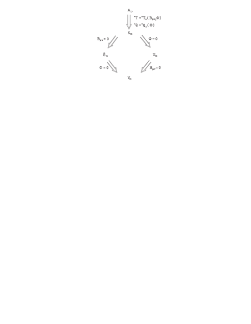
Figure 4: Classification of space-time. $A_{D}$ is affine space-time, $S_{D}$ is stringy space-time, Š_D is stringy torsion free space-time, $U_{D}$ is stringy Riemann-Cartan space-time and $V_{D}$ is Riemann space-time.

All covariant derivatives are defined in the standard way

$${}^{\circ}D_{\mu}V_{\nu}=\partial_{\mu}V_{\nu}-{}^{\circ}\Gamma^{\rho}_{\nu\mu}V_{\rho}\,,\qquad{}^{\circ}D_{\mu}V^{\nu}=\partial_{\mu}V^{\nu}+{}^{\circ}\Gamma^{\nu}_{\rho\mu}V^{\rho}.$$ (195)

The world-sheet is affine C-dual (antidual) surface

$${}^{\circ}H^{i}=\pm{}^{\ast}H^{i}\,\qquad\Longleftrightarrow\qquad\left(G^{\alpha\beta}\mp{\varepsilon^{\alpha\beta}\over\sqrt{-G_{2}}}\right){}^{\circ}\!b^{i}_{\beta\alpha}=0\,.$$ (196)

$\blacktriangleright$ In the Riemann space-time, $V_{D}\equiv(M_{D},\Gamma,G)$, the torsion and nonmetricity vanish ${}^{\circ}T^{\mu}_{\rho\sigma}=0$, ${}^{\circ}Q^{\mu}_{\rho\sigma}=0$, and the connection is just the Christoffel one ${}^{\circ}\Gamma^{\rho}_{\nu\mu}=\Gamma^{\rho}_{\nu\mu}$.

The world-sheet is minimal surface

$$H^{i}\equiv\hbox{${1\over 2}$}G^{\alpha\beta}b^{i}_{\beta\alpha}=0\,.$$ (197)

$\blacktriangleright$ In the stringy Riemann-Cartan space-time, $U_{D}\equiv(M_{D},\Gamma_{\pm},G)$, there are two types of the torsion

$${}^{\circ}T^{\mu}_{\rho\sigma}\to T^{\mu}_{\pm\rho\sigma}=\pm 2B^{\mu}_{\rho\sigma}\,,$$ (198)

where the new term is the field strength of the antisymmetric tensor

$$B_{\mu\nu\rho}=\partial_{\mu}B_{\nu\rho}+\partial_{\nu}B_{\rho\mu}+\partial_{\rho}B_{\mu\nu}=D_{\mu}B_{\nu\rho}+D_{\nu}B_{\rho\mu}+D_{\rho}B_{\mu\nu}\,.$$ (199)

Consequently, there are two types of the connection

$${}^{\circ}\Gamma^{\rho}_{\nu\mu}\to\Gamma^{\rho}_{\pm\nu\mu}=\Gamma^{\rho}_{\nu\mu}\pm B^{\rho}_{\nu\mu}\,,$$ (200)

which can be expressed in terms of the variables $G_{\pm\mu\nu}\equiv\pm 2\Pi_{\pm\mu\nu}=G_{\mu\nu}\pm 2B_{\mu\nu}$

$$\Gamma_{\pm\rho,\nu\mu}=\frac{1}{2}(\partial_{\nu}G_{\pm\mu\rho}+\partial_{\mu}G_{\pm\rho\nu}-\partial_{\rho}G_{\pm\mu\nu})\,,$$ (201)

in the similar way as $\Gamma_{\rho,\nu\mu}$ can be expressed in terms of $G_{\mu\nu}$. The nonmetricity in the stringy Riemann-Cartan space-time vanishes, ${}^{\circ}Q_{\mu\rho\sigma}=0$.

The world-sheet is C-dual (antidual) surface

$$H_{i}=\pm{}^{\ast}H_{\mp i}\,,\qquad\Longleftrightarrow\qquad\left(G^{\alpha\beta}\mp{\varepsilon^{\alpha\beta}\over\sqrt{-G_{2}}}\right)b_{\mp i\beta\alpha}=0\,.$$ (202)

$\blacktriangleright$ In the stringy torsion free space-time, Š${}_{D}\equiv(M_{D},{}^{\star}\Gamma,G)$, the torsion vanishes ${}^{\circ}T^{\mu}_{\rho\sigma}=0$, while the nonmetricity and connection obtain the forms

$${}^{\circ}Q_{\mu\rho\sigma}\to{}^{\star}Q_{\mu\rho\sigma}\equiv-{}^{\star}D_{\mu}G_{\rho\sigma}={1\over a^{2}}D_{\mu}(a_{\rho}a_{\sigma})\,,$$ (203)

and

$${}^{\circ}\Gamma^{\rho}_{\nu\mu}\to{}^{\star}\Gamma^{\rho}_{\nu\mu}=\Gamma^{\rho}_{\nu\mu}+{a^{\rho}\over a^{2}}D_{\mu}a_{\nu}\,.$$ (204)

The world-sheet is stringy minimal surface

$${}^{\star}H_{i}\equiv\hbox{${1\over 2}$}G^{\alpha\beta}\,{}^{\star}b_{i\beta\alpha}=0\,.$$ (205)

$\blacktriangleright$ Finally, in the stringy space-time, $S_{D}\equiv(M_{D},{}^{\star}\Gamma_{\pm},G)$, both the torsion and the nonmetricity survive in the following forms

$${}^{\circ}T^{\rho}_{\mu\nu}\to{}^{\star}T_{\pm}{}^{\rho}_{\mu\nu}=\pm 2P^{T\rho}{}_{\sigma}B^{\sigma}_{\mu\nu}=\pm 2G^{(D-1)\rho}{}_{\sigma}B^{\sigma}_{\mu\nu}\,,$$ (206)

$${}^{\circ}Q_{\mu\rho\sigma}\to{}^{\star}Q_{\pm\mu\rho\sigma}\equiv-{}^{\star}D_{\pm\mu}G_{\rho\sigma}={1\over a^{2}}D_{\pm\mu}(a_{\rho}a_{\sigma})\,,$$ (207)

with the contribution of all three background fields $G_{\mu\nu}$, $B_{\mu\nu}$ and $\Phi$. The stringy connection

$${}^{\circ}\Gamma^{\rho}_{\nu\mu}\to{}^{\star}\Gamma^{\rho}_{\pm\nu\mu}=\Gamma^{\rho}_{\pm\nu\mu}+{a^{\rho}\over a^{2}}D_{\pm\mu}a_{\nu}=P^{T\rho}{}_{\sigma}\Gamma^{\sigma}_{\pm\nu\mu}+{a^{\rho}\over a^{2}}\partial_{\mu}a_{\nu}\,,$$ (208)

has the following symmetry

$${}^{\star}\Gamma^{\rho}_{\pm\nu\mu}={}^{\star}\Gamma^{\rho}_{\mp\mu\nu}\,.$$ (209)

Covariant derivatives of the vector field $a_{\mu}$, have a properties $D_{\pm\mu}a_{\nu}=D_{\mp\nu}a_{\mu}$ and ${}^{\star}D_{\pm\mu}a_{\nu}=0$.

The world-sheet is stringy C-dual (antidual) surface

$${}^{\star}H_{i}=\pm{}^{\ast}H_{\mp i}\,,\qquad\Longleftrightarrow\qquad\left(G^{\alpha\beta}\mp{\varepsilon^{\alpha\beta}\over\sqrt{-G_{2}}}\right){}^{\star}b_{\mp i\beta\alpha}=0\,.$$ (210)