Three-loop $\beta$-function for $N=1$ supersymmetric electrodynamics, regularized by higher derivatives.

Abstract

Three-loop quantum corrections to the effective action are calculated for $N~{}=~{}1$ supersymmetric electrodynamics, regularized by higher derivatives. Using the obtained results we investigate the anomaly puzzle in the considered model.

Moscow State University, Physical Faculty,
Department of Theoretical Physics.
$117234$, Moscow, Russia

1 Introduction.

It is well known [1, 2, 3, 4], that in supersymmetric theories the axial and the trace of the energy-momentum tensor anomalies are components of a chiral scalar supermultiplet. Adler-Bardeen theorem [5, 6] asserts that there are no radiative corrections to the axial anomaly beyond the one-loop approximation, while the trace anomaly is proportional to the $\beta$-function [7] to all orders. Therefore it seems to imply, that the $\beta$-function in supersymmetric theories should be exhausted by the first loop [8]. It does take place in models with $N=2$ supersymmetry [9]. However explicit perturbative calculations find higher order corrections to the $\beta$-functions of $N=1$ supersymmetric theories, regularized by dimensional reduction [10, 11, 12]. This contradiction is usually called ”the anomaly puzzle”.

Many papers were written in the attempt of solving the anomaly puzzle in supersymmetric theories. For example, in [13] the anomaly puzzle is argued to be a consequence of the difference between the usual and Wilsonian effective actions. In particular, the authors noted, that there was a nontrivial contribution to the $\beta$-function related with the Konishi anomaly [14, 15]. The investigation of this contribution in [13] and the investigation of instanton contributions in [16] have led to the construction of the so-called exact Novikov, Shifman, Vainshtein and Zakharov (NSVZ) $\beta$-function. For $N=1$ supersymmetric electrodynamics (SUSY QED) considered in this paper the NSVZ $\beta$-function has the following form:

$$\beta(\alpha)=\frac{\alpha^{2}}{\pi}\Big{(}1-\gamma(\alpha)\Big{)},$$ (1)

where $\gamma(\alpha)$ is the anomalous dimension of the matter superfield. Explicit perturbative calculations with the dimensional reduction (DRED) verify the NVSZ $\beta$-function up to the two-loop order. Nevertheless, the three-loop results obtained in [17, 18, 19] do not agree with the NSVZ $\beta$-function. However [18] this disagreement can be eliminated by a special choice of renormalization scheme, the possibility of such a choice being highly nontrivial [20]. Actually it is possible to relate $\overline{\mbox{DRED}}$ scheme and NSVZ scheme order by order [21] in the perturbation theory. It is worth mentioning, that at two-loops the NSVZ $\beta$-function was also obtained with differential renormalization [22]. For example, for $N=1$ SUSY Yang-Mills the calculation was made in [23].

However the relation between $\Gamma$ and the Wilsonian action remained unclear. This problem was avoided in another solution of the anomaly puzzle, proposed in [24]. The main idea of [24] is that the higher order corrections in NSVZ $\beta$-function are due to anomalous Jacobian under the rescaling of the fields done in passing from holomorphic to canonical normalization. In the case of supersymmetric electrodynamics holomorphic normalization means, that the renormalized action is written as

$$S_{ren}=\frac{1}{4e^{2}}Z_{3}(\Lambda/\mu)\mbox{Re}\int d^{4}x\,d^{2}\theta\,W_{a}C^{ab}W_{b}+$$

$$\qquad\qquad\qquad\qquad\qquad+Z(\Lambda/\mu)\frac{1}{4}\int d^{4}x\,d^{4}\theta\,\Big{(}\phi^{*}e^{2V}\phi+\tilde{\phi}^{*}e^{-2V}\tilde{\phi}\Big{)},\qquad$$ (2)

while in the canonical normalization

$$S_{ren}=\frac{1}{4e^{2}}Z_{3}(\Lambda/\mu)\mbox{Re}\int d^{4}x\,d^{2}\theta\,W_{a}C^{ab}W_{b}+$$

$$\qquad\qquad\qquad\qquad\qquad\qquad\quad+\frac{1}{4}\int d^{4}x\,d^{4}\theta\,\Big{(}\phi^{*}e^{2V}\phi+\tilde{\phi}^{*}e^{-2V}\tilde{\phi}\Big{)}.\qquad$$ (3)

In the former case the $\beta$-function is supposed to be exhausted at the one loop, while in the latter one it coincides with the NVSZ result. In principle this solution is different from the one, given by Shifman and Vainshtein. Moreover, it contradicts the results of explicit two-loop calculations, made with DRED.

It would be natural to suppose, that in the holomorphic normalization the $\beta$-function is exhausted at the one-loop if higher covariant derivative regularization [25, 26], supplemented by the Pauli-Villars, is used. This regularization is known to yield the same result for one-loop logarithmic divergences as the dimensional regularization (or dimensional reduction) [27]. The explicit two-loop calculations for theories, regularized by higher derivatives (HD), were made first in [28, 29] for $N=1$ SUSY QED and gave a zero two-loop contribution to the $\beta$-function defined by

$$\beta(\alpha)=\frac{d}{d\ln\mu}\Bigg{(}\frac{e^{2}}{4\pi}\Bigg{)}.$$ (4)

This result implies the absence of the anomaly puzzle in view of the solution proposed in [24]. However it was not quite clear why different regularizations give different results for the scheme independent two-loop $\beta$-function. Actually in [28] we noted, that the using of the HD regularization leads to a nontrivial contribution of diagrams with insertions of one-loop counterterms, which does not exist for the dimensional reduction. The calculations of this contribution with different regularizations were analysed in [30], where the difference of the results for the scheme independent two-loop $\beta$-function was attributed to the mathematical inconsistency of DRED [31], which had been pointed in [32]. In particular, the inconsistency of DRED leads to incorrect zero results for anomalies, because DRED does not break the chiral symmetry. It is necessary to stress an essential difference between dimensional regularization (DREG) [33] and DRED: DREG allows to derive the axial anomaly unambiguously [33]. However DREG explicitly breaks supersymmetry and is not convenient for the calculations in supersymmetric theories. Let us note, that anomalies can in principle be calculated with DRED. However for this purpose it is necessary to impose mathematically inconsistent conditions like $\mbox{tr}(AB)\neq\mbox{tr}(BA)$ [34] or use some identities between $\gamma$-matrices, which are valid only for $n>4$ [35]. (DRED requires that the space-time dimension $n$ should be less than 4 [31].) However such conditions can not be imposed if the calculations are made by the supergraph technique. Hence the axial anomaly and the Konishi anomaly, calculated with DRED, are equal to 0. As a consequence the additional anomalous contribution, pointed in [13], is omitted if the theory is regularized by DRED. HD regularization is mathematically consistent and allows to calculate anomalies correctly. In particular, the anomalous contribution to the $\beta$-function, obtained with HD, is not equal to 0. Actually this contribution is a sum of Feynman diagrams with insersions of counterterms on matter lines. The sum of such diagrams is equal to 0 with DRED and agrees with the results of [13] and [24] with HD regularization. After rescaling, which converts (1) into (1), the diagrams with insersions of counterterms vanish, and the $\beta$-function becomes equal to the NSVZ expression.

It is necessary to note, that although the $\beta$-function (4) is exausted by the first loop in the holomorphic normalization, the Gell-Mann-Low function has contributions from all orders. This contradiction is discussed in the present paper. We argue, that if the Adler-Bardeen theorem is valid and the bare coupling constant does not depend on $\mu$, then the generating functional depends on $\mu$ due to the rescaling anomaly and $\beta$-function (4) is not related with the Gell-Mann-Low function. Therefore there is no contradiction between the form of the Gell-Mann-Low function and the multiplet structure of anomalies.

One more purpose of this paper is the calculation of the $\beta$-function in the three-loop approximation. It is desirable in order to avoid some possible errors or incorrect interpretation of the results, especially if we take into account, that the three-loop $\beta$-function, considered as a function of $\alpha$, is scheme-dependent. The three-loop contribution to $\beta$-function (4) is found to be 0, and agrees with the predictions of [24] and [30]. It is worth mentioning, that in the three-loop approximation the sum of the diagrams without insersions of counterterms (on matter lines) for a large number of subtraction schemes is equal to the exact $\beta$-function (calculation with DRED gives the NSVZ $\beta$-function only after a redefinition of the coupling constant). The sum of the diagrams with insersions of counterterms in two- and three-loop approximations agrees with the exact expression found in [30], and cancels the other two- and three-loop contributions.

The paper is organized as follows:

In section 2 we consider $N=1$ SUSY QED and regularize it by higher derivatives. The three-loop $\beta$-function and its relation with two-loop anomalous dimension are analysed in section 3. In particular, the three-loop contribution to the $\beta$-function is found to be 0. In section 4 we explain why the results are different from those obtained with DRED. The anomaly puzzle is considered in section 5. Section 6 contains some concluding remarks. The details of the calculations are presented in appendixes. Appendix A contains expressions for various groups of Feynman diagrams. The calculations of the corresponding contributions are made in appendix B and the most useful three-loop integrals are analysed in appendix C.

2 $N=1$ supersymmetric electrodynamics and higher derivative regularization.

$N=1$ supersymmetric electrodynamics is described by the following action:

$$S_{0}=\frac{1}{4e^{2}}\mbox{Re}\int d^{4}x\,d^{2}\theta\,W_{a}C^{ab}W_{b}+\frac{1}{4}\int d^{4}x\,d^{4}\theta\,\Big{(}\phi^{*}e^{2V}\phi+\tilde{\phi}^{*}e^{-2V}\tilde{\phi}\Big{)}.$$ (5)

Here $\phi$ and $\tilde{\phi}$ are chiral superfields

$$\phi(y,\theta)=\varphi(y)+\bar{\theta}(1+\gamma_{5})\psi(y)+\frac{1}{2}\bar{\theta}(1+\gamma_{5})\theta f(y);$$

$$\tilde{\phi}(y,\theta)=\tilde{\varphi}(y)+\bar{\theta}(1+\gamma_{5})\tilde{\psi}(y)+\frac{1}{2}\bar{\theta}(1+\gamma_{5})\theta\tilde{f}(y),$$ (6)

where $y^{\mu}=x^{\mu}+i\bar{\theta}\gamma^{\mu}\gamma_{5}\theta/2$. Two Majorana spinors $\psi$ and $\tilde{\psi}$ form one Dirac spinor

$$\Psi=\frac{1}{\sqrt{2}}\Big{(}(1+\gamma_{5})\psi+(1-\gamma_{5})\tilde{\psi}\Big{)}.$$ (7)

$V$ in (5) is a real superfield

$$V(x,\theta)=C(x)+i\sqrt{2}\bar{\theta}\gamma_{5}\xi(x)+\frac{1}{2}(\bar{\theta}\theta)K(x)+\frac{i}{2}(\bar{\theta}\gamma_{5}\theta)H(x)+\frac{1}{2}(\bar{\theta}\gamma^{\mu}\gamma_{5}\theta)A_{\mu}(x)+$$

$$+\sqrt{2}(\bar{\theta}\theta)\bar{\theta}\Big{(}i\gamma_{5}\chi(x)+\frac{1}{2}\gamma^{\mu}\gamma_{5}\partial_{\mu}\xi(x)\Big{)}+\frac{1}{4}(\bar{\theta}\theta)^{2}\Big{(}D(x)-\frac{1}{2}\partial^{2}C(x)\Big{)},$$ (8)

where, in particular, $A_{\mu}$ is an Abelian gauge field. The superfield $W_{a}$ in the Abelian case is defined by

$$W_{a}=\frac{1}{16}\bar{D}(1-\gamma_{5})D\Big{[}(1+\gamma_{5})D_{a}V\Big{]},$$ (9)

where

$$D=\frac{\partial}{\partial\bar{\theta}}-i\gamma^{\mu}\theta\,\partial_{\mu}$$ (10)

is a supersymmetric covariant derivative.

In order to regularize model (5) by HD its action should be modified as follows:

$$S_{0}\to S=S_{0}+S_{\Lambda}=\vphantom{\frac{1}{2}}$$

$$\qquad=\frac{1}{4e^{2}}\mbox{Re}\int d^{4}x\,d^{2}\theta\,W_{a}C^{ab}\Big{(}1+\frac{\partial^{2n}}{\Lambda^{2n}}\Big{)}W_{b}+$$

$$\qquad\qquad\qquad\qquad\qquad\qquad+\frac{1}{4}\int d^{4}x\,d^{4}\theta\,\Big{(}\phi^{*}e^{2V}\phi+\tilde{\phi}^{*}e^{-2V}\tilde{\phi}\Big{)}.\qquad$$ (11)

Note, that in the Abelian case the superfield $W^{a}$ is gauge invariant, so the higher derivative term contains usual derivatives.

The quantization of (2) can be made by using standard technique described in [36] and is not considered here. It only needs mentioning that the gauge invariance was fixed by adding

$$S_{gf}=-\frac{1}{64e^{2}}\int d^{4}x\,d^{4}\theta\,\Bigg{(}VD^{2}\bar{D}^{2}\Big{(}1+\frac{\partial^{2n}}{\Lambda^{2n}}\Big{)}V+V\bar{D}^{2}D^{2}\Big{(}1+\frac{\partial^{2n}}{\Lambda^{2n}}\Big{)}V\Bigg{)},$$ (12)

where

$$D^{2}\equiv\frac{1}{2}\bar{D}(1+\gamma_{5})D;\qquad\bar{D}^{2}\equiv\frac{1}{2}\bar{D}(1-\gamma_{5})D.$$ (13)

After adding such terms the free part of the action for the superfield $V$ is written in the simplest form

$$S_{gauge}+S_{gf}=\frac{1}{4e^{2}}\int d^{4}x\,d^{4}\theta\,V\partial^{2}\Big{(}1+\frac{\partial^{2n}}{\Lambda^{2n}}\Big{)}V.$$ (14)

In the Abelian case diagrams containing ghost loops are missing.

The superficial degree of divergence for the model (2) is (see e.f. [28])

$$\omega_{\Lambda}=2-2n(L-1)-E_{\phi}(n+1),$$ (15)

where $L$ is a number of loops and $E_{\phi}$ is a number of external $\phi$-lines. According to (15) divergences remain in one-loop diagrams even for $n\geq 2$. In order to regularize these divergences it is necessary to insert Pauli-Villars determinants [6] into the generating functional. Due to the supersymmetric gauge invariance

$$V\to V-\frac{1}{2}(A+A^{+});\qquad\phi\to e^{A}\phi;\qquad\tilde{\phi}\to e^{-A}\tilde{\phi},$$ (16)

where $A$ is an arbitrary chiral scalar superfield, the renormalized action can be written as

$$S_{ren}=\frac{1}{4e^{2}}Z_{3}(\Lambda/\mu)\mbox{Re}\int d^{4}x\,d^{2}\theta\,W_{a}C^{ab}\Big{(}1+\frac{\partial^{2n}}{\Lambda^{2n}}\Big{)}W_{b}+$$

$$\qquad\qquad\qquad\qquad\qquad+Z(\Lambda/\mu)\frac{1}{4}\int d^{4}x\,d^{4}\theta\,\Big{(}\phi^{*}e^{2V}\phi+\tilde{\phi}^{*}e^{-2V}\tilde{\phi}\Big{)}.\qquad$$ (17)

Hence the generating functional is

$$Z=\int DV\,D\phi\,D\tilde{\phi}\,\prod\limits_{i}\Big{(}\det PV(V,M_{i})\Big{)}^{c_{i}}\exp\Bigg{\{}i\Bigg{[}\frac{1}{4e^{2}}\int d^{4}x\,d^{4}\theta\,V\partial^{2}\Big{(}1+\frac{\partial^{2n}}{\Lambda^{2n}}\Big{)}V-$$

$$-\frac{1}{4e^{2}}\Big{(}Z_{3}(\Lambda/\mu)-1\Big{)}\int d^{4}x\,d^{4}\theta\,V\Pi_{1/2}\partial^{2}\Big{(}1+\frac{\partial^{2n}}{\Lambda^{2n}}\Big{)}V+$$

$$\qquad\qquad\qquad\qquad\qquad\qquad\qquad\qquad+\frac{1}{4}Z(\Lambda/\mu)\int d^{4}x\,d^{4}\theta\,\Big{(}\phi^{*}e^{2V}\phi+\tilde{\phi}^{*}e^{-2V}\tilde{\phi}\Big{)}+$$

$$+\int d^{4}x\,d^{4}\theta\,JV+\int d^{4}x\,d^{2}\theta\,\Big{(}j\,\phi+\tilde{j}\,\tilde{\phi}\Big{)}+\int d^{4}x\,d^{2}\bar{\theta}\,\Big{(}j^{*}\phi^{*}+\tilde{j}^{*}\tilde{\phi}^{*}\Big{)}\Bigg{]}\Bigg{\}},$$ (18)

where

$$\Big{(}\det PV(V,M)\Big{)}^{-1}=\int D\Phi\,D\tilde{\Phi}\,\exp\Bigg{\{}i\Bigg{[}Z(\Lambda/\mu)\frac{1}{4}\int d^{4}x\,d^{4}\theta\,\Big{(}\Phi^{*}e^{2V}\Phi+\qquad$$

$$+\tilde{\Phi}^{*}e^{-2V}\tilde{\Phi}\Big{)}+\frac{1}{2}\int d^{4}x\,d^{2}\theta\,M\tilde{\Phi}\Phi+\frac{1}{2}\int d^{4}x\,d^{2}\bar{\theta}\,M\tilde{\Phi}^{*}\Phi^{*}\Bigg{]}\Bigg{\}},$$ (19)

and the coefficients $c_{i}$ satisfy equations

$$\sum\limits_{i}c_{i}=1;\qquad\sum\limits_{i}c_{i}M_{i}^{2}=0.$$ (20)

Below we assume, that $M_{i}=a_{i}\Lambda$, where $a_{i}$ are some constants. The insertion of Pauli-Villars determinants allows us to cancel remaining divergences in all one-loop diagrams, including diagrams with insertions of counterterms. Later we will show, that the divergencies in the sum of two- and three-loop diagrams with Pauli-Villars loops cancel each other. Therefore, for diagrams with loops of Pauli-Villars fields it is unnecessary to introduce any other regularization.

In our notations the generating functional for connected Green functions is defined by

$$W=-i\ln Z,$$ (21)

and an effective action is obtained by making a Legendre transformation:

$$\Gamma=W-\int d^{4}x\,d^{4}\theta\,JV-\int d^{4}x\,d^{2}\theta\,\Big{(}j\,\phi+\tilde{j}\,\tilde{\phi}\Big{)}-\int d^{4}x\,d^{2}\bar{\theta}\,\Big{(}j^{*}\phi^{*}+\tilde{j}^{*}\tilde{\phi}^{*}\Big{)},$$ (22)

where $J$, $j$ and $\tilde{j}$ is to be eliminated in terms of $V$, $\phi$ and $\tilde{\phi}$, through solving equations

$$V=\frac{\delta W}{\delta J};\qquad\phi=\frac{\delta W}{\delta j};\qquad\tilde{\phi}=\frac{\delta W}{\delta\tilde{j}}.$$ (23)

After obtaining $S_{ren}$, it is possible to find the $\beta$-function and the anomalous dimension, which in our notations are defined by

$$\beta=\frac{d}{d\ln\mu}\Bigg{(}\frac{e^{2}}{4\pi}\Bigg{)};\qquad\quad\gamma=\frac{d\ln Z}{d\ln\mu}.$$ (24)

(We assume, that the bare coupling constant $e_{0}$, defined by

$$\frac{1}{e_{0}^{2}}=\frac{1}{e^{2}}Z_{3}(\Lambda/\mu),$$ (25)

does not depend on $\mu$. Hence the renormalized coupling constant $e$ depends on $\mu$.) It is easy to see [7], that the trace anomaly is proportional to $\beta$-function (24).

The $\beta$-function and anomalous dimension, given by (24), which are considered as functions of $e$, are changed at the simultanious redefinition of the renormalized coupling $e$ and the renormalization constant $Z_{3}$, provided $e_{0}=\mbox{const}$. In other words they depend on the renormalization scheme. If $\beta$ and $\gamma$ are expanded in powers of $e^{2}$, then the coefficients of the $\beta$-function and anomalous dimension become scheme-dependent starting from the three- and two-loop approximation respectively.

Note, that it is possible to use another definition of the $\beta$-function. Let us consider transversal part of the two-point Green function for the gauge field:

$$\Pi_{1/2}\,\int d^{4}x\,d^{4}y\,\frac{\delta^{2}\Gamma}{\delta V_{x}\,\delta V_{y}}\Bigg{|}_{J=0}\exp\Big{(}ip_{\mu}x^{\mu}+iq_{\mu}y^{\mu}\Big{)}=$$

$$\qquad\qquad\qquad\qquad=\frac{1}{8\pi}(2\pi)^{4}\delta^{4}\Big{(}p+q\Big{)}\,p^{2}\Pi_{1/2}\delta^{4}(\theta_{x}-\theta_{y})\,d^{-1}(\alpha,\mu/p),\qquad$$ (26)

where

$$\Pi_{1/2}\equiv-\frac{1}{16\partial^{2}}D^{a}\bar{D}^{2}C_{ab}D^{b}.$$ (27)

Then it is possible to define Gell-Mann-Low function

$$\tilde{\beta}\Big{(}d(\alpha,x)\Big{)}\equiv-x\frac{\partial}{\partial x}d(\alpha,x).$$ (28)

Taking into account, that the effective action should not depend on the normalization point $\mu$ and differentiating equation (2) over $\ln\mu$ we obtain

$$0=\tilde{\beta}\Big{(}d(\alpha,x)\Big{)}-\beta(\alpha)\frac{\partial}{\partial\alpha}d(\alpha,x).$$ (29)

In particular at $x=1$ we have

$$\tilde{\beta}(\tilde{\alpha})=\beta(\alpha)\frac{d\tilde{\alpha}}{d\alpha},$$ (30)

where $\tilde{\alpha}\equiv d(\alpha,1)$. Therefore, if the generating functional does not depend on $\mu$, then both definitions of the $\beta$-function are equivalent.

In order to find the $\beta$-function and the anomalous dimension it is necessary to calculate all 1PI graphs in the considered approximation. The expressions for them are constructed in accordance with Feynman rules, which can be formulated as follows:

1. External lines give the integration

$$\prod\limits_{E}\int\frac{d^{4}p_{{}_{E_{V}}}}{(2\pi)^{4}}V(p_{{}_{E_{V}}})\int\frac{d^{4}p_{{}_{E_{\phi}}}}{(2\pi)^{4}}\phi(p_{{}_{E_{\phi}}})\cdot\ldots\cdot(2\pi)^{4}\delta\Big{(}\sum\limits_{E}p_{{}_{E}}\Big{)},$$ (31)

where $E$ runs over external momenta.

2. Propagator of the superfield $V$ is

$$\frac{8e^{2}}{(k^{2}+i0)\Big{(}1+(-1)^{n}k^{2n}/\Lambda^{2n}\Big{)}}\,\delta^{4}(\theta_{1}-\theta_{2}).$$ (32)

3. Massless $\phi-\phi^{*}$ and $\tilde{\phi}-\tilde{\phi}^{*}$ propagators are

$$-\frac{1}{16(k^{2}+i0)}\bar{D}^{2}D^{2}\delta^{4}(\theta_{1}-\theta_{2}).$$ (33)

(Note that the considered action is quadratic in matter superfields and Feynman rules can be simplified in comparison with, say, Wess-Zumino model.)

4. Pauli-Villars fields are present only in the closed loops. Each internal line $\Phi-\Phi^{*}$ or $\tilde{\Phi}-\tilde{\Phi}^{*}$ corresponds to

$$-\frac{1}{16(k^{2}-M_{i}^{2}+i0)}\,\bar{D}^{2}D^{2}\delta^{4}(\theta_{1}-\theta_{2}),$$ (34)

and each internal line $\Phi-\tilde{\Phi}$ or $\Phi^{*}-\tilde{\Phi}^{*}$ – to

$$\frac{M_{i}}{4(k^{2}-M_{i}^{2}+i0)}\,\bar{D}^{2}\delta^{4}(\theta_{1}-\theta_{2})\quad\mbox{and}\quad\frac{M_{i}}{4(k^{2}-M_{i}^{2}+i0)}\,D^{2}\delta^{4}(\theta_{1}-\theta_{2})$$ (35)

respectively. For each loop of Pauli-Villars fields it is necessary to introduce ${\displaystyle-\sum\limits_{i}c_{i}}$.

5. Each loop yields an integration over a loop momentum ${\displaystyle\int\frac{d^{4}k}{(2\pi)^{4}}}$.

6. Each vertex gives ${\displaystyle\int d^{4}\theta}$.

7. There are usual combinatoric factors, which can be found from the generating functional (2).

3 Three-loop $\beta$-function.

The diagrams contributing to the three-loop $\beta$-function are presented in Fig. 1 – 8. Note, that each internal matter loop in these diagrams can correspond to $\phi$ and $\tilde{\phi}$ fields or to Pauli-Villars fields. We devided Feynman diagrams into some groups and presented the expressions for all these groups in appendix A. Then the three-loop correction to the effective action can be written as

$$\Delta\Gamma^{(3)}_{V}=\mbox{Re}\int d^{2}\theta\,\frac{d^{4}p}{(2\pi)^{4}}W_{a}(p)C^{ab}W_{b}(-p)\times$$

$$\qquad\qquad\times\Big{(}f_{1-loop}+f_{O}+f_{O_{PV}}+f_{Oo}+f_{Oo_{PV}}+f_{OO}+f_{XX}+f_{X}+f_{X2}\Big{)},\qquad$$ (36)

where

$f_{1-loop}$ is a contribution of one-loop diagrams, presented in Fig. 1;

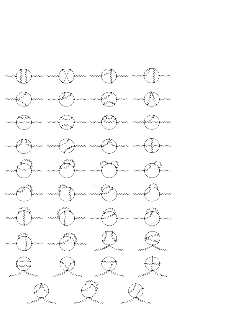
Figure 5: Three-loop graphs with a single loop of matter superfield.

$f_{O}$ is a contribution of diagrams, presented in Fig. 5, containing a single loop of the superfields $\phi$ and $\tilde{\phi}$;

$f_{O_{PV}}$ is a contribution of the same diagrams, having a loop of Pauli-Villars fields;

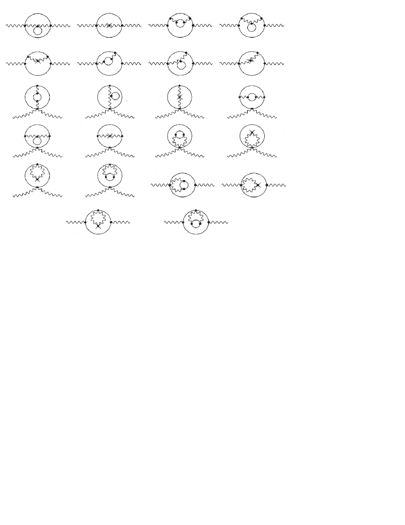
Figure 4: Contribution to $\Delta\Gamma_{V}$, corresponding to corrections to the photon propagator.

$f_{Oo}$ is a contribution of the two-loop diagrams, presented in Fig. 2 (without Pauli-Villars fields) and the three-loop diagrams, presented in Fig. 4, which contain an internal loop of matter superfields or an insersion of one-loop counterterms on the photon line and external loop of $\phi$ and $\tilde{\phi}$ superfields;

$f_{Oo_{PV}}$ is a contribution of the same diagrams with the external loop of Pauli-Villars fields.

$f_{OO}$ is a contribution of the other diagrams with two loops of the matter superfields, presented in Fig. 3;

$f_{X}$ is a contribution of diagrams with an insersion of two-loop counterterms, presented in Fig. 6;

$f_{XX}$ is a contribution of diagrams with two insersions of one-loop counterterms, presented in Fig. 8;

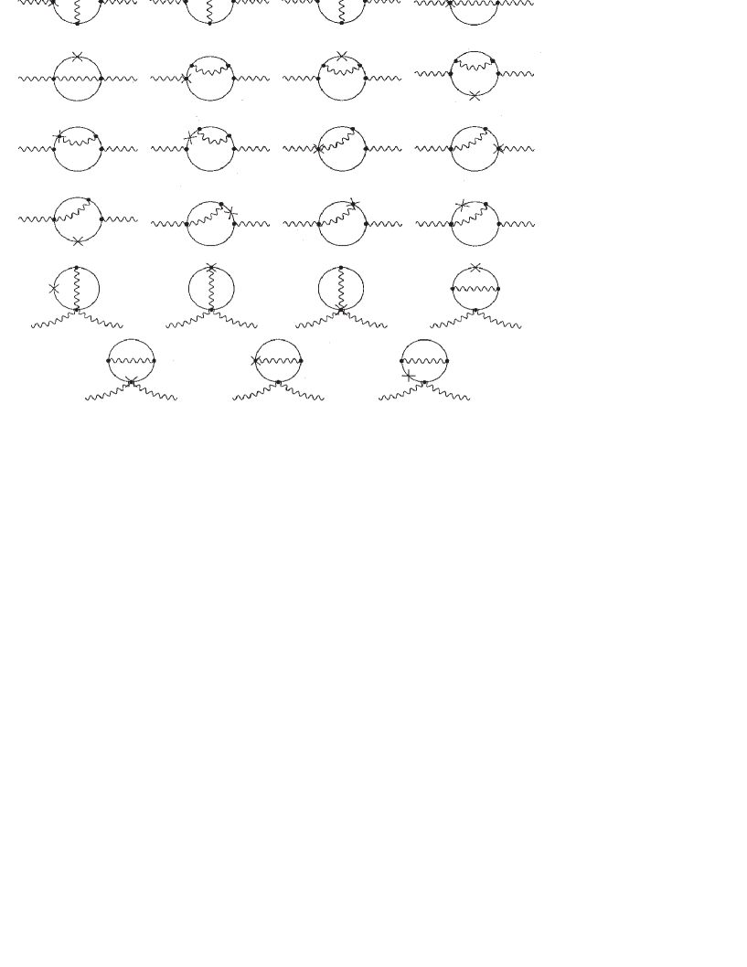
Figure 7: Diagrams containing an insersion of one-loop counterterms.

$f_{X2}$ is a contribution of diagrams with an insersion of one-loop counterterms, presented in Fig. 7.

The explicit expressions for all these contributions were found by means of calculating of the corresponding Feynman diagrams. To check correctness of these calculations we verified the cancellation of noninvariant terms, proportional to

$$\int\frac{d^{4}p}{(2\pi)^{4}}\,d^{4}\theta\,V(p,\theta)\,V(-p,\theta).$$ (37)

The results, presented in appendix A, are analysed in appendix B. Let us briefly discuss them:

1. $f_{OO}=0$, because the substitution $\phi\leftrightarrow\tilde{\phi}$ in a loop changes the sign of a diagram. Indeed, in this case the diagrams, having the same superfields in both loops ($\phi$ and $\phi$ or $\tilde{\phi}$ and $\tilde{\phi}$), are cancelled by diagrams with loops of different superfields ($\phi$ and $\tilde{\phi}$). For the diagrams with Pauli-Villars fields the result is the same, but its derivation is more complicated.

2. The sum of $f_{XX}$, $f_{X}$ and $f_{X2}$ agrees with the exact expression for the sum of diagrams with insersions of counterterms

$$-\ln Z\,\frac{1}{16\pi^{2}}\,\mbox{Re}\int d^{4}x\,d^{2}\theta\,W_{a}C^{ab}W_{b}+\mbox{finite terms},$$ (38)

found in [30]. The corresponding contribution to $\beta$-function in the considered approximation is

$$\Delta\beta=\frac{\alpha^{2}}{\pi}\gamma(\alpha).$$ (39)

According to the results of the one-loop calculations and the predictions of the renormgroup (see e.f. [28]) the constant $Z$ is given by

$$Z(\Lambda/\mu)=1+\frac{\alpha}{\pi}\,\Big{(}\ln\frac{\Lambda}{\mu}+g_{1}\Big{)}+$$

$$\qquad\qquad+\frac{\alpha^{2}}{\pi^{2}}\,\Big{(}\ln^{2}\frac{\Lambda}{\mu}+g_{1}\ln\frac{\Lambda}{\mu}\Big{)}-\gamma_{2}\,\alpha^{2}\,\Big{(}\ln\frac{\Lambda}{\mu}+g_{2}\Big{)}+O(\alpha^{3}).\qquad$$ (40)

Here $\gamma_{2}\alpha^{2}$ is a two-loop contribution to the anomalous dimension and we assume, that at the one-loop the counterterms are

$$\Delta S=-\frac{1}{16\pi^{2}}\Big{(}\ln\frac{\Lambda}{\mu}+b_{1}\Big{)}\mbox{Re}\int d^{4}x\,d^{2}\theta\,W_{a}C^{ab}\Big{(}1+\frac{\partial^{2n}}{\Lambda^{2n}}\Big{)}W_{b}+$$

$$\qquad\qquad\qquad\qquad\qquad+\frac{e^{2}}{16\pi^{2}}\Big{(}\ln\frac{\Lambda}{\mu}+g_{1}\Big{)}\int d^{4}x\,d^{4}\theta\,\Big{(}\phi^{*}e^{2V}\phi+\tilde{\phi}^{*}e^{-2V}\tilde{\phi}\Big{)},\qquad$$ (41)

where $b_{1}$, $g_{1}$ and $g_{2}$ are arbitrary finite constants, which define a subtraction scheme.

3. $f_{Oo_{PV}}$ and $f_{O_{PV}}$ are finite and do not contribute to the divergent part of the effective action. This means, that the sum of all diagrams with Pauli-Villars loops is finite, although there are divergences in some of such graphs. However, Pauli-Villars regularization always assumes the existance of divergent diagrams and the cancellation of the divergences between different graphs. Therefore, in the considered case it is not necessary to introduce any more regularization.

4. The analysis of $f_{Oo}$ and $f_{O}$ is rather involved, because the corresponding integrals are very complicated. Each of these integrals depends on $\Lambda/p$ and is the sum of a third degree polynomial in $\ln\Lambda/p$ and a function, finite at $\Lambda\to\infty$ (or equivalently at $p\to 0$)

$$f(\Lambda/p)=f_{3}\ln^{3}\frac{\Lambda}{p}+f_{2}\ln^{2}\frac{\Lambda}{p}+f_{1}\ln\frac{\Lambda}{p}+f_{0}+o(1).$$ (42)

Let us assume, that the limit

$$\Lambda\frac{d}{d\Lambda}f(\Lambda/p)\Bigg{|}_{p=0}$$ (43)

exists. Then $f_{3}=0$ and $f_{2}=0$, while the considered limit is $f_{1}$.

In appendix B we prove, that for $f_{Oo}$ and $f_{O}$ the limit (43) exists and

$$\Lambda\frac{d}{d\Lambda}\Big{(}f_{Oo}+f_{O}\Big{)}\Bigg{|}_{p=0}=\frac{1}{16\pi^{2}}\Lambda\frac{d}{d\Lambda}\Big{(}z_{1}+z_{2}+\frac{1}{2}z_{1}^{2}\Big{)}\Bigg{|}_{p=0},$$ (44)

where

$$z_{1}\equiv\int\frac{d^{4}k}{(2\pi)^{4}}\,\frac{2e^{2}}{k^{2}(k+p)^{2}\Big{(}1+k^{2n}/\Lambda^{2n}\Big{)}};$$ (45)

$$z_{2}\equiv-\int\frac{d^{4}k}{(2\pi)^{4}}\,\frac{d^{4}l}{(2\pi)^{4}}\,\frac{4e^{4}}{k^{2}l^{2}(k+p)^{2}(l+p)^{2}\Big{(}1+k^{2n}/\Lambda^{2n}\Big{)}\Big{(}1+l^{2n}/\Lambda^{2n}\Big{)}}-$$

$$-\int\frac{d^{4}k}{(2\pi)^{4}}\,\frac{d^{4}l}{(2\pi)^{4}}\,\frac{4e^{4}}{\displaystyle k^{2}l^{2}(l+p)^{2}(k+l+p)^{2}\Big{(}1+k^{2n}/\Lambda^{2n}\Big{)}\Big{(}1+l^{2n}/\Lambda^{2n}\Big{)}}+$$

$$+\int\frac{d^{4}k}{(2\pi)^{4}}\,\frac{d^{4}l}{(2\pi)^{4}}\,\frac{4e^{4}(k+l+2p)^{2}}{k^{2}(k+p)^{2}l^{2}(l+p)^{2}(k+l+p)^{2}\Big{(}1+k^{2n}/\Lambda^{2n}\Big{)}\Big{(}1+l^{2n}/\Lambda^{2n}\Big{)}}-\quad$$

$$-\int\frac{d^{4}k}{(2\pi)^{4}}\,\frac{4e^{4}}{k^{2}(k+p)^{2}\Big{(}1+k^{2n}/\Lambda^{2n}\Big{)}^{2}}\Bigg{(}\int\frac{d^{4}l}{(2\pi)^{4}}\,\frac{1}{l^{2}(k+l)^{2}}-$$ (46)

$$-\sum\limits_{i}c_{i}\int\frac{d^{4}l}{(2\pi)^{4}}\,\frac{1}{(l^{2}+M_{i}^{2})\Big{(}(k+l)^{2}+M_{i}^{2}\Big{)}}-\frac{1}{8\pi^{2}}\Big{(}\ln\frac{\Lambda}{\mu}+b_{1}\Big{)}\Big{(}1+k^{2n}/\Lambda^{2n}\Big{)}\Bigg{)}.\qquad$$

From (44), (45) and (3) we see, that the integral over three loop momenta is reduced to the integral over two loop momenta. It is very nontrivial, that can be seen from the calculations, done in appendixes B and C. In our opinion these facts confirm the correctness of the obtained results.

Note, that $z_{1}$ and $z_{2}$ are present in the two-loop two-point Green function for the matter superfield [29]:

$$\Gamma^{(2)}_{\phi}=\frac{1}{4}\int d^{4}\theta\,\frac{d^{4}p}{(2\pi)^{4}}\,\Big{(}\phi^{*}(p,\theta)\,\phi(-p,\theta)+\tilde{\phi}^{*}(p,\theta)\,\tilde{\phi}(-p,\theta)\Big{)}\Bigg{\{}1-z_{1}-z_{2}-\qquad$$

$$-\frac{e^{2}}{4\pi^{2}}z_{1}\Big{(}\ln\frac{\Lambda}{\mu}+g_{1}\Big{)}+\frac{e^{2}}{4\pi^{2}}\Big{(}\ln\frac{\Lambda}{\mu}+g_{1}\Big{)}+\mbox{two-loop counterterms}\Bigg{\}}.$$ (47)

This expression can be formally written as

$$\Gamma^{(2)}_{\phi}=\frac{1}{4}\int d^{4}\theta\,\frac{d^{4}p}{(2\pi)^{4}}\,\Big{(}\phi^{*}(p,\theta)\,\phi(-p,\theta)+\tilde{\phi}^{*}(p,\theta)\,\tilde{\phi}(-p,\theta)\Big{)}\times$$

$$\qquad\qquad\qquad\qquad\quad\times\Bigg{\{}1-z_{1}-z_{2}-\hat{\Delta}z_{1}\,z_{1}+\hat{\Delta}z_{1}+\hat{\Delta}z_{2}+\hat{\Delta}\Big{(}\hat{\Delta}z_{1}\,z_{1}\Big{)}\Bigg{\}},\qquad$$ (48)

where the operator $\hat{\Delta}$ is constructed as follows: If $f$ is a function of $\Lambda/p$ and $\Lambda/\mu$, then by definition $\hat{\Delta}f$ is a counterterm, which cancels a divergence of the function $f$. For example,

$$\hat{\Delta}z_{1}=\frac{\alpha}{\pi}\Big{(}\ln\frac{\Lambda}{\mu}+g_{1}\Big{)}.$$ (49)

Below we will assume, that the operator $\hat{\Delta}$ is linear. (In a general case this operator can be nonlinear).

From (3) we see, that the two-loop renormalization constant for the matter superfield is given by

$$Z=1+\hat{\Delta}z_{1}+\hat{\Delta}z_{2}+\hat{\Delta}(\hat{\Delta}z_{1}\,z_{1})+O(\alpha^{3}),$$ (50)

so that

$$\ln Z=\hat{\Delta}z_{1}+\hat{\Delta}z_{2}+\hat{\Delta}(\hat{\Delta}z_{1}\,z_{1})-\frac{1}{2}\Big{(}\hat{\Delta}z_{1}\Big{)}^{2}+O(\alpha^{3})=\hat{\Delta}z_{1}+\hat{\Delta}z_{2}-$$

$$-\frac{1}{2}\hat{\Delta}\Big{(}z_{1}-\hat{\Delta}z_{1}\Big{)}^{2}+\frac{1}{2}\hat{\Delta}\Big{(}z_{1}^{2}\Big{)}+\frac{1}{2}\hat{\Delta}\Big{(}(\hat{\Delta}z_{1})^{2}\Big{)}-\frac{1}{2}(\hat{\Delta}z_{1})^{2}+O(\alpha^{3}).\qquad$$ (51)

Taking into account, that due to the definition of $\hat{\Delta}$ the expressions $(z_{1}-\hat{\Delta}z_{1})^{2}$ and $\hat{\Delta}\Big{(}(\hat{\Delta}z_{1})^{2}\Big{)}-(\hat{\Delta}z_{1})^{2}$ are finite, $\ln Z$ can be presented as

$$\ln Z=\hat{\Delta}\Big{(}z_{1}+z_{2}+\frac{1}{2}z_{1}^{2}\Big{)}+\mbox{finite terms}.$$ (52)

Then the sum of diagrams, defining two- and three-loop contributions to the $\beta$-function for $N=1$ SUSY QED, for subtraction schemes, corresponding to any linear operator $\hat{\Delta}$ can be written in the following form:

$$\Delta\Gamma^{(3)}_{V}=\frac{1}{16\pi^{2}}\mbox{Re}\int d^{2}\theta\,\frac{d^{4}p}{(2\pi)^{4}}W_{a}(p)C^{ab}W_{b}(-p)\times$$

$$\qquad\qquad\qquad\times\Bigg{(}z_{1}+z_{2}+\frac{1}{2}z_{1}^{2}-\hat{\Delta}\Big{(}z_{1}+z_{2}+\frac{1}{2}z_{1}^{2}\Big{)}+\mbox{finite terms}\Bigg{)}.\qquad$$ (53)

This expression is finite due to the definition of $\hat{\Delta}$, so it is not necessary to add any counterterms in two- and three-loop approximations. Thus for all renomalization schemes with linear $\hat{\Delta}$ we have:

$$\frac{4\pi^{2}}{e_{0}^{2}}=\frac{\pi}{\alpha\Big{(}\Lambda/\mu\Big{)}}-\ln\frac{\Lambda}{\mu}-b_{1}+O(\alpha^{3}).$$ (54)

This means, that the two- and three-loop contributions to the $\beta$-function are equal to zero and

$$\beta=\frac{\alpha^{2}}{\pi}+O(\alpha^{5}).$$ (55)

Hence the $\beta$-function is exhausted at the one-loop and agrees with the multiplet structure of anomalies.

Note, that the sum of diagrams which do not contain insersions of counterterms on matter lines in the considered approximation gives the following contribution to the $\beta$-function:

$$\Delta\beta=\frac{\alpha^{2}}{\pi}\Big{(}1-\gamma(\alpha)\Big{)}.$$ (56)

This contribution is equal to the NSVZ $\beta$-function, but the anomalous dimension is cancelled after adding (39), and the final result is comletely defined by the one-loop.

4 Comparison between HD regularization and DRED.

The $\beta$-function obtained in the previous section is different from the corresponding result, found with DRED. In the two-loop approximation the calculations of the effective action with DRED and HD were compared in [30]. The difference of the results for the $\beta$-function is shown to have originated from the different results for the sum of diagrams with insersions of counterterms. With DRED this contribution is 0, while with HD it is given by (38). The calculations made in this paper show, that in the three-loop approximation we have a similar situation.

The difference of the results for the sum of diagrams with insersions of counterterms [30] is caused by the mathematical inconsistancy of DRED, pointed in [32], because this inconsistency leads to zero results for all anomalies. (We assume, that there are no assumptions like $\mbox{tr}(AB)\neq\mbox{tr}(BA)$ and all identities are valid for $n<4$.) In particular the sum of diagrams with insersions of counterterms on the matter lines calculated with DRED is 0.

Let us discuss this in detail:

In supersymmetric theories the axial anomaly is related with the Konishi anomaly [14, 15]. Indeed, let us consider

$$\mbox{Im}\Bigg{[}\bar{D}^{2}\Big{(}\phi^{*}e^{2V}\phi+\tilde{\phi}^{*}e^{-2V}\tilde{\phi}\Big{)}\Bigg{]}.$$ (57)

Using equations (2) and (2), it is easy to see, that in components this expression will contain (among other terms)

$$-\bar{\theta}\theta\,\partial_{\mu}\Big{(}\bar{\Psi}\gamma^{\mu}\gamma_{5}\Psi\Big{)},$$ (58)

where the Dirac spinor $\Psi$ is defined by (7). It is well known [37], that the conservation of the axial current is broken by quantum corrections and in particular

$$\bar{\theta}\theta\,\langle\partial_{\mu}\Big{(}\bar{\Psi}\gamma^{\mu}\gamma_{5}\Psi\Big{)}\rangle=-\bar{\theta}\theta\,\frac{1}{8\pi^{2}}F_{\mu\nu}\tilde{F}^{\mu\nu}.$$ (59)

Hence due to the supersymmetry

$$\mbox{Im}\,\Big{\langle}\bar{D}^{2}\Big{(}\phi^{*}e^{2V}\phi+\tilde{\phi}^{*}e^{-2V}\tilde{\phi}\Big{)}\Big{\rangle}=\frac{1}{2\pi^{2}}\mbox{Im}\Big{(}W_{a}C^{ab}W_{b}\Big{)}.$$ (60)

By performing supersymmetry transformations it is easy to see, that if an imaginary part of a chiral superfield is equal to 0, then this superfield is a real constant. Therefore, from (60) we obtain, that

$$\Big{\langle}\bar{D}^{2}\Big{(}\phi^{*}e^{2V}\phi+\tilde{\phi}^{*}e^{-2V}\tilde{\phi}\Big{)}\Big{\rangle}=\frac{1}{2\pi^{2}}W_{a}C^{ab}W_{b}+\mbox{const}.$$ (61)

Applying

$$-\frac{1}{2}\int d^{4}x\,D^{2}=\int d^{4}x\,d^{2}\theta$$ (62)

to (61) and taking a real part of the result, we obtain, that

$$\Big{\langle}\frac{1}{4}\int d^{4}x\,d^{4}\theta\,\Big{(}\phi^{*}e^{2V}\phi+\tilde{\phi}^{*}e^{-2V}\tilde{\phi}\Big{)}\Big{\rangle}=-\frac{1}{16\pi^{2}}\mbox{Re}\int d^{4}x\,d^{2}\theta\,W_{a}C^{ab}W_{b}.$$ (63)

Because DRED requires, that the space-time dimension $n$ should be less than 4 [31], it is possible to choose $\gamma_{5}$ anticommuting with all $\gamma$-matrices. Then the chiral symmetry is not broken in the regularized theory due to the mathematical inconsistency of DRED. As a consequence axial anomaly appears to be 0, while the supersymmetry is not broken. Therefore instead of (63) we obtain

$$\Big{\langle}\int d^{4}x\,d^{4}\theta\,\Big{(}\phi^{*}e^{2V}\phi+\tilde{\phi}^{*}e^{-2V}\tilde{\phi}\Big{)}\Big{\rangle}=0.$$ (64)

In DREG such problem can be solved by using $\gamma_{5}$ with the following properties:

$$\{\gamma_{5},\gamma_{\mu}\}=0,\quad\mu=0,\ldots,3;\qquad[\gamma_{5},\gamma_{\mu}]=0,\quad\mu>3.$$ (65)

Then the chiral symmetry is broken in the regularized theory, and axial anomaly is calculated correctly [33]. Nevertheless, DREG breaks the supersymmetry and is not well-suited for supersymmetric theories.

As a consequence of (63) we obtain [30] the identity

$$\Big{\langle}\exp\Bigg{(}i(Z-1)\,\frac{1}{4}\int d^{4}x\,d^{4}\theta\,\Big{(}\phi^{*}e^{2V}\phi+\tilde{\phi}^{*}e^{-2V}\tilde{\phi}\Big{)}\Bigg{)}\Big{\rangle}=$$

$$=\exp\Bigg{(}-i\ln Z\frac{1}{16\pi^{2}}\mbox{Re}\int d^{4}x\,d^{2}\theta\,W_{a}C^{ab}W_{b}+\mbox{finite terms}\Bigg{)},\qquad$$ (66)

whose l.h.s. is a sum of all diagrams with insersions of counterterms on lines of the matter superfield. The corresponding result obtained with DRED, which follows from (64), is written as

$$\Big{\langle}\exp\Bigg{(}i(Z-1)\,\frac{1}{4}\int d^{4}x\,d^{4}\theta\,\Big{(}\phi^{*}e^{2V}\phi+\tilde{\phi}^{*}e^{-2V}\tilde{\phi}\Big{)}\Bigg{)}\Big{\rangle}=1.$$ (67)

Then the sum of all diagrams with insersions of counterterms is 0, that contradicts the result for Konishi anomaly. Thus the mathematical inconsistency of DRED gives the result for the $\beta$-function which differs from the corresponding result obtained with HD and leads to the anomaly puzzle.

5 Solution of the anomaly puzzle

In order to investigate the anomaly puzzle it is convenient to use the higher derivative regularization, because it is applicable for the calculation of anomalies.

From the calculation described in section 3 we see, that the $\beta$-function, defined by (24) is exausted at the one-loop, while the $\beta$-function defined by (28) has corrections from all orders. This seems to contradict equation (30). However, actually there is no contradiction, because the generating functional (2) depends on $\mu$. Really, due to the rescaling anomaly (4) it is impossible to remove $\mu$-dependence by the transformation $\phi\to Z^{-1/2}\phi$, because the anomalous contribution contains $\mu$-dependent $\ln Z$. Therefore, the $\beta$-functions (24) and (28) are different. (See the derivation of equation (30).) The first function is proportional to the trace anomaly and due to the multiplet structure of anomalies is exausted by the first loop, while the second one has corrections from all orders.

Nevertheless, it is desirable to avoid $\mu$-dependence of the generating functional. It can be made by two different ways. We can assume, that the bare coupling constant $e_{0}$ depends on $\mu$. In this case $\beta$-function (24) will have corrections from all orders, but it will not be proportional to the trace anomaly. Another possibility is to use canonical normalization for the matter superfields and to define the generating functional by

$$Z=\int DV\,D\phi\,D\tilde{\phi}\,\prod\limits_{i}\Big{(}\det{}^{\prime}PV(V,M_{i})\Big{)}^{c_{i}}\exp\Bigg{\{}i\Bigg{[}\frac{1}{4e^{2}}\int d^{4}x\,d^{4}\theta\,V\partial^{2}\Big{(}1+\frac{\partial^{2n}}{\Lambda^{2n}}\Big{)}V-$$

$$-\frac{1}{4e^{2}}\Big{(}Z_{3}(\Lambda/\mu)-1\Big{)}\int d^{4}x\,d^{4}\theta\,V\Pi_{1/2}\partial^{2}\Big{(}1+\frac{\partial^{2n}}{\Lambda^{2n}}\Big{)}V+$$

$$\qquad\qquad\qquad\qquad\qquad\qquad\qquad\qquad+\frac{1}{4}\int d^{4}x\,d^{4}\theta\,\Big{(}\phi^{*}e^{2V}\phi+\tilde{\phi}^{*}e^{-2V}\tilde{\phi}\Big{)}+$$

$$+\int d^{4}x\,d^{4}\theta\,JV+\int d^{4}x\,d^{2}\theta\,\Big{(}j\,\phi+\tilde{j}\,\tilde{\phi}\Big{)}+\int d^{4}x\,d^{2}\bar{\theta}\,\Big{(}j^{*}\phi^{*}+\tilde{j}^{*}\tilde{\phi}^{*}\Big{)}\Bigg{]}\Bigg{\}},$$ (68)

where

$$\Big{(}\det{}^{\prime}PV(V,M)\Big{)}^{-1}\equiv\int D\Phi\,D\tilde{\Phi}\,\exp\Bigg{\{}i\Bigg{[}\frac{1}{4}\int d^{4}x\,d^{4}\theta\,\Big{(}\Phi^{*}e^{2V}\Phi+\qquad$$

$$\qquad\qquad\qquad+\tilde{\Phi}^{*}e^{-2V}\tilde{\Phi}\Big{)}+\frac{1}{2}\int d^{4}x\,d^{2}\theta\,M\tilde{\Phi}\Phi+\frac{1}{2}\int d^{4}x\,d^{2}\bar{\theta}\,M\tilde{\Phi}^{*}\Phi^{*}\Bigg{]}\Bigg{\}}.\qquad$$ (69)

Then the $\beta$-function (24) will be proportional to the trace anomaly, but Adler-Bardeen theorem is not valid in this case.

6 Conclusion

In this paper we calculated the three-loop $\beta$-function for $N=1$ SUSY QED regularized by higher derivatives. Using the standard definition of the generating functional we found, that two- and three-loop contributions to the $\beta$-function (24) were 0 for a large number of subtraction schemes. In this case the sum of diagrams without insersions of counterterms on matter lines is exactly equal to the terms of the corresponding order in the expansion of the NSVZ $\beta$-function. However two- and three-loop contributions are exactly cancelled by diagrams containing insersions of counterterms.

The result for $\beta$-function (24) obtained with HD regularization differs from the corresponding result obtained with DRED, because DRED is not mathematically consistent and does not permit to calculate anomalies [30] (if there are no additional assumtions like $\mbox{tr}(AB)\neq\mbox{tr}(BA)$ e.t.c.). In particular, the Konishi anomaly, which contributes to $\beta$-function (24), calculated with DRED is 0. This in turn leads to the anomaly puzzle. HD regularization enables us to find an anomalous contribution of diagrams with insersions of the counterterms, which was calculated in [30] exactly to all orders and is equal to

$$\frac{\alpha^{2}}{\pi}\gamma(\alpha).$$ (70)

The calculations done in this paper confirm this result in the three-loop approximation.

The result for $\beta$-function (24), obtained with the generating functional (2), is consistent with a multiplet structure of the anomalies: Since in supersymmetric theories the axial and the trace of the energy-momentum tensor anomalies are members of a supersymmetric multiplet, the $\beta$-function (24) should be exhausted by the first loop. In particular, if the theory is regularized by HD the Adler-Bardeen theorem does not conflict with supersymmetry, while for theories, regularized by DRED, such a contradiction seems to take place [38].

However, the generating functional (2) depends on $\mu$ due to the rescaling anomaly. As a consequence, the $\beta$-function (28) is different from the one defined by equation (24). If we would like to define a $\mu$-independent generating functional, then either Adler-Bardeen theorem is not valid or the trace anomaly is not proportional to the $\beta$-function. Therefore, if the generating functional does not depend on the normalization point, then the arguments based on the multiplet structure of anomalies can not be used. In our opinion this solves the anomaly puzzle in the considered model.

One of the possible ways to define a $\mu$-independent generating functional is the using of the canonical normalization (1). Then there are no diagrams with insersions of counterterms and the $\beta$-function is equal to the NSVZ expression. It is important to note, that unlike DRED the HD regularization does not require to tune the subtraction scheme. The NSVZ expression (at least in the three-loop approximation) for $\beta$-function (24) is authomatically obtained with HD regularization if an operator, constructing a counterterm for a given function, is linear.

It is necessary to note, that so far we considered only the Abelian case. For the supersymmetric Yang-Mills theory the using of higher covariant derivative regularization [39] leads to very involved calculations, because in this case Feynman rules become much more complicated. In this case the using of usual derivatives can simplify the calculations considerably. However, such regularization breaks the gauge invariance. Nevertheless, even in the case of noninvariant regularization it is possible to obtain the gauge invariant renormalized effective action by a special choice of subtraction scheme [40, 41]. For Abelian supersymmetric theories such scheme was proposed in [42]. Construction of the invariant renormalization procedure for supersymmetric non-Abelian models is in progress.

Acknowledgments

We would like to express our gratitude to D.I.Kazakov, V.A.Novikov, M.Perez-Victoria, P.I.Pronin, A.A.Slavnov and to our colleagues from Institute of Theoretical and Experimental Physics, Joint Institute of Nuclear Research and Steklov Mathematical Institute for valuable discussions.

Appendix.

Appendix A Results for Feynman diagrams.

Having calculated Feynman diagrams, presented in Fig. 1 – 8, we obtained the following expressions in the Minkowski space:

1. One-loop diagrams, presented in Fig.1:

$$f_{1-loop}=-\frac{i}{2}\int\frac{d^{4}k}{(2\pi)^{4}}\Bigg{(}\frac{1}{k^{2}(k+p)^{2}}-\sum\limits_{i}c_{i}\frac{1}{(k^{2}-M_{i}^{2})\Big{(}(k+p)^{2}-M_{i}^{2}\Big{)}}\Bigg{)}.$$ (71)

2. Two-loop diagrams, presented in Fig.2, and three-loop diagrams, presented in Fig. 4, with the external loop of $\phi$ and $\tilde{\phi}$:

$$f_{Oo}=-e^{2}\int\frac{d^{4}k}{(2\pi)^{4}}\frac{d^{4}q}{(2\pi)^{4}}\frac{(k+p+q)^{2}+q^{2}-k^{2}-p^{2}}{k^{2}\Big{(}1+(-1)^{n}k^{2n}/\Lambda^{2n}\Big{)}^{2}(k+q)^{2}(k+p+q)^{2}q^{2}(q+p)^{2}}\times\$$

$$\times\Bigg{[}\Big{(}1+(-1)^{n}k^{2n}/\Lambda^{2n}\Big{)}\Bigg{(}1+\frac{e^{2}}{4\pi^{2}}\Big{(}\ln\frac{\Lambda}{\mu}+b_{1}\Big{)}\Bigg{)}+2ie^{2}\Bigg{(}\int\frac{d^{4}t}{(2\pi)^{4}}\,\frac{1}{t^{2}(k+t)^{2}}-$$

$$-\sum\limits_{i}c_{i}\int\frac{d^{4}t}{(2\pi)^{4}}\,\frac{1}{\Big{(}t^{2}-M_{i}^{2}\Big{)}\Big{(}(k+t)^{2}-M_{i}^{2}\Big{)}}\Bigg{)}\Bigg{]}.\qquad$$ (72)

3. The same diagrams, with the extenal loop of Pauli-Villars fields:

$$f_{Oo_{PV}}=e^{2}\sum\limits_{j}c_{j}\,\int\frac{d^{4}k}{(2\pi)^{4}}\frac{d^{4}q}{(2\pi)^{4}}\,\frac{1}{k^{2}\Big{(}1+(-1)^{n}k^{2n}/\Lambda^{2n}\Big{)}^{2}}\times$$

$$\times\Bigg{[}\frac{(k+p+q)^{2}+q^{2}-k^{2}-p^{2}}{\Big{(}(k+q)^{2}-M_{j}^{2}\Big{)}\Big{(}(k+p+q)^{2}-M_{j}^{2}\Big{)}\Big{(}q^{2}-M_{j}^{2}\Big{)}\Big{(}(q+p)^{2}-M_{j}^{2}\Big{)}}+$$

$$\qquad\qquad\qquad\qquad\qquad\qquad+\frac{4M_{j}^{2}}{\Big{(}(k+q)^{2}-M_{j}^{2}\Big{)}\Big{(}q^{2}-M_{j}^{2}\Big{)}^{2}\Big{(}(q+p)^{2}-M_{j}^{2}\Big{)}}\Bigg{]}\times$$

$$\times\Bigg{[}\Big{(}1+(-1)^{n}k^{2n}/\Lambda^{2n}\Big{)}\Bigg{(}1+\frac{e^{2}}{4\pi^{2}}\Big{(}\ln\frac{\Lambda}{\mu}+b_{1}\Big{)}\Bigg{)}+2ie^{2}\Bigg{(}\int\frac{d^{4}t}{(2\pi)^{4}}\,\frac{1}{t^{2}(k+t)^{2}}-$$

$$-\sum\limits_{i}c_{i}\int\frac{d^{4}t}{(2\pi)^{4}}\,\frac{1}{\Big{(}t^{2}-M_{i}^{2}\Big{)}\Big{(}(k+t)^{2}-M_{i}^{2}\Big{)}}\Bigg{)}\Bigg{]}.\qquad$$ (73)

4. Diagrams with two loops of matter superfields, presented in Fig. 3:

$$f_{OO}=0.$$ (74)

5. Diagrams with a single loop of $\phi$ and $\tilde{\phi}$, presented in Fig. 5

$$f_{O}=-i\int\frac{d^{4}k}{(2\pi)^{4}}\,\frac{d^{4}l}{(2\pi)^{4}}\,\frac{d^{4}q}{(2\pi)^{4}}\times$$

$$\times\frac{e^{4}}{k^{2}\Big{(}1+(-1)^{n}k^{2n}/\Lambda^{2n}\Big{)}\,l^{2}\Big{(}1+(-1)^{n}l^{2n}/\Lambda^{2n}\Big{)}\,q^{2}(q+p)^{2}(q+k+l)^{2}}\times$$

$$\times\Bigg{\{}\frac{2k^{2}\Big{(}(2q+k+l)^{2}+(2q+k+l+p)^{2}-p^{2}\Big{)}}{(q+k)^{2}(q+l)^{2}(q+k+p)^{2}}-\frac{4p^{2}}{(q+k)^{2}(q+k+p)^{2}}-$$

$$-\frac{4(q+p)^{2}}{(q+k)^{2}(q+k+p)^{2}}+\frac{4(q+p)^{2}}{(q+k+p)^{2}(q+k+l+p)^{2}}+\frac{4}{(k+q)^{2}}-$$

$$-\frac{2p^{4}}{(q+k)^{2}(q+k+p)^{2}(q+k+l+p)^{2}}-\frac{4k^{2}}{(q+k)^{2}(q+k+p)^{2}}-$$ (75)

$$-\frac{2k^{2}p^{2}}{(q+k)^{2}(q+k+p)^{2}(q+k+l+p)^{2}}-\frac{2(k+l)^{2}}{(q+k+l+p)^{2}(q+k)^{2}}+$$

$$+\frac{(k+l)^{2}p^{2}}{(q+k)^{2}(q+k+p)^{2}(q+k+l+p)^{2}}-\frac{4(2q+k+l+p)^{2}}{(q+k+p)^{2}(q+l)^{2}}+$$

$$+\frac{2(k+l)^{2}(2q+k+l+p)^{2}}{(q+k+l+p)^{2}(q+l)^{2}(q+k+p)^{2}}+\frac{2p^{2}(2q+k+l+p)^{2}}{(q+k+l+p)^{2}(q+l)^{2}(q+k+p)^{2}}\Bigg{\}}.$$

6. The same diagrams with the Pauli-Villars loop

$$f_{O_{PV}}=i\sum\limits_{i}c_{i}\int\frac{d^{4}k}{(2\pi)^{4}}\,\frac{d^{4}l}{(2\pi)^{4}}\,\frac{d^{4}q}{(2\pi)^{4}}\,\frac{e^{4}}{k^{2}\Big{(}1+(-1)^{n}k^{2n}/\Lambda^{2n}\Big{)}\,l^{2}\Big{(}1+(-1)^{n}l^{2n}/\Lambda^{2n}\Big{)}}\times$$

$$\times\frac{1}{\Big{(}q^{2}-M_{i}^{2}\Big{)}\Big{(}(q+p)^{2}-M_{i}^{2}\Big{)}\Big{(}(q+k)^{2}-M_{i}^{2}\Big{)}\Big{(}(q+k+l)^{2}-M_{i}^{2}\Big{)}}\times$$

$$\times\Bigg{\{}\frac{2}{\Big{(}(q+l)^{2}-M_{i}^{2}\Big{)}\Big{(}(q+k+p)^{2}-M_{i}^{2}\Big{)}}\Bigg{[}-2(q+k+l)^{2}\Big{(}(q+k+p)^{2}+$$

$$+(q+k)^{2}-p^{2}\Big{)}+k^{2}\Big{(}(2q+k+l)^{2}+(2q+k+l+p)^{2}-p^{2}\Big{)}-8M_{i}^{4}-\vphantom{\Bigg{(}}$$

$$-2M_{i}^{2}(2q+k+l)^{2}-2M_{i}^{2}(2q+k+l+p)^{2}+2M_{i}^{2}\Big{(}4(q+k+p)^{2}+\vphantom{\Bigg{(}}$$

$$+4(q+k)^{2}-k^{2}-p^{2}\Big{)}+2M_{i}^{2}(q+l)_{\mu}(2q+2k+2l-2p)_{\mu}\Bigg{]}+$$

$$+\frac{1}{\Big{(}(q+k+p)^{2}-M_{i}^{2}\Big{)}\Big{(}(q+k+l+p)^{2}-M_{i}^{2}\Big{)}}\Bigg{[}-2q^{2}(q+k+l+p)^{2}-$$

$$-4(q+p)^{2}(q+k+l+p)^{2}-8(q+k+p)^{2}(q+p)^{2}-4q^{2}(q+k+p)^{2}+\vphantom{\Bigg{(}}$$

$$+2p^{2}\Big{(}6M_{i}^{2}-p^{2}\Big{)}+2l^{2}\Big{(}2(q+p)^{2}-p^{2}\Big{)}+(k+l)^{2}\Big{(}2(q+k+p)^{2}-p^{2}+\vphantom{\Bigg{(}}$$

$$+2M_{i}^{2}\Big{)}-6M_{i}^{4}+4M_{i}^{2}\Big{(}2(q+k+p)^{2}+2(q+p)^{2}-k^{2}-p^{2}\Big{)}\Bigg{]}+$$

$$+\frac{2}{\Big{(}(q+l+p)^{2}-M_{i}^{2}\Big{)}\Big{(}(q+k+l+p)^{2}-M_{i}^{2}\Big{)}}\Bigg{[}-6M_{i}^{4}+(2q+k+l+p)^{2}\times$$

$$\times\Big{(}-2(q+k+l+p)^{2}+(k+l)^{2}+p^{2}\Big{)}+4M_{i}^{2}\Big{(}3(q+k+l+p)^{2}-p^{2}\Big{)}-\vphantom{\Bigg{(}}$$

$$-3M_{i}^{2}(k+l)^{2}-2M_{i}^{2}(k+q)^{2}+2M_{i}^{2}(l+p)^{2}\Bigg{]}-\frac{16M_{i}^{2}}{\Big{(}(q+l+p)^{2}-M_{i}^{2}\Big{)}}+$$

$$+\frac{16}{\Big{(}(q+k)^{2}-M_{i}^{2}\Big{)}\Big{(}(q+k+p)^{2}-M_{i}^{2}\Big{)}}\Bigg{[}\Big{(}(q+k)^{2}-3M_{i}^{2}\Big{)}\Big{(}(q+k+p)^{2}+$$

$$+(q+k)^{2}+q^{2}+(q+p)^{2}-k^{2}\Big{)}+2M_{i}^{2}p^{2}+5M_{i}^{4}-M_{i}^{2}(q+k)^{2}\Bigg{]}+$$ (76)

$$+\frac{2\Big{(}2(q+k+l)^{2}-(k+l)^{2}\Big{)}\Big{(}(q+k)^{2}-M_{i}^{2}\Big{)}}{\Big{(}(q+k+p)^{2}-M_{i}^{2}\Big{)}\Big{(}(q+k+l+p)^{2}-M_{i}^{2}\Big{)}}-\frac{4M_{i}^{2}}{\Big{(}(q+l)^{2}-M_{i}^{2}\Big{)}}+\vphantom{\Bigg{(}}$$

$$+\frac{2\Big{(}-q^{2}(q+p)^{2}+6M_{i}^{2}q^{2}-9M_{i}^{4}\Big{)}\Big{(}(q+k+l)^{2}-M_{i}^{2}\Big{)}}{(q^{2}-M_{i}^{2})\Big{(}(q+p)^{2}-M_{i}^{2}\Big{)}\Big{(}(q+l+p)^{2}-M_{i}^{2}\Big{)}}+\frac{16M_{i}^{2}}{q^{2}-M_{i}^{2}}+\vphantom{\Bigg{(}}$$

$$+\frac{4\Big{(}-q^{4}+3M_{i}^{2}q^{2}-6M_{i}^{4}\Big{)}\Big{(}(q+k+l)^{2}-M_{i}^{2}\Big{)}}{(q^{2}-M_{i}^{2})^{2}\Big{(}(q+l)^{2}-M_{i}^{2}\Big{)}}-\frac{8M_{i}^{2}(2q+k+l)^{2}-16M_{i}^{4}}{(q^{2}-M_{i}^{2})\Big{(}(q+l)^{2}-M_{i}^{2}\Big{)}}+\vphantom{\Bigg{(}}$$

$$+\frac{4}{(q^{2}-M_{i}^{2})\Big{(}(q+k)^{2}-M_{i}^{2}\Big{)}}\Bigg{[}-(q+k)^{2}q^{2}+3M_{i}^{2}q^{2}-M_{i}^{2}(q+k)^{2}-5M_{i}^{4}\Bigg{]}\Bigg{\}}.$$

7. Diagrams containing one insersion of counterterms, presented in Fig. 6:

$$f_{X}=-2i\Bigg{(}\frac{\alpha}{\pi}\Big{(}\ln\frac{\Lambda}{\mu}+g_{1}\Big{)}+\frac{\alpha^{2}}{\pi^{2}}\Big{(}\ln^{2}\frac{\Lambda}{\mu}+g_{1}\ln\frac{\Lambda}{\mu}\Big{)}-\gamma_{2}\,\alpha^{2}\Big{(}\ln\frac{\Lambda}{\mu}+g_{2}\Big{)}\Bigg{)}\times\quad$$

$$\times\sum\limits_{i}c_{i}\int\frac{d^{4}k}{(2\pi)^{4}}\,\frac{M_{i}^{2}}{(k^{2}-M_{i}^{2})^{2}\Big{(}(k+p)^{2}-M_{i}^{2}\Big{)}}.\qquad$$ (77)

8. Diagrams containing two insersions of counterterms, presented in Fig. 8:

$$f_{XX}=\frac{i\alpha^{2}}{\pi^{2}}\Big{(}\ln\frac{\Lambda}{\mu}+g_{1}\Big{)}^{2}\times$$

$$\qquad\times\sum\limits_{i}c_{i}M_{i}^{2}\int\frac{d^{4}k}{(2\pi)^{4}}\frac{3k^{2}(k+p)^{2}-6M_{i}^{4}+3k^{4}-5k^{2}M_{i}^{2}+5(k+p)^{2}M_{i}^{2}}{2\Big{(}k^{2}-M_{i}^{2}\Big{)}^{3}\Big{(}(k+p)^{2}-M_{i}^{2}\Big{)}^{2}}.\qquad$$ (78)

9. Two-loop diagrams containing insersion of counterterms, presented in Fig. 7:

$$f_{X2}=e^{2}\sum\limits_{i}c_{i}\frac{\alpha}{\pi}\Big{(}\ln\frac{\Lambda}{\mu}+g_{1}\Big{)}\int\frac{d^{4}k}{(2\pi)^{4}}\frac{d^{4}q}{(2\pi)^{4}}\,\frac{4M_{i}^{2}}{k^{2}\Big{(}1+(-1)^{n}k^{2n}/\Lambda^{2n}\Big{)}}\times$$

$$\times\Bigg{\{}\frac{(k+q+p)^{2}+(k+q)^{2}+(q+p)^{2}+q^{2}-2k^{2}-2p^{2}}{\Big{(}(k+q)^{2}-M_{i}^{2}\Big{)}\Big{(}(k+q+p)^{2}-M_{i}^{2}\Big{)}\Big{(}(q+p)^{2}-M_{i}^{2}\Big{)}\Big{(}q^{2}-M_{i}^{2}\Big{)}^{2}}+$$

$$+\frac{2(k+q)^{2}}{\Big{(}(k+q)^{2}-M_{i}^{2}\Big{)}^{2}\Big{(}(q+p)^{2}-M_{i}^{2}\Big{)}\Big{(}q^{2}-M_{i}^{2}\Big{)}^{2}}+$$

$$\qquad\qquad\qquad\qquad\qquad+\frac{4(q+p)^{2}M_{i}^{2}+2q^{2}M_{i}^{2}-6M_{i}^{4}}{\Big{(}(k+q)^{2}-M_{i}^{2}\Big{)}\Big{(}(q+p)^{2}-M_{i}^{2}\Big{)}^{2}\Big{(}q^{2}-M_{i}^{2}\Big{)}^{3}}\Bigg{\}}.\qquad$$ (79)

Appendix B Three-loop contributions to the $\beta$-function.

In order to find the three-loop $\beta$-function, it is necessary to calculate the integrals, presented in Appendix A.

1. Performing the Wick rotation and using the standard technique, it is easy to see, that

$$f_{1-loop}=\frac{1}{2}\int\frac{d^{4}k}{(2\pi)^{4}}\Bigg{(}\frac{1}{k^{2}(k+p)^{2}}-\sum\limits_{i}c_{i}\frac{1}{(k^{2}+M_{i}^{2})\Big{(}(k+p)^{2}+M_{i}^{2}\Big{)}}\Bigg{)}=$$

$$=\frac{1}{16\pi^{2}}\sum\limits_{i}c_{i}\Bigg{(}\ln\frac{M_{i}}{p}+\sqrt{1+\frac{4M_{i}^{2}}{p^{2}}}\mbox{arctanh}\sqrt{\frac{p^{2}}{4M_{i}^{2}+p^{2}}}\Bigg{)}=\frac{1}{16\pi^{2}}\ln\frac{\Lambda}{p}+O(1).\qquad$$ (80)

(We assume, that $M_{i}=a_{i}\Lambda$, where $a_{i}$ are some constants.)

2. Next we analyze graphs containing insersions of counterterms on matter lines: Integrals in $f_{X}$, $f_{XX}$ and $f_{X2}$ are functions of $p/\Lambda$ finite at $\Lambda\to\infty$. Therefore, the divergent part of the effective action is defined by their values at $p=0$. In this limit expressions (A) and (A) in Euclidean space can be written as

$$f_{X}=-2\Bigg{(}\frac{\alpha}{\pi}\Big{(}\ln\frac{\Lambda}{\mu}+g_{1}\Big{)}+\frac{\alpha^{2}}{\pi^{2}}\Big{(}\ln^{2}\frac{\Lambda}{\mu}+g_{1}\ln\frac{\Lambda}{\mu}\Big{)}-\gamma_{2}\,\alpha^{2}\Big{(}\ln\frac{\Lambda}{\mu}+g_{2}\Big{)}\Bigg{)}\times$$

$$\qquad\qquad\qquad\qquad\qquad\qquad\qquad\qquad\qquad\quad\times\sum\limits_{i}c_{i}\int\frac{d^{4}k}{(2\pi)^{4}}\,\frac{M_{i}^{2}}{(k^{2}+M_{i}^{2})^{3}}=\qquad$$

$$=-\frac{1}{16\pi^{2}}\Bigg{(}\frac{\alpha}{\pi}\Big{(}\ln\frac{\Lambda}{\mu}+g_{1}\Big{)}+\frac{\alpha^{2}}{\pi^{2}}\Big{(}\ln^{2}\frac{\Lambda}{\mu}+g_{1}\ln\frac{\Lambda}{\mu}\Big{)}-\gamma_{2}\,\alpha^{2}\Big{(}\ln\frac{\Lambda}{\mu}+g_{2}\Big{)}\Bigg{)};\qquad$$ (81)

$$f_{XX}=\frac{e^{4}}{16\pi^{4}}\Big{(}\ln\frac{\Lambda}{\mu}+g_{1}\Big{)}^{2}\sum\limits_{i}c_{i}\int\frac{d^{4}k}{(2\pi)^{4}}\frac{3(k^{2}-M_{i}^{2})M_{i}^{2}}{\Big{(}k^{2}+M_{i}^{2}\Big{)}^{4}}=\frac{1}{16\pi^{2}}\,\frac{\alpha^{2}}{2\pi^{2}}\Big{(}\ln\frac{\Lambda}{\mu}+g_{1}\Big{)}^{2},$$

where we take into account, that $\sum c_{i}=1$. In order to calculate $f_{X2}$ we note, that at $p\to 0$

$$f_{X2}=-\Bigg{(}\frac{\alpha}{\pi}\ln\frac{\Lambda}{\mu}+g_{1}\Bigg{)}\,\sum\limits_{i}c_{i}\,M_{i}\frac{d}{dM_{i}}\int\frac{d^{4}k}{(2\pi)^{4}}\frac{d^{4}q}{(2\pi)^{4}}\,\frac{e^{2}}{k^{2}\Big{(}1+k^{2n}/\Lambda^{2n}\Big{)}}\times$$

$$\qquad\qquad\times\Bigg{\{}\frac{(k+q)^{2}+q^{2}-k^{2}}{\Big{(}(k+q)^{2}+M_{i}^{2}\Big{)}^{2}\Big{(}q^{2}+M_{i}^{2}\Big{)}^{2}}-\frac{4M_{i}^{2}}{\Big{(}(k+q)^{2}+M_{i}^{2}\Big{)}\Big{(}q^{2}+M_{i}^{2}\Big{)}^{3}}\Bigg{\}}.\qquad$$ (83)

In appendix C we prove, that this integral is equal to 0, and therefore

$$f_{X2}=0.$$ (84)

Expressions (B), (B) and (84) agree with the exact result for the sum of diagrams with insersions of counterterms, obtained in [30]:

$$-\ln Z\,\frac{1}{16\pi^{2}}\,\mbox{Re}\int d^{4}x\,d^{2}\theta\,W_{a}C^{ab}W_{b}+\mbox{finite terms}.$$ (85)

And indeed, for the considered theory $Z$ is given by (3) and the terms of the considered order in $\alpha$ in (85) are

$$-\frac{1}{16\pi^{2}}\,\Bigg{(}\frac{\alpha}{\pi}\Big{(}\ln\frac{\Lambda}{\mu}+g_{1}\Big{)}+\frac{\alpha^{2}}{\pi^{2}}\Big{(}\ln^{2}\frac{\Lambda}{\mu}+g_{1}\ln\frac{\Lambda}{\mu}\Big{)}-\gamma_{2}\,\alpha^{2}\Big{(}\ln\frac{\Lambda}{\mu}+g_{2}\Big{)}-$$

$$\qquad\qquad\qquad\qquad-\frac{\alpha^{2}}{2\pi^{2}}\,\Big{(}\ln\frac{\Lambda}{\mu}+g_{1}\Big{)}^{2}+O(\alpha^{3})\Bigg{)}\,\mbox{Re}\int d^{4}x\,d^{2}\theta\,W_{a}C^{ab}W_{b}=\quad$$

$$=\Big{(}f_{X}+f_{XX}+f_{X2}+O(\alpha^{3})\Big{)}\,\mbox{Re}\int d^{4}x\,d^{2}\theta\,W_{a}C^{ab}W_{b}.$$ (86)

It means, that the result for the sum of Feynman diagrams agrees with the exact result (4).

3. In Euclidean space $f_{Oo}$ is given by

$$f_{Oo}=e^{2}\int\frac{d^{4}k}{(2\pi)^{4}}\frac{d^{4}q}{(2\pi)^{4}}\frac{(k+p+q)^{2}+q^{2}-k^{2}-p^{2}}{k^{2}\Big{(}1+k^{2n}/\Lambda^{2n}\Big{)}^{2}(k+q)^{2}(k+p+q)^{2}q^{2}(q+p)^{2}}\times\qquad$$

$$\times\Bigg{[}\Big{(}1+k^{2n}/\Lambda^{2n}\Big{)}\Bigg{(}1+\frac{e^{2}}{4\pi^{2}}\Big{(}\ln\frac{\Lambda}{\mu}+b_{1}\Big{)}\Bigg{)}-2e^{2}\Bigg{(}\int\frac{d^{4}t}{(2\pi)^{4}}\,\frac{1}{t^{2}(k+t)^{2}}-$$

$$-\sum\limits_{i}c_{i}\int\frac{d^{4}t}{(2\pi)^{4}}\,\frac{1}{\Big{(}t^{2}+M_{i}^{2}\Big{)}\Big{(}(k+t)^{2}+M_{i}^{2}\Big{)}}\Bigg{)}\Bigg{]}.$$ (87)

In order to prove that this expression contains only the first degree of $\ln\Lambda$, it is necessary to verify the existance of the limit

$$\Lambda\frac{df_{Oo}}{d\Lambda}\Bigg{|}_{p=0}=2e^{2}\,\Lambda\frac{d}{d\Lambda}\int\frac{d^{4}k}{(2\pi)^{4}}\frac{d^{4}q}{(2\pi)^{4}}\frac{q_{\mu}(q_{\mu}+k_{\mu})}{k^{2}\Big{(}1+k^{2n}/\Lambda^{2n}\Big{)}^{2}(k+q)^{4}q^{4}}\times$$

$$\times\Bigg{[}\Big{(}1+k^{2n}/\Lambda^{2n}\Big{)}\Bigg{(}1+\frac{e^{2}}{4\pi^{2}}\Big{(}\ln\frac{\Lambda}{\mu}+b_{1}\Big{)}\Bigg{)}-2e^{2}\Bigg{(}\int\frac{d^{4}t}{(2\pi)^{4}}\,\frac{1}{t^{2}(k+t)^{2}}-$$

$$-\sum\limits_{i}c_{i}\int\frac{d^{4}t}{(2\pi)^{4}}\,\frac{1}{\Big{(}t^{2}+M_{i}^{2}\Big{)}\Big{(}(k+t)^{2}+M_{i}^{2}\Big{)}}\Bigg{)}\Bigg{]}.$$ (88)

Taking into account, that

$$\int d^{4}q\,\frac{q_{\mu}(k_{\mu}+q_{\mu})}{(k+q)^{4}q^{4}}=\frac{\pi^{2}}{k^{2}}$$ (89)

(this identity is derived in Appendix C), (B) can be written as

$$\Lambda\frac{df_{Oo}}{d\Lambda}\Bigg{|}_{p=0}=$$

$$=\frac{e^{2}}{8\pi^{2}}\,\Lambda\frac{d}{d\Lambda}\int\frac{d^{4}k}{(2\pi)^{4}}\frac{1}{k^{4}\Big{(}1+k^{2n}/\Lambda^{2n}\Big{)}^{2}}\Bigg{[}\Big{(}1+k^{2n}/\Lambda^{2n}\Big{)}\Bigg{(}1+\frac{e^{2}}{4\pi^{2}}\Big{(}\ln\frac{\Lambda}{\mu}+b_{1}\Big{)}\Bigg{)}-$$

$$-2e^{2}\Bigg{(}\int\frac{d^{4}t}{(2\pi)^{4}}\,\frac{1}{t^{2}(k+t)^{2}}-\sum\limits_{i}c_{i}\int\frac{d^{4}t}{(2\pi)^{4}}\,\frac{1}{\Big{(}t^{2}+M_{i}^{2}\Big{)}\Big{(}(k+t)^{2}+M_{i}^{2}\Big{)}}\Bigg{)}\Bigg{]}.$$ (90)

It is important to note, that there are some graphs, containing an internal loop or insersions of counterterms on the photon line (first 5 diagrams in Fig. 9), contributing to the two-loop two-point Green function of the matter superfield. According to [29] their contribution in Euclidean space is

$$\int d^{4}\theta\,\frac{d^{4}p}{(2\pi)^{4}}\,\Big{(}\phi^{*}\phi+\tilde{\phi}^{*}\tilde{\phi}\Big{)}\int\frac{d^{4}k}{(2\pi)^{4}}\frac{e^{2}}{2k^{2}(k+p)^{2}\Big{(}1+k^{2n}/\Lambda^{2n}\Big{)}^{2}}\times$$

$$\times\Bigg{[}\Big{(}1+k^{2n}/\Lambda^{2n}\Big{)}\Bigg{(}1+\frac{e^{2}}{4\pi^{2}}\Big{(}\ln\frac{\Lambda}{\mu}+b_{1}\Big{)}\Bigg{)}-$$

$$-2e^{2}\Bigg{(}\int\frac{d^{4}t}{(2\pi)^{4}}\,\frac{1}{t^{2}(k+t)^{2}}-\sum\limits_{i}c_{i}\int\frac{d^{4}t}{(2\pi)^{4}}\,\frac{1}{\Big{(}t^{2}+M_{i}^{2}\Big{)}\Big{(}(k+t)^{2}+M_{i}^{2}\Big{)}}\Bigg{)}\Bigg{]}.\qquad$$ (91)

and contains only the first degree of $\ln\Lambda$. By comparing (B) and (B) we find that, the limit (B) exists and is equal to $-1/16\pi^{2}$ multiplied by the corresponding two-loop contribution to the anomalous dimension. This, in turn, yields the following contribution to the $\beta$-function:

$$\Delta\beta=-\frac{\alpha^{2}}{\pi}\Delta\gamma,$$ (92)

where $\Delta\gamma$ is a contribution to the anomalous dimension from a one-loop diagram and two-loop diagrams, containing corrections to the photon propagator.

4. In order to calculate the divergent part of $f_{O}$ we prove, that the limit

$$\Lambda\frac{d}{d\Lambda}f_{O}\Big{|}_{p=0},$$ (93)

where $f_{O}(\Lambda/p)$ is given by (A), exists. Using the identities

$$(k+l)^{2}=(q+k+l)^{2}+q^{2}-(q+k)^{2}-(q+l)^{2}+k^{2}+l^{2};$$

$$(2q+k+l)^{2}=(q+k+l)^{2}+(q+k)^{2}+(q+l)^{2}-k^{2}-l^{2}+q^{2}$$ (94)

in Euclidean space it is possible to present (93) as follows:

$$\Lambda\frac{d}{d\Lambda}f_{O}\Big{|}_{p=0}=\Lambda\frac{d}{d\Lambda}\int\frac{d^{4}k}{(2\pi)^{4}}\frac{d^{4}l}{(2\pi)^{4}}\frac{d^{4}q}{(2\pi)^{4}}\,\frac{2e^{4}}{k^{2}\Big{(}1+k^{2n}/\Lambda^{2n}\Big{)}\,l^{2}\Big{(}1+l^{2n}/\Lambda^{2n}\Big{)}}\times\quad$$

$$\times\frac{1}{q^{4}(q+l)^{2}}\Bigg{\{}\frac{2}{(q+k)^{2}}-\frac{2k^{2}}{(q+k)^{4}}-\frac{12k^{2}}{(q+k)^{2}(q+k+l)^{2}}+\frac{4(q+l)^{2}}{(q+k)^{2}(q+k+l)^{2}}+$$

$$+\frac{2(k^{4}+k^{2}l^{2})}{(q+k)^{4}(q+k+l)^{2}}+\frac{2k^{2}(k+l)^{2}}{(q+k)^{2}(q+k+l)^{4}}-\frac{(k+l)^{2}}{(q+k+l)^{4}}\Bigg{\}}.$$ (95)

This expression can be simplified by identities (119) – (C), presented in appendix C:

$$\Lambda\frac{d}{d\Lambda}f_{O}\Big{|}_{p=0}=$$ (96)

$$=\frac{1}{4\pi^{2}}\Lambda\frac{d}{d\Lambda}\int\frac{d^{4}k}{(2\pi)^{4}}\frac{d^{4}l}{(2\pi)^{4}}\,\frac{e^{4}}{\Big{(}1+k^{2n}/\Lambda^{2n}\Big{)}\,\Big{(}1+l^{2n}/\Lambda^{2n}\Big{)}}\Bigg{\{}\frac{1}{2k^{4}l^{4}}-\frac{1}{k^{4}l^{2}(k+l)^{2}}\Bigg{\}}.\quad$$

This integral is a finite constant (see appendix C). However in order to relate the three-loop $\beta$-function with the two-loop anomalous dimension, it is convenient to rewrite (96) in the following form:

$$\frac{1}{16\pi^{2}}\Lambda\frac{d}{d\Lambda}\Bigg{(}-\int\frac{d^{4}k}{(2\pi)^{4}}\,\frac{d^{4}l}{(2\pi)^{4}}\,\frac{2e^{4}}{k^{2}l^{2}(k+p)^{2}(l+p)^{2}\Big{(}1+k^{2n}/\Lambda^{2n}\Big{)}\Big{(}1+l^{2n}/\Lambda^{2n}\Big{)}}-$$

$$-\int\frac{d^{4}k}{(2\pi)^{4}}\,\frac{d^{4}l}{(2\pi)^{4}}\,\frac{4e^{4}}{\displaystyle k^{2}l^{2}(l+p)^{2}(k+l+p)^{2}\Big{(}1+k^{2n}/\Lambda^{2n}\Big{)}\Big{(}1+l^{2n}/\Lambda^{2n}\Big{)}}+$$

$$+\int\frac{d^{4}k}{(2\pi)^{4}}\,\frac{d^{4}l}{(2\pi)^{4}}\,\frac{4e^{4}(k+l+2p)^{2}}{k^{2}(k+p)^{2}l^{2}(l+p)^{2}(k+l+p)^{2}\Big{(}1+k^{2n}/\Lambda^{2n}\Big{)}\Big{(}1+l^{2n}/\Lambda^{2n}\Big{)}}\Bigg{)}\Bigg{|}_{p=0},$$

because in this case (B) and (B) give

$$\Lambda\frac{d}{d\Lambda}\Big{(}f_{O}+f_{Oo}\Big{)}\Bigg{|}_{p=0}=\frac{1}{16\pi^{2}}\Lambda\frac{d}{d\Lambda}\Big{(}z_{1}+z_{2}+\frac{1}{2}z_{1}^{2}\Big{)}\Bigg{|}_{p=0},$$ (98)

where $z_{1}$ and $z_{2}$ are defined by (45) and (3) respectively.

5. $f_{Oo_{PV}}$ is finite. Indeed, in Euclidean space

$$f_{Oo_{PV}}=-\sum\limits_{j}c_{j}\,\int\frac{d^{4}k}{(2\pi)^{4}}\frac{d^{4}q}{(2\pi)^{4}}\,\frac{e^{2}}{k^{2}\Big{(}1+k^{2n}/\Lambda^{2n}\Big{)}^{2}}\times$$

$$\times\Bigg{(}\frac{(k+p+q)^{2}+q^{2}-k^{2}-p^{2}}{\Big{(}(k+q)^{2}+M_{j}^{2}\Big{)}\Big{(}(k+p+q)^{2}+M_{j}^{2}\Big{)}\Big{(}q^{2}+M_{j}^{2}\Big{)}\Big{(}(q+p)^{2}+M_{j}^{2}\Big{)}}-$$

$$\qquad\qquad\qquad\qquad\qquad\qquad-\frac{4M_{j}^{2}}{\Big{(}(k+q)^{2}+M_{j}^{2}\Big{)}\Big{(}q^{2}+M_{j}^{2}\Big{)}^{2}\Big{(}(q+p)^{2}+M_{j}^{2}\Big{)}}\Bigg{)}\times$$

$$\times\Bigg{[}\Big{(}1+k^{2n}/\Lambda^{2n}\Big{)}\Bigg{(}1+\frac{e^{2}}{4\pi^{2}}\Big{(}\ln\frac{\Lambda}{\mu}+b_{1}\Big{)}\Bigg{)}-2e^{2}\Bigg{(}\int\frac{d^{4}t}{(2\pi)^{4}}\,\frac{1}{t^{2}(k+t)^{2}}-$$

$$-\sum\limits_{i}c_{i}\int\frac{d^{4}t}{(2\pi)^{4}}\,\frac{1}{\Big{(}t^{2}+M_{i}^{2}\Big{)}\Big{(}(k+t)^{2}+M_{i}^{2}\Big{)}}\Bigg{)}\Bigg{]}.$$ (99)

This expression can be written as

$$f_{Oo_{PV}}=f_{1}(p/\Lambda)+f_{2}(p/\Lambda)\,\ln\frac{\Lambda}{\mu},$$ (100)

where the functions $f_{1}$ and $f_{2}$ can be easily found from (B). In appendix C we prove, that

$$\int\frac{d^{4}q}{(2\pi)^{4}}\,\Bigg{(}\frac{(k+q)^{2}+q^{2}-k^{2}}{\Big{(}(k+q)^{2}+M^{2}\Big{)}^{2}\Big{(}q^{2}+M^{2}\Big{)}^{2}}-\frac{4M^{2}}{\Big{(}(k+q)^{2}+M^{2}\Big{)}\Big{(}q^{2}+M^{2}\Big{)}^{3}}\Bigg{)}=0.$$ (101)

and therefore $f_{1}(0)=f_{2}(0)=0$. Since the functions $f_{1}$ and $f_{2}$ are evidently holomorphic at $p^{2}=0$, this means that

$$\lim\limits_{\Lambda\to\infty}f_{Oo_{PV}}=0.$$ (102)

6. The finiteness of $f_{O_{PV}}$ can be proven similarly. Indeed, it is evident, that

$$f_{O_{PV}}=f(p/\Lambda).$$ (103)

However, at $p=0$ identities (C) – (C), presented in appendix C, give $f(0)=0$. Therefore, $f_{O_{PV}}$ is finite and it vanishes in the limit of the regularization removed.

Appendix C Calculation of three-loop integrals, regularized by higher derivatives.

The integral

$$I_{Oo}\equiv\int d^{4}q\,\frac{q_{\mu}(k_{\mu}+q_{\mu})}{(k+q)^{4}q^{4}},$$ (104)

can be calculated in four-dimensional spherical coordinates $(q,\theta_{1},\theta_{2},\varphi)$. In these coordinates we have

$$I_{Oo}=\int d\Omega\,\int\limits_{0}^{\infty}dq\,\frac{q+k\cos\alpha}{\Big{(}q^{2}+2qk\cos\alpha+k^{2}\Big{)}^{2}}=$$

$$\qquad\qquad\qquad=-\frac{1}{2}\int d\Omega\,\int\limits_{0}^{\infty}dq\,\frac{d}{dq}\frac{1}{\Big{(}q^{2}+2qk\cos\alpha+k^{2}\Big{)}}=\frac{1}{2}\int d\Omega\,\frac{1}{k^{2}}=\frac{\pi^{2}}{k^{2}},\qquad\quad$$ (105)

where $\alpha$ denotes an angle between four-vectors $k$ and $q$. This angle can be chosen equal to $\theta_{1}$, while

$$d\Omega=d\theta_{1}\,d\theta_{2}\,d\varphi\,\sin^{2}\theta_{1}\sin\theta_{2}.$$ (106)

An integral in (B) and (B) at $p=0$

$$I_{X2}\equiv\int\frac{d^{4}q}{(2\pi)^{4}}\,\Bigg{\{}\frac{2q_{\mu}(q_{\mu}+k_{\mu})}{\Big{(}(k+q)^{2}+M^{2}\Big{)}^{2}\Big{(}q^{2}+M^{2}\Big{)}^{2}}-\frac{4M^{2}}{\Big{(}(k+q)^{2}+M^{2}\Big{)}\Big{(}q^{2}+M^{2}\Big{)}^{3}}\Bigg{\}}.\qquad$$ (107)

can be computed similarly: In the four-dimensional spherical coordinates

$$I_{X2}=\frac{1}{(2\pi)^{4}}\int\limits_{0}^{\infty}dq\,q^{3}\int d\Omega\,\Bigg{\{}-q\frac{d}{dq}\frac{1}{\Big{(}(k+q)^{2}+M^{2}\Big{)}}\frac{1}{\Big{(}q^{2}+M^{2}\Big{)}^{2}}-$$

$$\qquad\qquad\qquad\qquad\qquad\qquad\qquad\qquad\qquad-\frac{4M^{2}}{\Big{(}(k+q)^{2}+M^{2}\Big{)}\Big{(}q^{2}+M^{2}\Big{)}^{3}}\Bigg{\}}=\qquad$$

$$=\frac{1}{(2\pi)^{4}}\int\limits_{0}^{\infty}dq\int d\Omega\,\frac{1}{\Big{(}(k+q)^{2}+M^{2}\Big{)}}\Bigg{\{}\frac{d}{dq}\frac{q^{4}}{\Big{(}q^{2}+M^{2}\Big{)}^{2}}-\frac{4M^{2}q^{3}}{\Big{(}q^{2}+M^{2}\Big{)}^{3}}\Bigg{\}}=0.\qquad\$$ (108)

In order to compute integral (96) we take into account its symmetry with respect to the substitution $k\leftrightarrow l$ and present (96) in the following form:

$$\Lambda\frac{d}{d\Lambda}f_{O}\Big{|}_{p=0}=$$

$$=-\frac{1}{4\pi^{2}}\Lambda\frac{d}{d\Lambda}\int\frac{d^{4}k}{(2\pi)^{4}}\frac{d^{4}l}{(2\pi)^{4}}\,\frac{e^{4}}{\Big{(}1+k^{2n}/\Lambda^{2n}\Big{)}\,\Big{(}1+l^{2n}/\Lambda^{2n}\Big{)}}\frac{k^{2}+l^{2}-(k+l)^{2}}{2k^{4}l^{4}(k+l)^{2}}=\qquad$$

$$=\frac{n}{\pi^{2}}\int\frac{d^{4}k}{(2\pi)^{4}}\frac{d^{4}l}{(2\pi)^{4}}\,\frac{e^{4}\,l^{2n}/\Lambda^{2n}}{\Big{(}1+k^{2n}/\Lambda^{2n}\Big{)}\,\Big{(}1+l^{2n}/\Lambda^{2n}\Big{)}^{2}}\,\frac{k_{\mu}l_{\mu}}{k^{4}l^{4}(k+l)^{2}}$$ (109)

The integral over $d^{4}k$ can be calculated in the four-dimensional spherical coordinates if the fourth axis is directed along $l_{\mu}$:

$$\Lambda\frac{d}{d\Lambda}f_{O}\Big{|}_{p=0}=\frac{n}{\pi^{2}}\int\frac{d^{4}l}{(2\pi)^{4}}\,\frac{1}{(2\pi)^{4}}\int\limits_{0}^{\infty}dk\,\int\limits_{0}^{\pi}d\theta_{1}\,\sin^{2}\theta_{1}\int\limits_{0}^{\pi}d\theta_{2}\,\sin\theta_{2}\int\limits_{0}^{2\pi}d\varphi\,\times\qquad$$

$$\times\frac{e^{4}\,l^{2n}/\Lambda^{2n}}{\Big{(}1+k^{2n}/\Lambda^{2n}\Big{)}\,\Big{(}1+l^{2n}/\Lambda^{2n}\Big{)}^{2}}\,\frac{\cos\theta_{1}}{l^{3}\Big{(}k^{2}+2kl\cos\theta_{1}+l^{2}\Big{)}}.$$ (110)

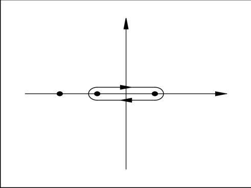
Figure 10: Contour $C$ for calculation of the integral over $x$.

After the substitution $x=\cos\theta_{1}$ the integral over angles is reduced to the integral over contour $C$, presented in Fig. 10:

$$4\pi\int\limits_{-1}^{1}dx\,\frac{x\sqrt{1-x^{2}}}{k^{2}+2klx+l^{2}}=2\pi\oint\limits_{C}dx\,\frac{x\sqrt{1-x^{2}}}{k^{2}+2klx+l^{2}}=$$

$$=4\pi^{2}i\,\mbox{Res}\Bigg{(}\frac{x\sqrt{1-x^{2}}}{k^{2}+2klx+l^{2}},\,x=\infty\Bigg{)}-$$

$$\qquad\qquad\qquad\qquad\qquad\qquad-4\pi^{2}i\,\mbox{Res}\Bigg{(}\frac{x\sqrt{1-x^{2}}}{k^{2}+2klx+l^{2}},\,x=-\frac{k^{2}+l^{2}}{2kl}\Bigg{)}=\qquad$$

$$=4\pi^{2}i\Bigg{(}-\frac{i}{4kl}+\frac{i(k^{2}+l^{2})^{2}}{8k^{3}l^{3}}-\frac{i|k^{2}-l^{2}|(k^{2}+l^{2})}{8k^{3}l^{3}}\Bigg{)}.$$ (111)

Therefore

$$2\pi\oint\limits_{C}dx\,\frac{x\sqrt{1-x^{2}}}{k^{2}+2klx+l^{2}}=\left\{\begin{array}[]{l}{\displaystyle-\frac{\pi^{2}l}{k^{3}},\quad k\geq l;}\\ \\ {\displaystyle-\frac{\pi^{2}k}{l^{3}},\quad l\geq k}\end{array}\right.$$ (115)

and

$$\Lambda\frac{d}{d\Lambda}f_{O}\Big{|}_{p=0}=-\frac{ne^{4}}{8\pi^{2}(2\pi)^{4}}\int\limits_{0}^{\infty}dl\,\frac{l^{2n}/\Lambda^{2n}}{\Big{(}1+l^{2n}/\Lambda^{2n}\Big{)}^{2}}\times$$

$$\qquad\qquad\qquad\quad\ \ \times\Bigg{(}\int\limits_{l}^{\infty}dk\,\frac{l}{k^{3}\Big{(}1+k^{2n}/\Lambda^{2n}\Big{)}}+\int\limits_{0}^{l}dk\,\frac{k}{l^{3}\Big{(}1+k^{2n}/\Lambda^{2n}\Big{)}}\Bigg{)}.\qquad$$ (116)

Making the substitutions $x=l^{2}/\Lambda^{2}$; $y=\Lambda^{2}/k^{2}$ in the first integral and $x=\Lambda^{2}/l^{2}$; $y=k^{2}/\Lambda^{2}$ in the second one, we finally obtain

$$\Lambda\frac{d}{d\Lambda}f_{O}\Big{|}_{p=0}=-\frac{ne^{4}}{32\pi^{2}(2\pi)^{4}}\int\limits_{0}^{\infty}dx\,\frac{x^{n}}{(1+x^{n})^{2}}\int\limits_{0}^{1/x}\frac{dy}{1+y^{-n}}-$$

$$\qquad\qquad\qquad\qquad\qquad\qquad\qquad-\frac{ne^{4}}{32\pi^{2}(2\pi)^{4}}\int\limits_{0}^{\infty}dx\,\frac{x^{n}}{(1+x^{n})^{2}}\int\limits_{0}^{1/x}\frac{dy}{1+y^{n}}=\qquad$$

$$=-\frac{ne^{4}}{32\pi^{2}(2\pi)^{4}}\int\limits_{0}^{\infty}dx\,\frac{x^{n-1}}{(1+x^{n})^{2}}=-\frac{e^{4}}{32\pi^{2}(2\pi)^{4}}=-\frac{\alpha^{2}}{32\pi^{4}}.$$ (117)

Below we also present the identities, which were used for taking integrals, which contain higher derivatives.

1. Identities required for calculation of diagrams with $\phi$- and $\tilde{\phi}$-lines:

$$I_{1}\equiv\int\frac{d^{4}k}{(2\pi)^{4}}\frac{d^{4}l}{(2\pi)^{4}}\frac{d^{4}q}{(2\pi)^{4}}\,\frac{(k+q)^{2}+q^{2}-k^{2}}{k^{2}\Big{(}1+k^{2n}/\Lambda^{2n}\Big{)}\,l^{2}\Big{(}1+l^{2n}/\Lambda^{2n}\Big{)}\,q^{4}(q+k)^{4}(q+l)^{2}}=$$ (119)

$$=\frac{1}{16\pi^{2}}\int\frac{d^{4}k}{(2\pi)^{4}}\frac{d^{4}l}{(2\pi)^{4}}\,\frac{1}{\Big{(}1+k^{2n}/\Lambda^{2n}\Big{)}\,\Big{(}1+l^{2n}/\Lambda^{2n}\Big{)}\,k^{4}l^{4}};$$

$$I_{2}\equiv\int\frac{d^{4}k}{(2\pi)^{4}}\frac{d^{4}l}{(2\pi)^{4}}\,\frac{d^{4}q}{(2\pi)^{4}}\,\frac{1}{k^{2}\Big{(}1+k^{2n}/\Lambda^{2n}\Big{)}\,l^{2}\Big{(}1+l^{2n}/\Lambda^{2n}\Big{)}q^{4}(q+l)^{2}}\times$$

$$\times\Bigg{\{}\frac{12k^{2}}{(q+k)^{2}(q+k+l)^{2}}-\frac{2(k^{4}+k^{2}l^{2})}{(q+k)^{4}(q+k+l)^{2}}-\frac{2k^{2}(k+l)^{2}}{(q+k)^{2}(q+k+l)^{4}}\Bigg{\}}=$$

$$=\frac{1}{4\pi^{2}}\int\frac{d^{4}k}{(2\pi)^{4}}\frac{d^{4}l}{(2\pi)^{4}}\,\frac{1}{\Big{(}1+k^{2n}/\Lambda^{2n}\Big{)}\,\Big{(}1+l^{2n}/\Lambda^{2n}\Big{)}\,k^{4}l^{2}(k+l)^{2}};$$

$$I_{3}\equiv\int\frac{d^{4}k}{(2\pi)^{4}}\frac{d^{4}l}{(2\pi)^{4}}\frac{d^{4}q}{(2\pi)^{4}}\frac{(k+q+l)^{2}+q^{2}-(k+l)^{2}}{k^{2}\Big{(}1+k^{2n}/\Lambda^{2n}\Big{)}\,l^{2}\Big{(}1+l^{2n}/\Lambda^{2n}\Big{)}\,q^{4}(q+k+l)^{4}(q+k)^{2}}=$$

$$=\frac{1}{16\pi^{2}}\int\frac{d^{4}k}{(2\pi)^{4}}\frac{d^{4}l}{(2\pi)^{4}}\,\frac{1}{\Big{(}1+k^{2n}/\Lambda^{2n}\Big{)}\,\Big{(}1+l^{2n}/\Lambda^{2n}\Big{)}}\Bigg{\{}\frac{2}{k^{4}l^{2}(k+l)^{2}}-\frac{1}{k^{4}l^{4}}\Bigg{\}}\quad$$

2. Identities, required for calculation of diagrams with internal Pauli-Villars lines:

$$J_{1}\equiv\int\frac{d^{4}k}{(2\pi)^{4}}\frac{d^{4}l}{(2\pi)^{4}}\frac{d^{4}q}{(2\pi)^{4}}\frac{1}{k^{2}\Big{(}1+k^{2n}/\Lambda^{2n}\Big{)}\,l^{2}\Big{(}1+l^{2n}/\Lambda^{2n}\Big{)}\Big{(}(q+l)^{2}+M^{2}\Big{)}}\times$$

$$\times\Bigg{\{}\frac{1}{(q^{2}+M^{2})^{2}\Big{(}(q+k)^{2}+M^{2}\Big{)}}+\frac{1}{(q^{2}+M^{2})\Big{(}(q+k)^{2}+M^{2}\Big{)}^{2}}-$$

$$-\frac{k^{2}+2M^{2}}{(q^{2}+M^{2})^{2}\Big{(}(q+k)^{2}+M^{2}\Big{)}^{2}}-\frac{2M^{2}}{(q^{2}+M^{2})^{3}\Big{(}(q+k)^{2}+M^{2}\Big{)}}\Bigg{\}}=0;$$ (121)

$$J_{2}\equiv\int\frac{d^{4}k}{(2\pi)^{4}}\frac{d^{4}l}{(2\pi)^{4}}\frac{d^{4}q}{(2\pi)^{4}}\frac{1}{k^{2}\Big{(}1+k^{2n}/\Lambda^{2n}\Big{)}\,l^{2}\Big{(}1+l^{2n}/\Lambda^{2n}\Big{)}(q^{2}+M^{2})^{2}}\times$$

$$\times\frac{1}{\Big{(}(q+k)^{2}+M^{2}\Big{)}\Big{(}(q+l)^{2}+M^{2}\Big{)}}\Bigg{\{}-\frac{k^{2}(k^{2}+l^{2})}{\Big{(}(q+k)^{2}+M^{2}\Big{)}\Big{(}(q+k+l)^{2}+M^{2}\Big{)}}-$$

$$-\frac{2M^{2}(k^{2}+l^{2})}{\Big{(}(q+k)^{2}+M^{2}\Big{)}\Big{(}(q+k+l)^{2}+M^{2}\Big{)}}-\frac{4M^{2}k^{2}}{(q^{2}+M^{2})\Big{(}(q+k+l)^{2}+M^{2}\Big{)}}+$$

$$+\frac{6k^{2}}{\Big{(}(q+k+l)^{2}+M^{2}\Big{)}}-\frac{k^{2}(k+l)^{2}+2M^{2}k^{2}}{\Big{(}(q+k+l)^{2}+M^{2}\Big{)}^{2}}\Bigg{\}}=0;$$ (122)

$$J_{3}\equiv\int\frac{d^{4}k}{(2\pi)^{4}}\frac{d^{4}l}{(2\pi)^{4}}\frac{d^{4}q}{(2\pi)^{4}}\frac{1}{k^{2}\Big{(}1+k^{2n}/\Lambda^{2n}\Big{)}\,l^{2}\Big{(}1+l^{2n}/\Lambda^{2n}\Big{)}(q^{2}+M^{2})^{2}}\times$$

$$\times\frac{1}{\Big{(}(q+k)^{2}+M^{2}\Big{)}\Big{(}(q+k+l)^{2}+M^{2}\Big{)}}\Bigg{\{}3-\frac{(k+l)^{2}+2M^{2}}{\Big{(}(q+k+l)^{2}+M^{2}\Big{)}}-\frac{4M^{2}}{(q^{2}+M^{2})}+$$

$$+\frac{(q+k+l)^{2}+M^{2}}{\Big{(}(q+l)^{2}+M^{2}\Big{)}}-\frac{k^{2}+2M^{2}}{\Big{(}(q+k)^{2}+M^{2}\Big{)}}\Bigg{\}}=0;$$ (123)

$$J_{4}\equiv\int\frac{d^{4}k}{(2\pi)^{4}}\frac{d^{4}l}{(2\pi)^{4}}\frac{d^{4}q}{(2\pi)^{4}}\frac{1}{k^{2}\Big{(}1+k^{2n}/\Lambda^{2n}\Big{)}\,l^{2}\Big{(}1+l^{2n}/\Lambda^{2n}\Big{)}(q^{2}+M^{2})^{2}}\times$$

$$\times\frac{1}{\Big{(}(q+k)^{2}+M^{2}\Big{)}^{2}\Big{(}(q+k+l)^{2}+M^{2}\Big{)}}\Bigg{\{}4M^{2}-\frac{M^{2}(k+l)^{2}+2M^{4}}{\Big{(}(q+k+l)^{2}+M^{2}\Big{)}}+$$

$$+\frac{2M^{2}(q^{2}+M^{2})}{\Big{(}(q+k)^{2}+M^{2}\Big{)}}-\frac{2M^{2}k^{2}+4M^{4}}{\Big{(}(q+k)^{2}+M^{2}\Big{)}}-\frac{4M^{4}}{(q^{2}+M^{2})}\Bigg{\}}=0;$$ (124)

$$J_{5}\equiv\int\frac{d^{4}k}{(2\pi)^{4}}\frac{d^{4}l}{(2\pi)^{4}}\frac{d^{4}q}{(2\pi)^{4}}\frac{1}{k^{2}\Big{(}1+k^{2n}/\Lambda^{2n}\Big{)}\,l^{2}\Big{(}1+l^{2n}/\Lambda^{2n}\Big{)}\Big{(}(q+l)^{2}+M^{2}\Big{)}}\times$$

$$\times\Bigg{\{}\frac{2M^{2}}{\Big{(}q^{2}+M^{2}\Big{)}^{3}\Big{(}(q+k)^{2}+M^{2}\Big{)}}+\frac{M^{2}}{\Big{(}q^{2}+M^{2}\Big{)}^{2}\Big{(}(q+k)^{2}+M^{2}\Big{)}^{2}}-$$

$$-\frac{2M^{4}+M^{2}k^{2}}{\Big{(}q^{2}+M^{2}\Big{)}^{3}\Big{(}(q+k)^{2}+M^{2}\Big{)}^{2}}-\frac{3M^{4}}{\Big{(}q^{2}+M^{2}\Big{)}^{4}\Big{(}(q+k)^{2}+M^{2}\Big{)}}\Bigg{\}}=0;$$ (125)

$$J_{6}\equiv\int\frac{d^{4}k}{(2\pi)^{4}}\frac{d^{4}l}{(2\pi)^{4}}\frac{d^{4}q}{(2\pi)^{4}}\frac{1}{k^{2}\Big{(}1+k^{2n}/\Lambda^{2n}\Big{)}\,l^{2}\Big{(}1+l^{2n}/\Lambda^{2n}\Big{)}(q^{2}+M^{2})^{2}}\times$$

$$\times\frac{1}{\Big{(}(q+k)^{2}+M^{2}\Big{)}\Big{(}(q+l)^{2}+M^{2}\Big{)}}\Bigg{\{}-\frac{2M^{4}}{(q^{2}+M^{2})\Big{(}(q+k+l)^{2}+M^{2}\Big{)}}+$$

$$+\frac{M^{2}\Big{(}(q+l)^{2}+M^{2}\Big{)}-M^{4}}{\Big{(}(q+k+l)^{2}+M^{2}\Big{)}^{2}}-\frac{M^{2}k^{2}}{\Big{(}(q+k+l)^{2}+M^{2}\Big{)}^{2}}+\frac{2M^{2}}{\Big{(}(q+k+l)^{2}+M^{2}\Big{)}}-$$

$$-\frac{M^{2}k^{2}+2M^{4}}{\Big{(}(q+k)^{2}+M^{2}\Big{)}\Big{(}(q+k+l)^{2}+M^{2}\Big{)}}\Bigg{\}}=0.$$ (126)

As an example we prove identity (119). For this purpose we consider

$$I_{1}=\int\frac{d^{4}k}{(2\pi)^{4}}\,\frac{d^{4}l}{(2\pi)^{4}}\,\frac{d^{4}q}{(2\pi)^{4}}\,\frac{2(q^{2}+q_{\mu}k_{\mu})}{k^{2}\Big{(}1+k^{2n}/\Lambda^{2n}\Big{)}\,l^{2}\Big{(}1+l^{2n}/\Lambda^{2n}\Big{)}\,q^{4}(q+k)^{4}(q+l)^{2}}$$ (127)

and write the integral over $d^{4}q$ in four-dimensional spherical coordinates:

$$I_{1}=\int\frac{d^{4}k}{(2\pi)^{4}}\,\frac{d^{4}l}{(2\pi)^{4}}\,\frac{1}{k^{2}\Big{(}1+k^{2n}/\Lambda^{2n}\Big{)}\,l^{2}\Big{(}1+l^{2n}/\Lambda^{2n}\Big{)}}\times$$

$$\qquad\qquad\qquad\times\frac{1}{(2\pi)^{4}}\int d\Omega\,\int\limits_{0}^{\infty}dq\,\frac{2(q+qk\cos\alpha)}{\Big{(}q^{2}+2qk\cos\alpha+k^{2}\Big{)}^{2}\Big{(}q^{2}+2ql\cos\beta+l^{2}\Big{)}}=$$

$$=-\int\frac{d^{4}k}{(2\pi)^{4}}\,\frac{d^{4}l}{(2\pi)^{4}}\,\frac{1}{k^{2}\Big{(}1+k^{2n}/\Lambda^{2n}\Big{)}\,l^{2}\Big{(}1+l^{2n}/\Lambda^{2n}\Big{)}}\times$$

$$\qquad\qquad\quad\ \times\frac{1}{(2\pi)^{4}}\int d\Omega\,\int\limits_{0}^{\infty}dq\,\frac{1}{\Big{(}q^{2}+2ql\cos\beta+l^{2}\Big{)}}\frac{\partial}{\partial q}\frac{1}{\Big{(}q^{2}+2qk\cos\alpha+k^{2}\Big{)}}.\qquad\$$ (128)

Performing integrating by parts in the last integral, we obtain

$$I_{1}=-\int\frac{d^{4}k}{(2\pi)^{4}}\,\frac{d^{4}l}{(2\pi)^{4}}\,\frac{1}{k^{2}\Big{(}1+k^{2n}/\Lambda^{2n}\Big{)}\,l^{2}\Big{(}1+l^{2n}/\Lambda^{2n}\Big{)}}\times$$

$$\qquad\times\frac{1}{(2\pi)^{4}}\int d\Omega\,\Bigg{\{}\frac{1}{\Big{(}q^{2}+2qk\cos\alpha+k^{2}\Big{)}\Big{(}q^{2}+2ql\cos\beta+l^{2}\Big{)}}\Bigg{|}_{0}^{\infty}-$$

$$\qquad\qquad\qquad\qquad-\int\limits_{0}^{\infty}dq\,\frac{1}{\Big{(}q^{2}+2qk\cos\alpha+k^{2}\Big{)}}\frac{\partial}{\partial q}\frac{1}{\Big{(}q^{2}+2ql\cos\beta+l^{2}\Big{)}}\Bigg{\}}=$$

$$=\int\frac{d^{4}k}{(2\pi)^{4}}\,\frac{d^{4}l}{(2\pi)^{4}}\,\frac{1}{k^{2}\Big{(}1+k^{2n}/\Lambda^{2n}\Big{)}\,l^{2}\Big{(}1+l^{2n}/\Lambda^{2n}\Big{)}}\times$$

$$\ \times\frac{1}{(2\pi)^{4}}\int d\Omega\,\Bigg{\{}\frac{1}{k^{2}\,l^{2}}-\int\limits_{0}^{\infty}dq\,\frac{2(q+k\cos\beta)}{\Big{(}q^{2}+2qk\cos\alpha+k^{2}\Big{)}\Big{(}q^{2}+2ql\cos\beta+l^{2}\Big{)}^{2}}\Bigg{\}}=$$

$$=\int\frac{d^{4}k}{(2\pi)^{4}}\,\frac{d^{4}l}{(2\pi)^{4}}\,\frac{1}{k^{2}\Big{(}1+k^{2n}/\Lambda^{2n}\Big{)}\,l^{2}\Big{(}1+l^{2n}/\Lambda^{2n}\Big{)}}\times$$

$$\qquad\qquad\qquad\qquad\qquad\qquad\quad\times\Bigg{\{}\frac{1}{8\pi^{2}}\,\frac{1}{k^{2}\,l^{2}}-\int\frac{d^{4}q}{(2\pi)^{4}}\frac{2(q^{2}+q_{\mu}l_{\mu})}{q^{4}(q+k)^{2}(q+l)^{4}}\Bigg{\}}\qquad$$ (129)

The last integral in this expression is evidently equal to $I_{1}$. Therefore,

$$I_{1}=\frac{1}{16\pi^{2}}\int\frac{d^{4}k}{(2\pi)^{4}}\,\frac{d^{4}l}{(2\pi)^{4}}\,\frac{1}{\Big{(}1+k^{2n}/\Lambda^{2n}\Big{)}\,\Big{(}1+l^{2n}/\Lambda^{2n}\Big{)}\,k^{4}l^{4}}.$$ (130)

The other identities can be derived in the similar way.

Figure 1: One-loop graphs for calculating $\Delta\Gamma_{V}$.

Figure 2: Two-loop graphs for calculating $\Delta\Gamma_{V}$.

Figure 3: Three-loop graphs with two loops of the matter fields. In these diagrams external lines are attached to both loops.

Figure 6: Diagrams, containing an insersion of two-loop counterterms on the matter lines.

Figure 8: Feynman diagrams with two insersions of counterterms.

Figure 9: Two-loop self-energy graphs for matter superfield.