HUTP-03/A027

hep-th/0304080

Greybody factors at large imaginary frequencies
Andrew Neitzke

Jefferson Physical Laboratory, Harvard University,

Cambridge, MA 02138, USA neitzke@fas.harvard.edu

Extending a computation which appeared recently in [1], we compute the transmission and reflection coefficients for massless uncharged scalars and gravitational waves scattered by $d\geq 4$ Schwarzschild or $d=4$ Reissner-Nordstrøm black holes, in the limit of large imaginary frequencies. The transmission coefficient has an interpretation as the “greybody factor” which determines the spectrum of Hawking radiation. The result has an interesting structure and we speculate that it may admit a simple dual description; curiously, for Reissner-Nordstrøm the result suggests that this dual description should involve both the inner and outer horizons. We also discuss some numerical evidence in favor of the formulas of [1].

1 Introduction

Recently there has been a resurgence of interest in certain classical aspects of wave propagation in black hole backgrounds. Specifically, it has been suggested that scattering in the black hole background at large imaginary frequencies may carry information about quantization of the horizon area [2, 3, 4, 5], which has led to some recent investigations of the large-imaginary-frequency behavior. These recent studies [1, 6, 7] mostly focused on the large-imaginary-frequency “quasinormal modes,” which are poles of the transmission coefficient and reflect the black hole’s ringdown response to a perturbation, although [8] also recently studied different aspects of the large-imaginary-frequency behavior using methods similar to those employed in [1] and in this paper.

In Section 2 of this paper we present a computation of the transmission and reflection coefficients for waves traveling from spatial infinity to the black hole horizon, in the limit of large imaginary frequencies: $\omega\to+i\infty$ or more precisely $\lvert\omega r_{H}\rvert\gg 1$, where $r_{H}$ is the horizon radius. We consider here the case of a massless scalar field; then for Schwarzschild black holes in $d\geq 4$, the result is

$$T(\omega) \approx\frac{e^{\beta\omega}-1}{e^{\beta\omega}+3},$$ (1.1)

$$R(\omega) \approx\frac{2i}{e^{\beta\omega}+3},$$ (1.2)

and for Reissner-Nordstrøm in $d=4$ we get

$$T(\omega) \approx\frac{e^{\beta\omega}-1}{e^{\beta\omega}+2+3e^{-\beta_{I}\omega}},$$ (1.3)

$$R(\omega) \approx i\sqrt{3}\frac{1+e^{-\beta_{I}\omega}}{e^{\beta\omega}+2+3e^{-\beta_{I}\omega}}.$$ (1.4)

Here $\beta$ is the inverse Hawking temperature, and for Reissner-Nordstrøm $\beta_{I}$ is the inverse Hawking temperature of the inner horizon; the symbol $\approx$ means that there are ${\mathcal{O}}\left(1/\sqrt{\lvert\omega\rvert r_{H}}\right)$ corrections both to the numerator and to the denominator. The computation is a slight extension of one which recently appeared in [1]; the new result is that we obtain the numerator as well as the denominator. We also calculate $T(\omega)$ and $R(\omega)$ in the limit $\omega\to-i\infty$. The results are summarized in Section 2.3.

As we discuss in Section 2.4, the full result has a suggestive structure; it is strongly reminiscent of the results of [9, 10], which showed that it is possible to reconstruct the effective SCFT description of near extremal black holes by studying $T(\omega)$ for those black holes at small real frequencies. Essentially the idea is that the scattering of Hawking radiation back down the hole by the spacetime curvature modifies the blackbody spectrum in a precise way and makes it agree with the spectrum obtained by an SCFT calculation. We are led to conjecture the existence of an effective description which determines the Hawking radiation at large imaginary frequencies and involves excitations with rather exotic statistics dictated by the denominators of (1.1), (1.3) (such statistics were also proposed in [6] for $d=4$ Schwarzschild). We discuss this conjecture in Section 2.4.

Then switching gears, in Section 3 we discuss the numerical evidence supporting the analytical computations of [1] for the denominators, some of which emerged only very recently [7]. The comparison to the numerical results also clarifies some subtleties about the relation between the formulas for Reissner-Nordstrøm and for Schwarzschild.

We conclude with a few remarks on prospects for future progress. In two appendices, we discuss the analytic structure of the transmission and reflection coefficients and give a few more details of the asymptotic matching procedure used in the computation.

2 The transmission and reflection coefficients

In this section we will compute the transmission and reflection coefficients for waves propagating from infinity to the horizon of a static black hole. The analysis has been carried out so far for Schwarzschild in $d\geq 4$ and for Reissner-Nordstrøm in $d=4$. To be concrete we mostly discuss Schwarzschild in $d=4$; in Section 2.3 we give the results for other cases.

2.1 The wave equation

We consider wave propagation in the exterior region of a Schwarzschild black hole in $d=4$,

$$ds^{2}=-f(r)dt^{2}+f(r)^{-1}dr^{2}+r^{2}d\Omega^{2}.$$ (2.1)

The coordinates (2.1) run from $r_{H}<r<\infty$, where

$$r_{H}=2GM$$ (2.2)

and

$$f(r)=1-r_{H}/r.$$ (2.3)

The propagating field can be a minimally coupled massless scalar, an electromagnetic test-field, or a linearized perturbation of the metric; we label these three possibilities respectively by their spins $j=0,1,2$. In each case the appropriate wave equation is separable. For example, in the $j=0$ case, writing

$$\phi(r,t,\Omega)=r\psi(r)Y_{lm}(\Omega)e^{i\omega t}$$ (2.4)

the massless Klein-Gordon equation $\Delta\phi=0$ becomes a one-dimensional wave equation on the interval $-\infty<x<\infty$, deformed by a potential:

$$\left[-\frac{d^{2}}{dx^{2}}+V[r(x)]-\omega^{2}\right]\psi(x)=0,$$ (2.5)

where

$$V(r)=f(r)\left[\frac{l(l+1)}{r^{2}}+\frac{r_{H}}{r^{3}}\right]$$ (2.6)

and we have introduced the “tortoise coordinate” $x$ defined (up to an additive constant) by

$$x(r)=\int\frac{dr}{f(r)}=r+r_{H}\log(1-r/r_{H}).$$ (2.7)

Wave equations of the form (2.5) also characterize perturbations with $j=1,2$ [11, 12]; only the form of $V(r)$ changes. The three cases can be nicely summarized,

$$V(r)=f(r)\left(\frac{l(l+1)}{r^{2}}+\frac{(1-j^{2})r_{H}}{r^{3}}\right).$$ (2.8)

In our computation it will be convenient to leave $j$ generic and then take the limit $j\to 0$ or $j\to 2$ in the answer. We note that our analysis will depend on the $1/r^{4}$ term in $V(r)$ being dominant; it is therefore singular as $j\to 1$ and we cannot predict the behavior there.

2.2 Transmission and reflection in $d=4$ Schwarzschild

In this section we will compute the transmission and reflection coefficients for (2.5), in the limit of large imaginary frequencies. Most of the ideas required to do this calculation have appeared already in [1], in particular the idea of using the boundary condition at $r_{H}$ to provide the monodromy. The general method of analytic continuation to complex $r$ is much older and has been used successfully for numerical calculations in the past (see [14] for a recent discussion and review.)

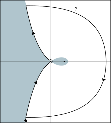
Figure 1: The complex $r$-plane. The $\textrm{Re\ }(x)<0$ region is colored gray, and the points $r=0$, $r=r_{H}$ and a contour $\gamma$ for calculation of the transmission and reflection coefficients are marked. $\gamma$ runs along the line $\textrm{Re\ }(x)=0$ to $\lvert\omega x\rvert\gg 1$ in each direction. The symbol $\bigstar$ represents the direction in which the boundary conditions “at infinity” are imposed.

Although we are studying a wave equation defined on the physical region $r_{H}<r<\infty$, to get the analytic continuation to imaginary $\omega$ we have to consider complex $r$. The behavior of the tortoise coordinate (2.7) at complex $r$ plays an important role in the computation; in particular, since $x(r)$ contains $r_{H}\log(1-r/r_{H})$, it is multivalued, with the branches differing by $\Delta x=2\pi inr_{H}$. This multivaluedness is crucial for our computation. $\textrm{Re\ }x$, however, is uniquely defined; in Figure 1 we have indicated its sign by shading.

The idea of the computation is to study the behavior of a solution $\psi(r)$ to (2.5) as we travel around a specific contour $\gamma$, shown in Figure 1. We will calculate the effect of the trip around $\gamma$ in two different ways: a “local” computation by integrating the differential equation directly and a “global” computation using the boundary conditions at the horizon. Comparing the two gives enough information to calculate the transmission and reflection coefficients.

Since $V(r)$ vanishes faster than $1/\lvert r\rvert$ as $r\to\infty$, as we run to infinity in any direction the asymptotics of a solution to (2.5) are of the form

$$\psi(r)\sim C_{+}e^{+i\omega x}+C_{-}e^{-i\omega x}.$$ (2.9)

In (2.9) there is an ambiguity in defining $e^{\pm i\omega x}$, which arises from the multivaluedness of $x(r)$. This ambiguity implies a compensating ambiguity in defining $C_{\pm}$, even for a fixed $\psi(r)$. This ambiguity is compounded by the fact that $\psi(r)$ itself can have multiple branches, since it is the solution to a differential equation which has singularities. The upshot is that as we travel around $\gamma$ and return to our starting point the coefficients $C_{\pm}$ do not return to their original values (i.e. they have a nontrivial monodromy), because we end up on a different branch both for $x(r)$ and for $\psi(r)$.

As explained in Appendix A, there is a branch cut in $T(\omega)$ and $R(\omega)$ on the positive imaginary $\omega$-axis. If we are on the right side of the branch cut (taking $\textrm{Re\ }\omega$ infinitesimally positive) then $T(\omega)$ and $R(\omega)$ are defined by the boundary conditions

$$\psi\sim\begin{cases}e^{i\omega x}+R(\omega)e^{-i\omega x}&\textrm{\ as\ }r\to\bigstar,\\ T(\omega)e^{i\omega x}&\textrm{\ as\ }r\to r_{H},\end{cases}$$ (2.10)

where $\psi(r)$ is a solution of (2.5). As was done in [1], we will obtain our results by computing in two different ways the monodromy of the coefficient of $e^{-i\omega x}$.

To make this last statement clearer, let us study for a moment the behavior of $\psi(r)$ if we simplify by setting $V(r)=0$. In this case we may replace the asymptotic relation in (2.10) by exact equality: $\psi(r)=e^{i\omega x}+R(\omega)e^{-i\omega x}$ near $\bigstar$. Then we follow $\psi(r)$ along $\gamma$. Since locally we always have free wave propagation in the variable $x$, when we return to $\bigstar$ we still have $\psi(r)=e^{i\omega x}+R(\omega)e^{-i\omega x}$, i.e. the coefficient of $e^{-i\omega x}$ is the same before and after the trip around $\gamma$. On the other hand, $\gamma$ encloses a singularity $r=r_{H}$ around which both $x(r)$ and $\psi(r)$ are multivalued. The boundary condition (2.10) implies that $\psi(r)$ picks up a phase $e^{2\pi\omega r_{H}}$ on any path encircling $r_{H}$ in the clockwise direction. Furthermore, $e^{-i\omega x}$ is multiplied by the phase $e^{-2\pi\omega r_{H}}$ on such a path. These two phases together imply that the coefficient of $e^{-i\omega x}$ must be multiplied by $e^{4\pi\omega r_{H}}$ after the trip around $\gamma$. But we already showed that it is unchanged after this trip; so we get $R(\omega)=e^{4\pi\omega r_{H}}R(\omega)$, which implies $R(\omega)=0$. This is as expected: there is no reflection, since there is no potential! We can calculate $T(\omega)$ by traveling on any contour running from $\bigstar$ to the horizon; then, since we have free wave propagation, the boundary conditions at $\bigstar$ given by (2.10) are propagated directly to the horizon, and comparing with the boundary condition there we see immediately that $T(\omega)=1$. (We also see immediately that $R(\omega)=0$, which we had already concluded above by more elaborate means; the reason for the more complicated discussion above is that it generalizes to the case of a nontrivial potential.)

Now let us consider the real problem at hand, where $V(r)$ is given by (2.8):

$$V(r)=f(r)\left(\frac{l(l+1)}{r^{2}}+\frac{(1-j^{2})r_{H}}{r^{3}}\right).$$ (2.11)

The arguments above still show that $R$ is multiplied by the monodromy $e^{4\pi\omega r_{H}}$ after a trip around $\gamma$; this depended only on the boundary condition (2.10) at $r_{H}$ and the form of $x(r)$. Note that in the black hole context $4\pi r_{H}$ is the inverse Hawking temperature $\beta=1/T_{H}$, so the monodromy can be written $e^{\beta\omega}$.

Now we follow $\gamma$ beginning at $\bigstar$ where we have the boundary condition (2.10). In Appendix A we describe a natural basis $\psi_{\pm}(r)$ of solutions near $r=0$; as discussed there, by asymptotic matching along the line $\textrm{Re\ }x=0$ we can relate the form of $\psi$ slightly southwest of $r=0$ to the form of $\psi$ at $\bigstar$. Namely, if we write the solution southwest of $r=0$ as $\psi(r)=A_{+}\psi_{+}(r)+A_{-}\psi_{-}(r)$, and introduce the notation

$$({\bf{m}})=A_{+}e^{im(1+j)\pi/4}+A_{-}e^{im(1-j)\pi/4},$$ (2.12)

then matching the asymptotics (B.10) of $\psi_{\pm}$ to (2.10) gives

$$({\bf{-1}}) \approx 1,$$ (2.13)

$$({\bf{1}}) \approx R(\omega).$$ (2.14)

Here $\approx$ means there are ${\mathcal{O}}\left(1/\sqrt{\lvert\omega\rvert r_{H}}\right)$ corrections. Next we want to express $T(\omega)$ in terms of $A_{\pm}$. For this we first make a quarter-turn from southwest to southeast, then travel out along $\textrm{Re\ }x=0$ until $\lvert\omega x\rvert\gg 1$, and then run directly to $r=r_{H}$. Since on this trip $\textrm{Re\ }x<0$ and the $\omega^{2}$ term dominates $V(r)$, the WKB (physical optics) approximation guarantees that the coefficient of $e^{i\omega x}$ will not be modified as we travel to the horizon, to leading order in $\omega$. Therefore this coefficient at the horizon is determined simply by the asymptotics of $\psi$ as we run southeast from $r=0$, which are given by (B.8) and (B.10), leading to

$$({\bf{3}})\approx T(\omega).$$ (2.15)

Finally we want to complete our trip around the contour. So we make a three-quarter turn from southwest to northwest, then travel north until $\lvert\omega x\rvert\gg 1$. Then the asymptotic matching using (B.8), (B.10) determines the coefficient of $e^{-i\omega x}$ to be $({\bf{5}})$. On the other hand, we can follow this coefficient around the big semicircle and back to $\bigstar$; again by the WKB approximation it must be unchanged by this trip. But as discussed above, after the full round trip around $\gamma$ the coefficient of $e^{-i\omega x}$ is $e^{\beta\omega}R(\omega)$, so we get

$$({\bf{5}})\approx e^{\beta\omega}R(\omega).$$ (2.16)

The relations (2.13), (2.14), (2.15), (2.16) define an inhomogeneous linear system for the four unknowns $A_{+},A_{-},T(\omega),R(\omega)$. Solving it gives the final answer:

$$T(\omega) \approx\frac{e^{\beta\omega}-1}{e^{\beta\omega}+(1+2\cos\pi j)},$$ (2.17)

$$R(\omega) \approx 2i\frac{\cos\frac{1}{2}\pi j}{e^{\beta\omega}+(1+2\cos\pi j)}.$$ (2.18)

Here the symbol $\approx$ means there can be ${\mathcal{O}}\left(1/\sqrt{\lvert\omega\rvert r_{H}}\right)$ corrections both in the numerator and the denominator. The previous analytical results of [1, 6] for the asymptotic quasinormal frequencies are recovered by looking at the poles of $R(\omega)$ and $T(\omega)$, which occur at $\omega$ satisfying

$$e^{\beta\omega}+(1+2\cos\pi j)\approx 0.$$ (2.19)

In particular, for $j=0$ or $2$ we recover $\textrm{Re\ }\omega\approx T_{H}\log 3$, which was important for [2, 3].

The results (2.17), (2.18) apply for $\omega$ approaching the branch cut from the right, i.e. $\textrm{Re\ }\omega$ infinitesimally positive. If instead we took $\textrm{Re\ }\omega$ infinitesimally negative then the boundary condition at infinity in (2.10) would be set at the north end of Figure 1 rather than at $\bigstar$, and $\gamma$ would run in the opposite direction. The effect is to replace $e^{\beta\omega}$ by $e^{-\beta\omega}$ in (2.16) and hence to replace $\omega$ by $-\omega$ in the final result (still valid for $\omega\to i\infty$.) Then we recover for $j=0$ or $2$ the quasinormal frequencies on the other side of the imaginary axis: $\textrm{Re\ }\omega\approx-T_{H}\log 3$.

We can also study $T(-\omega)$ and $R(-\omega)$ as $\omega\to i\infty$. The analysis is similar to that given above with two differences. First, there are some signs that have to be reversed in the asymptotics (B.10). Taking these signs into account, the analogues of (2.13), (2.14), (2.15) are

$$({\bf{1}}) \approx 1,$$ (2.20)

$$({\bf{-1}}) \approx R(-\omega),$$ (2.21)

$$({\bf{1}}) \approx T(-\omega).$$ (2.22)

Second, the WKB approximation on the large semicircle is now good for the coefficient of $$e^{i\omega x} e^{-i\omega x} e^{2\pi\omega r_{H}}$$ rather than for . For this coefficient the two monodromy factors cancel instead of multiplying, giving instead of (2.16)

$$({\bf{5}}) \approx 1.$$ (2.23)

Solving, we obtain

$$T(-\omega) \approx 1,$$ (2.24)

$$R(-\omega) \approx-2i\cos\frac{1}{2}\pi j.$$ (2.25)

One can also see that $T(-\omega)\approx 1$ directly just by noting that (as discussed in Appendix A) when $\textrm{Im\ }\omega>0$ the analytic continuation is not necessary for defining $T(-\omega)$ and $R(-\omega)$; we can just work directly on the real line, and then the WKB approximation gives $T(-\omega)\approx 1$ immediately since there are no turning points.

2.3 Transmission and reflection for other black holes

The computation of the transmission and reflection coefficients given in Section 2.2 generalizes in a straightforward way to the other black holes considered in [1], with modifications in each case just like the modifications made in [1] for the computation of the quasinormal frequencies. Here we only report the answers. For Schwarzschild in $d\geq 4$ coupled to a massless scalar the result is just as it was in $d=4$: as $\omega\to i\infty$,

$$T(\omega) \approx\frac{e^{\beta\omega}-1}{e^{\beta\omega}+3},$$ (2.26)

$$R(\omega) \approx\frac{2i}{e^{\beta\omega}+3},$$ (2.27)

$$T(-\omega) \approx 1,$$ (2.28)

$$R(-\omega) \approx-2i.$$ (2.29)

For Reissner-Nordstrøm in $$d=4$$ coupled to massless scalar or electromagnetic-gravitational waves the result is

$$T(\omega) \approx\frac{e^{\beta\omega}-1}{e^{\beta\omega}+2+3e^{-\beta_{I}\omega}},$$ (2.30)

$$R(\omega) \approx\pm i\sqrt{3}\frac{1+e^{-\beta_{I}\omega}}{e^{\beta\omega}+2+3e^{-\beta_{I}\omega}},$$ (2.31)

$$T(-\omega) \approx 1,$$ (2.32)

$$R(-\omega) \approx\mp i\sqrt{3},$$ (2.33)

where the sign is determined by the type of field we consider. A useful check on the results is provided by the analytically-continued conservation of flux,

$$T(\omega)T(-\omega)+R(\omega)R(-\omega)=1.$$ (2.34)

2.4 Hawking radiation and greybody factors

Taken together, the results of Section 2.3 for the transmission coefficient at large imaginary frequencies have a rather suggestive structure. To understand it, let us first recall one physical role played by the transmission coefficient at real frequencies.

The spectrum of Hawking radiation seen by a static observer at spatial infinity is not thermal; rather, the particle flux obeys [16]

$$F(\omega)\propto\frac{\lvert T(\omega)\rvert^{2}}{e^{\beta\omega}-1}.$$ (2.35)

The interpretation of this formula is that Hawking radiation is produced with a thermal spectrum at the horizon and then the spacetime curvature between the horizon and infinity scatters some of the radiation back down the hole, so that the thermal spectrum is multiplied by the “greybody factor” $\lvert T(\omega)\rvert^{2}$.

In a remarkable paper [9] it was shown that, for a certain class of near extremal five-dimensional black holes admitting a D-brane construction [17], and for energies small compared to $1/r_{H}$, the greybody factor allows semiclassical general relativity to reproduce the emission spectrum of the appropriate system of D-branes. Namely, for small $\omega$ and in a certain “dilute gas” regime of the black hole parameter space, a direct classical computation gives

$$\lvert T(\omega)\rvert^{2}\approx\frac{e^{\beta\omega}-1}{(e^{\beta_{L}\omega/2}-1)(e^{\beta_{R}\omega/2}-1)},$$ (2.36)

Here $\beta_{L}$ and $\beta_{R}$ are parameters in the classical black hole solution, which can be identified with inverse temperatures characterizing the left-moving and right-moving excitations in an effective SCFT which describes the D-brane degrees of freedom. The factor $e^{\beta\omega}-1$ in (2.36) cancels the denominator of (2.35), leaving the spectrum observed from infinity:

$$F(\omega)\propto\frac{1}{(e^{\beta_{L}\omega/2}-1)(e^{\beta_{R}\omega/2}-1)}.$$ (2.37)

But (2.37) is exactly the emission spectrum calculated from the effective SCFT! To quote [9], “to the observer at infinity the black hole, masquerading in its greybody cloak, looks like the string, for energies small compared to the inverse Schwarzschild radius of the black hole.” Of course, this result was discovered after the D-brane construction was already known; but if the order had been reversed, one might have speculated that this emission spectrum gave a potential clue to the microscopic description of the black hole. This perspective was pursued further in [10] where the calculation of the greybody factor was extended to near extremal charged rotating black holes, both in $d=4$ and $d=5$, and again found to be consistent with an effective SCFT description.

In the present case of the Schwarzschild or Reissner-Nordstrøm black hole we have a similar result, with the important caveat that it does not apply directly to the emission spectrum at real $\omega$. Rather, suppose an observer at spatial infinity measures the exact emission spectrum (for a massless scalar field minimally coupled to the curved background) over some interval of real $\omega$ and then analytically continues to large imaginary $\omega$. What is the result? Using the fact that $T(\omega)^{*}=T(-\omega)$ for real $\omega$, together with (2.26) and (2.28), the analytic continuation of $\lvert T(\omega)\rvert^{2}$ to large imaginary $\omega$ is

$$T(\omega)T(-\omega)\approx\frac{e^{\beta\omega}-1}{e^{\beta\omega}+3}.$$ (2.38)

So substituting in (2.35) we find the same cancellation between the numerator and denominator that occurred in [9]; the observer at infinity would compute a flux which, for large imaginary $\omega$, depends on $\omega$ as

$$F(\omega)\propto\frac{1}{e^{\beta\omega}+3}.$$ (2.39)

Similarly, in the case of the Reissner-Nordstrøm black hole the result is

$$F(\omega)\propto\frac{1}{e^{\beta\omega}+2+3e^{-\beta_{I}\omega}},$$ (2.40)

where $\beta_{I}$ is the inner horizon temperature.

What could these formulas mean? The fact that they are always written in terms of Boltzmann factors (or more properly “Boltzmann phases” since $\omega$ is pure imaginary) is suggestive and we propose that, just as the spectrum of Hawking radiation of a near extremal black hole at small real $\omega$ can be obtained from an effective SCFT, the spectrum of a Schwarzschild or Reissner-Nordstrøm black hole at large imaginary $\omega$ also admits an interpretation in terms of some new degrees of freedom. These degrees of freedom would be expected to have rather exotic statistics (the possibility that the quasinormal modes of $d=4$ Schwarzschild could imply “tripled Pauli statistics” appeared also in [6].) In the Reissner-Nordstrøm case the occurrence of both $e^{\beta\omega}$ and $e^{\beta_{I}\omega}$ suggests further that they should live on both the inner and outer horizons (such descriptions have been considered before, e.g. in [18].) At any rate, the bulk scattering amplitudes we have computed could then be related to correlation functions in this conjectural “boundary” theory. Since our result is valid around large imaginary frequencies it is natural to suspect that this boundary theory bears some relation to the Euclidean continuation of the black hole.

One might wonder why the structure we observe was not already visible in [10]. After all, that paper computed precisely the same function we are computing. The reason our $T(\omega)T(-\omega)$ is not simply the analytic continuation of the $\lvert T(\omega)\rvert^{2}$ in [10] is that both are approximations to the true answer, valid in different regimes. If we know a function $f(\omega)$ exactly at real $\omega$, then we can analytically continue it to get the exact answer for imaginary $\omega$; but if we neglect a small correction at real $\omega$ it can invalidate the continuation to imaginary $\omega$. This problem also occurs when using AdS/CFT to obtain Minkowski space boundary correlators, as discussed recently in [19, 20].

3 Comparison to numerical results

Since some of the asymptotic formulas computed here and in [1, 6] are still new and the result for Reissner-Nordstrøm is rather strange, it may be useful to summarize the numerical evidence supporting them. While I am not aware of any numerical results on the full asymptotic transmission coefficient, there have been several studies of the asymptotic quasinormal frequencies for various types of black hole, to which the analytical results may usefully be compared.

In the case of the Schwarzschild black hole the only numerical results are in $d=4$ and they support the conclusion that the asymptotic real part of the frequency is $T_{H}\log 3$, at least for $j=2$ perturbations [21, 22, 23, 24]. I do not know of any literature on the asymptotic quasinormal frequencies for other $j$. In [22] the corrections at finite $\omega$ were also tabulated; the results there are consistent with the hypothesis that the first subleading correction is ${\mathcal{O}}\left(1/\sqrt{\lvert\omega\rvert r_{H}}\right)$ and proportional to $(l^{2}+l-1)$. This is consistent with an estimate of the correction to the Bessel function asymptotics as discussed in Appendix B, but I have not managed to evaluate the exact coefficient to compare with [22]. Recently [8] appeared containing a computation closely related to the one given here, obtaining the discontinuity across the branch cut of the solution satisfying the outgoing boundary condition at infinity as well as the first correction; this correction was found to be proportional to $(l^{2}+l-1)$ and it is likely that those results can be used to get the correction to the transmission and reflection coefficients as well.

In the case of the Reissner-Nordstrøm black hole in $d=4$, the asymptotic formula for the quasinormal frequencies is more intricate. It is convenient to introduce the parameter

$$\alpha=\frac{1}{1-(r_{I}/r_{H})^{2}},$$ (3.1)

where $r_{I}$ and $r_{H}$ are the inner and outer horizon radii respectively; $\alpha$ runs from $1$ for the uncharged black hole (Schwarzschild limit) to $\infty$ for the extremal black hole. In terms of $\alpha$ and $\hat{\omega}=8\pi GM\omega$, the requirement that the transmission coefficient (1.3) has a pole becomes

$$e^{\alpha\hat{\omega}}+3e^{(\alpha-1)\hat{\omega}}+2\approx 0.$$ (3.2)

The behavior in the asymptotic limit depends crucially on whether $\alpha$ is rational. If $\alpha=p/q$ then we can write $x=e^{\hat{\omega}/q}$ and (3.2) becomes a polynomial equation in $x$, with finitely many solutions. After taking the logarithm each solution then gives an infinite family of quasinormal frequencies, with constant real part and evenly spaced imaginary part; so instead of just one asymptotic real part we have a finite number of them. For example, if $\alpha=2$ we can set $x=e^{\hat{\omega}}$ and then get $x^{2}+3x+2=0$, which has two solutions $x=-1$, $x=-2$, giving two families of asymptotic quasinormal frequencies, at $\hat{\omega}=2\pi i(n+\frac{1}{2})$ and $\hat{\omega}=2\pi i(n+\frac{1}{2})+\log 2$. On the other hand, if $\alpha$ is irrational, the behavior of the asymptotic quasinormal frequencies is more complicated; it probably admits some statistical description in terms of the continued fraction representation of $\alpha$. Such a sensitive dependence on whether $\alpha$ is rational seems strange from the point of view of general relativity, but it might not be so strange from the point of view of an underlying microscopic description of the black hole which makes the parameters discrete.

We can also follow the behavior of a single quasinormal frequency as we increase $\alpha$ from $1$ to $\infty$. At $\alpha=1$ the solutions of (3.2) are simply $\hat{\omega}=2\pi i(n+\frac{1}{2})+\log 5$. Increasing $\alpha$ continuously the frequency traces a spiral in the complex plane, shown in Figure 2 for $n=5$.

Figure 2: Inspiraling behavior of the asymptotic formula (3.2) for the $n=5$ quasinormal frequency as the charge is increased toward extremality. The axes are $\textrm{Re\ }GM\omega$ and $\textrm{Im\ }GM\omega$. The center of the spiral is at $GM\omega=(11/8)i+\log 3/8\pi$.

The center of the spiral corresponds to the extremal limit $\alpha\to\infty$ in which we may neglect the last term of (3.2), obtaining simply $e^{\hat{\omega}}+3\approx 0$, which implies

$$8\pi GM\omega\approx 2\pi i\left(n+\frac{1}{2}\right)+\log 3.$$ (3.3)

Amusingly, this result in the extremal limit agrees with the asymptotic quasinormal frequency for a Schwarzschild black hole of the same mass.

The spiral structure shown in Figure 2 was visible already in the low-order modes computed in [25]. But very recently the full asymptotic formula has been confirmed in detail by the numerical analysis of [7], and looking at their results is useful not only to convince oneself that the formula is asymptotically correct but also to understand the nature of the ${\mathcal{O}}\left(1/\sqrt{\lvert\omega\rvert r_{H}}\right)$ corrections. Rather than looking at the spiral it is convenient to plot $\textrm{Re\ }\omega$ and $\textrm{Im\ }\omega$ separately as functions of the charge $Q$; this is done in Figure 3 for $n=30,5000,10000$.

Figure 3: Real parts (left) and imaginary parts (right) of quasinormal frequencies for the Reissner-Nordstrøm black hole, at mode number (top to bottom) $n=30,5000,10000$. The red line is the numerical data of [7] and the black line is the asymptotic formula (3.2). The vertical axis is (Re or Im) $GM\omega$; the horizontal is $Q$, in units where $Q=1$ is extremal.

We see that at large $n$ the numerical and analytical results agree extremely well, except at small $Q$ where the real part is significantly different even at $n=10000$. How is such a disagreement possible in the asymptotic limit? The point is that, as already mentioned in [1], for the asymptotic formula to be valid one has to take the $n\to\infty$ limit at fixed $Q\neq 0$. In this limit we will eventually find agreement with the asymptotic formula (e.g. if we fix $Q=0.16$, we can see from Figure 3 that $n=5000$ is not sufficiently large for the asymptotic behavior to take over, but $n=10000$ is.) The required $n$ diverges as $Q\to 0$, or put another way, the ${\mathcal{O}}\left(1/\sqrt{\lvert\omega\rvert r_{H}}\right)$ corrections to the asymptotic formula (3.2) appear with a coefficient which diverges as $Q\to 0$. A more systematic analysis of these corrections should demonstrate this behavior explicitly; here we only remark that the analysis in [1] which led to (3.2) is certainly singular in the limit $Q\to 0$, so we would expect that the corrections would indeed blow up.

4 Conclusions

In this paper we have presented some results about the scattering of free massless quantum fields by a black hole, in the limit of large imaginary frequencies. These results stand independent of any speculation about their meaning, but their form is tantalizing and it seems that they deserve to have a simple explanation. The remarks about a possible boundary interpretation which appear in Section 2.4 are of course pure conjecture at the moment; hopefully the situation will be clarified in the future.

It remains unclear whether one can connect the computation presented here to the area-quantization ideas which motivated the consideration of the high-imaginary-frequency quasinormal modes in [2, 3]. It is clear that these ideas will have to be modified or reinterpreted in some way if they are to be correct, since the Reissner-Nordstrøm and Kerr black holes do not share the simple behavior seen in the Schwarzschild case. Nevertheless, it is possible that this could be done, and the spin-network picture discussed in [3] could be a candidate for the boundary description we are conjecturing.

There are several other calculations along the same lines which could be done and might shed some light on the situation. One possibility would be to include chemical potentials, either by studying a rotating black hole or a charged scalar in the Reissner-Nordstrøm background. In both cases one faces the technical difficulty that the potentials appear to be long-range (they involve $1/r$) and hence the behavior is not simply plane-wave at infinity. In the rotating case, at least for the Kerr black hole, this problem can be avoided by a clever change of variable introduced by Sasaki and Nakamura [26], but the problem remains difficult because the angular equation also has to be treated approximately (the centrifugal potential, which was just $l(l+1)/r^{2}$ for Schwarzschild and had no effect to leading order in $\omega$, depends on $\omega$ for Kerr.) For Reissner-Nordstrøm I am not aware of a change of variables which makes the potential short-range, but it should be possible to make one and this problem might be more tractable than Kerr. On the other hand, in the Kerr case there are some numerical results available [7] which look puzzling but might be helpful. One could also study the high-imaginary-frequency behavior for fermionic fields. Here the relevant radial equation has been given e.g. in [27], and the low overtone quasinormal modes were recently considered in [28].

Another possibility would be to apply our method to the five-dimensional near extremal black holes studied in [9, 17], for which we already have not only an effective SCFT but a full microscopic description, and see whether the resulting large-imaginary-frequency behavior can fit into that description somewhere.

Appendix A Generalities on one-dimensional wave equations

The notions of transmission and reflection coefficient for a one-dimensional wave equation are well known, at least for real frequencies. However, there are some subtleties associated with analytic continuation to complex frequencies. Under fairly general conditions this analytic continuation does exist; the questions are what its singularities are and whether we can construct it in a way which facilitates explicit computation.

Suppose given a wave equation on the real line $-\infty<x<\infty$ with the form of (2.5),

$$\left[-\frac{d^{2}}{dx^{2}}+V(x)-\omega^{2}\right]\psi(x)=0,$$ (A.1)

where $V(x)\to 0$ faster than $1/\lvert x\rvert$ as $x\to\pm\infty$. We can then define $T(\omega),R(\omega)$ for waves of real frequency $\omega\neq 0$ by fixing the boundary conditions

$$\psi(x)\sim\begin{cases}T(\omega)e^{+i\omega x}&\textrm{\ as\ }x\to-\infty,\\ e^{+i\omega x}+R(\omega)e^{-i\omega x}&\textrm{\ as\ }x\to+\infty.\end{cases}$$ (A.2)

The boundary conditions (A.2) also suffice to extend $T(\omega)$ and $R(\omega)$ to complex-analytic functions on the lower half-plane $\textrm{Im\ }\omega<0$. Furthermore these functions are nonsingular; there cannot be any poles because they would imply the existence of a normalizable solution to (A.1) with complex $\omega$, which is impossible because of the self-adjointness of $-d^{2}/dx^{2}+V(x)$.

It is not straightforward to define $T(\omega)$ or $R(\omega)$ for $\omega$ in the upper half-plane, because in that case the boundary condition (A.2) as $x\to+\infty$ does not give a constraint on the solution; the solution $e^{+i\omega x}$ is exponentially small compared to $e^{-i\omega x}$ as $x\to+\infty$, so adding $e^{+i\omega x}$ with an arbitrary coefficient does not affect the asymptotics as $x\to+\infty$, and there is no way to define what we mean by requiring this coefficient to be $1$. In some cases we can nevertheless analytically continue $T(\omega)$ to the upper half-plane; the existence and singularity structure of such a continuation depend on the properties of $V(x)$. We now turn to some examples.

The simplest possibility is $V(x)=0$ for all $x$. In this case the prescription above gives simply $T(\omega)=1,R(\omega)=0$ for all $\omega$ in the lower half-plane, which has the obvious analytic continuation $T(\omega)=1,R(\omega)=0$ for all $\omega$.

Another possibility is that $V(x)\neq 0$ but $V(x)$ strictly vanishes as $x\to\pm\infty$ (e.g. a finite square well). In that case, for any $\omega$, the solutions of (A.1) near $\pm\infty$ are strict linear combinations of $e^{\pm i\omega x}$. Therefore $T(\omega)$ can be uniquely defined for any $\omega$ just by replacing the asymptotic relation $\sim$ by exact equality in (A.2). This prescription defines $T(\omega)$ and $R(\omega)$ univalently for any $\omega\neq 0$, so $T(\omega)$ and $R(\omega)$ are single-valued, although they can have isolated singularities at $\omega=0$ and in the upper half-plane.

A third possibility is that $V(x)$ admits analytic continuation to complex $x$ and furthermore $V(x)\to 0$ faster than $1/\lvert x\rvert$ as $x\to\infty$ in any direction (e.g. $V(x)=1/(x^{2}+1)$.) Note that this case and the one just considered are mutually exclusive. In this case we can define $T(\omega)$ by setting our boundary conditions on the line $\omega x\in{\mathbb{R}}$ rather than $x\in{\mathbb{R}}$:

$$\psi(x)\sim\begin{cases}T(\omega)e^{+i\omega x}&\textrm{\ as\ }\omega x\to-\infty,\\ e^{+i\omega x}+R(\omega)e^{-i\omega x}&\textrm{\ as\ }\omega x\to+\infty.\end{cases}$$ (A.3)

The advantage of (A.3) over (A.2) is that the solutions are oscillatory on the line $\omega x\in{\mathbb{R}}$ and hence the asymptotics (A.3) determine $T(\omega)$ and $R(\omega)$. There is one additional complication: if $V(x)$ has singularities along the line $\omega x\in{\mathbb{R}}$, then $\psi(x)$ will generally be multivalued, so we have to specify the contour along which we travel from one side of the line $\omega x\in{\mathbb{R}}$ to the other. To make $T(\omega)$ and $R(\omega)$ holomorphic in $\omega$ the only option is to continuously deform the contour by “Wick rotation” from the real axis; but then after a full $2\pi$ rotation the contour will hang on the singularities, so $T(\omega)$ and $R(\omega)$ are potentially multivalued.

Finally we come to the case which actually occurs for black hole transmission coefficients, say for $d=4$ Schwarzschild. Here the analytic structure of $T(\omega)$ and $R(\omega)$ has been extensively studied because it is relevant for the long time behavior of black hole perturbations; see in particular [29]. In this case $V(x)=V[r(x)]$, with $r(x)$ defined implicitly by (2.7), and while $V(r)$ is manifestly single-valued all over the complex $r$-plane, $r(x)$ generally has multiple branches (because of the logarithm in (2.7)). So the analytic continuation of $V(x)$ is a multivalued function of $x$. Nevertheless, since the only singularity of $V(r)$ occurs at $r=0$, the singularities of $V[r(x)]$ can only occur at $x$ for which some branch of $r(x)$ has $r(x)=0$, namely at $x=2\pi in$. So $T(\omega)$, $R(\omega)$ can be defined by Wick rotation of the $x$-plane contour to any $\omega$ with $\textrm{Re\ }\omega\neq 0$. However, at $\textrm{Re\ }\omega=0$ we encounter an infinite chain of singularities and we have to choose which way to go around them; our choice will depend on which way we made the Wick rotation (i.e. whether we are coming from $\textrm{Re\ }\omega>0$ or $\textrm{Re\ }\omega<0$). $T(\omega),R(\omega)$ therefore have branch cuts at positive imaginary $\omega$. In the body of the paper we compute these functions for $\omega$ on the right side of the cut, i.e. $\textrm{Re\ }\omega$ infinitesimally positive; in that case, after performing the Wick rotation in the $x$-plane, (A.3) corresponds to (see Figure 1 in Section 2.2)

$$\psi(r)\sim\begin{cases}T(\omega)e^{+i\omega x}&\textrm{\ as\ }r\to r_{H},\\ e^{i\omega x}+R(\omega)e^{-i\omega x}&\textrm{\ as\ }r\to\bigstar.\end{cases}$$ (A.4)

If we had assumed $\textrm{Re\ }\omega<0$ instead, we would have put $\bigstar$ at the north of Figure 1 instead of the south.

Appendix B Asymptotics of solutions to the wave equation

In our analysis of the solutions of (2.5) along the line $\textrm{Re\ }x=0$ we need to know their asymptotics in the limit $\omega\to i\infty$. In this limit the term $\omega^{2}$ dominates the potential everywhere except near $r=0$, so we expect that the interesting behavior will occur there. Near $r=0$ we have from (2.7)

$$x/r_{H}=r/r_{H}+\log(1-r/r_{H})=-\frac{1}{2}(r/r_{H})^{2}-\frac{1}{3}(r/r_{H})^{3}+{\mathcal{O}}\left((r/r_{H})^{4}\right)$$ (B.1)

which can be inverted to obtain

$$r/r_{H}=\pm i\sqrt{2x/r_{H}}+2x/3r_{H}+{\mathcal{O}}\left((x/r_{H})^{3/2}\right)$$ (B.2)

Substituting this in (2.5), (2.8) we obtain the leading-order behavior of (2.5) near the $r=0$ singularity together with its first correction:

$$\left[-\frac{d^{2}}{dx^{2}}+\frac{j^{2}-1}{4x^{2}}\pm i\frac{\eta}{x^{3/2}\sqrt{r_{H}}}+{\mathcal{O}}\left((xr_{H})^{-1}\right)-\omega^{2})\right]\psi=0,$$ (B.3)

with

$$\eta=\frac{(j^{2}-1)-3l(l+1)}{6\sqrt{2}}.$$ (B.4)

Further setting $\rho=\omega x$,

$$\left[-\frac{d^{2}}{d\rho^{2}}+\frac{j^{2}-1}{4\rho^{2}}\pm i\frac{\eta}{\rho^{3/2}\sqrt{\omega r_{H}}}+{\mathcal{O}}\left(\frac{1}{\rho\omega r_{H}}\right)-1\right]\psi=0$$ (B.5)

Integrating the subleading terms twice in $\rho$ shows they can at worst give corrections where $\delta\psi/\psi$ scales as a power of $\rho/\omega r_{H}$. Then in the $\omega\to i\infty$ limit with $\rho\ll 1$, one may neglect this term as well as the constant term $1$ and write simply

$$\left[\frac{d^{2}}{d\rho^{2}}+\frac{1-j^{2}}{4\rho^{2}}\right]\psi=0.$$ (B.6)

So when $\rho\ll 1$ there are two possibilities for the asymptotics:

$$\psi(\rho)\sim\rho^{(1\pm j)/2}.$$ (B.7)

It turns out that both possibilities occur and we can pick two linearly independent solutions $\psi_{\pm}$ by fixing their rotation properties (at least for non-integer $j$):

$$\psi_{\pm}(e^{i\theta}\rho)=e^{(1\pm j)i\theta/2}\psi_{\pm}(\rho).$$ (B.8)

On the other hand, for $1\ll\rho$, (B.5) is simply

$$\left[\frac{d^{2}}{d\rho^{2}}+1\right]\psi=0$$ (B.9)

and so the solutions are asymptotic to free waves $e^{\pm i\rho}$. The issue is now to interpolate between these two regions. To leading order in $\omega$ this can be done by neglecting the $1/\sqrt{\omega}$ term in (B.5); one then finds that $\psi_{\pm}$ are asymptotic to $\sqrt{\rho}J_{\pm j/2}(\rho)$ in the region $\rho\ll\lvert\omega\rvert r_{H}$, and since this region overlaps with the region $1\ll\rho$ in the limit of large $\omega$, one can match the known asymptotics of Bessel functions to the free wave propagation. This was the approach taken in [1] and it gives for $1\ll\rho$

$$\psi_{\pm}(\rho)\sim\cos(\rho-(1\pm j)\pi/4)+{\mathcal{O}}\left(1/\sqrt{\lvert\omega\rvert r_{H}}\right).$$ (B.10)

From (B.4), (B.5) we see that the ${\mathcal{O}}\left(1/\sqrt{\lvert\omega\rvert r_{H}}\right)$ correction to (B.10) should be proportional to $(j^{2}-1)-3l(l+1)$; in the case $j=2$ this dependence was also found in [8], where in addition the exact numerical coefficient was evaluated.

References

- [1] L. Motl and A. Neitzke, “Asymptotic black hole quasinormal frequencies,” hep-th/0301173.
- [2] S. Hod, “Bohr’s correspondence principle and the area spectrum of quantum black holes,” Phys. Rev. Lett. 81 (1998) 4293, gr-qc/9812002.
- [3] O. Dreyer, “Quasinormal modes, the area spectrum, and black hole entropy,” Phys. Rev. Lett. 90 (2003) 081301, gr-qc/0211076.
- [4] A. Corichi, “On quasinormal modes, black hole entropy, and quantum geometry,” gr-qc/0212126.
- [5] S. Hod, “Kerr black hole quasinormal frequencies,” gr-qc/0301122.
- [6] L. Motl, “An analytical computation of asymptotic Schwarzschild quasinormal frequencies,” gr-qc/0212096.
- [7] E. Berti and K. D. Kokkotas, “Asymptotic quasinormal modes of Reissner-Nordstroem and Kerr black holes,” hep-th/0303029.
- [8] A. Maassen van den Brink, “WKB analysis of the Regge–Wheeler equation down in the frequency plane,” gr-qc/0303095.
- [9] J. M. Maldacena and A. Strominger, “Black hole greybody factors and D-brane spectroscopy,” Phys. Rev. D55 (1997) 861–870, hep-th/9609026.
- [10] J. M. Maldacena and A. Strominger, “Universal low-energy dynamics for rotating black holes,” Phys. Rev. D56 (1997) 4975–4983, hep-th/9702015.
- [11] J. Wheeler, “Geons,” Phys. Rev. 97 (1955) 511.
- [12] T. Regge and J. A. Wheeler, “Stability of a Schwarzschild singularity,” Phys. Rev. 108 (1957) 1063.
- [13] S. Chandrasekhar, The mathematical theory of black holes. Oxford University Press, Oxford, UK, 1985. International series of monographs on physics, 69.
- [14] K. Glampedakis and N. Andersson, “Quick and dirty methods for studying black-hole resonances,” gr-qc/0304030.
- [15] E. C. Kemble Phys. Rev. 48 (1935) 549.
- [16] S. W. Hawking, “Particle creation by black holes,” Commun. Math. Phys. 43 (1975) 199–220.
- [17] A. Strominger and C. Vafa, “Microscopic origin of the Bekenstein-Hawking entropy,” Phys. Lett. B379 (1996) 99–104, hep-th/9601029.
- [18] C. Vaz and L. Witten, “The quantum states and the statistical entropy of the charged black hole,” Phys. Rev. D63 (2001) 024008, gr-qc/0006039.
- [19] D. T. Son and A. O. Starinets, “Minkowski-space correlators in AdS/CFT correspondence: Recipe and applications,” JHEP 09 (2002) 042, hep-th/0205051.
- [20] C. P. Herzog and D. T. Son, “Schwinger-Keldysh propagators from AdS/CFT correspondence,” hep-th/0212072.
- [21] E. W. Leaver, “An analytic representation for the quasi-normal modes of Kerr black holes,” Proc. R. Soc. Lond. A402 (1985) 285–298.
- [22] H.-P. Nollert, “Quasinormal modes of Schwarzschild black holes: The determination of quasinormal frequencies with very large imaginary parts,” Phys. Rev. D47 (1993) 5253–5258.
- [23] N. Andersson, “On the asymptotic distribution of quasinormal-mode frequencies for Schwarzschild black holes,” Class. Quantum Grav. 10 (1993) L61–L67.
- [24] A. Bachelot and A. Motet-Bachelot, “The resonances of a Schwarzschild black hole (French),” Annales Poincare Phys. Theor. 59 (1993) 3.
- [25] N. Andersson and H. Onozawa, “Quasinormal modes of nearly extreme Reissner-Nordstroem black holes,” Phys. Rev. D54 (1996) 7470–7475, gr-qc/9607054.
- [26] M. Sasaki and T. Nakamura, “A class of new perturbation equations for the Kerr geometry,” Phys. Lett. A89 (1982) 68–70.
- [27] B. Mukhopadhyay and S. K. Chakrabarti, “Semianalytical solution of Dirac equation in Schwarzschild geometry,” Class. Quant. Grav. 16 (1999) 3165–3181, gr-qc/9907100.
- [28] H. T. Cho, “Dirac quasi-normal modes in Schwarzschild black hole spacetimes,” gr-qc/0303078.
- [29] E. W. Leaver, “Spectral decomposition of the perturbation response of the Schwarzschild geometry,” Phys. Rev. D 34 (1986) 384–408.