Pair creation by homogeneous electric field from the point of view of an accelerated observer

Abstract

With a special choice of gauge the operator of the Klein-Fock-Gordon equation in homogeneous electric field respects boost symmetry. Using this symmetry we obtain solutions for the scalar massive field equation in such a background (boost modes in the electric field). We calculate the spectrum of particles created by the electric field, as seen by an accelerated observer at spatial infinity of the right wedge of Minkowski spacetime. It is shown that the spectrum and the total number of created pairs measured by a remote uniformly accelerated observer in Minkowski spacetime are precisely the same as for inertial observers.

, , ,

1. The Schwinger process of pair creation by a constant electric field from vacuum [1] have been studied in details (using different methods and different gauges of the external field) in the early 70-s [2, 3, 4, 5, 6, 7]. In this literature the quantum states of created particles were labelled either by values of generalized momentum (non-stationary gauge) or energy (stationary gauge). However the constant electric field permits another symmetry which is based on invariance of the field with respect to Lorentz transformations along its direction. If the field is directed along the $z$-axis, this symmetry is generated by the boost operator $\mathcal{B}=i(t\partial/{\partial z}+z\partial/{\partial t})$. The presence of boost symmetry in the problem makes it very similar to the problem of particle creation by an eternal black hole [8, 9]. Thus treatment of the Schwinger process in terms of boost modes is of great importance for the quantum field theory in curved spacetime.

Besides providing a possible algorithm for investigation of the process of particle creation in the background of eternal black hole, the boost modes based approach to the Schwinger problem is of independent interest. It is very natural to use Milne–Rindler coordinate map (see, e.g., [9]) in problems with boost symmetry. Physically transition to these coordinates means transition to a non-inertial reference frame, namely, to a uniformly accelerated reference frame in the right and left wedges of Minkowski spacetime (MS). We know the average number of particles created by a constant electric field as it is seen in inertial reference frames. Therefore calculation of this quantity measured by an accelerated observer will clear up the question of how inertial forces influence the spectrum and the total number of created particles.

2. We consider the Schwinger problem for massive scalar particles where for the electric field $E$ we chose a special gauge

$$A_{\mu}=-(E/2)\epsilon_{\mu\nu}x^{\nu},\quad x^{\mu}=\{t,z\},\,\;\epsilon_{\mu\nu}=-\epsilon_{\nu\mu},\;\epsilon_{tz}=1,$$ (1)

which provides invariance of the Klein-Fock-Gordon (KFG) equation under boost transformations. The latter equation in the gauge (1) takes the form

$$\left(\square-eE\mathcal{B}+\frac{1}{4}e^{2}E^{2}x_{+}x_{-}+m^{2}\right)\phi(x)=0,$$ (2)

where $e$ and $m$ are the electric charge and mass of the particle, $x_{\pm}=t\pm z,\;\square=4\partial^{2}/\partial x_{+}\partial x_{-}$ and the boost generator $\mathcal{B}=\mathcal{D}_{(+)}-\mathcal{D}_{(-)},\;\mathcal{D}_{(\pm)}=ix_{\pm}\partial/\partial x_{\pm}.$ One can easily check that the KFG operator at the l.h.s. of Eq.(2) commutes with $\mathcal{B}$. Therefore solutions for equation (2) can be labelled by eigenvalues $\kappa$ of the boost generator $\mathcal{B}$. We will call the solutions to Eq.(2) $\phi_{\kappa}(x)$ satisfying the equation $\mathcal{B}\phi_{\kappa}=\kappa\phi_{\kappa}$ ”the boost modes in the electric field”.

The commuting boost $\mathcal{B}$ and dilatation $\mathcal{D}=\mathcal{D}_{(+)}+\mathcal{D}_{(-)}$ vector fields generate local pseudoeuclidean coordinates which admit separation of variables in Eq. (2). In the future ($F$) and past ($P$) wedges of MS, see Fig.1, these are Milne coordinates

$$\tau=\pm m(x_{+}x_{-})^{1/2},\;\sigma=1/2\ln(x_{+}/x_{-}),$$ (3)

while in the Rindler right ($R$) and left ($L$) wedges, Rindler coordinates

$$\eta=1/2\ln(-x_{+}/x_{-}),\;\rho=\pm m(-x_{+}x_{-})^{1/2},$$ (4)

(compare to [9]). The four regions $R$, $L$, $P$ and $F$ are bounded by horizons which belong to the light cone $x^{2}\equiv t^{2}-z^{2}=0$, and (together with the horizons and the origin $x=0$) cover the whole MS. Since the coordinate lines $\rho=const$ in the Rindler wedges $R$ and $L$ coincide with the world lines of uniformly accelerated observers in MS the resulting reference frame can be considered as a uniformly accelerated one.

3. It was shown in Refs. [3, 10] that classical solutions for the relevant field equation contain complete information on the pair creation process. Here we will follow these papers in our analysis instead of constructing a consistent second quantized theory. We will assume that the initial state of the field in $P$-wedge at far past ($\tau\rightarrow-\infty,$ or $x_{\pm}\rightarrow-\infty$) is a vacuum state.

It follows from [3, 10] that there exist two non-equivalent complete sets of modes in the Schwinger problem. It was shown in [10] that complete information on the pair creation process can be derived from any solution belonging to any of the sets. It is convenient for us to use the solution which in the $P$-wedge takes the form

$$\begin{array}[]{c}\displaystyle\phi_{\kappa}(x)=\frac{1}{\sqrt{2}}(-mx_{-})^{i\kappa}\exp\left\{-\frac{i}{4}\,\mathcal{E}m^{2}x_{+}x_{-}-\frac{\pi}{4\,\mathcal{E}}\right\}\times\\ \\ \displaystyle\times\Psi\left(\frac{1}{2}+\frac{i}{2\,\mathcal{E}}\,,\,1+i\kappa\,,\frac{i}{2}\,\mathcal{E}m^{2}x_{+}x_{-}\right),\end{array}$$ (5)

where $\mathcal{E}=E/E_{cr}$ is the electric field strength in the units of critical QED field $E_{cr}=m^{2}c^{3}/e\hbar$, and $\Psi(a,c,\zeta)$ is the Tricomi function [11]. The explicit form for the solution (5) in other wedges may be obtained by analytic continuation in such a way that for transitions from one wedge to another one should use substitutions $-x_{\pm}\rightarrow x_{\pm}e^{-i\pi},$ (compare to Ref. [12]). At the limit $E\rightarrow 0$ the modes (5) coincide up to a phase factor with the boost modes $\;\Psi^{*}_{-\kappa}(x)$ for empty MS, see Ref. [12].

Let us first analyze the particle creation process in the $P$-wedge. Using the asymptotic expression for the Tricomi function [11] we can see that at far past ($x_{\pm}\to-\infty$) the solution (5) acquires semiclassical form

$$\phi_{\kappa}(x)=(2\,|\mathcal{D}S_{\kappa}|)^{-1/2}\exp(iS_{\kappa}),$$ (6)

where

$$S_{\kappa}(x_{+},x_{-})=-\frac{\mathcal{E}}{4}\,m^{2}x_{+}x_{-}-\frac{1}{2\,\mathcal{E}}\ln\left(m^{2}x_{+}x_{-}\right)+\kappa\ln(-mx_{-})+\ldots$$

is the classical action of a particle with a charge $e$ moving in the electric field (1). This solution is normalized by the condition $\mathcal{J}^{\,\tau}=-e$ which means that the charge per unit interval of $\sigma$ in the local reference frame is equal to $-e$. Hence, in the in-region the solution (5) describes an incoming antiparticle accelerated by the electric field $E$. Here

$$\mathcal{J}^{\mu}=e\sqrt{-g}g^{\mu\nu}\left(i\phi_{\kappa}^{*}\frac{{{\displaystyle\leftrightarrow}\atop{\displaystyle\partial}}}{\partial x^{\nu}}\varphi_{\kappa}-2eA_{\nu}\phi_{\kappa}^{*}\phi_{\kappa}\right),$$

is the vector density of current, $\tau$-component of which for the wedge $P$ can be represented in the form $\;\mathcal{J}^{\,\tau}=-e\phi_{\kappa}^{*}\!\!\stackrel{{\scriptstyle\displaystyle\leftrightarrow}}{{\displaystyle\mathcal{D}}}\!\!\phi_{\kappa}$.

Near the light cone $x_{+}x_{-}=0$ the solution (5) reduces to [11]

$$\begin{array}[]{r}\displaystyle\phi_{\kappa}(x)\sim\frac{1}{\sqrt{2}}e^{-\pi/4\,\mathcal{E}}\frac{\Gamma(-i\kappa)}{\Gamma(1/2+i/2\,\mathcal{E}-i\kappa)}(-mx_{-})^{i\kappa}+\\ \\ \displaystyle+\frac{1}{\sqrt{2}}e^{\pi\kappa/2-\pi/4\,\mathcal{E}}\frac{\Gamma(i\kappa)}{\Gamma(1/2+i/2\,\mathcal{E})}\left(-\frac{\mathcal{E}}{2}mx_{+}\right)^{-i\kappa}.\end{array}$$ (7)

The first term at the r.h.s. is obviously a wave propagating to the right, while the second term is a wave propagating to the left, both waves travelling with the speed of light. Near the horizon the charge densities carried by the right- and left-going waves are respectively given by

$$\begin{array}[]{cc}\displaystyle\mathcal{J}^{\,\tau}_{(-)}=-ie\phi_{\kappa}^{*}\stackrel{{\scriptstyle\displaystyle\leftrightarrow}}{{\displaystyle D}}_{(-)}\phi_{\kappa}=\,e\frac{1+e^{2\pi\kappa-\pi/\mathcal{E}}}{e^{2\pi\kappa}-1},\\ \\ \displaystyle\mathcal{J}^{\,\tau}_{(+)}=-ie\phi_{\kappa}^{*}\stackrel{{\scriptstyle\displaystyle\leftrightarrow}}{{\displaystyle D}}_{(+)}\phi_{\kappa}=-e\frac{1+e^{-\pi/\mathcal{E}}}{1-e^{-2\pi\kappa}}.\end{array}$$ (8)

It is easily seen that $\mathcal{J}^{\,\tau}_{(-)}>0$ and $\mathcal{J}^{\,\tau}_{(+)}<0$ if $\kappa>0$. This means that the right-going wave describes the flux of particles created by the electric field, while the left-going wave describes the flux of created antiparticles together with the incoming one. Thus, these charge densities should be written in the form, compare [3, 10] $\mathcal{J}^{\,\tau}_{(-)}=en_{\kappa}^{(P)}$, $\mathcal{J}^{\,\tau}_{(+)}=-e\left(1+n_{\kappa}^{(P)}\right)$, where $n_{\kappa}^{(P)}$ is the number of pairs in the $\kappa$-th mode, created by the electric field from vacuum in the $P$-wedge. Obviously, we have:

$$n_{\kappa}^{(P)}=\frac{1+e^{2\pi\kappa-\pi/\mathcal{E}}}{e^{2\pi\kappa}-1},\quad\kappa>0.$$ (9)

If $\kappa<0$, $\mathcal{J}^{\,\tau}_{(-)}<0$ and $\mathcal{J}^{\,\tau}_{(+)}>0$. Therefore in this case the right-going wave describes the flux of antiparticles, while the left-going wave describes the flux of particles, and the corresponding charge densities should be written in the form $\mathcal{J}^{\,\tau}_{(-)}=-e\left(1+n_{\kappa}^{(P)}\right)$,  $\mathcal{J}^{\,\tau}_{(+)}=en_{\kappa}^{(P)}$ with

$$n_{\kappa}^{(P)}=\frac{1+e^{-\pi/\mathcal{E}}}{e^{2\pi|\kappa|}-1},\quad\kappa<0.$$ (10)

Thus we conclude that for $\kappa>0$ particles created in the $P$-wedge travel to the $R$-wedge and the antiparticles to the $L$-wedge, while for negative values of $\kappa$ we have the opposite situation.

4. Now let us consider what happens in the $R$-wedge. In terms of Rindler coordinates (4) the KFG equation (2) after separation of the time-like variable $\eta,\;\phi_{\kappa}=e^{-i\kappa\eta}\varphi_{\kappa}(\rho),$ formally coincides with the stationary Schrödinger equation with respect to the independent variable $u=\ln{\rho}$

$$\left[-\frac{d^{2}}{du^{2}}+U_{\kappa}\right]\varphi_{\kappa}=\kappa^{2}\varphi_{\kappa},$$ (11)

where the effective potential reads

$$U_{\kappa}(\rho)=(1-\mathcal{E}\kappa)\rho^{2}-\frac{1}{4}\,\mathcal{E}^{2}\rho^{4},\quad\rho=e^{u}.$$ (12)

If $\kappa\geq 1/\mathcal{E}$, the effective potential is monotonously decreasing with $\rho^{2}$. If $\kappa<1/\mathcal{E}$, then $U_{\kappa}(\rho)$ is a potential of barrier type with maximum $U_{\kappa}^{(m)}$ at $\rho=\rho_{m}$

$$\rho_{m}^{2}=2\mathcal{E}^{-1}(\mathcal{E}^{-1}-\kappa),\quad U_{\kappa}^{(m)}=(\mathcal{E}^{-1}-\kappa)^{2}.$$ (13)

However real solutions for the equation $U_{\kappa}(\rho)=\kappa^{2}$ exist only for $\kappa<1/2\,\mathcal{E}$. It means that the values $\kappa>1/2\,\mathcal{E}$ correspond to above-barrier scattering, while for $\kappa<1/2\,\mathcal{E}$ the Eq.(11) describes the sub-barrier tunnelling. The classical turning points of the potential for the sub-barrier situation are located at

$$\rho_{\pm}=\left\{\begin{array}[]{ll}\mathcal{E}^{-1}(1\pm\sqrt{1-2\kappa\,\mathcal{E}}\,),&\quad 0<\kappa<1/2\,\mathcal{E}\,,\\ \mathcal{E}^{-1}(\sqrt{1+2|\kappa|\,\mathcal{E}}\pm 1),&\quad\kappa<0.\end{array}\right.$$ (14)

We will again base our analysis on the solution (5) though analytically continued to the $R$-wedge. It consists of a superposition of in- and outgoing waves near horizons ($u\rightarrow-\infty$) while at the right spatial infinity of the wedge ($u\rightarrow\infty$) reduces to a semiclassical right-going wave. The transmission $D_{\kappa}$ and reflection $R_{\kappa}$ coefficients can be obtained by the standard quantum mechanical procedure and are equal to

$$D_{\kappa}=\frac{1-e^{-2\pi\kappa}}{1+e^{\pi/\mathcal{E}-2\pi\kappa}}\,,\quad R_{\kappa}=1-D_{\kappa}=\frac{1+e^{-\pi/\mathcal{E}}}{1+e^{2\pi\kappa-\pi/\mathcal{E}}}\,.$$ (15)

The scattering interpretation of the coefficients (15) is consistent for all positive values of $\kappa$. However, it follows from Eq.(15) that $D_{\kappa}<0$ and $R_{\kappa}>1$ if $\kappa<0$. This phenomena is known as the Klein paradox [13] (see also [3, 10]) and is explained by the effect of pair creation by the external field. The fact that pairs are created only with $\kappa<0$ is easy to understand if one notes that, as it follows from Eqs.(14), the work of the external field at the sub-barrier region is equal to

$$A=m\,\mathcal{E}(\rho_{+}-\rho_{-})=\left\{\begin{array}[]{ll}2m\sqrt{1-2\kappa\,\mathcal{E}},&\quad 0<1/\kappa<1/2\,\mathcal{E},\\ 2m,&\quad\kappa<0,\end{array}\right.$$

and is sufficient for pair creation only for $\kappa<0.$ According to Ref.[10] (see also [14]) the number of created pairs in this situation is given by the absolute value of the transmission coefficient

$$n_{\kappa}^{(R)}=\theta(-\kappa)|D_{\kappa}|=\theta(-\kappa)\frac{e^{2\pi|\kappa|}-1}{e^{\pi/\mathcal{E}+2\pi|\kappa|}+1}.$$ (16)

It is important that this result is valid in the $R$-wedge only under assumption that the external field creates pairs from vacuum. In the second quantized theory it means that there exists the amplitude of vacuum – vacuum transition ${}_{r}\langle 0|0\rangle_{l}$, where $|0\rangle_{l}$ is the state of the field without right-going particles on the left of the barrier and $|0\rangle_{r}$ is the state without left-going particles on the right of it. It is clear that in our case the state $|0\rangle_{l}$ could be prepared only if no particles arrive to the $R$-wedge from outside. In other words, the validity of the spectrum (16) requires zero boundary condition for the field in $R$-wedge at $u\rightarrow-\infty$, or $\rho\rightarrow 0$ (compare with [12]). However there is no reason for implementation of such boundary condition in MS. We will consider now what is happening in the $R$-wedge with regard for the fact that the $R$-wedge is a part of MS but not a separate spacetime.

5. The total picture can be reconstructed from what we already know about $P$- and $R$-wedges. Physical phenomena in the $F$- ($L$-) wedge are identical to those in $P$- ($R$-) wedge due to the symmetry of the problem with respect to time reversal (or space inversion). This total picture is shown in Fig. 1.

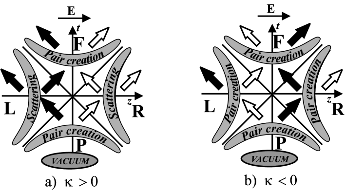
Figure 1: Spacetime location of particle creation regions and direction of particle (empty arrows), antiparticle (filled arrows) fluxes for different signs of $\kappa$.

In $P$- and $F$-wedges the external field creates pairs characterized by $\kappa$ of both signs. The particles created in the $F$ wedge stay within it, while the particles created in the $P$-wedge go to the $R$- and $L$-wedges. If $\kappa>0$, the particles get to the $R$-wedge, while the antiparticles to the $L$-wedge. The incoming particles (antiparticles) are partially reflected there by the effective potential (12) and arrive to the $F$-wedge. Those particles (antiparticles) which penetrate through the potential go to the right infinity of the $R$-wedge (left infinity of the $L$-wedge), where they can be detected by a remote uniformly accelerated (Rindler) observer who is moving along a hyperbolic world line $\rho={\rm const}$. In particular, the Rindler observer in the right wedge will detect created particles and will not observe antiparticles. Since the particles behind the scattering barrier in the $R$-wedge are continuously accelerated by the electric field, they are travelling with almost the speed of light. It is clear that the number of particles with $\kappa>0$ which are crossing the world line of a remote Rindler observer per unit his local time is given by

$$J_{\kappa}=D_{\kappa}n_{\kappa}^{(P)}=e^{-\pi/\mathcal{E}},\quad\kappa>0.$$ (17)

If $\kappa<0$, then the particles created in the wedge $P$ get to the $L$-wedge, while the antiparticles to the $R$-wedge. All of them are reflected by the effective potential (12) and follow to the $F$-wedge. But the electric field creates pairs with $\kappa<0$ directly in the $R$ and $L$ wedges. The particles created in the wedge $R$ (antiparticles in $L$) move to the right (left) spatial infinity, while the antiparticles (particles) go to the $F$-wedge. Hence, independently of the sign of $\kappa$ the right Rindler observer always detects only particles. But if at $\kappa>0$ these particles originate from the $P$-wedge, at $\kappa<0$ they are created at the sub-barrier region in the $R$-wedge itself. The important point is that the number of particles created in the wedge $R$ (and $L$) in the current situation differs from the expression (16) because the latter is related to particle production from vacuum. However, pairs in the wedge $R$ are created in the presence of antiparticles arrived from the $P$-wedge. Since scalar particles satisfy the Bose statistics, presence of antiparticles results in stimulation of pair production in the $R$-wedge. Therefore the number of particles with $\kappa<0$ actually produced in the wedge $R$ and equal to the number of particles detected by the remote Rindler observer per unit his local time is given by (see, e.g., Ref. [10])

$$J_{\kappa}=n_{\kappa}^{(R)}\left(1+n_{\kappa}^{(P)}\right)=e^{-\pi/\mathcal{E}},\quad\kappa<0,$$ (18)

with the quantity $n_{\kappa}^{(R)}$ defined in Eq.(16). Thus, the spectrum of particles measured by the Rindler observer is independent of quantum number $\kappa$.

It is worth noting that this result can also be obtained directly from the solution (5). Indeed, the asymptotic form (6) of this solution can be analytically continued to the right spatial infinity of the $R$-wedge along the path in the complex space $\{x_{+},x_{-}\}$, which goes round the horizon $x_{+}=0$ at sufficiently large distance, such that the semiclassical approximation remains valid along all the path. It is easy to see, that after such continuation the classical action $S_{\kappa}(x_{+},x_{-})$ acquires constant imaginary part $\Delta S_{\kappa}=i\pi/2\,\mathcal{E}$. Since the solution (5) corresponds to an incoming antiparticle at far past in wedge $P$ and antiparticles do not penetrate through the potential $U_{\kappa}$, see Fig. 1, the asymptotic of solution (5) describes at the right spatial infinity of the $R$-wedge only particles created by the electric field. Hence, the asymptotic of the current in this region is equal to $eJ_{\kappa}$ and after simple calculations we arrive to the result $J_{\kappa}=\exp\{-2\,{\rm Im}\,S_{\kappa}\}$ in full agreement with Eqs. (17), (18).

Our analysis can be generalized to the 3-dimensional case. Indeed, it is clear that the 3-dimensional KFG equation after separation of variables orthogonal to the direction of the electric field reduces to the equation for the 1-dimensional problem with the effective mass $\sqrt{m^{2}+p_{\perp}^{2}}$ instead of $m$. Hence the number of particles with quantum numbers $(\kappa,\mathbf{p}_{\perp})$ detected by remote Rindler observer per unit local time $\eta$ can be obtained from Eqs. (17), (18) by substitution $m\rightarrow\sqrt{m^{2}+p_{\perp}^{2}}$

$$J_{\kappa,\mathbf{p}_{\perp}}=\exp\left(-\frac{\pi\left(m^{2}+p_{\perp}^{2}\right)}{eE}\right).$$ (19)

6. Finally, we summarize our results and present the conclusions. In this paper we have analyzed the process of pair creation by a constant homogeneous electric field in MS viewed from a uniformly accelerated reference frame. We have shown that the spectrum of particles (antiparticles) measured by a remote uniformly accelerated observer is precisely the same as the one measured by a conventional inertial observer (see, e.g., Refs. [3, 10]). This means that inertial forces cannot create particles. In particular, no particles can be observed at spatial infinity in the absence of the electric field with respect to both reference frames. In our opinion, this conclusion is an additional explicit demonstration of non-existence of the so-called Unruh effect [8]. Previously, we have come to the same conclusion in Refs. [12, 15, 16] on the basis of quite different arguments.

Let us emphasize that the number of pairs (16) created in the $R$-wedge, when it is considered as a separate spacetime with a special condition imposed at its boundary, is absolutely different from the one (17), (18) measured by a remote uniformly accelerating observer in MS where communication between the wedges is possible. This result provides additional evidence for the necessity of boundary conditions for consistent field quantization on incomplete manifolds, see Refs. [15, 12].

The authors wish to thank L.B. Okun for constant interest to our work. We appreciate support from the Russian Fund for Basic Research and Ministry of Education of Russian Federation.

References

- [1] J. Schwinger, Phys. Rev. 82 (1951) 664.
- [2] A.I. Nikishov, Zh. Eksp. Teor. Fiz. 57 (1969) 1210 (Sov. Phys. JETP 30 (1969) 660).
- [3] N.B. Narozhny, A.I. Nikishov, Yad. Fiz. 11 (1970) 1072 (Sov. Journ. Nucl. Phys. 11 (1970) 596).
- [4] V.S. Popov, Zh. Eksp. Teor. Fiz. 62 (1972) 1248 (Sov. Phys. JETP 35 (1972) 569).
- [5] A.A. Grib, V.M. Mostepanenko, V.M. Frolov, Teor. Mat. Fiz. 13 (1972) 377.
- [6] N.B. Narozhny, A.I. Nikishov, Teor. Mat. Fiz. 26 (1976) 16 (Theor. Math. Phys. 26 (1976) 9).
- [7] N.B. Narozhny, A.I. Nikishov, in Issues in Intense-Field Quantum Electrodynamics, Proc. Lebedev Phys. Inst. Vol. 168, p. 226. Ed. by V.L. Ginzburg (Commack, N.Y. Nova Science, 1987).
- [8] W.G. Unruh. Phys. Rev. D 14 (1976) 870.
- [9] N.D. Birrell and P.C.W. Davies, Quantum Fields in Curved Space (Cambridge University Press, Cambridge, 1982).
- [10] A.I. Nikishov, Issues in Intense-Field Quantum Electrodynamics, Trudy Lebedev Phys. Inst. Vol. 111, (Moskva, Nauka, 1979).
- [11] H. Bateman and A. Erdelyi, Higher Transcendential Functions, Vol. 1 (Mc Graw-Hill, New York, 1953).
- [12] N.B. Narozhny, A.M. Fedotov, B.M. Karnakov, V.D. Mur, and V.A. Belinskii, Phys. Rev. D 65 (2002) 025004.
- [13] O. Klein, Zs. Phys. 53 (1929) 157; F. Sauter, ibid. 69 (1931) 742; 73 (1931) 547; A.I. Nikishov, Nucl. Phys. B21 (1970) 346.
- [14] F. Hund, Zs. Phys. 117 (1940) 1.
- [15] N. Narozhny, A. Fedotov, B. Karnakov, V. Mur, and V. Belinskii, Ann. Phys. (Leipzig) 9 (2000) 199.
- [16] A.M. Fedotov, N.B. Narozhny, V.D. Mur, and V.A. Belinskii, Phys. Lett. A, 305 (2002) 211.