TPI-MINN-02/47, UMN-TH-2120/2

ITEP-TH-21/03, CERN-TH/2003-071

${\cal N}=2$ Sigma Model with Twisted Mass and Superpotential: Central Charges and Solitons

A. Losev^a,b and M. Shifman^b,c

${}^{a}\,$Institute of Theoretical and Experimental Physics,
B. Cheremushkinskaya 25, Moscow 117259, Russia^⋆

${}^{b}\,$William I. Fine Theoretical Physics Institute, University of Minnesota,
116 Church St. S.E., Minneapolis, MN 55455, USA^⋆

${}^{c}\,$Theory Division, CERN
CH-1211 Geneva 23, Switzerland

Abstract

We consider supersymmetric sigma models on the Kähler target spaces, with twisted mass. The Kähler spaces are assumed to have holomorphic Killing vectors. Introduction of a superpotential of a special type is known to be consistent with ${\cal N}=2$ superalgebra (Alvarez-Gaumé and Freedman). We show that the algebra acquires central charges in the anticommutators $\{Q_{L},Q_{L}\}$ and $\{Q_{R},Q_{R}\}$. These central charges have no parallels, and they can exist only in two dimensions. The central extension of the ${\cal N}=2$ superalgebra we found paves the way to a novel phenomenon — spontaneous breaking of a part of supersymmetry. In the general case 1/2 of supersymmetry is spontaneously broken (the vacuum energy density is positive), while the remaining 1/2 is realized linearly. In the model at hand the standard fermion number is not defined, so that the Witten index as well as the Cecotti-Fendley-Intriligator-Vafa index are useless. We show how to construct an index for counting short multiplets in internal algebraic terms which is well-defined in spite of the absence of the standard fermion number. Finally, we outline derivation of the quantum anomaly in the anticommutator $\{\bar{Q}_{L},Q_{R}\}$.

 
^⋆ Permanent address.

1 Introduction

Supersymmetric ${\cal N}=2$ two-dimensional sigma models with twisted mass term possess a variety of central charges and exhibit (see e.g. [1]) nontrivial phenomena similar to those of the Seiberg-Witten theory in four dimensions. It was noted long ago [2] that further deformation of this model by a judiciously chosen superpotential is possible. In this paper we show that such deformation results in emergence of a central charge of a novel type. (A similar algebra was considered previously [3] in a quantum-mechanical context.) As a consequence, ${\cal N}=2$ supersymmetry is spontaneoulsy broken down to ${\cal N}=1$, in defiance of a well-known theorem forbidding this phenomenon. Moreover, Witten’s index [4] turns out to be useless for counting the number of the vacuum states in this case, since it always vanishes. The Cecotti-Fendley-Intriligator-Vafa (CFIV) index [5], $I_{\rm CFIV}={\rm Tr}\,F(-1)^{F}\,,$ which might be appropriate for counting vacua (rather than BPS solitons!), does not work in this model either, since the standard definition of the fermion number does not work. We show how new indices, ${\cal I}_{2,1/2}$ and ${\cal I}_{2,1/4}$ (formulated in internal algebraic terms) replacing that of CFIV, can be introduced following the line of reasoning of Ref. [6]. The index ${\cal I}_{2,1/2}$ counts the number of 1/2 BPS-saturated vacua, while ${\cal I}_{2,1/4}$ counts the number of 1/4 BPS-saturated kinks.

In the simplest example including twisted mass and superpotential we find explicit 1/4 BPS kink solutions. Derivation of anomaly in the central charges is outlined.

2 Sigma model and twisted mass

Two-dimensional sigma models with twisted mass were first constructed in Ref. [2]. The superspace/superfield description was developed in Refs. [7, 8]. In particular, the notion of a twisted chiral superfield was introduced in the second of these works . Our task in this section is to briefly review introduction of the twisted mass $m$ in the sigma model of a general form and set the notation to be used throughout the paper.

For Kähler target space endowed with the metric $G_{\bar{j}\,i}$ the Lagrangian of the undeformed (i.e. $m=0$) model is

$${\cal L}_{0}=G_{\bar{j}\,i}\,\partial^{\mu}\bar{\phi}^{\,\bar{j}}\,\partial_{\mu}\phi^{i}+\frac{i}{2}G_{\bar{j}\,i}\,\bar{\Psi}^{\bar{j}}\!\stackrel{{\scriptstyle\leftrightarrow}}{{\not\!\!D}}\Psi^{i}+R_{\bar{j}ik\bar{l}}\,\bar{\Psi}_{L}^{\,\bar{j}}\Psi_{L}^{i}\Psi_{R}^{k}\bar{\Psi}_{R}^{\,\bar{l}}\,,$$ (2.1)

where $D_{\mu}$ is the covariant derivative,

$$D_{\mu}\,\Psi^{i}=\partial_{\mu}\,\Psi^{i}+\partial_{\mu}\phi^{k}\,\Gamma_{kl}^{i}\,\Psi^{l}\,.$$ (2.2)

Here $\Gamma$’s stand for the Christoffel symbols, $R_{\bar{j}ik\bar{l}}$ is the curvature tensor, while $\Psi$ denotes a two-component spinor,

$$\Psi=\left(\begin{array}[]{cc}\Psi_{R}\\ \Psi_{L}\end{array}\right),$$ (2.3)

so that the kinetic term of the fermions can be identically rewritten as

$$\frac{i}{2}G_{i\bar{j}}\,\bar{\Psi}^{\bar{j}}\!\stackrel{{\scriptstyle\leftrightarrow}}{{\not\!\!D}}\Psi^{i}=\frac{i}{2}G_{i\bar{j}}\left\{\bar{\Psi}_{L}^{\bar{j}}\!\stackrel{{\scriptstyle\leftrightarrow}}{{\not\!\!D}}_{R}\Psi_{L}^{i}+\bar{\Psi}_{R}^{\bar{j}}\!\stackrel{{\scriptstyle\leftrightarrow}}{{\not\!\!D}}_{L}\Psi_{R}^{i}\right\}\,.$$ (2.4)

The right and left derivatives are defined in Eq. (4.2).

In addition, one can introduce a $\theta$ term which has the following general form

$${\cal L}_{\theta}=\frac{i\theta}{2\pi}\,B_{i\bar{j}}\,\varepsilon^{\mu\nu}\partial_{\mu}\bar{\phi}^{\,\bar{j}}\partial_{\nu}\phi^{i}\,,$$ (2.5)

where $B_{i\bar{j}}$ is a closed 2-form (i.e. $\partial_{k}B_{i\bar{j}}=\partial_{i}B_{k\bar{j}}$ and h.c.). For the particular example of the CP(1) model, to be discussed in some detail below, $B_{i\bar{j}}$ can be chosen proportional to the round metric $G_{i\bar{j}}=\delta_{i\bar{j}}(1+|\phi|^{2})^{-2}$.

If the target space of the ${\cal N}=2$ sigma model (2.1) has isometries, one can carry out [2] a mass deformation of the model, by introducing the so-called twisted mass, without breaking ${\cal N}=2$. Suppose $V=\{v^{i}\,,\,\,\bar{v}^{\,\bar{j}}\}$ is a holomorphic vector field, i.e. $v^{i}=v^{i}(\phi)$, $\bar{v}^{\,\bar{j}}=\bar{v}^{\,\bar{j}}(\bar{\phi})$ and the Lie derivative ${\cal L}_{V}$ annihilates the metric,

$${\cal L}_{V}G_{\bar{j}\,i} \equiv {\cal L}_{v}G_{\bar{j}\,i}+{\cal L}_{\bar{v}}G_{\bar{j}\,i}=0\,;$$

$${\cal L}_{v}G_{\bar{j}\,i} \equiv v^{k}\partial_{k}G_{\bar{j}\,i}+\partial_{i}\,v^{k}G_{\bar{j}\,k}\,;$$

$${\cal L}_{\bar{v}}G_{\bar{j}\,i} \equiv \bar{v}^{\,\bar{k}}\partial_{\bar{k}}G_{\bar{j}\,i}+\partial_{\bar{j}}\bar{v}^{\,\bar{k}}G_{\bar{k}\,i}\,.$$ (2.6)

Then the twisted mass term takes the form

$${\cal L}_{m}=\left(m\bar{m}\right)\,G_{\bar{j}\,i}\,\bar{v}^{\,\bar{j}}\,v^{i}-m\left({\cal L}_{v}G_{\bar{j}\,i}\right)\bar{\Psi}_{L}^{\,\bar{j}}\Psi_{R}^{i}+\bar{m}\left({\cal L}_{\bar{v}}G_{\bar{j}\,i}\right)\bar{\Psi}_{R}^{\,\bar{j}}\Psi_{L}^{i}\,,$$ (2.7)

where $m$ is a complex parameter. Note that Eq. (2.7) is invariant under vector rotations of the fermion fields, $\Psi_{L,R}\to\exp(i\alpha)\Psi_{L,R}$. The corresponding charge can be viewed as a fermion number. The axial transformation of the fermion fields, $\Psi_{L}\to\exp(i\alpha)\Psi_{L}$, $\Psi_{R}\to\exp(-i\alpha)\Psi_{R}$, allows one to rotate away the phase of $m$ at a price of redefining the $\theta$ angle.

The easiest way to derive Eq. (2.7) is to choose the coordinate frame $\Phi^{j}$ ($j=0,1,...,n$) in such a way that

$$v^{j}=iv_{0}\,\delta^{0j}\,,\qquad v_{0}={\rm real\,\,\,const}\,.$$ (2.8)

Below the coordinates $\Phi_{0},\,\,\bar{\Phi}_{0}$ will be referred to as special. With this choice, the Kähler term

$$\int d^{4}\theta K\left(\Phi_{0}+\bar{\Phi}_{0}+2\bar{m}\theta_{L}\bar{\theta}_{R}+2m\theta_{R}\bar{\theta}_{L}\right)$$ (2.9)

leads to ${\cal N}=2$ preserving sigma model with the twisted mass.

The choice of the coordinates in Eqs. (2.1) and (2.7) is different from the special one. Here the coordinates $\phi\,,\,\,\bar{\phi}$ are such that the Kähler potential $K$ depends on the product $\bar{\phi}\phi$, so that the model is invariant under phase rotations

$$\phi\to\phi\,e^{i\alpha}\,,\qquad\bar{\phi}\to\bar{\phi}\,e^{-i\alpha}\,.$$ (2.10)

The special coordinates are related to $\phi\,,\,\,\bar{\phi}$ through the transformation

$$\phi=e^{\Phi_{0}}\,,\quad\phi_{j}=\Phi_{j}\,,\quad j>0\,.$$

3 Introduction of superpotential

The question is whether one can introduce a superpotential in the model with the twisted mass without breaking ${\cal N}=2$. It is clear that a generic superpotential destroys isometry of the target space; in this case combining the twisted mass with a superpotential breaks ${\cal N}=2$ explicitly. One can find, however, a special superpotential [2] preserving the isometry. In the special coordinates it has the form

$$d{\cal W}=w\,d\Phi_{0}\,,$$ (3.1)

($w$ is a complex constant) which is invariant under shifts of $\Phi_{0}$ (cf. Eq. (2.8)). Then in the coordinates used in Eqs. (2.1) and (2.7)

$$d{\cal W}=w\,\frac{d\phi}{\phi}\,.$$ (3.2)

Note that the superpotential ${\cal W}=w\,\ln\phi$ is multivalued – this feature is unavoidable. This causes no problems, however, since $d{\cal W}$ is well-defined, and this is all we need. It is worth mentioning that such multivalued superpotentials appeared previously [9] in the context of the Kähler sigma models in the mirror descriptions of the projective spaces with twisted mass term.

The superpotential enters through $F$ term. This generates the following additional term in the Lagrangian

$${\cal L}_{F}=-G^{\,i\,\bar{j}}\left(\partial_{i}{\cal W}\right)\left(\partial_{\bar{j}}\,\bar{\cal W}\right)-\left\{\left(D_{i}\partial_{j}{\cal W}\right)\Psi_{R}^{j}\Psi_{L}^{i}+\mbox{h.c.}\right\}\,.$$ (3.3)

Assembling Eqs. (2.1), (2.7) and (3.3) we get the full Lagrangian of the deformed model.

Note that the second term in Eq. (3.3) forbids the vector transformation of the fermion field. On the other hand, the fermion mass term in Eq. (2.7) forbids the axial transformation. Thus, the standard fermion number is not defined in the model including both twisted mass term and superpotential. A U(1) symmetry involving both fermion and boson fields does exist, however; the Lagrangian (2.1), (2.7) and (3.3) is invariant under

$$\Psi_{L,R} \to \Psi_{L,R}\,e^{i\alpha}\,,\qquad\phi\to\phi\,e^{i\alpha}\,;$$

$$\bar{\Psi}_{L,R} \to \bar{\Psi}_{L,R}\,e^{-i\alpha}\,,\qquad\bar{\phi}\to\bar{\phi}\,e^{-i\alpha}\,.$$ (3.4)

The corresponding conserved current is 

$${\cal J}^{\mu}_{\rm U(1)} = G_{\bar{j}\,i}\left(\bar{\phi}^{\bar{j}}\,i\stackrel{{\scriptstyle\leftrightarrow}}{{\partial}}^{\,\mu}\!\phi^{i}+\bar{\Psi}^{\bar{j}}\gamma^{\mu}\Psi^{i}\right)+\frac{1}{2}\left(\bar{\phi}^{\bar{i}}\bar{\Psi}^{\bar{j}}\gamma^{\mu}\Psi^{i}\bar{\Gamma}_{\bar{i}\bar{j}}^{\bar{k}}G_{i\bar{k}}+\phi^{i}\bar{\Psi}^{\bar{i}}\gamma^{\mu}{\Psi}^{j}\Gamma_{ij}^{k}G_{k\bar{i}}\right),$$

$$\qquad q_{\rm U(1)} \equiv \int dx{\cal J}^{0}_{\rm U(1)}\,.$$ (3.5)

4 Superalgebra

As was mentioned, the model given by Eqs. (2.1), (2.7), (3.3) is ${\cal N}=2$ supersymmetric, i.e. possesses four conserved supercharges. The superalgebra emerging after inclusion of the superpotential is rather peculiar, however: it contains a central charge of the type which seems to escape theorists’ attention previously. Here we will discuss it in some detail.

The easiest way to derive the corresponding superalgebra at tree level (we will discuss possible anomalies in Sect. 10) is to consider the model in the flat limit, i.e. $G_{\bar{j}\,i}=1$. Moreover, for our present purposes we may drop target space indices ${\bar{j}\,,\,i}$ limiting ourselves to one (complex) field.

Then the conserved supercharges are

$$Q_{R} = \int dx\left\{\left(\partial_{R}\bar{\phi}\right)\Psi_{R}+i\bar{m}\bar{\phi}\Psi_{L}-i\frac{\bar{w}}{\bar{\phi}}\bar{\Psi}_{L}\right\}\,,$$

$$\bar{Q}_{R} = \int dx\left\{\left(\partial_{R}\phi\right)\bar{\Psi}_{R}-im\phi\bar{\Psi}_{L}+i\frac{w}{\phi}\Psi_{L}\right\}\,;$$

$$Q_{L} = \int dx\left\{\left(\partial_{L}\bar{\phi}\right)\Psi_{L}+im\bar{\phi}\Psi_{R}+i\frac{\bar{w}}{\bar{\phi}}\bar{\Psi}_{R}\right\}\,,$$

$$\bar{Q}_{L} = \int dx\left\{\left(\partial_{L}\phi\right)\bar{\Psi}_{L}-i\bar{m}\phi\bar{\Psi}_{R}-i\frac{w}{\phi}\Psi_{R}\right\}\,,$$ (4.1)

where

$$\partial_{R}=\partial_{0}-\partial_{1}\,,\qquad\partial_{L}=\partial_{0}+\partial_{1}\,.$$ (4.2)

Needless to say that all supercharges are neutral with respect to $q_{\rm U(1)}$.

The following superalgebra ensues:

$$\{\bar{Q}_{L},Q_{L}\} = H+P\,,\quad\{\bar{Q}_{R},Q_{R}\}=H-P\,;$$ (4.3)

$$\{Q_{L},\bar{Q}_{R}\} = mq_{\rm U(1)}-im\,\int dx\,\partial_{x}\,h\,,$$ (4.4)

$$\{Q_{R},\bar{Q}_{L}\} = \bar{m}q_{\rm U(1)}+i\bar{m}\,\int dx\,\partial_{x}\,h\,;$$ (4.5)

$$\{Q_{R},Q_{R}\} = 2\bar{m}\,\bar{w}\int dx\,,\qquad\{\bar{Q}_{R},\bar{Q}_{R}\}=2m\,w\int dx\,;$$ (4.6)

$$\{Q_{L},Q_{L}\} = -2m\bar{w}\int dx\,,\qquad\{\bar{Q}_{L},\bar{Q}_{L}\}=-2\bar{m}\,w\int dx\,;$$ (4.7)

$$\{Q_{L},Q_{R}\} = -2i\,\bar{w}\int dx\,\partial_{x}\,\ln\bar{\phi}\,,\qquad\{\bar{Q}_{L},\bar{Q}_{R}\}=2i\,w\int dx\,\partial_{x}\,\ln\phi\,,$$ (4.8)

where $(H,P)$ is the energy-momentum operator,

$$(H,P)=\int dx\theta^{0\mu}\,,\qquad\mu=0,1\,,$$

and $\theta^{\mu\nu}$ is the energy-momentum tensor. Finally, the function $h$ in Eqs. (4.4), (4.5) is

$$h=\phi\bar{\phi}\,.$$ (4.9)

(The function $h$ is sometimes called “the hamiltonian of the isometry.” Indeed, if we formally consider the Kähler target space as a symplectic manifold, i.e. as a phase space, with the symplectic form $\Omega$ being the Kähler form,

$$\Omega=-id\phi\wedge d\bar{\phi}$$

in our example, and view $h$ as a “hamiltonian,” then the isometry transformations become a dynamical flow on the phase space,

$$\partial_{\bar{j}}h=v^{i}\Omega_{i\bar{j}},\qquad\partial_{i}h=-\bar{v}^{\bar{j}}\Omega_{i\bar{j}}\,.$$

Warning: the function $h$ has nothing to do with the energy operator $H$ above.)

Equation (4.9) is specific for flat metric. Introduction of a nontrivial Kähler metric modifies the expressions for supercharges, e.g.

$$Q_{R}=\int dx\left\{G\left[\left(\partial_{R}\bar{\phi}\right)\Psi_{R}+i\bar{m}\bar{\phi}\Psi_{L}\right]-i\frac{\bar{w}}{\bar{\phi}}\bar{\Psi}_{L}\right\},$$ (4.10)

and so on. This entails, in turn, that the hamiltonian of the isometry $h$ must be modified appropriately too, see e.g. Sect. 7 where we treat the example of the $C^{*}$ model, a “relative” of CP(1). Equations (4.3) through (4.8) are valid in the general case, for arbitrary metric $G_{\bar{j}\,i}$, not only for the flat metric. Equations (4.4) and (4.5) get extended by anomalous terms, to be discussed in Sect. 10. A novel feature which we would like to stress is the occurrence of central charges in Eqs. (4.6) and (4.7) that do not vanish if and only if both twisted mass and superpotential are present. Note that they are proportional to the spatial size of the system. Therefore, they are relevant to vacua rather than to BPS solitons, as is the case for all other central charges.

5 Implications for vacua

In this section we will discuss implications of the algebra (4.3) — (4.8). For the time being we are interested in the structure of the vacuum states rather than in solitons. Therefore, we will switch off all topological charges in Eqs. (4.4), (4.5) and (4.8). In addition we will set $q_{\rm U(1)}=0$. Our focus is the novel central charge induced by combining twisted mass and superpotential, Eqs. (4.6) and (4.7).

For what follows it is convenient to introduce two phases

$$e^{i\beta_{R}}=-\frac{|w/\bar{m}|}{w/\bar{m}}\,,\qquad e^{i\beta_{L}}=\frac{|w/m|}{w/m}\,.$$ (5.1)

Suppose we are interested in the vacuum states, i.e. terms with derivatives in the expressions for supercharges can be discarded. It is not difficult to see that the following two supercharges

$$Q_{3}=e^{-i\beta_{R}/2}Q_{R}+e^{i\beta_{R}/2}\,\bar{Q}_{R}\quad\mbox{and}\quad Q_{4}=e^{-i\beta_{L}/2}Q_{L}+e^{i\beta_{L}/2}\,\bar{Q}_{L}$$ (5.2)

annihilate the vacua, $Q_{3,4}|\rm vac\rangle=0$. Moreover,

$$Q_{3}^{2}=Q_{4}^{2}=H-|Z|\,,$$ (5.3)

where

$$|Z|=2L|wm|\,,$$ (5.4)

and $L$ is the spatial size of the system. The supercharges $Q_{3,4}$ (as well as $Q_{1,2}$ below) are defined in such a way that they are Hermitean.

As was repeatedly mentioned, in the general case the only constraint on the metric is as follows: the Kähler potential we deal with must be invariant under the phase rotation of the fields $\phi,\,\,\bar{\phi}$, see Eq. (3.4). A generic potential invariant under these rotations has the form

$$K(\phi^{i}\,,\,\,\overline{\phi^{j}})=K(\phi^{i}\overline{\phi^{j}})\,.$$ (5.5)

For instance, the Kähler potential of the CP($N-1$) model,

$$K_{{\rm CP}(N-1)}=\ln\left(1+\sum_{i=1}^{N-1}|\phi^{i}|^{2}\right)\,,$$

does the job. Needless to say that the metric

$$G_{i\bar{j}}=\frac{\partial}{\partial\phi^{i}}\,\frac{\partial}{\partial\bar{\phi}^{\,\bar{j}}}\,K(\phi\bar{\phi})$$

is then also invariant. If we have a single field $\phi$ (and its complex-conjugated $\bar{\phi}$)

$$G_{\bar{j}\,i}\to G(\bar{\phi}\phi)\,.$$

where we assume $G$ to be positive. It is obtained from the Kähler potential $K(\phi\bar{\phi})$ as follows:

$$G(x)=K^{\prime}(x)+xK^{\prime\prime}(x)\,,\qquad x=\phi\bar{\phi}.$$

Then the vacuum value of the field $\phi$ is

$$\phi_{\rm vac}=f_{0}\,\,e^{i\alpha}\,,$$ (5.6)

where the parameter $f_{0}$ is any positive root of the equation

$$f^{2}=\left|\frac{w}{m}\right|\,\frac{1}{G(f^{2})}\,.$$ (5.7)

The phase $\alpha$ is arbitrary. In other words, we find a continuous compact vacuum manifold (see Fig. 1). The number of positive roots of Eq. (5.7) mod 2 is a topological invariant related to the index introduced in Sect. 6.

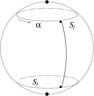
Figure 1: The vacuum manifold in the simplest model with twisted mass and superpotential, see (7.1). The target space is $S_{2}$ with the punctured poles (the poles are marked by closed circles). The vacuum manifold consists of two disconnected $S_{1}$ submanifolds. The trajectory running along a meridian and interpolating between vacua belonging to the first and second $S_{1}$ respectively (thick solid line) is a 1/4 BPS saturated kink.

Equation (5.7) is obtained by requiring $Q_{3}$ (or $Q_{4}$) to annihilate vacuum. The vacuum fields $\phi_{\rm vac},\,\,\bar{\phi}_{\rm vac}$ are coordinate-independent; therefore, all terms with derivatives in Eq. (4.10) and similar for $\bar{Q}_{R}$ can be dropped. The very same equation (5.7) is obtained through Bogomolny completion of the potential term in the Hamiltonian,

$${\cal E}=G\left(\bar{m}\bar{\phi}+e^{i\beta_{R}}\,G^{-1}\,\frac{w}{\phi}\right)\left(m\phi+e^{-i\beta_{R}}\,G^{-1}\,\frac{\bar{w}}{\bar{\phi}}\right)+2|wm|\,.$$

Equations (5.6) and (5.7) assume that $P_{\rm vac}=0$. The ground state energy density ${\cal E}_{\rm vac}$ is

$${\cal E}_{\rm vac}=2|mw|\neq 0\,.$$ (5.8)

Normally this would signal spontaneous breaking of all four supercharges. The well-known theorem reads that in extended supersymmetries one cannot break spontaneously a part of it: ${\cal E}_{\rm vac}\neq 0$ necessarily implies that all supercharges are broken. However, in our case the unconventional central extension of superalgebra, Eqs. (4.6) and (4.7), invalidates this theorem. Thus, in the sigma model with twisted mass and superpotential, ${\cal N}=2$ symmetry is spontaneosly broken down to ${\cal N}=1$ provided that Eq. (5.7) has at least one positive root. (It can have more than one root, though.)

Now, it is instructive to consider two remaining combinations of the supercharges — those orthogonal to $Q_{3,4}$,

$$Q_{1}=i\left(e^{-i\beta_{R}/2}Q_{R}-e^{i\beta_{R}/2}\,\bar{Q}_{R}\right)\quad\mbox{and}\quad Q_{2}=i\left(e^{-i\beta_{L}/2}Q_{L}-e^{i\beta_{L}/2}\,\bar{Q}_{L}\right).$$ (5.9)

They do not annihilate the vacuum state since

$$Q_{1}^{2}=Q_{2}^{2}=H+|Z|\,.$$ (5.10)

Rather, acting on vacuum, they produce Goldstino,

$$\psi_{\rm G}=\frac{1}{\sqrt{2}}\,\left(\begin{array}[]{c}e^{-i\gamma_{R}}\Psi_{R}+e^{i\gamma_{R}}\bar{\Psi}_{R}\\[8.53581pt] e^{-i\gamma_{L}}\Psi_{L}+e^{i\gamma_{L}}\bar{\Psi}_{L}\end{array}\right),$$ (5.11)

where 

$$\gamma_{R}=\frac{\beta_{L}}{2}+\alpha-\mbox{arg}\,(m)\,,\qquad\gamma_{L}=\frac{\beta_{R}}{2}+\alpha+\mbox{arg}\,(m)\,.$$ (5.12)

The Goldstino field is a Majorana field which pairs up with the massless scalar corresponding to the would-be Goldstone boson of U(1) to form a massless ${\cal N}=1$ supermultiplet. (The above massless scalar is in fact the phase of $\phi$.) The second Majorana spinor field, orthogonal to (5.11),

$$\psi_{m}=\frac{i}{\sqrt{2}}\,\left(\begin{array}[]{c}e^{-i\gamma_{R}}\Psi_{R}-e^{i\gamma_{R}}\bar{\Psi}_{R}\\[8.53581pt] e^{-i\gamma_{L}}\Psi_{L}-e^{i\gamma_{L}}\bar{\Psi}_{L}\end{array}\right),$$ (5.13)

pairs up with the remaining massive scalar field to form the second ${\cal N}=1$ supermultiplet, with mass $\neq 0$. If we parametrize $\phi=f_{0}+2^{-1/2}(\sigma+i\rho)$, then the quadratic part of the Lagrangian takes the form

$${\cal L}^{(2)} = \frac{1}{2}\,G(f_{0}^{2})\left(\partial_{\mu}\sigma\,\partial^{\mu}\sigma-\tilde{m}^{2}\sigma^{2}+\bar{\psi}_{m}\not\!\partial\,\psi_{m}-\tilde{m}\bar{\psi}_{m}\psi_{m}\right.$$ (5.14)

$$+ \left.\partial_{\mu}\rho\,\partial^{\mu}\rho+\bar{\psi}_{\rm G}\not\!\partial\,\psi_{\rm G}\right)\,,$$

where

$$\tilde{m}=|m|\,\left|2+f\frac{\partial}{\partial f}\,\ln\,G\right|_{f=f_{0}}\,.$$ (5.15)

Let us parenthetically note that in the model (7.1)

$$\tilde{m}=2|m|\,\frac{\sqrt{\beta^{2}-1}}{\beta}\,,$$ (5.16)

where the parameter $\beta$ is defined in Eq. (7.9).

If Eq. (5.7) has no positive roots, all four supercharges act on the vacuum nontrivially. Then ${\cal N}=2$ supersymmetry is completely spontaneously broken.

6 Counting vacua and kinks, or what replaces the CFIV index

As was explained above, the fermion charge is not defined in the model at hand. Of course, the fermion parity $(-1)^{F}$ remains well-defined (the latter is in contradistinction to what happens [6] in ${\cal N}=1$ models).

The absence of the fermion number precludes us from using the CFIV index. However, since ${\cal N}=2$ superalgebra remains valid (albeit centrally extended), there should exist an index replacing the CFIV index. The replacement must be formulated exclusively in internal algebraic terms, as was done in Ref. [6] that treated ${\cal N}=1$ two-dimensional models where neither $F$ nor $(-1)^{F}$ was defined for BPS states.

Here we suggest indices for counting 1/2 BPS-saturated states (vacua) and 1/4 BPS-saturated states (kinks) in the problem at hand (centrally extended ${\cal N}=2$). Our construction is a direct generalization of that of Ref. [6].

6.1 A brief reminder of the ${\cal N}=1$ story

In the ${\cal N}=1$ case we study the representations of the superalgebra

$$Q_{1}^{2}=H+Z\,,\qquad Q_{2}^{2}=H-Z\,,$$ (6.1)

where $Z$ is assumed to be positive.

For non-BPS states, $H>Z$, the representation is obviously two-dimensional. Each supermultiplet is a doublet. The BPS states correspond to one-dimensional representations of the algebra which can be of two types, $v_{\pm}$, such that

$$Q_{2}\,v_{\pm}=0\,,\qquad Q_{1}\,v_{\pm}=\pm\sqrt{2Z}\,v_{\pm}\,.$$ (6.2)

The index is the difference between the numbers of the BPS states with the positive and negative eigenvalues of $Q_{1}$. Note, that if the fermion parity $(-1)^{F}$ is a symmetry of the theory, then the above index necessarily vanishes. By fermion parity we mean an operator such that

$$(-1)^{F}\,Q_{i}\,(-1)^{F}=-Q_{i}\,,\qquad i=1,2\,.$$ (6.3)

Indeed, assume we have a state $v_{+}$. Then the state $(-1)^{F}v_{+}$ is in fact $v_{-}$,

$$Q_{1}\left\{(-1)^{F}\,v_{+}\right\}=(-1)^{F}\left(-Q_{1}\right)v_{+}=-\sqrt{2Z}\left\{(-1)^{F}\,v_{+}\right\}\,.$$ (6.4)

In other words, the existence of $(-1)^{F}$ implies that the states appear in pairs $v_{+},\,\,v_{-}$.

For a generic representation (which can be reducible) the proper index can be introduced as follows:

$${\cal I}_{1}={\rm Tr}\,\frac{Q_{1}}{\sqrt{2Z}}\exp{(-t\,Q_{2}^{2})}\,.$$ (6.5)

From this expression it is clear that the index ${\cal I}_{1}$, being an integer and a smooth function of the parameters of the system, is constant on the space of parameters of the system. For short (one-dimensional) multiplets the value of ${\cal I}_{1}$ is $\pm 1$. For long multiplets ${\cal I}_{1}=0$.

6.2 Counting 1/2 BPS states in ${\cal N}=2$ SUSY

The 1/2 BPS-saturated states in ${\cal N}=2$ SUSY appear when superalgebra takes the form

$$Q_{1}^{2}=Q_{2}^{2}=H+|Z|\,,\qquad Q_{3}^{2}=Q_{4}^{2}=H-|Z|\,,$$ (6.6)

(cf. Eqs. (5.3) and (5.10)). This algebra has four-dimensional irreducible representations — these are long non-BPS representations with $H>|Z|$. If $H=|Z|$ the irreducible representations are short, two-dimensional supermultiplets of the BPS-saturated states.

Cecotti et al. proposed [5] an index,

$$I_{\rm CFIV}={\rm Tr}\,F(-1)^{F}e^{-t(H-|Z|)}\,,$$ (6.7)

which is integer-valued, saturated by short multiplets, and smoothly depends on parameters of the system — thus, it is constant on the space of parameters . However, it requires the existence of a conserved fermion number $F$ with the appropriate commutation relations. In our theory we do not have this luxury. In the case under consideration we do have the conserved fermion parity $(-1)^{F}$. Therefore, we suggest to replace $I_{\rm CFIV}$ by a new index ${\cal I}_{2,1/2}$ defined as follows:

$${\cal I}_{2,1/2}=\frac{1}{2}\,{\rm Tr}\,(-1)^{F}\,\frac{i\,Q_{1}Q_{2}}{2|Z|}\,e^{-t(H-|Z|)}\,.$$ (6.8)

The meaning of the above index is easy to assess. Again, as in Sect. 6.1, there are two types of BPS states, $v_{\pm}$ (now both $v_{+}$ and $v_{-}$ are in fact doublets, say, $v_{+,\alpha}$, where $\alpha=1,2$; we suppress the $\alpha$ index for brevity). The states $v_{\pm}$ can be defined through the relation 

$$i\,Q_{1}Q_{2}\,v_{\pm}=\pm\,2|Z|\,(-1)^{F}\,v_{\pm}\,.$$ (6.9)

Then, the index (6.8) obviously counts the difference between the number of the BPS doublets $v_{+}$ and that of $v_{-}$’s. Long multiplets necessarily consist of pairs $\{v_{+}\,,\,\,v_{-}\}$; hence for long multiplets ${\cal I}_{2,1/2}$ vanishes.

6.3 Counting 1/4 BPS states in ${\cal N}=2$ SUSY

1/4 BPS saturated states in the model under consideration are kinks, to be discussed in Sect. 8. There are four distinct central charges in the corresponding superalgebra presented in Eqs. (8.8) through (8.11). In the 1/4 BPS kink sector we loose $(-1)^{F}$. If the theory is regularized in the infrared, see the previous footnote, one can say that short 1/4 BPS-saturated multiplets are doublets, while long multiplets are quadruplets. This follows from the algebra (8.8) through (8.11), with $Q_{4}=0$ on the BPS states, and all four supercharges operative for non-BPS states.

From the algebraic standpoint the fact that the short kink multiplets are two-dimensional is perfectly obvious. However, it is instructive to ask a physical question: “what is the multiplicity of the kink particles?” The point is that, as has been just mentioned in Sect. 6.2, double degeneracy is the intrinsic property of the 1/2 BPS-saturated vacua. It is this double degeneracy that is inherited by the 1/4 BPS kink multiplets. If we consider kinks interpolating between specific given vacua, then they are unique. Therefore, kinks considered as particles, form one-dimensional representations of superalgebra, see Sect. 8.

Returning to superalgebra (8.8) through (8.11), one can define two types of the BPS states as follows:

$$i\,Q_{1}\,Q_{2}\,Q_{3}\,v_{\pm}=\pm\sqrt{(Z_{4}+Z_{1})(Z_{4}+Z_{2})(Z_{4}-Z_{3})}\,v_{\pm}\,.$$ (6.10)

Then

$${\cal I}_{2,1/4}=\frac{1}{2}\,{\rm Tr}\,\frac{i\,Q_{1}Q_{2}Q_{3}}{\sqrt{(Z_{4}+Z_{1})(Z_{4}+Z_{2})(Z_{4}-Z_{3})}}\,\,e^{-tQ_{4}^{2}}$$ (6.11)

is the desirable index counting the difference between the numbers of $v_{+}$ and $v_{-}$.

Note, that the index ${\cal I}_{2,1/4}$, just like its ${\cal N}=1$ counterpart (see Eq. (6.5)), can be nonvanishing only if the fermion parity is broken. Indeed, if the fermion parity is defined, $(-1)^{F}Q_{i}(-1)^{F}=-Q_{i}\,\quad i=1,...,4,$ then $v_{+}$ and $v_{-}$ appear in pairs $\{v_{-},\,\,v_{+}\}$,

$$v_{-}=(-1)^{F}v_{+}\,.$$

7 Showcase example of $C^{*}$ model (descendant of CP(1))

Here we briefly illustrate our construction starting from the simplest and the most popular ${\cal N}=2$ sigma model, CP(1). We deform this model by adding twisted mass and superpotential, following the strategy outlined in Sect. 2. The CP(1) model is the sigma model on the two-dimensional sphere. It is described by one complex field $\phi$ and one complex two-component spinor $\Psi$. The corresponding Lagrangian is obtained from Eq. (2.1) by dropping the indices $i$ and $\bar{j}$. The target space of the deformed model has the topology of cylinder; the model is referred to as the $C^{*}$ model.

The Lagrangian including twisted mass and superpotential can be written as

$${\cal L}_{\,C^{*}} = G\,\left\{\partial_{\mu}\bar{\phi}\partial^{\mu}\phi-|m|^{2}\,{\phi\bar{\phi}}\right.$$ (7.1)

$$+ \frac{i}{2}\left(\bar{\Psi}_{L}\stackrel{{\scriptstyle\leftrightarrow}}{{\partial_{R}}}\Psi_{L}+\bar{\Psi}_{R}\stackrel{{\scriptstyle\leftrightarrow}}{{\partial_{L}}}\Psi_{R}\right)-\frac{1-\bar{\phi}\phi}{\chi}\left(m\bar{\Psi}_{L}\Psi_{R}+\bar{m}\bar{\Psi}_{R}\Psi_{L}\right)$$

$$- \frac{i}{\chi}\,\left.\left[\bar{\Psi}_{L}\Psi_{L}\left(\bar{\phi}\stackrel{{\scriptstyle\leftrightarrow}}{{\partial_{R}}}\phi\right)+\bar{\Psi}_{R}\Psi_{R}\left(\bar{\phi}\stackrel{{\scriptstyle\leftrightarrow}}{{\partial_{L}}}\phi\right)\right]-\frac{2}{\chi^{2}}\bar{\Psi}_{L}\Psi_{L}\bar{\Psi}_{R}\Psi_{R}\right\}$$

$$- G^{-1}|w|^{2}\,\frac{1}{\bar{\phi}\phi}+\left\{\frac{1-\bar{\phi}\phi}{\chi}\,\,\frac{w}{\phi^{2}}\,\Psi_{R}\Psi_{L}+\mbox{h.c.}\right\}$$

$$+ \frac{i\theta}{2\pi}\,\frac{1}{\chi^{2}}\,\varepsilon^{\mu\nu}\partial_{\mu}\bar{\phi}\partial_{\nu}\phi\,,$$

where the metric $G$

$$G \equiv \frac{2}{g^{2}}\,{\cal G}=\frac{2}{g^{2}}\,\frac{1}{(1+\phi\bar{\phi})^{2}}\,,$$

$${\cal G} = \frac{1}{\chi^{2}}\,,\quad\chi\equiv 1+\phi\bar{\phi}\,.$$ (7.2)

The target space is $S_{2}$. Note that the only nonvanishing Christoffel symbols are

$$\Gamma=-2\,\frac{\bar{\phi}}{\chi}\,,\qquad\bar{\Gamma}=-2\,\frac{\phi}{\chi}\,,$$ (7.3)

while the Ricci tensor in the case at hand is related to the metric as follows

$$R=2\,{\cal G}=\frac{2}{\chi^{2}}\,.$$ (7.4)

The scalar curvature ${\cal R}$ is the inverse radius squared of the target space sphere, ${\cal R}={g^{2}}\,.$ The vector fields on the CP(1) target space are

$$v=\phi,\qquad\bar{v}=-\bar{\phi}\,.$$ (7.5)

Thanks to the existence of this isometry one can introduce twisted mass which breaks O(3) of the undeformed model down to U(1). Besides twisted mass we add a superpotential term preserving U(1) and ${\cal N}=2$ supersymmetry; it is given in the last but one line of Eq. (7.1). The last line is the $\theta$ term. The conserved supercurrent has the form

$$J^{\mu}=\left(\partial_{\lambda}\bar{\phi}\right)\gamma^{\lambda}\gamma^{\mu}\Psi-i\,\bar{m}\,\bar{\phi}\,\gamma^{\mu}\,\Psi+i\frac{\bar{w}}{\bar{\phi}}\,\gamma^{\mu}\Psi^{\dagger}\,.$$ (7.6)

Finally, we have to specify the “hamiltonian” $h$ in Eqs. (4.4) and (4.5),

$$h=\frac{2}{g^{2}}\,\frac{\bar{\phi}\phi}{1+\bar{\phi}\phi}\,.$$ (7.7)

Alternatively the “hamiltonian” can be rewritten as $h=-(2/g^{2})(1+\bar{\phi}\phi)^{-1}$. The vacuum manifold consists of two disconnected $S_{1}$’s (Fig. 1),

$$\phi_{\rm vac}=\left(\beta\pm\sqrt{\beta^{2}-1}\right)e^{i\alpha}$$ (7.8)

where we introduce a parameter $\beta$,

$$\beta=\sqrt{\left|\frac{m}{w}\right|\,\frac{1}{2g^{2}}}\,,$$ (7.9)

and it is assumed that $\beta>1$. Otherwise ${\cal N}=2$ SUSY is completely broken. Elementary excitations are: (i) a massleess ${\cal N}=1$ supermultiplet, one Goldstone boson plus one Goldstino; (ii) a massive ${\cal N}=1$ supermultiplet, with mass

$$\tilde{m}=2|m|\,\frac{\sqrt{\beta^{2}-1}}{\beta}\,.$$ (7.10)

The fact that there are two solutions for $\phi_{\rm vac}$ at $\beta>1$ and no solutions at $\beta<1$ means that the index ${\cal I}_{2,1/2}=0$ in the model at hand. The situation when the classical BPS vacua exist while the index is vanishing is always a special case. At the quantum level BPS vacua may or may not exist. Let us show that they do exist in the field theory under consideration. Of crucial importance is the fact that this theory is weakly coupled.

Indeed, assume that the classical vacua at ${\cal E}_{\rm vac}=2|mw|$ are lifted. Then all four supercharges act nontrivially on the vacuum state, and all four supersymmetries are spontaneously broken. We should have then two Majorana Goldstino fields rather than one. The fermion mass matrix in the classical vacua splits in two blocks — one with the vanishing eigenvalue and another with the eigenvalue $\tilde{m}=2|m|\,{\sqrt{\beta^{2}-1}}/{\beta}$. If $\beta$ is not close to unity, quantum corrections at weak coupling cannot move $\tilde{m}$ to zero. There is no candidate field for the second Goldstino field. Hence, the assumption above is wrong, and the vacua at ${\cal E}_{\rm vac}=2|mw|$ are not lifted.

As $\beta$ tends to unity, two vacuum manifolds (circles) in Fig. 1 coalesce. At $\beta=1$ an extra massless fermion field develops which becomes the second Goldstino field. At $\beta>1$ all supersymmetry is spontanesouly broken.

Another interesting limit is $\beta\to\infty$. In this limit we switch the superpotential off, and the vacuum manifolds degenerate into two points, the north and the south poles.

We will consider kinks in the $C^{*}$ model momentarily. For generic values of $\beta$ from the interval $1<\beta<\infty$ these kinks have a single bosonic modulus, the kink center, and are 1/4 BPS-saturated. In the limit $\beta\to\infty$ the superpotential drops out, the angle $\alpha$ (see Eq. (8.6)) becomes a modulus, and we recover 1/2 BPS-saturated kinks of the model treated in Ref. [1].

8 Kinks

Let us assume that Eq. (5.7) has more than one solution. An example with two solutions has been just considered in Sect. 7. Then the vacuum manifold consists of several disconnected submanifolds (Fig. 1). In this case one can (and should) include in the analysis field configurations interpolating between a given vacuum from the first submanifold and its counterpart from the second submanifold. Such interpolating trajectories are kinks.

From the purely algebraic standpoint, ${\cal N}=2$ superalgebra in two dimensions admits a combination of central charges corresponding to 1/4 BPS-saturated solitons . To the best of our knowledge, none of two-dimensional models discussed in the literature exhibits such solitons, however. In fact, ${\cal N}=2$ sigma models with twisted mass and superpotential, which we investigate here, seem to be the first example where 1/4 BPS-saturated kinks with mass

$$M_{\rm kink}=\left|{|m|}\,h-|w|\,\ln\,\bar{\phi}\phi\right|^{\phi_{{\rm vac}2}}_{\phi_{{\rm vac}1}}$$ (8.1)

appear in a natural way. The definitions of $h$ and $\beta$ in the $C^{*}$ model are given in Sect. 7. In this particular model the right-hand side of Eq. (8.1) reduces to

$$M_{\rm kink}=\frac{2|m|}{g^{2}}\left(\frac{\sqrt{\beta^{2}-1}}{\beta}-\frac{1}{2\beta^{2}}\,\ln\frac{\beta+\sqrt{\beta^{2}-1}}{\beta-\sqrt{\beta^{2}-1}}\right)\,.$$ (8.2)

The point $\beta=1$ is singular, in full accordance with the discussion in Sect. 7.

The 1/4 BPS-saturated kinks exist in generic models with twisted mass, superpotential, and more than one solution of Eq. (5.7). To study them in more detail we turn to the model (7.1). In this model, for static field configurations, we can represent the energy functional in the form

$${\cal H} = G\left(-\partial_{x}\bar{\phi}+|m|\bar{\phi}-G^{-1}\,\frac{|w|}{\phi}\right)\,\left(-\partial_{x}\phi+|m|\phi-G^{-1}\,\frac{|w|}{\bar{\phi}}\right)$$ (8.3)

$$+ \int_{-\infty}^{\infty}\,dx\,\left\{2|mw|-|w|\,\partial_{x}\,\ln\left(\bar{\phi}\phi\right)+{|m|}\,\partial_{x}\,h\right\}\,.$$

The expression in the first line vanishes provided that

$$\partial_{x}\phi=|m|\phi-G^{-1}\,\frac{|w|}{\bar{\phi}}\,.$$ (8.4)

If Eq. (8.4) has a solution with the boundary conditions

$$\phi\to\phi_{{\rm vac}1}\,\,\,\mbox{at}\,\,\,x\to-\infty,\,\,\,\mbox{and}\,\,\,\phi\to\phi_{{\rm vac}2}\,\,\,\mbox{at}\,\,\,x\to\infty\,,$$ (8.5)

then the Bogomolny bound will be achieved, and the solution at hand will be a 1/4 BPS-saturated kink. We will first give the solution and then present a supercharge which is conserved on this solution.

The solution of Eq. (8.4) is

$$\phi(x)=e^{i\alpha}\,\sqrt{\frac{|\phi_{{\rm vac}1}|^{2}+|\phi_{{\rm vac}2}|^{2}\,e^{\tilde{m}x}}{1+e^{\tilde{m}x}}}$$ (8.6)

where $\alpha$ is an arbitrary phase marking the initial and final vacua, and $\tilde{m}$ is defined in Eq. (5.16). (Warning: $\alpha$ is no modulus, since the corresponding zero mode is non-normalizable, see Fig. 1). For each given “initial” vacuum from the first submanifold we have one bosonic kink; the “final” vacuum is fixed.

It is instructive to have a closer look at superalgebra relevant to the kink problem. Not to overburden the paper with combersome formulae we will not consider arbitrary phases of the central charges, although this is certainly doable. Instead, we will specify the values of parameters in such a way that all central charges in Eqs. (4.3) through (4.8) are real and positive. To this end we set $\phi$ real ($\alpha=0$) and replace

$$m\to im,\quad\bar{m}\to-im,\quad w\to-iw,\quad\bar{w}\to iw$$ (8.7)

with real and positive $m$ and $w$ after the substitution. Then

$$Q_{1}^{2}=H+Z_{1},\qquad Z_{1}=2mwL-m\Delta h-w\Delta\ln\bar{\phi}\phi\,,$$ (8.8)

$$Q_{2}^{2}=H+Z_{2},\qquad Z_{2}=2mwL+m\Delta h+w\Delta\ln\bar{\phi}\phi\,,$$ (8.9)

$$Q_{3}^{2}=H-Z_{3},\qquad Z_{3}=2mwL-m\Delta h+w\Delta\ln\bar{\phi}\phi\,,$$ (8.10)

$$Q_{4}^{2}=H-Z_{4},\qquad Z_{4}=2mwL+m\Delta h-w\Delta\ln\bar{\phi}\phi\,,$$ (8.11)

where the $L$ is the spatial size of system, while the supercharges $Q_{1,...,4}$ are the following linear combinations of the original ones:

$$Q_{1}=\frac{1}{2}\,\left(Q_{R}-Q_{L}+\bar{Q}_{R}-\bar{Q}_{L}\right)\,,$$ (8.12)

$$Q_{2}=\frac{1}{2}\,\left(Q_{R}+Q_{L}+\bar{Q}_{R}+\bar{Q}_{L}\right)\,,$$ (8.13)

$$Q_{3}=\frac{1}{2i}\,\left(Q_{R}+Q_{L}-\bar{Q}_{R}-\bar{Q}_{L}\right)\,,$$ (8.14)

$$Q_{4}=\frac{1}{2i}\,\left(Q_{R}-Q_{L}-\bar{Q}_{R}+\bar{Q}_{L}\right)\,,$$ (8.15)

They are Hermitean. The momentum $P$ is set to zero (rest frame). All anticommutators of the type $\{Q_{i},Q_{j}\}$ with $i\neq j$ vanish. The kink is annihilated by $Q_{4}$, i.e. $H=Z_{4}$. Then

$$Q_{1}^{2}=4mwL-2w\Delta\ln\bar{\phi}\phi,\quad Q_{2}^{2}=4mwL+2m\Delta h,\quad Q_{3}^{2}=2m\Delta h-2w\Delta\ln\bar{\phi}\phi\,.$$ (8.16)

The first two supercharges scale as $\sqrt{L}$ with $L$. They correspond to those supersymmetries that are spontaneously broken in the vacuum. Their action on the kink creates Goldstinos, rather than normalizable fermion zero mode. The action of $Q_{3}$ on the bosonic kink solution yields a normalizable zero mode.

Note that only one normalizable fermion zero mode is associated with the kink solution. Therefore, in the kink sector the fermion parity is lost, as is explained in detail in Ref. [6]. The kink supermultiplet is one-dimensional, see also remarks in Sect. 6.3.

Changing $\alpha$ corresponds to motion along the vacuum manifold, (i.e. in the direction in the functional space “perpendicular” to the kink trajectory), i.e. to excitation of the Goldstone quanta. It would be interesting to explore kink interactions with these Goldstone quanta. Furthermore, our treatment of the 1/4 BPS-saturated kink was quasiclassical. What’s to be done in the future is to find out what aspects will survive inclusion of nonperturbative effects along the lines of Ref. [1].

9 Loop corrections

The central charges in Eqs. (4.6) and (4.7) are holomorphic; they are not renormalized in loops, and so is the vacuum energy density (5.8). This follows from the fact that the vacuum energy density is protected from loop corrections in the effective ${\cal N}=1$ low-energy theory by ${\cal N}=1$ supersymmetry which remains realized linearly. This is in full accord with nonrenormalization of the twisted mass parameter $m$ and the superpotential parameter $w$.

At the same time the central charges in Eqs. (4.4) and (4.5) are renormalized in loops. Unlike the $w=0$ case, holomorphy is ruined from the very beginning by the condition (5.7), and loop corrections go beyond the one-loop order. Besides, these central charges acquire a quantum anomaly, which we will discuss momentarily.

10 Anomaly

It is a folklore statement that ${\cal N}=2$ sigma models in two dimensions present a close parallel to ${\cal N}=1$ Yang-Mills theory in four dimensions (for a pedagogical discussion of this issue see e.g. Ref. [12]). The anomaly aspect is no exception. Superalgebra in ${\cal N}=1$ Yang-Mills theory possesses a (tensorial) central charge which emerges [13] due to anomaly generalizing the supermultiplet of geometric anomalies in $\partial_{\mu}a^{\mu}$, $\gamma^{\mu}J_{\mu}$ and $\theta^{\mu}_{\,\mu}$. (Here $a^{\mu}$ is supersymmetric gluodynamics axial current while $J_{\mu}$ is supersurrent.) A similar anomalous central charge occurs in ${\cal N}=2$ sigma models in two dimensions in the anticommutators $\{Q_{L}\,,\,\bar{Q}_{R}\}$ and $\{Q_{R}\,,\,\bar{Q}_{L}\}$. We will present here the corresponding result for the undeformed model (i.e. in the limit $m\to 0$, $w\to 0$). In this limit, at the classical level these two anticommutators vanish. Taking account of the anomaly induces (anomalous) central charges.

To obtain these central charges one can exploit a variety of methods similar to those exploited in Ref. [13]. Deferring a more detailed discussion till a later publication, we sketch here a derivation in broad touches. Our derivation will be applicable to compact homogenious symmetric Kähler target spaces for which the Kähler metric $G_{\bar{j}\,i}$ is characterized by a single coupling constant $g^{2}$ which is usually introduced as

$$G_{\bar{j}\,i}\equiv\frac{2}{g^{2}}\,{\cal G}_{\bar{j}\,i}\,.$$ (10.1)

There are four popular classes of compact homogenious symmetric Kähler target spaces; they are listed in Table 1. The first class is usually referred to as Grassmannian sigma models, of which CP($n$) is a particular case. CP($n$) models are obtained by setting $m=1$. If $m=n=1$ we get the showcase CP(1) model. An important feature crucial for our derivation of the anomaly is as follows: for any symmetric Kähler space the Ricci tensor $R_{i\bar{j}}$ is proportional to the metric [14], namely,

$$R_{i\bar{j}}=b\,{\cal G}_{\bar{j}\,i}\,,$$ (10.2)

where $b$ stands for the coefficient in the corresponding Gell-Mann–Low function, see Table 1.

${\cal T}_{1}=\frac{{\rm SU}(n+m)}{{\rm SU}(n)\otimes{\rm SU}(m)\otimes{\rm U}(1)}$	${\cal T}_{2}=\frac{{\rm Sp}(n)}{{\rm SU}(n)\otimes{\rm U}(1)}$	${\cal T}_{3}=\frac{{\rm SO}(2n)}{{\rm SU}(n)\otimes{\rm SO}(2)}$	${\cal T}_{4}=\frac{{\rm SO}(n+2)}{{\rm SO}(n)\otimes{\rm SO}(2)}$
$b=m+n$	$b=n+1$	$b=n-1$	$b=n$

Table 1: Coefficients $b$ in the Gell-Mann–Low function for four classes of ${\cal N}=2$ compact homogenious symmetric Kähler sigma models.

Now we are ready to outline derivation of the anomaly. The conserved supercurrent of the model at hand has the form

$$J^{\mu}=G_{\bar{j}\,i}\left(\partial_{\lambda}\bar{\phi}^{\,\bar{j}}\right)\gamma^{\lambda}\gamma^{\mu}\,\Psi^{i}+...$$ (10.3)

Naively $\gamma_{\mu}J^{\mu}$ vanishes, which coresponds to the (super)conformal invariance at the classical level. As well-known, the (super)conformal invariance is anomalous — it is broken at the quantum level. The simplest way to see this is to calculate $\gamma_{\mu}J^{\mu}$ in $D=2-\varepsilon$ dimensions, rather than in two dimensions. Then

$$\gamma_{\mu}J^{\mu}=\varepsilon\,G_{\bar{j}\,i}\left(\partial_{\lambda}\bar{\phi}^{\,\bar{j}}\right)\gamma^{\lambda}\,\Psi^{i}\,.$$ (10.4)

Although formally the right-hand side vanishes at $\varepsilon\to 0$, this overall factor $\varepsilon$ is cancelled by $1/\varepsilon$ residing in the coupling constant,

$$\frac{1}{g^{2}}=\frac{1}{g^{2}_{\rm ren}}+\frac{b}{4\pi}\,\frac{1}{\varepsilon}\,.$$

Taking into account Eqs. (10.1) and (10.2) we thus obtain the anomaly in $\gamma_{\mu}J^{\mu}$,

$$\gamma_{\mu}J^{\mu}=\frac{R_{i\bar{j}}}{2\pi}\,\left(\partial_{\lambda}\bar{\phi}^{\,\bar{j}}\right)\gamma^{\lambda}\Psi^{i}\,.$$ (10.5)

[Let us parenthetically note that by the same token one can readily obtain the anomaly in the trace of the energy-momentum tensor,

$$\theta^{\mu}_{\mu}=\frac{R_{i\bar{j}}}{2\pi}\,\left(\partial^{\mu}\bar{\phi}^{\,\bar{j}}\,\partial_{\mu}\phi^{i}+\frac{i}{2}\,\bar{\Psi}^{\bar{j}}\!\stackrel{{\scriptstyle\leftrightarrow}}{{\not\!\partial}}\Psi^{i}+...\right)\,,$$ (10.6)

where the ellipses denote terms of higher order in $\partial\phi,\,\,\Psi$.]

The next step is to show that the anomaly (10.5) implies the emergence of the anomalous central charges. Indeed, the general representation for the anticommutator $\{\bar{Q},J_{\mu}\}$ compatible with superalgebra and the supercurrent conservation is as follows:

$$\left\{\bar{Q}_{\beta},J_{\mu\,,\alpha}\right\} = \left(\gamma^{\nu}\right)_{\alpha\beta}\,\theta_{\mu\nu}+\left({\not\!\partial}\right)_{\alpha\beta}\,V_{\mu}$$ (10.7)

$$+ \varepsilon_{\mu\nu}\,\partial^{\nu}\left[A\,\delta_{\alpha\beta}\,R_{i\bar{j}}\bar{\Psi}^{\bar{j}}\gamma^{5}\Psi^{i}+B\left(\gamma^{5}\right)_{\alpha\beta}\,R_{i\bar{j}}\bar{\Psi}^{\bar{j}}\Psi^{i}\right],$$

where $V_{\mu}$ is a conserved vector current, $\mu$ and $\nu$ are vectorial indices while $\alpha$ and $\beta$ are spinor indices, $A$ and $B$ are dimensioneless numbers. Equation (10.7) also uses dimensional arguments, the target space covariance and the fact that the central charges (the second line in Eq. (10.7)) do not appear at the classical level. This leaves us with two dimensionelss constants, $A$ and $B$, to be determined. Now, we convolute both sides with $\gamma^{\mu}$ to get

$$\left\{\bar{Q}_{\beta},\,\,\frac{R_{i\bar{j}}}{2\pi}\,\left(\partial_{\lambda}\bar{\phi}^{\,\bar{j}}\right)\left(\gamma^{\lambda}\Psi^{i}\right)_{\alpha}\right\}=\delta_{\alpha\beta}\,\theta_{\mu}^{\mu}+\left(\gamma^{5}\right)_{\alpha\beta}\,\partial_{\mu}A^{\mu}$$

$$+\varepsilon_{\mu\nu}\,\partial^{\nu}\left[A\,\left(\gamma^{\mu}\right)_{\alpha\beta}\,R_{i\bar{j}}\bar{\Psi}^{\bar{j}}\gamma^{5}\Psi^{i}+B\left(\gamma^{\mu}\gamma^{5}\right)_{\alpha\beta}\,R_{i\bar{j}}\bar{\Psi}^{\bar{j}}\Psi^{i}\right]\,,$$ (10.8)

where $A^{\mu}$ is an axial current. We perform the supertransformation on the left-hand side. Then, to untangle the $A$ structure we multiply by $\left(\gamma^{\rho}\right)_{\beta\alpha}$ and to untangle the $B$ structure by $\left(\gamma^{\rho}\gamma^{5}\right)_{\beta\alpha}$. After simple algebra we get

$$\{\bar{Q}_{R}\,,\,Q_{L}\} = \frac{1}{2\pi}\int dx\,\partial_{x}\left(R_{i\bar{j}}\,\bar{\Psi}_{R}^{\bar{j}}\Psi_{L}^{i}\right)\,,$$

$$\{\bar{Q}_{L}\,,\,Q_{R}\} = \frac{1}{2\pi}\int dx\,\partial_{x}\left(R_{i\bar{j}}\,\bar{\Psi}_{L}^{\bar{j}}\Psi_{R}^{i}\right)\,.$$ (10.9)

Although these expressions are obtained in the round metric, we conjecture that in this form they are valid for other Kähler sigma models too.

As well-known, the models at hand possess a discrete set of supersymmetric vacua labeled by the order parameters $\langle R_{i\bar{j}}\,\bar{\Psi}_{R}^{\bar{j}}\Psi_{L}^{i}\rangle$ and $\langle R_{i\bar{j}}\,\bar{\Psi}_{L}^{\bar{j}}\Psi_{R}^{i}\rangle$. Thus, the central charges (10.9) determine BPS soliton masses. We plan to discuss the issue in more detail elsewhere.

11 Conclusions

We have considered a new class of two-dimensional ${\cal N}=2$ sigma models, with twisted mass and a superpotential. The requirement of ${\cal N}=2$ supersymmetry uniquely fixes the form of the superpotential. The emerging theory is rather peculiar — its superalgebra contains central charges in the anticommutators $\{Q_{L},Q_{L}\}$ and $\{Q_{R},Q_{R}\}$ which are proportional to the spatial size of the system and have no parallels in the previous investigations of supersymmetric field theories. Due to the occurence of these central charges the vacuum energy density does not vanish, and yet 1/2 of supersymmetry is realized linearly. The vacua can be viewed as 1/2 BPS saturated states. This result defies a well-known theorem prohibiting spontaneous breaking of a part of extended supersymmetry.

In the model we deal with the standard fermion number is not defined, so that the Witten index as well as the Cecotti-Fendley-Intriligator-Vafa index are not applicable. We suggest an alternative definition of an index (in internal algebraic terms) that counts short multiplets. Our definition works in spite of the absence of the standard fermion number.

In the last section, we outlined a derivation of quantum anomaly in the anticommutator $\{\bar{Q}_{L},Q_{R}\}$ (in the undeformed theory, with no superpotential and twisted mass). An anomalous central charge emerging in this anticommutator is proportional to $\Delta\langle R_{i\bar{j}}\,\bar{\Psi}_{L}^{\bar{j}}\Psi_{R}^{i}\rangle$. The expression in $\langle...\rangle$ is the order parameter known to take different (known) values in distinct vacua. Therefore, the critical soliton masses are related to this order parameter. On the other hand, these masses can be calculated by using other methods. It seems very interesting to compare these dual calculations. This will be a subject of a separate investigation.

References

- [1] N. Dorey, JHEP 9811, 005 (1998) [hep-th/9806056].
- [2] L. Alvarez-Gaumé and D. Z. Freedman, Commun. Math. Phys. 91, 87 (1983).
- [3] E. A. Ivanov, S. O. Krivonos and A. I. Pashnev, Class. Quant. Grav. 8, 19 (1991); A. Losev and M. A. Shifman, Mod. Phys. Lett. A 16, 2529 (2001) [hep-th/0108151].
- [4] E. Witten, Nucl. Phys. B 202, 253 (1982).
- [5] S. Cecotti, P. Fendley, K. A. Intriligator and C. Vafa, Nucl. Phys. B 386, 405 (1992) [hep-th/9204102]; P. Fendley and K. A. Intriligator, Nucl. Phys. B 372, 533 (1992) [hep-th/9111014]; S. Cecotti and C. Vafa, Commun. Math. Phys. 158, 569 (1993) [hep-th/9211097].
- [6] A. Losev, M. A. Shifman and A. I. Vainshtein, Phys. Lett. B 522, 327 (2001) [hep-th/0108153]; New J. Phys. 4, 21 (2002) [hep-th/0011027].
- [7] S. J. Gates, Nucl. Phys. B 238, 349 (1984).
- [8] S. J. Gates, C. M. Hull and M. Roček, Nucl. Phys. B 248, 157 (1984).
- [9] K. Hori and C. Vafa, Mirror symmetry, hep-th/0002222.
- [10] S. R. Coleman, Commun. Math. Phys. 31, 259 (1973).
- [11] X. Hou, A. Losev and M. A. Shifman, Phys. Rev. D 61, 085005 (2000) [hep-th/9910071].
- [12] V. A. Novikov et al., Phys. Rept. 116, 103 (1984).
- [13] G. Dvali and M. Shifman, Phys. Lett. B 396, 64 (1997) (E) B 407, 452 (1997) [hep-th/9612128]; A. Kovner, M. Shifman and A. Smilga, Phys. Rev. D 56, 7978 (1997) [hep-th/9706089]; B. Chibisov and M. Shifman, Phys. Rev. D 56, 7990 (1997) (E) D 58, 109901 (1998) [hep-th/9706141].
- [14] See e.g. S. Kobayashi and K. Nomizu, Foundations of Differential Geometry, (Interscience Publishers, New York, 1963–1969), Vols. 1 & 2.