Simple Equations for Cosmological Matter and Inflaton Field Interactions

Abstract

A simple model for the reheating of the universe after inflation is studied in which an essentially inhomogeneous scalar field representing matter is coupled to an essentially homogeneous scalar inflaton field. Through this coupling, the potential determining the evolution of the inflaton field is made time-dependent. Due to this the frequency of parametric resonance becomes time dependent, making the reheating process especially effective.

All fields including the gravitational field are initially simplified by expanding each in terms of the respective homogeneity or inhomogeneity. Employing only the lowest order of this expansion, we space-average, and introduce all independent averages as new variables. This leads to a hierarchy of equations for the spatial moments of the fields and their derivatives. A small expansion parameter permits a truncation to lowest order, yielding a closed system of 5 coupled nonlinear first order differential equations.

For a parabolic potential, the energy densities of the matter and inflaton fields oscillate chaotically around each other from the end of inflation until they reach extremely small values. The average period of preponderance of one of the two continuously increases in this process. We discuss that this may provide one clue to a solution of the coincidence problem.

For a Mexican hat potential we can easily obtain and understand dynamical symmetry breaking.

I Introduction

Inflation has become an almost indispensable ingredient of cosmology because so far it is the only means by which several problems of cosmology, like the horizon, the flatness or the structure formation problem can be solved. Inflation can be achieved by an inflaton field linde ; lyth ; brand3 , i.e. a homogeneous field which exerts negative pressure and, as the ground state of a quantum field, has no particles. In its simplest version it is a scalar field which, for simplicity, will also be used here.

On one hand there must be an end to inflation, and on the other, at the end or after inflation there must be formation and heating and/or reheating of matter which, if initially present, has been extremely diluted and cooled down by inflation. In order for inflation to come to an end, the inflaton field must loose much of its energy while for its formation and (re-)heating, matter must acquire energy. In principle this can happen independently: Matter can extract energy from the gravitational field, and energy of the inflaton field can go to the gravitational field which effectively amounts to a transfer of energy from the inflaton to the matter field. These processes can be independent even if they occur at the same time. Inflation scenarios employing only an independent inflaton field are of this kind.

The most convincing inflation scenarios appear to be those in which energy is transferred from the inflaton to the matter field through direct coupling. In this case it was shown that reheating is especially effective due to the occurrence of parametric resonance linde2 ; linde3 ; linde4 ; brand ; brand2 , if a field description for matter is used. The scenario employed in this paper is of this type. We observe chaotic behavior which is expected, since there is a close relationship between chaos and parametric resonance joras . A different approach studying this relationship using lattice simulations was considered in felder .

II Model

It will be assumed that the dynamics of the inflaton field $\varphi$ is determined by a potential of the form

$$V(\varphi){=}V_{0}+\frac{m^{2}\varphi^{2}}{2}+\lambda\frac{\varphi^{4}}{4}$$ (1)

which is re-normalizable in a quantum field theory. We incorporate matter by introducing a scalar field $\chi$, though this can only be a crude reflection of reality. An interaction Lagrangian of the form

$${\mathcal{L}}_{\text{I}}{=}\alpha\frac{\chi^{2}\varphi^{2}}{2}$$ (2)

is assumed. A potential $V=V(\varphi,\chi)$ containing the interaction ${\mathcal{L}}_{\text{I}}$ is

$$V(\varphi,\chi){=}V_{0}{+}\alpha\left(\chi^{2}{-}\chi_{c}^{2}\right)\frac{\varphi^{2}}{2}+\lambda\frac{\varphi^{4}}{4}+\frac{m_{\chi}^{2}\chi^{2}}{2}\,.$$ (3)

In the case that all constants $V_{0},\alpha,\chi_{c},\lambda$ and $m_{\chi}$ are different from zero, the potential $V(\varphi,\chi)$ has, in its dependence on $\varphi$, for given $\chi>\chi_{c}$ a parabola-like shape and for $\chi<\chi_{c}$ a sombrero-like shape (cf. Fig. 6). The term ${\sim}\varphi^{2}$ is implicitly time-dependent, enabling dynamical symmetry breaking as expected from a Higgs field. In addition, setting $V_{0}{=}0$, $\chi_{c}{=}0$ and $m_{\chi}{=}0$, as a second case

$$V(\varphi,\chi)=\alpha\frac{\chi^{2}\varphi^{2}}{2}+\lambda\frac{\varphi^{4}}{4}$$ (4)

will be considered.

The model thus introduced resembles hybrid inflation models in that it employs two coupled scalar fields. However, it differs from them because the second field is not an inflaton field but an inhomogeneous field for matter.

Concerning the space dependence it is assumed that the inflaton field starts out as and remains an essentially homogeneous scalar field while the matter field starts out and remains essentially inhomogeneous,

$$\varphi=\varphi_{\text{h}}(t)+\varepsilon\tilde{\varphi}(\vec{x},t)\,,\qquad\chi=\varepsilon\chi_{\text{h}}(t)+\tilde{\chi}(\vec{x},t)$$ (5)

with $\varepsilon\ll 1$ and $\overline{\tilde{\varphi}}{=}\overline{\tilde{\chi}}{=}0$, where $\overline{f}{=}\int_{V}f\,d^{3}x/V$ and $V$ is a volume large enough to contain many particles of the field $\tilde{\chi}$. Note that due to the interaction of the fields, $\varphi$ will get an inhomogeneous contribution even if it starts out almost completely homogeneous, while the opposite holds for $\chi$.

The purpose of this paper is no study of fluctuations. We will, therefore, concentrate on average properties, inhomogeneities only being attributed to the field representation of matter. They are necessary for obtaining positive pressure but are intended to represent a homogeneous matter distribution on large scales. Thus inhomogeneities occur on a much smaller scale than the one of fluctuations used for studying structure formation. As a consequence, in an expansion with respect to $\epsilon$ we shall be satisfied with lowest order results. Therefore, and because perturbations of the coordinates would only result in second order effects liddle , we can use the standard coordinates of an unperturbed space-time for $\vec{x}$ and $t$. It should be noted that the following approach is neither covariant, nor gauge invariant. However, this does not matter because of the just mentioned reasons and the focus on physically meaningful quantities.

The lowest order results which will finally be obtained from an expansion with respect to $\epsilon$ could easily be guessed. Nevertheless, for the reason of clarity they will be derived explicitly.

III Derivation of the basic equations

Owing to the spatial fluctuations of the fields $\varphi$ and $\chi$, fluctuations of the gravitational field will occur. A time dependent and spatially fluctuating gravitational field can be described by a local scale factor

$$a(\vec{x},t)=a_{\text{h}}(t)+\epsilon\tilde{a}(\vec{x},t)$$ (6)

and a local Hubble parameter liddle

$$H(\vec{x},t)=\frac{\dot{a}(\vec{x},t)}{a(\vec{x},t)}$$ (7)

(with $\dot{a}{=}\partial a/\partial t$ etc.), which can be decomposed according to

$$H(\vec{x},t)=H_{\text{h}}(t)+\epsilon\tilde{h}(\vec{x},t)$$ (8)

with $\overline{\tilde{h}}{=}0$. Assuming minimal coupling, the fields $\varphi$ and $\chi$ must satisfy modified Klein-Gordon-equations

$$\ddot{\varphi}+3H\dot{\varphi}-\frac{\nabla^{2}\varphi}{a^{2}}+\frac{\partial V(\varphi,\chi)}{\partial\varphi}=0\,,$$ (9)

$$\ddot{\chi}+3H\dot{\chi}-\frac{\nabla^{2}\chi}{a^{2}}+\frac{\partial V(\varphi,\chi)}{\partial\chi}=0\,,$$ (10)

and $H(\vec{x},t)$ must satisfy the Raychaudhuri equation raychaurdhuri1 –raychaurdhuri2

$$\dot{H}{+}H^{2} = {-}\frac{4\pi}{3m^{2}_{\text{P}}}(\rho_{\varphi}{+}\rho_{\chi}{+}3p_{\varphi}{+}3p_{\chi})$$ (11)

$$-\frac{\Delta(p_{\varphi}+p_{\chi})}{3a^{2}(\rho_{\varphi}{+}\rho_{\chi}{+}p_{\varphi}{+}p_{\chi})}\,.$$

In this the densities $\rho_{\varphi}$ and $\rho_{\chi}$ and the pressures $\rho_{\varphi}$ and $\rho_{\chi}$ are given by

$$\rho_{\varphi} = \frac{\dot{\varphi}^{2}}{2}+\frac{(\nabla\varphi)^{2}}{2a^{2}}+V_{\varphi}\,,\qquad\rho_{\chi}=\frac{\dot{\chi}^{2}}{2}+\frac{(\nabla\chi)^{2}}{2a^{2}}+V_{\chi}\,,$$

$$p_{\varphi} = \frac{\dot{\varphi}^{2}}{2}-\frac{(\nabla\varphi)^{2}}{6a^{2}}-V_{\varphi}\,,\qquad p_{\chi}=\frac{\dot{\chi}^{2}}{2}-\frac{(\nabla\chi)^{2}}{6a^{2}}-V_{\chi}\,,$$

where, with proper distribution $V=V_{\varphi}+V_{\chi}$ of the potential (3),

$$V_{\varphi}=V_{0}{-}\alpha\chi_{c}^{2}\frac{\varphi^{2}}{2}+\lambda\frac{\varphi^{4}}{4}\,,\qquad V_{\chi}=\alpha\chi^{2}\frac{\varphi^{2}}{2}+\frac{m_{\chi}^{2}\chi^{2}}{2}\,.$$

From Equation (7) to lowest order in $\epsilon$ we get

$$H_{\text{h}}(t)=\frac{\dot{a}_{\text{h}}(t)}{a_{\text{h}}(t)}\,.$$ (13)

Introducing Eqs. (3) and (5) in Eqs. (9)–(10) and space-averaging Eq. (9), to lowest order in $\epsilon$ we obtain

$$\ddot{\varphi}_{\text{h}}+3H_{\text{h}}\dot{\varphi}_{\text{h}}+\alpha\left(\overline{\tilde{\chi}^{2}}-\chi_{c}^{2}\right)\varphi_{\text{h}}+\lambda\varphi_{\text{h}}^{3} = 0\,,$$ (14)

$$\ddot{\tilde{\chi}}+3H_{\text{h}}\dot{\tilde{\chi}}-\frac{\nabla^{2}\tilde{\chi}}{a_{\text{h}}^{2}(t)}+\alpha\varphi_{\text{h}}^{2}\tilde{\chi}+m_{\chi}^{2}\tilde{\chi} = 0\,.$$ (15)

From Eqs. (LABEL:a) with (5) we get

$$\rho_{\varphi} = \rho_{\varphi 0}(t){+}\epsilon\tilde{\rho}_{\varphi}(\vec{x},t)\,,\quad\rho_{\chi}=\rho_{\chi 0}(t){+}\epsilon\tilde{\rho}_{\chi}(\vec{x},t)\,,$$

$$p_{\varphi} = p_{\varphi 0}(t){+}\epsilon\tilde{p}_{\varphi}(\vec{x},t)\,,\quad p_{\chi}=p_{\chi 0}(t){+}\epsilon\tilde{p}_{\chi}(\vec{x},t)$$

which defines $\tilde{\rho}_{\varphi}$, $\tilde{\rho}_{\chi}$, $\tilde{p}_{\varphi}$, $\tilde{p}_{\chi}$ and

$$\rho_{\varphi 0} = \frac{\dot{\varphi}^{2}_{\text{h}}}{2}{+}V_{\varphi}(\varphi_{\text{h}}),\quad\rho_{\chi 0}=\frac{\dot{\tilde{\chi}}^{2}}{2}{+}\frac{(\nabla\tilde{\chi})^{2}}{2a_{\text{h}}^{2}(t)}{+}V_{\chi}(\varphi_{\text{h}},\tilde{\chi})\,,$$

$$p_{\varphi 0} = \frac{\dot{\varphi}^{2}_{\text{h}}}{2}{-}V_{\varphi}(\varphi_{\text{h}})\,,\quad p_{\chi 0}=\frac{\dot{\tilde{\chi}}^{2}}{2}{-}\frac{(\nabla\tilde{\chi})^{2}}{6a_{\text{h}}^{2}(t)}{-}V_{\chi}(\varphi_{\text{h}},\tilde{\chi})\,.$$

With this and Eq. (8), space-averaging Eq. (11) yields

$$\dot{H}_{\text{h}}(t){+}H_{\text{h}}^{2}(t)={-}\frac{4\pi}{3m^{2}_{\text{P}}}\big{(}\rho_{\varphi 0}{+}\overline{\rho_{\chi 0}}{+}3p_{\varphi 0}{+}3\overline{p_{\chi 0}}\big{)}$$ (17)

to lowest order in $\epsilon$. Writing

$$\ddot{\varphi}_{\text{h}}+3H_{\text{h}}(t)\dot{\varphi}_{\text{h}}+\frac{\partial\big{(}V_{\varphi}(\varphi_{\text{h}})+\overline{V_{\chi}(\varphi_{\text{h}},\tilde{\chi})}\big{)}}{\partial\varphi_{\text{h}}}=0$$

for Eq. (14) and using the equations $\rho_{\varphi 0}{+}p_{\varphi 0}{=}\dot{\varphi}^{2}_{\text{h}}$ and $\dot{\rho}_{\varphi 0}{=}\dot{\varphi}_{\text{h}}\ddot{\varphi}_{\text{h}}{+}(dV_{\varphi}(\varphi_{\text{h}})/d\varphi_{\text{h}})\dot{\varphi}_{\text{h}}$ following from Eqs. (LABEL:a*) one obtains

$$\dot{\rho}_{\varphi 0}+3H_{\text{h}}(t)(\rho_{\varphi 0}+p_{\varphi 0})+\frac{\partial\overline{V_{\chi}(\varphi_{\text{h}},\tilde{\chi})}}{\partial\varphi_{\text{h}}}\dot{\varphi}_{\text{h}}=0\,.$$ (18)

Writing Eq. (15) as

$$\ddot{\tilde{\chi}}+3H_{\text{h}}\dot{\tilde{\chi}}-\frac{\nabla^{2}\tilde{\chi}}{a_{\text{h}}^{2}}+\frac{\partial V_{\chi}(\varphi_{\text{h}},\tilde{\chi})}{\partial\tilde{\chi}}=0\,,$$

multiplying it with $\dot{\tilde{\chi}}$, space-averaging it and finally using

$$\overline{\dot{\tilde{\chi}}\nabla^{2}\tilde{\chi}}=-\overline{\nabla\dot{\tilde{\chi}}\cdot\nabla\tilde{\chi}}$$

which follows from partial integration, we get

$$\frac{d}{dt}\frac{\overline{\dot{\tilde{\chi}}^{2}}}{2}+3H_{\text{h}}(t)\overline{\dot{\tilde{\chi}}^{2}}+\frac{\overline{\nabla\dot{\tilde{\chi}}\cdot\nabla\tilde{\chi}}}{a_{\text{h}}^{2}(t)}+\overline{\frac{\partial V_{\chi}(\varphi_{\text{h}},\tilde{\chi})}{\partial\tilde{\chi}}\dot{\tilde{\chi}}}=0\,.$$

Combining this with the equations

$$\dot{\overline{\rho_{\chi 0}}} = \frac{d}{dt}\frac{\overline{\dot{\tilde{\chi}}^{2}}}{2}+\frac{\overline{\nabla\dot{\tilde{\chi}}\cdot\nabla\tilde{\chi}}}{a_{\text{h}}^{2}(t)}-H_{\text{h}}(t)\frac{\overline{(\nabla\tilde{\chi})^{2}}}{a_{\text{h}}^{2}(t)}+\frac{\partial\overline{V_{\chi}(\varphi_{\text{h}},\tilde{\chi})}}{\partial\varphi_{\text{h}}}\dot{\varphi}_{\text{h}}$$

$$+\overline{\frac{\partial V_{\chi}(\varphi_{\text{h}},\tilde{\chi})}{\partial\tilde{\chi}}\dot{\tilde{\chi}}}$$

and $\overline{\rho_{\chi 0}}{+}\overline{p_{\chi 0}}{=}\overline{\dot{\tilde{\chi}}^{2}}{+}\overline{(\nabla\tilde{\chi})^{2}}/(3a_{\text{h}}^{2}(t))$ following from (LABEL:a*) we get

$$\dot{\overline{\rho_{\chi 0}}}+3H_{\text{h}}(t)(\overline{\rho_{\chi 0}}+\overline{p_{\chi 0}})-\frac{\partial\overline{V_{\chi}(\varphi_{\text{h}},\tilde{\chi})}}{\partial\varphi_{\text{h}}}\dot{\varphi}_{\text{h}}=0\,.$$ (19)

Addition of Eqs. (18) and (19) leads to the equation

$$\dot{\rho}_{0}+3H_{\text{h}}(t)(\rho_{0}+p_{0}) = 0$$ (20)

$$\rho_{0}=\rho_{\varphi 0}+\overline{\rho_{\chi 0}}\,,\qquad p_{0}=p_{\varphi 0}+\overline{p_{\chi 0}}\,.$$ (21)

It means that to lowest order in $\epsilon$ the total energy of matter and inflaton field is conserved. It is well known that together with Eq. (20) the equation

$$H_{\text{h}}^{2}(t)+\frac{k}{a_{\text{h}}^{2}(t)}=\frac{8\pi}{3m_{\text{P}}^{2}}\,\rho_{0}$$ (22)

with $k{=}1$ or $0$ or ${-}1$ is equivalent to Eq. (17) whence we can replace the latter with Eq. (22).

To lowest order in $\epsilon$ we are thus left with the set of equations (13)–(15) and (22). They constitute a self contained system of four equations for the four unknown quantities $a_{\text{h}}(t)$, $H_{\text{h}}(t)$, $\varphi_{\text{h}}(t)$ and $\tilde{\chi}(\vec{x},t)$ which completely decouples from the first order perturbations. In the following for simplicity we will set $a_{\text{h}}\to a$ and $H_{\text{h}}\to H$.

Equations of a similar kind were solved in brand3 ; brand2 by means of a Fourier analysis, invoking quantum field theory and introducing several approximations. In the following a quite different approach will be presented. This allows for a classical treatment which gets along with minor approximations and will enable a simple numerical treatment.

The method chosen here consist in replacing Eq. (15), the only partial differential equation left in the system, by a set of ordinary differential equations for averaged quantities. In certain aspects it resembles the momentum method used for solving the Boltzmann equation, the main difference being that in this paper moments are built in ordinary space instead of momentum space. Like in Boltzmann theory, the quality of the approximation can be improved by including moments of ever increasing order – a typical example is provided by the thirteen, twenty-one or twenty-nine moment approximation in Plasma Physics balescu . A tremendous advantage over the momentum method in Boltzmann theory consists in a much better quality of the approximation provided by a truncation to low orders. This is enabled by the fact that each additional moment entering the equations is multiplied by the small quantity $1/a^{2}$ whence indirectly a moment of order $n$ couples to the moments of lowest order with a factor $1/a^{2n}$.

Defining

$$x=\tilde{\chi}\,,\quad x_{n}=(\nabla^{n}x)^{2}\,,\quad y_{n}=(\nabla^{n}\dot{x})^{2}$$ (23)

where $\nabla^{3}x=\nabla\Delta x$ etc. one obtains

$$\ddot{\overline{x_{n}}}=\ddot{\overline{\left(\nabla^{n}x\right)^{2}}}=2\overline{(\nabla^{n}\dot{x})^{2}}+2\overline{(\nabla^{n}x)(\nabla^{n}\ddot{x})}\,.$$

Inserting $\ddot{x}{=}\ddot{\tilde{\chi}}$ from Eq. (15) in this yields

$$\ddot{\overline{x_{n}}} = 2\overline{y_{n}}+2\Big{[}-3H\overline{(\nabla^{n}x)(\nabla^{n}\dot{x})}+\frac{1}{a^{2}}\overline{(\nabla^{n}x)(\nabla^{n+2}x)}$$

$$-(\alpha\varphi_{\text{h}}^{2}+m_{\chi}^{2})\overline{(\nabla^{n}x)(\nabla^{n}x)}\Big{]}$$

$$= 2\overline{y_{n}}-3H\dot{\overline{x_{n}}}-2(\alpha\varphi_{\text{h}}^{2}+m_{\chi}^{2})\overline{x_{n}}$$

$$+(2/a^{2})\left[\overline{\mbox{div}((\nabla^{n+1}x)(\nabla^{n}x))}-\overline{(\nabla^{n+1}x)^{2}}\right]\,.$$

The average of the divergence is a surface integral divided by $V$ and vanishes for $V{\to}\infty$ whence

$$\ddot{\overline{x_{n}}}=2\overline{y_{n}}-2\overline{x_{n+1}}/a^{2}-3H\dot{\overline{x_{n}}}-2(\alpha\varphi_{\text{h}}^{2}+m_{\chi}^{2})\overline{x_{n}}\,.$$ (24)

Analogously one obtains

$$\dot{\overline{y_{n}}}=-6H\overline{y_{n}}-\dot{\overline{x_{n+1}}}/a^{2}-(\alpha\varphi_{\text{h}}^{2}+m_{\chi}^{2})\dot{\overline{x_{n}}}\,.$$ (25)

For $n{=}0,1,2,\dots$ Eqs. (24)–(25) together with (14) and (22) provide an infinite set of equations coupled together in each order $n$ through a coupling term of order $n{+}1$. The coupling terms are multiplied by the factor $1/a^{2}$ that, in an expanding universe, is getting smaller and smaller with time. In addition, it appears plausible that they will be continually diminished by smoothing effects of friction. Therefore, it can be expected that truncation by neglecting the coupling terms to a low order $n$ will yield good approximations. This can be tested numerically by comparing results obtained from truncation to different orders (see Appendix). It turned out that keeping the $n{=}0$ terms only is already good enough. With $x_{0}{=}x^{2}$ and $y_{0}{=}\dot{x}^{2}$, the equations obtained this way are

$$\ddot{\varphi}_{\text{h}}+3H\dot{\varphi}_{\text{h}}+\alpha\left(\overline{x_{0}}-\chi_{c}^{2}\right)\varphi_{\text{h}}+\lambda\varphi_{\text{h}}^{3} = 0\,,$$ (26)

$$\ddot{\overline{x_{0}}}+3H\dot{\overline{x_{0}}}+2(\alpha\varphi_{\text{h}}^{2}+m_{\chi}^{2})\overline{x_{0}}-2\overline{y_{0}} = 0\,,$$ (27)

$$\dot{\overline{y_{0}}}+6H\overline{y_{0}}+(\alpha\varphi_{\text{h}}^{2}+m_{\chi}^{2})\dot{\overline{x_{0}}} = 0\,,$$ (28)

$$H^{2}+\frac{k}{a^{2}} = \frac{8\pi(\overline{\rho_{\chi 0}}+\rho_{\varphi 0})}{3m_{\text{P}}^{2}}\,,$$ (29)

$$\rho_{\varphi 0} = \frac{\dot{\varphi_{\text{h}}}^{2}}{2}+V_{0}-\alpha\chi_{c}^{2}\frac{\varphi_{\text{h}}^{2}}{2}+\lambda\frac{\varphi_{\text{h}}^{4}}{4}\,,$$ (30)

$$\overline{\rho_{\chi 0}} = \frac{\overline{y_{0}}}{2}+\alpha\frac{\varphi_{\text{h}}^{2}\overline{x_{0}}}{2}+m_{\chi}^{2}\frac{\overline{x_{0}}}{2}\,,$$ (31)

$$\dot{a} = Ha\,.$$ (32)

Note that due to the presence of $\overline{x_{0}}=\overline{\tilde{\chi}^{2}}$ and $\overline{y_{0}}=\overline{\dot{\tilde{\chi}}^{2}}$ the system still contains effects of the inhomogeneity of $\chi(\vec{x},t)$, in spite of the neglection of all gradient terms in the order $n=0$.

$\varphi_{\text{h}}$ carries out damped oscillations in the neighborhood of a minimum of the potential $V$ and plays the role of a driver. Eq. (27) for $\overline{x_{0}}$ has properties similar to the Mathieu equation, the term $2\alpha\varphi_{\text{h}}^{2}\overline{x_{0}}$ leading to parametric resonance. As a result of this and the nonlinearities of the system, chaotic solutions must be expected.

In the early phase of the universe when the total density $\rho_{0}{=}\rho_{\varphi 0}{+}\overline{\rho_{\chi 0}}$ is very large, the term $k/a^{2}$ in Eq. (29) can be neglected. Calculations for low densities will be restricted to the case $k{=}0$. Thus for the purposes of this paper Eqs. (26)–(31) build a closed subset independent of the quantity $a$. With $k{=}0$,

$$\beta = \sqrt{\frac{8\pi}{3}}\,,\quad X=\frac{\overline{x_{0}}}{m_{\text{P}}^{2}}\,,\quad\Phi=\frac{\varphi_{\text{h}}}{m_{\text{P}}}\,,\quad\tau=m_{\text{P}}t\,,\qquad$$ (33)

$$\frac{\rho_{\varphi 0}}{m_{\text{P}}^{4}} \to \rho_{\varphi}\,,\quad\frac{\overline{\rho_{\chi 0}}}{m_{\text{P}}^{4}}\to\rho_{\chi}\,,\quad\frac{V_{0}}{m_{\text{P}}^{4}}\to V_{0}\,,\quad\frac{\chi_{\text{c}}}{m_{\text{P}}}\to\chi_{\text{c}}$$ (34)

and the definitions $U{=}\dot{\Phi}(\tau)$, $Z{=}\dot{X}(\tau)$, Eqs. (26)–(31) for the variables $\varphi_{\text{h}}$, $\overline{x_{0}}$ and $\overline{y_{0}}$ are transformed into the set of autonomous first order differential equations

$$\dot{\Phi}(\tau) = U\,,$$ (35)

$$\dot{U}(\tau) = -\left[3HU+\alpha(X-\chi_{\text{c}}^{2})\Phi+\lambda\Phi^{3}\right]$$ (36)

$$\dot{\rho}_{\chi}(\tau) = -6H\rho_{\chi}+3\alpha HX\Phi^{2}+\alpha X\Phi U$$ (37)

$$\dot{X}(\tau) = Z$$ (38)

$$\dot{Z}(\tau) = -3HZ+4\rho_{\chi}-4\alpha X\Phi^{2}$$ (39)

with

$$H{=}\beta\sqrt{\rho_{\varphi}{+}\rho_{\chi}}\,,\quad\rho_{\varphi}{=}V_{0}{+}\frac{U^{2}}{2}{-}\frac{\alpha}{2}\chi_{\text{c}}^{2}\Phi^{2}{+}\frac{\lambda}{4}\Phi^{4}$$ (40)

for the dimensionless variables $\Phi$, $U$, $\rho_{\chi}$, $X$ and $Z$. Once the system is solved, $a(\tau)$ is obtained from

$$a=a_{0}\exp{\Big{(}\beta\int_{\tau_{0}}^{\tau}\!\!\sqrt{\rho_{\varphi}(\tau^{\prime})+\rho_{\chi}(\tau^{\prime})}\;d\tau^{\prime}\Big{)}}\,.$$ (41)

IV Conditions on the parameters of the problem

1. As is usual in modern cosmology, we shall assume that all quantities are restricted by the corresponding Planck quantities. For the (normalized) fields this means $\varphi{{}_{\textstyle<}\atop\textstyle\sim}1$ and $\chi{{}_{\textstyle<}\atop\textstyle\sim}1$, and for the (normalized) potential $V{{}_{\textstyle<}\atop\textstyle\sim}1$.

2. Presently the energy densities of the matter and inflaton field are almost equal and very small compared to $1$. On the assumption that the corresponding fields are close to a value where the potential has a minimum, the latter must be very small. In case (4) the minimum is zero. In order to avoid fine tuning we assume that this is also true in case (3). In this case, the minimum is obtained for $\chi{=}0$, $\varphi^{2}{=}\alpha\chi_{c}^{2}/\lambda$ and has the value $V_{\text{min}}{=}V_{0}{-}\alpha\chi_{c}^{2}/(4\lambda)$ whence $\alpha=4\lambda V_{0}/\chi_{c}^{2}$ from $V_{\text{min}}{=}0$.

3. A further condition on the parameters of the problem originates from the requirement that the observed inhomogeneities of the universe evolve from quantum fluctuations through inflation. From this, for the potential $V{=}\lambda\varphi^{4}/4$ in linde the condition $\lambda{\approx}10^{-14}$ was derived. Since matter is getting extremely diluted through inflation, during this process $\chi{\approx}0$ whence in case (4) $|\chi|{\ll}|\varphi|$, $V{\approx}\lambda\varphi^{4}/4$ and thus $\lambda{\approx}10^{-14}$. During inflation $\chi{\approx}0$ holds also for Eq. (3) whence $V{\approx}V_{0}{-}\alpha\chi_{c}^{2}\varphi^{2}/2{+}\lambda\varphi^{4}/4$. In this case, a calculation following the lines of linde that, for reason of brevity, cannot be presented here yields $\lambda{\approx}2{\cdot}10^{-17}$ for $V_{0}{=}1.25{\cdot}10^{-18}$.

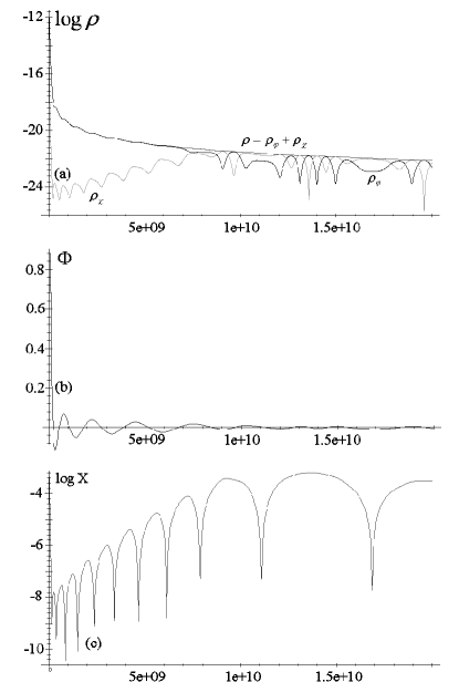
Figure 1: (a) Time evolution of $\rho_{\varphi}$, $\rho_{\chi}$ and $\rho$ during slow roll and first reheating, starting with $\rho_{\chi}{=}10^{{-}15}{\ll}\rho_{\varphi}{=}0.15{\cdot}10^{{-}11}$. Below: Evolution of the inflaton field $\Phi$ (b) and matter field $X$ (c) over the same time interval.

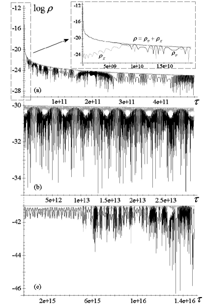
Figure 2: Time evolution of $\rho_{\varphi}$, $\rho_{\chi}$ and $\rho$ in different time intervals with different time scales, $\tau$ being reset to $0$ at the beginning of each: (a) before inflation, start with $\rho_{\chi}{=}10^{{-}15}{\ll}\rho_{\varphi}{=}0.15{\cdot}10^{{-}11}$ (the same as in Fig. 1), (b) much later, start with $\rho_{\chi}{=}10^{{-}30}{\gg}\rho_{\varphi}{=}10^{{-}34}$, (c) start with $\rho_{\chi}{=}\rho_{\varphi}{=}5{\cdot}10^{-41}$.

V Inflaton field model

The case of the parabola shaped potential (4) is essentially the scenario of Linde’s chaotic inflation linde . It is known that for the small value $\lambda\approx 10^{-14}$ an extreme inflationary expansion is obtained if the total density $\rho$ starts at about the Planck density linde . Therefore for numerical calculations a much lower initial value $\rho(0){\approx}0.16{\cdot}10^{{-}12}$ was chosen, leading to an inflationary enhancement of the scale factor $a$ by 35 orders of magnitude only. In order to obtain inflation, $p_{\varphi 0}=\dot{\varphi}^{2}_{\text{h}}/2-V_{\varphi}(\varphi_{\text{h}})<0$ must be satisfied which was achieved by setting $\dot{\varphi}_{\text{h}}(0)=0$ or $U(0)=0$. With this, according to Eqs. (40)

$$\Phi(0)=\left(\frac{4\rho_{\varphi}(0)}{\lambda}\right)^{1/4}\,.$$

For matter, between pressure and density a relation $\overline{p_{\chi 0}}=\gamma\overline{\rho_{\chi 0}}$ holds where $\gamma=1/3$ in the highly relativistic regime and $\gamma\ll 1/3$ in the non relativistic regime. With Eq. (30) for $m_{\chi}=0$ and $\overline{p_{\chi 0}}=\overline{y_{0}}/2-\alpha\varphi_{\text{h}}^{2}\overline{x_{0}}/2$ this relation leads to $\overline{y_{0}}=(1+\gamma)\alpha\varphi_{\text{h}}^{2}\overline{x_{0}}/(1-\gamma)$ and $\overline{x_{0}}=(1-\gamma)\overline{\rho_{\chi 0}}/(\alpha\varphi_{\text{h}}^{2})$ or, expressed in the variables introduced in Eqs. (33)–(34),

$$X = \frac{(1{-}\gamma)\rho_{\chi}}{\alpha\,\Phi^{2}}\,,$$ (42)

$$Z = \frac{1+\gamma}{1-\gamma}\alpha\Phi X\,.$$ (43)

These conditions were used as initial conditions for $X$ and $Z$. The exact value given initially to $\gamma$ turned out to be of no importance in the long run, so we used $\gamma=1/3$.

For $\rho_{\chi}$ various initial conditions were considered, from essentially no matter to equipartition between matter and inflaton field energy. The results are discussed in the following.

$\rho_{\chi}$ is first dramatically reduced by inflation (Fig. 1 and Fig. 2 (a), insert). When $\Phi$ starts to oscillate about $\Phi{=}0$, reheating sets in and $\rho_{\chi}$ is raised. The frequency of the heating oscillations is coupled to the one of the oscillations of $\Phi(t)$ and is approximately twice as large. The largest $\rho_{\chi}$ reached after reheating is a function of $\alpha$. The condition that $\rho_{\chi}=\rho_{\varphi}$ at some point in the evolution of the Universe yields the constraint $1.2\,\lambda\,{{}_{\textstyle<}\atop\textstyle\sim}\alpha{{}_{\textstyle<}\atop\textstyle\sim}3\,\lambda\,$. For the numerical calculations $\alpha{=}2\,\lambda$ was used. After $\rho_{\chi}$ and $\rho_{\varphi}$ coincide they start to oscillate in a chaotic manner around each other.

A phase portrait of $\varphi$ shown in Fig. 5 exhibits typical chaotic structure. Chaotic behavior arises naturally when two or more scalar fields interact with each other in an expanding Universe felder ; joras ; cornish , but it is usually of a transient type. The observed chaotic oscillations in the present model, on the contrary, are persistent. Even after quite large excursions $\rho_{\chi}(t)$ and $\rho_{\varphi}(t)$ always find back to each other. This kind of intermittent coincidence holds true for the whole decay of $\rho{=}\rho_{\chi}{+}\rho_{\varphi}$ from the very large values before inflation down to very small values like those of today.

It can qualitatively be understood as follows. From equations (35)–(37) and (40) one easily derives

$$\dot{\rho}_{\varphi}(\tau)=-6H\rho_{\varphi}+(3/2)\lambda H\Phi^{4}-\alpha X\Phi U$$ (44)

and

$$\frac{d(\rho_{\varphi}-\rho_{\chi})}{d\tau} = -6H(\rho_{\varphi}-\rho_{\chi})-3\alpha X\Phi^{2}$$ (45)

$$+\frac{3}{2}\lambda H\Phi^{4}-2\alpha X\Phi U\,.$$

The first term on the right hand side of Eq. (45) is always leading to a decrease of $\rho_{\varphi}-\rho_{\chi}$. The second term is $\leq 0$ and the third is $\geq 0$ so the two are counteracting, and numerically their sum turns out to be smaller than the first term. The last term is oscillatory and is dominant according to the numerical evaluation. It is a forcing term that leads to oscillations of $\rho_{\varphi}-\rho_{\chi}$ because according to Eqs. (37) and (44) one half of it increases $\rho_{\varphi}$ when the other half decreases $\rho_{\chi}$ and vice versa. A demonstration of this behavior is given in Figs. 3 which show results for $\rho_{\varphi}(\tau)-\rho_{\chi}(\tau)$ and $2\alpha X(\tau)\Phi(\tau)U(\tau)$.

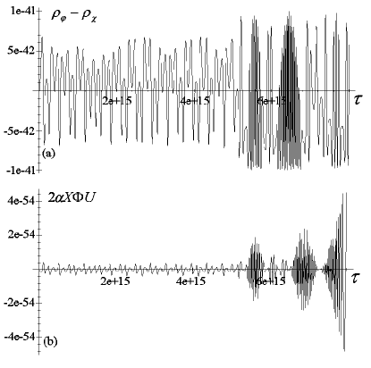
Figure 3: Density difference $\rho_{\varphi}(\tau)-\rho_{\chi}(\tau)$ and driving term $2\alpha X(\tau)\Phi(\tau)U(\tau)$ of equation (45). The same settings and initial conditions as in figure 2 (c) were used, but only about half of the time-interval was covered.

Some insight into the oscillations involved in the process is obtained by the following consideration. For $\chi_{\text{c}}=0$ combining Eqs. (35) and (36) yields

$$\ddot{\Phi}(\tau)=-3H\dot{\Phi}-\alpha X\Phi-\lambda\Phi^{3}\,.$$ (46)

This is an equation for the oscillations of $\Phi$ in which $-(\alpha X\Phi+\lambda\Phi^{3})$ is the driving force and $-3H\dot{\Phi}$ is a friction term. After a few oscillations through $\Phi=0$ the dominant term becomes $-\alpha X\Phi$, and from

$$\ddot{\Phi}(\tau)\approx-\alpha X\Phi$$

the oscillation frequency

$$\omega_{\Phi}\approx\sqrt{\alpha X}$$ (47)

is obtained. From Eqs. (38)–(39) we get

$$\ddot{X}(\tau)=-3H\dot{X}+4\rho_{\chi}-4\alpha X\Phi^{2}\,.$$

Again this is an equation for oscillations, this time of $X(\tau)$, with $-4\alpha X\phi^{2}$ being the driving term, and an approximate expression for the frequency of the oscillations is

$$\omega_{X}\approx 2\left|\Phi\right|\sqrt{\alpha}\,.$$ (48)

According to the numerical calculations, on the average

$$\frac{\omega_{X}}{\omega_{\Phi}}\approx\frac{2\left|\Phi\right|}{\sqrt{X}}$$

is smaller than 1 whence the oscillations of $X$ are slower than those of $\Phi$. In consequence, in the short run the frequency $\omega_{\Phi}\approx\sqrt{\alpha\chi}$ of the $\Phi$ oscillations varies between smaller and larger values as can be clearly seen in Figure 4 and is also reflected in Fig. 3. In the long run $X$ decreases like all other variables of the system of Eqs. (35)–(40). Therefore, as time goes on, the average frequency of the $\Phi$ oscillations and through this also that of the oscillations of $\rho_{\varphi}$ and $\rho_{\chi}$ around each other is slowly decreasing.

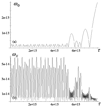
Figure 4: Approximate frequencies $\omega_{\Phi}\approx\sqrt{\alpha X}$ and $\omega_{X}\approx 2\left|\Phi\right|\sqrt{\alpha}$, for the same settings and initial conditions as used in figure 2 (c), but only about half of the time-interval was covered.

Obviously the chaotic nature of the system is still quite structured, because roughly the two frequencies $\omega_{X}$ and $\omega_{\Phi}$ remain visible as organizing factors. It is well known that in linear systems with two incommensurable frequencies ergodic phase portraits are obtained. It appears that the chaoticity of the present system is caused by a permanent change of the ratio $\omega_{\Phi}/\omega_{X}$. In this process, due to the overwhelming abundance of irrational numbers, the change between different measures of incommensurability leads to a certain amount of unpredictability.

Because it was not possible to calculate the full evolution from inflation to the present state, the time-averaged coincidence of $\rho_{\varphi}$ and $\rho_{\chi}$ claimed above was tested piecewise in more than ten different $\rho$-regimes from very large to very small, starting with many different values of the ratio $\rho_{\chi}/\rho_{\varphi}$ in each. Fig. 2 shows 3 typical examples.

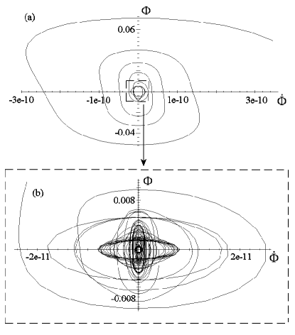
Figure 5: Phase portraits of the inflaton-field $\Phi$: (a) the same time interval and same initial settings as in Fig. 1 were used, only the slow roll phase is omitted; (b) continues where (a) stopped and covers the rest of the time interval used in Fig. 2 (a) – the chaotic nature of the oscillations is easy to see.

For the evolution of $\varrho$ after inflation the approximate validity of $\varrho a^{\nu}{=}\text{const}$ was found with $\nu{\approx}4$ in (a), $\nu{\approx}3.9$ in (b) and $\nu{\approx}4$ in (c) etc., i.e. the usual relativistic equation of state, $\varrho a^{4}{=}\text{const}$, is a good approximation to the evolution of the (rather smooth) total density $\varrho$.

VI Remarks on the Coincidence Problem

In Ref. dodelson an idea for a solution of the coincidence problem caldwell was elaborated: The inflaton field energy, called dark energy there, has periodically dominated in the past, giving a finite probability to its observed preponderance today. The oscillations are achieved by sinusoidal modulations of an exponentially decaying potential for the scalar field representing dark energy, i.e. by the assumption of a periodic forcing.

Our model leads to a similar behavior, only that the oscillations are not purely periodic but slightly chaotic. In contrast to Ref. dodelson they are not implied by an imposed forcing but caused by the oscillations of the inflaton field $\Phi$ around $\Phi=0$ and its interaction with the matter field $\chi$. The mechanism is the following: The oscillations of $\Phi(t)$ cause heating oscillations by which again and again the energy density of matter is temporarily raised above the energy density of the inflaton field. Since with decreasing amplitude of the $\Phi$ oscillations also the frequency is getting smaller and smaller, the periods with a preponderance of either matter or inflaton field become increasingly longer.

In our model the alternating preponderance of matter and inflaton field was observed over a density range from $10^{-12}$ to $10^{-115}$ with the same set of parameters $\alpha$ and $\lambda$. However, in spite of its continuous increase at low densities the average period of preponderance is still too small by orders of magnitude. With $\lambda=10^{-120}$ instead of $\lambda=10^{-14}$ a reasonable period (small fraction of the life time of the universe) can be achieved, but with this small value the behavior at large densities is no longer the needed reheating scenario, which was found only down to values $\lambda{{}_{\textstyle>}\atop\textstyle\sim}10^{-40}$. At first glance it would appear that a potential $V(\Phi)$ that decays like $10^{-14}\Phi^{4}$ at large $\Phi$ and like $10^{-120}\Phi^{4}$ at small $\Phi$ would lead to a solution. It turns out, however, that an effective reheating at large densities requires a large value of $\lambda$ even around $\Phi=0$.

At second glance a dynamic $\lambda=\lambda(t)$ would appear to do it, and $\lambda(t)\sim H^{2}(t)$ would look like a good choice, coupling the potential directly to the energy of the gravitational field. However, in a reasonable dynamical evolution pressure and density should be connected by $\overline{p_{\chi 0}}=\gamma\overline{\rho_{\chi 0}}$ and in consequence, Eq. (42) should hold. From this and (47) we get

$$\omega_{\Phi}\approx\frac{\sqrt{\rho_{\chi}}}{|\Phi|}\approx\frac{H}{|\Phi|}\geq\frac{H}{\mbox{max}\,|\Phi|}.$$

While at later times $\omega_{\Phi}\approx H$ would have the desired order of magnitude because $1/H$ is approximately the age of the universe, the small factor $1/\left|\Phi\right|$ spoils any attempt to obtain reasonably small frequencies.

From our studies it can be concluded, that the oscillations of the inflaton field and its interaction with matter can keep the energy densities of the two close together over the full range of densities from inflation to present day densities, with alternating preponderance of one of the two. Reasonable times for the duration of the preponderance at present day densities cannot be obtained from our model. So oscillations of the inflaton field and periodic reheating of matter through a coupling between matter and inflaton field may be one clue to the solution of the coincidence problem but cannot provide a full solution of it. The simple model for describing matter adopted in this paper is certainly not appropriate for later stages in the evolution of the universe, and a better adapted model might improve the situation.

VII Higgs field model

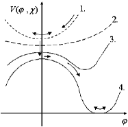
Figure 6: Potential (3) for 4 different values of $\overline{x_{0}}\chi$ that decrease in the shape sequence 1,2,3,4. During pre-inflation shapes 1 and 2 are active, during inflation shape 3. 4 is the final shape when matter is already very diluted.

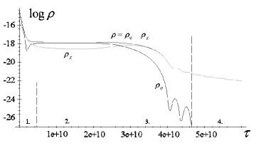
Figure 7: Time evolution of $\rho_{\varphi}$ and $\rho_{\chi}$ for the potential (3) that evolves according to Fig. 2.

For the potential (3) calculations were done with $V_{0}{=}1.25{\cdot}10^{-18}$, $\lambda{=}2{\cdot}10^{{-}17}$, $\alpha{=}\lambda/10$, $\chi_{c}{=}\sqrt{5}$, $m_{\chi}^{2}{=}1{\cdot}10^{{-}19}$ and with the initial values $\rho_{\chi}{=}7.5{\cdot}10^{{-}16}$, $\rho_{\varphi}{=}3{\cdot}10^{{-}15}$ of the densities. First the potential assumes shape 1 of Fig. 6, and $\varphi$ starts at a value for which $V$ is well above its minimum at $V{=}0$. As $\varphi$ rolls slowly towards this, $\rho_{\chi}$ decreases whence $V$ gradually assumes a flatter shape like 2. When $\varphi$ reaches the region around $\varphi{=}0$, $\rho_{\chi}$ may be enhanced through oscillations of $\varphi$ in the potential well but is then again diluted by ongoing inflation. Finally $\overline{x_{0}}{=}\overline{\tilde{\chi}^{2}}$ becomes smaller than $\chi_{c}^{2}$ and $V(\varphi)$ assumes a sombrero-like shape as 3. Then $\varphi$ starts to roll downhill towards a new minimum appearing at a $\varphi{\neq}0$. Oscillations around this lead to an increase of $\rho_{\chi}$. Due to the change of shape of the potential the oscillation frequency changes and thus parametric resonance occurs at many different frequencies, leading to an especially effective reheating. Asymptotically, shape 4 will be assumed and $\varphi$ will settle at the minimum $V{=}0$ obtained from Eq. (3) for $\chi{=}0$. The dynamics can be separated into four qualitatively different steps (Fig. 7). 1. Pre-inflation: Slow roll in a potential of shape 1-2 towards $\varphi{=}0$ with possible reheating through oscillations around $\varphi{=}0$. 2. Inflation: Slow roll from $\varphi{=}0$ in a potential of shape 3 towards a new minimum at $\varphi{\neq}0$. 3. Reheating: Oscillations around the new minimum. 4. Friedmann-like evolution after the settlement of $\varphi$ at the new minimum. These four steps are found for a wide variety of parameters and initial conditions.

A model combining the properties of the two cases considered, chaotic oscillations with alternating dominance of matter and inflaton field as well as dynamic symmetry breaking, should be obtainable by employing two inflaton fields of type $\varphi=\varphi_{\text{h}}(t)+\varepsilon\tilde{\varphi}(\vec{x},t)$, one moving in a parabola- and the other in a sombrero-like potential, and both being coupled to the matter field.

VIII Conclusions

The main result of this paper consists in a set of equations for the interaction between a scalar inflaton field, a scalar matter field and the gravitational field, obtained by averaging processes. Due to the averaging no specific assumptions about the inhomogeneities of the matter field like specifying any initial conditions must be made. The set of equations can be applied to pre-inflation, inflation and the reheating after inflation. It contains the heating effects of parametric resonance and is nevertheless rather easy to handle. However, it should be noted that the presented approach is neither covariant, nor gauge invariant. Therefore one has to take great care to compute only physically meaningful quantities, as in the studied cases.

Processes like the dynamic symmetry breaking of a Higgs field, the theoretical description of which usually requires quite some effort, are easily obtained and understood. An attempt to gain some insight into the coincidence problem was made. Repeated periods of matter reheating can keep the energy densities of the inflaton and the matter field close together for all times until today and lead to an alternating dominance of one of them. The preponderance of the inflaton field observed today would thus be a question of chance and be preceded by a preponderance of matter. However, the specific model employed for describing this process did not yield reasonable durations of preponderance over the full evolution from inflation until today. We therefore conclude that it may provide one clue to the understanding of the problem while other clues may still be missing.

Acknowledgment. This work was partly supported by Deutsche Forschungsgemeinschaft. E. R. expresses his gratitude for hospitality and support of the Physics Dept. at Brown University, Providence, R. I., USA, received in the initial phase of this work. Valuable discussions with R. Brandenberger are gratefully acknowledged.

IX Appendix

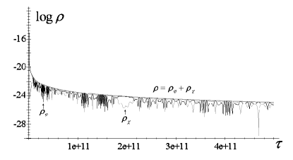
Figure 8: Time evolution of $\rho_{\varphi}$, $\rho_{\chi}$ and $\rho$ computed to order $n=1$. The same time interval and initial conditions as in Fig. 2 (a) were used, except for $a$ and $\overline{x_{1}}$ which was set to $a_{i}\equiv m_{\text{P}}^{-1}$ and $\overline{y_{0}}a_{i}^{2}/10$ respectively. Comparison with Fig.2 (a) shows a similar evolution of the densities.

The quality of the approximation provided by equations (35)–(40) can easily be tested by truncation to higher orders. Truncating to order $n=1$ enhances our set (35)–(40) by two equations and the two variables $x_{1}$ and $y_{1}$ as

$$\ddot{\overline{x_{0}}} = 2\overline{y_{0}}-2\overline{x_{1}}/a^{2}-3H\dot{\overline{x_{0}}}-2(\alpha\varphi_{\text{h}}^{2}+m_{\chi}^{2})\overline{x_{0}}\,,$$

$$\dot{\overline{y_{0}}} = -6H\overline{y_{0}}-\dot{\overline{x_{1}}}/a^{2}-(\alpha\varphi_{\text{h}}^{2}+m_{\chi}^{2})\dot{\overline{x_{0}}}\,;$$

$$\ddot{\overline{x_{1}}} = 2\overline{y_{1}}-3H\dot{\overline{x_{1}}}-2(\alpha\varphi_{\text{h}}^{2}+m_{\chi}^{2})\overline{x_{1}}\,,$$

$$\dot{\overline{y_{1}}} = -6H\overline{y_{1}}-(\alpha\varphi_{\text{h}}^{2}+m_{\chi}^{2})\dot{\overline{x_{1}}}\,.$$

In addition, one needs to compute the time evolution of the scale factor $a$ by means of equation (32) simultaneously, since it enters the equations now.

In view of their chaotic character a detailed comparison of the fine structure of the solutions obtained with truncation to order $n=0$ and to order $n=1$ is not meaningful. However, the average behavior in the long run must be comparable, and indeed all computations yielded the same qualitative and essentially the same quantitative behavior - compare Fig. 2 (a) with Fig. 8 as an example. No crucial dependence on the initial values of $\overline{x_{1}}$ and $\overline{y_{1}}$ was observed, so we choose $\overline{x_{0}}=(1-\gamma)\rho_{\chi}/(\alpha\Phi^{2})$, $\overline{y_{0}}=(1+\gamma)\rho_{\chi}/2$,$\overline{x_{1}}=(1+\gamma)\rho_{\chi}/2$ and $\overline{y_{1}}=0$, with $\gamma=1/3$ in Fig. 8. As an initial value for the scale factor we choose $a=m_{\text{P}}^{-1}$, corresponding to a Planck sized patch of the Universe.

By the same token the Higgs field model of section VII was checked up to second order and no essential difference of the long run behavior was found either.

From this comparison it can be concluded that truncation to the order $n=0$ already provides a very good approximation.

References

- (1) A. Linde, Particle Physics and Inflationary Cosmology (Harwood, Chur, Switzerland, 1990).
- (2) D. H. Lyth and A. Riotto, Phys. Rep. 314, 1 (1999).
- (3) R. Brandenberger, in Large Scale Structure Formation edited by R. Mansouri and R. Brandenberger (Kluwer, Dordrecht, 2000).
- (4) L. Kofman, A. Linde, and A. Starobinsky, Phys. Rev. D 56, 3258 (1997).
- (5) P. Greene, L. Kofman, A. Linde, and A. Starobinsky, Phys. Rev. D 56, 6175 (1997).
- (6) L. Kofman, A. Linde, and A.Starobinsky, Phys. Rev. Lett. 73, 3195 (1994).
- (7) J. Traschen and R. Brandenberger, Phys. Rev. D 42, 2491 (1990).
- (8) Y. Shtanov, J. Traschen and R. Brandenberger, Phys. Rev. D 51, 5438 (1995).
- (9) S.E.Jorás, V.H.Cárdenas, Phys. Rev. D 67, 043501 (2003).
- (10) G. Felder and L. Kofman, Phys. Rev. D63 103503 (2001).
- (11) A. L. Liddle and D. H. Lyth, Cosmological inflation and Large-Scale Structure, (Cambridge Univ. Press, Cambridge 2000)
- (12) A. K. Raychaudhuri, Phys. Rev. 98, 1123 (1955)
- (13) A. K. Raychaudhuri, Theoretical Cosmology, (Clarendon, Oxford, 1979)
- (14) R. Balescu, Transport Processes in Plasmas, (Elsevier, Amsterdam, 1988)
- (15) N.J. Cornish and J.J. Levin, Phys. Rev. D 58,3022 (1996).
- (16) S. Dodelson, M. Kaplinghat and E. Stewart, Phys. Rev. Lett. 85, 5276 (2000)
- (17) R. Caldwell, R. Dave and P.J. Steinhardt, Phys. Rev. Lett. 80, 1582 (1998)