[
On the Initial Conditions for Brane Inflation
Abstract
String theory gives rise to various mechanisms to generate primordial inflation, of which “brane inflation” is one of the most widely considered. In this scenario, inflation takes place while two branes are approaching each other, and the modulus field representing the separation between the branes plays the role of the inflaton field. We study the phase space of initial conditions which can lead to a sufficiently long period of cosmological inflation, and find that taking into account the possibility of nonvanishing initial momentum can significantly change the degree of fine tuning of the required initial conditions.
pacs:
PACS numbers: 98.80Cq]
I Introduction
The paradigm of cosmological inflation [1] has been spectacularly successful as a theory of the very early Universe. Not only does having a very early period of cosmological inflation solve some of the mysteries of Standard Big Bang cosmology such as the horizon and the flatness problems, but it also gives rise to a mechanism which generates the primordial fluctuations required to explain today’s cosmological large-scale structure and the observed anisotropies in the cosmic microwave background (CMB). Simple models of inflation rather generically predict a scale-invariant spectrum of adiabatic cosmological fluctuations, a prediction which has recently been verified with significant accuracy by CMB anisotropy experiments [2, 3, 4, 5, 6].
However, at the present time the paradigm of cosmological inflation is lacking an underlying theory. The inflaton, the scalar field which is postulated to generate the quasi-exponential expansion of the Universe, cannot be part of the standard particle physics model, nor does it fit easily into pure field theory extensions of the standard model (see e.g. [7] for a recent review of progress and problems in inflationary cosmology). In particular, it is not easy to justify a pure field theory based model of inflation in which the potential of the inflaton is sufficiently flat in order not to produce too large an amplitude of the fluctuation spectrum. Moreover, in many simple scalar field toy models of inflation, the overall amplitude of the spectrum of fluctuations points to a scale of inflation which is close to the scale of particle physics unification, and thus close to the scale where new fundamental physics, e.g. string theory, will become important. Thus, it is natural to look for realizations of inflation in the context of string theory.
One of the key observations which makes it promising to consider string theory as the source of cosmological inflation is the fact that string theory contains many scalar fields (the moduli fields) which are massless in the absence of non-perturbative effects and in the absence of supersymmetry breaking. Hence, it is natural to look for ways of obtaining inflation from moduli fields. Recent developments in string theory have led to new possibilities. In particular, based on the observation that string theory contains p-branes as fundamental degrees of freedom, and that the matter fields of the Universe can be considered to be localized on these branes, the brane world scenario has emerged in the past few years offering a complete change in our view of the Universe [8].
Within the context of brane world scenarios, there are new ways to obtain inflation. For example, if the brane which represents the space-time on which our matter fields are confined is moving in a nontrivial bulk space-time, it is possible to obtain inflation on the brane from the dynamics in the bulk (“mirage inflation” [9, 10, 11]). Another possibility is topological inflation on the brane [12]. The approach which was first suggested in [13] and has received most attention in the literature is “brane inflation”, a scenario in which inflation on the brane is generated while two branes are approaching each other. In this scenario, the separation of the branes plays the role of the inflaton.
The basic idea of brane inflation is the following [13]: consider two parallel BPS branes (see e.g. [14] for the string theory background). When they sit on top of each other the vacuum energy cancels out. In the cosmological setting, they will start out relatively displaced in the extra dimensions. There is then an attractive force between the branes due to exchange of closed string modes, the stringy realization of the gravitational attraction between the branes. If supersymmetry is unbroken, the gravitational attraction is cancelled out by the repulsion due to the Ramond-Ramond (RR) field. The separation between the two branes acts as a scalar field in the effective field theory on the brane. With two parallel BPS branes, the potential for this scalar field is flat before supersymmetry breaking, and hence no cosmological inflation can be induced. After supersymmetry breaking, only the graviton remains massless, and hence there will be a net gravitional attractive force between the branes. The induced nonperturbative potential is flat and hence can yield a period of cosmological inflation on the brane while the branes are widely separated.
Following the pioneering work of [13], several concrete realizations of the basic scenario were proposed which have the advantage of allowing for controlled computations of the inter-brane potential (see [15] for a recent review). One realization [16, 17] which will be analyzed in Section 3 is based on a D4 brane-antibrane pair in Type IIA string theory compactified on an internal torus . The brane pair is parallel but separated in internal space. In this case, the potential can be computed explicitly. It turns out that a sufficient period of inflation can be obtained provided the branes are located approximately at the antipodal points. This leads to a severe initial condition constraint on the model. By fixing the branes to orientifold fixed planes [18] this initial condition constraint can be somewhat alleviated. Another brane inflation scenario [19, 20, 21, 22] is based on taking two D4 branes which again are parallel except for forming an angle (taken to be small) in one of the two-dimensional hyperplanes. In this case, the attractive potential is once again computable in string perturbation theory, and the resulting potential is suppressed by the small parameter , thus making the probability to obtain sufficient inflation larger. The brane inflation paradigm appears in fact to be rather robust. Models based on the attractive force between branes of different worldsheet dimensionalities were considered in [23, 24, 25, 26].
A question which has not yet been addressed in the literature on brane inflation is the issue of constraints on the phase space of initial conditions for inflation which arise when one takes into account the fact that in the context of cosmology the momenta of the moduli fields which give inflation cannot be neglected in the early Universe. For simple scalar field toy models of inflation, the constraints on the phase space of initial conditions taking into account the range of allowed initial values not only for the inflaton field, but also for its momentum, were studied in [27, 28, 29, 30, 31, 32, 33]. As this work showed, there is a big difference in the degree of tuning required in order to obtain sufficient inflation between small-field inflation models of the type of new inflation [34, 35] and large-field inflation models such as chaotic inflation [36] ***See [37] for the classification of inflationary models into those of small-field and large-field type..
For models of the type of new inflation, the work of [28, 29] showed that allowing for nonvanishing intial field momenta may dramatically reduce the phase space of initial conditions for which successful inflation results. This result is easy to understand: in new inflation, the field must start off close to an unstable fixed point, from which point it then slowly rolls to its minimum. Unless the initial field momentum is finely tuned (as finely or even more finely that the field value), slow rolling is never realized. In contrast, in models of the type of chaotic inflation, most of the energetically accessible field value space gives rise to a sufficiently long period of slow roll inflation. Since the momentum redshifts much faster than the potential energy, the initial kinetic energy does not have to be small in order that the field will settle down close to the slow-roll trajectory (see also [38] for a recent extensive phase space study of homogeneous inflationary cosmology) †††Note that the studies of [28, 29, 38] mentioned above were performed without taking inhomogeneities into account. As studied in [32] for new inflation and in [30, 31, 32, 33] for chaotic inflation, including spatial inhomogeneities accentuates the difference between models like new inflation and those like chaotic inflation. Inhomogeneities further reduce the measure of initial conditions yielding new inflation, whereas the inhomogeneities have sufficient time to redshift in chaotic inflation, letting the zero mode of the field eventually drive successful inflation. The property of chaotic inflation as an attractor in initial conditon space [31] persists even when including linearized gravitational fluctuations [39]. Note that natural inflation models [40] fall into the former category (and thus are not natural at all from the dynamical systems perspective), whereas hybrid inflation [41] models are more like chaotic inflation in terms of the initial condition aspect.
In the following section, we review the constraints on the initial conditons in phase space required for successful inflation and formulate the argument in a form which is applicable to general models of inflation driven by a single scalar field. This then allows us to apply (in Section 3) the arguments to a couple of representative models of brane inflation. We find that in some models of brane inflation, in particular in the case of branes at an angle, there is dramatic reduction to the relative probability of obtaining successful inflation when allowing the initial momentum to be general when compared to what it obtained allowing only the initial field position to vary and taking the initial momentum to vanish. In these models, the sensitivity of brane inflation to initial conditions is worse than in the case of chaotic inflation.
II Method
There have been a large number of inflationary models proposed over the years. These models can be divided into two classes, large field (e.g. chaotic inflation) and small field inflation (e.g. new inflation). In all these models slow roll inflation must last long enough to solve the flatness, horizon, and monopole problems. This requires [1] that the Universe inflate during slow roll by at least e-foldings. In the following, we develop a general method for determining the constraints on the phase space of initial data resulting from enforcing these requirements. Specifically, we want to consider the allowed values for the initial kinetic term that will still allow for adequate inflation.
We will first give some general considerations applicable to both classes of inflationary models, and only later consider separately the cases of small field and large field models. We will find that in the latter case one can achieve adequate inflation quite naturally, while the former suffers from fine-tuning of initial conditions if one wants successful inflation and considers the full energetically allowed phase space of initial conditions for both the inflaton field and its momentum.
We will restrict our attention to homogeneous evolution of the inflaton field. Small inhomogeneities could be included using the methods of [39].
A General Phase Space Considerations
We want to find which regions of the phase space will lead to successful inflation (here, is the inflaton field and is its velocity). From the point of view of early Universe cosmology it is unreasonable to postulate that starts at some distinguished value (as was initially assumed in models of new inflation), nor is it justified to set the initial momentum to zero. The full phase space of initial conditions depends on the specific inflationary model being considered. For example, in models in which inflation is to commence immediately after the Planck time, a reasonable condition is to bound the phase space by requiring that the total energy density be smaller than the Planck density. Given initial conditions anywhere in this allowed phase space, we ask what subset of these initial conditions will lead to trajectories with a sufficiently long period of slow roll inflation (inflation not necessarily starting immediately at the initial time).
The slow roll conditions for inflationary dynamics single out a special trajectory in phase space. In order to have successful slow roll inflation, the phase space trajectory of the inflaton field must, during some time interval, be sufficiently close to the portion of the trajectory which yields a sufficient number of e-foldings of inflation in order to solve the cosmological problems mentioned at the beginning of this section. Our method (motivated by the work of [28, 29]) is to follow these trajectories backwards in time to uncover the entire phase space that leads to successful inflation.
Let us begin by recalling the relevant equations of motion, which are the field equation for the inflaton and the Friedmann equation,
| (1) |
| (2) |
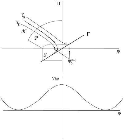
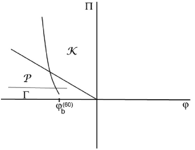
Given these equations we proceed by dividing the phase space into regions , , and as indicated in Figures 1 and 2. The region is the region where the potential energy dominates over the kinetic energy, but the slow roll conditions (even in the generalized sense discussed below) are not satisfied, and the is the region of phase space where the kinetic energy dominates.
Region is the region of generalized slow roll. To define this region, let us remind the reader that the usual slow roll conditions of inflationary dynamics state that we can neglect the kinetic energy compared to the potential in (2) and compared to in (1). Under these assumptions, the equations become
| (3) |
| (4) |
The solution to these equations is a curve in phase space. As has recently been studied in detail in [38], in an expanding Universe, this curve is an attractor curve. The curve does not extend to all values of , since the slow roll conditions break down.
There is a region of phase space which forms a very narrow strip about the curve and which extends from the curve to the axis and slightly beyond, where the potential energy density dominates over the kinetic energy density, but where in the scalar field equation of motion neither the nor the terms are negligible (see Figure 1). A phase space trajectory must enter region if slow roll inflation is to occur at all.
Along the curve there is a distinguished value of which we will denote as . If the “beginning” value of obeys
| (5) |
then the trajectory will experience a sufficient number of e-foldings of inflation. By integrating the slow roll equations (3,4), we find that is given by
| (6) |
where is the value of the field where the slow roll approximation breaks down. For the case of small field inflation ‡‡‡Without loss of generality we may assume for small field inflation that is the local maximum of the potential near which inflation occurs, and for simplicity we take the potential to be symmetric about . In the case of large field inflation, we take to be the minimum of the potential, and again we take the potential to be symmetric about this field value. the constraint (5) is given by and gives the constraint for large field models (see Figure 2).
From the region we trace the evolution backwards to the region . In this region the potential still dominates the kinetic term, but instead of the term, it is the term in the scalar field equation of motion which is negligible. Thus, in this region (1) and (2) become,
| (7) |
| (8) |
Equations (7) and (8) for a general form of the potential can be combined into one equation,
| (9) |
where and are the values at the boundary between regions and . If we assume that is almost constant in region the above relation simplifies to a linear relation between and in this region,
| (10) |
The consistency of this approximation must be investigated for each potential separately. The condition for the approximation to be good can be written as (within a first order analysis):
| (11) |
As will be discussed later, this condition is not satisfied for all models of inflation.
Let us now denote by and the values of the inflaton and its momentum when the trajectory enters the generalized slow roll region . These values are related to and via (10), and thus
| (12) |
where we have neglected since it is much smaller than .
The boundary between regions and is given by the equality of kinetic and potential energy
| (13) |
The sign in the above equation depends on whether one is in the region of increasing or decreasing . For concreteness, we will consider trajectories with . Substituting from above equation into (12) and keeping in mind the approximation of V being constant will lead to:
| (14) |
Solving (10) for we can also write the equation for the trajectories in phase space while they are in ,
| (15) |
We now want to extend the trajectories back further to determine which of the trajectories which begin in region will lead to successful inflation, where is the region of kinetic energy domination, i.e. . Here we are interested in trajectories that will loose enough kinetic energy (due to the Hubble friction) to eventually reach region . In region we can ignore the effects of the potential and (1) and (2) become:
| (16) | |||
| (17) |
These can be integrated and we find:
| (18) |
where - as used earlier - and are the values at the boundary between regions and . These regions meet along the curve . We can solve (18) for to find the equation for trajectories in :
| (19) |
These trajectories continue all the way until breaks down or they reach the boundary of phase space as given by the particular theory (e.g. Planck energy density in the case of chaotic inflation, or the limiting value of if the inflaton corresponds to the separation of two branes in an extra dimension and the radius of this extra-dimensional space is bounded).
Now that we have developed the necessary equations to describe the full phase space, let us consider the cases of small and large field inflation separately.
B Small Field Inflation
Let us first focus on the case of small field inflation models such as new inflation. An example of a potential which leads to small field inflation is sketched in Figure 1 (lower panel). In this case, during the period of slow roll inflation is close to .
We want to calculate the whole volume of phase space that leads to successful slow roll inflation. Most of this phase space consists of points in and whose trajectories enter the region . In particular, to obtain enough e-foldings of slow roll inflation, the value of for such a trajectory must obey
| (20) |
Our method will be to follow the two limiting phase space trajectories (those for which the inequality in (20) is saturated and which are labelled and in Figure 1) back into regions and and then to add up the corresponding phase space volumes between the two curves in both regions. Note that since the volume of is negligible in comparison to the volume of (in particular, the value of is negligible in region compared to ), we can neglect the contribution of the small subset of phase space within that leads to enough e-folding of inflaton.
The calculation involves extending the trajectories through the region by making use of (15). Making use of (14) and assuming that the condition (11) is not violated, we obtain the following range of values of which lead to trajectories with successful slow roll inflation:
| (21) |
From this result, it is obvious that our approximation of assuming that the condition (11) applies throughout region is not satisfied in many examples motivated by conventional quantum field theory in four dimensional space-time, since in those models we could expect the minimum of the potential to be at a value of smaller than the value of resulting from (21).
According to Equation (15), trajectories in are parallel straight lines with a negative slope which extend all the way to , and the above equation determines the side borders for trajectories leading to successful slow roll inflation.
Combining these results, we find that the volume of phase space contained in region leading to successful slow roll inflation is
| (22) | |||||
| (23) |
For a general potential for which the condition (11) is not satisfied throughout, we have to find the equations of the trajectories using equation (9), and use the results to obtain the phase space points and which form the end points of the boundary between and in the subspace of phase space leading to successful slow roll trajectories. Here, the superscripts and stand for the lower and the upper boundary trajectories, respectively. In this case, the volume is:
| (24) |
Finally, we must determine the phase space volume within region bounded by the two trajectories and , trajectories which in region obey the equation (19). However, this time there arises the crucial issue of how far back to integrate the trajectory. First, for the classical field theory analysis to be valid, the energy density cannot exceed the Planck density, and this imposes an upper limit on the allowed value of , namely
| (25) |
Next, the domain of may be bounded according to the physics which determines what the inflaton is. For example, if the inflaton corresponds to the separation between two branes in a transverse compact dimension, then is bounded by the radius of the compact dimension. Finally, in the case of potentials which rise again as , the condition, will cease to hold at sufficiently large values of §§§The region of phase space beyond this bound would again be an inflating region, but not one corresponding to small field inflation..
If there is a cutoff of the type described above, we will denote the cutoff values of the phase space coordinates by and .
We obtain the part of the phase space volume contained within corresponding to successful slow roll inflation by integrating the trajectories and through region using Equation (19) from to , and computing the phase space volume between the curves:
| (26) |
where and are given by (19) evaluated at
| (27) |
Note that there is an equal size region in phase space obtained by reflection about the origin of phase space.
Since is very small compared to both and to the typical energy scale in the potential, we can first of all replace the lower integration limit in both integrals in (26) by the average of the two lower limits, which is . Next, we can Taylor expand the difference between and (making use of (19)) about the value of obtained from the value of along the central of the three diagonal curves in the upper left quadrant of Figure 1, with the result
| (28) | |||||
| (29) |
where we have made use of (13) to replace the factor appearing in (19) by the term involving the potential.
Making use of this approximation, it is easy to evaluate equation (26) and find :
| (30) |
Recall that is negative due to the assumption (27) on which half of phase space we are considering. Note also that the second term in the square brackets in (30) cancels with the positive contribution of , thus yielding
| (31) |
Note that in the above, we have assumed that the approximation (11) is valid in the entire region . For typical symmetric double well potentials with minima at , this is only satisfied for values of larger than ¶¶¶If the condition (11) is not satisfied, our result yields an upper bound on the phase space of successful slow roll inflation.. For inflationary models in the context of grand unified field theories, this is not a realistic assumption, however in the cases of brane inflation considered in the following section, the assumption more likely to be justified (as long as the brane inflation model does not involve a hierarchy of scales of internal dimensions).
Let us consider two concrete examples. In the first example we assume that the potential keeps decreasing (towards the value zero) at large values of , and that there is a cutoff on the range of values of at ∥∥∥It is easy to check that in this example the trajectories stay below the cutoff line (25) if the value of the potential at the origin is several orders of magnitude lower compared to the Planck density, as it must if inflation is not to generate a too large amplitude of gravitational waves. In this case, we obtain
| (32) |
The total allowed phase space volume is
| (33) |
and hence the fraction of the phase space volume which leads to successful slow roll inflation is
| (34) |
where is the contant appearing in the exponential in (32).
If we compare the result (34) with what would be obtained by considering only the configuration space constraint on the initial conditions for successful slow roll inflation, we find that the constraint is more severe by a factor which is given by the second ratio on the right hand side of (34).
In the second example, we consider a model of the type proposed in new inflation, with a potential of Coleman-Weinberg [42] type
| (35) |
with chosen such that (11) is satisfied in the entire region . This potential rises at large values of , and thus the cutoff value is determined either by the potential energy becoming equal again to the kinetic energy, i.e.
| (36) |
or by the kinetic energy density reaching the boundary (25), which will occur at the value determined by
| (37) |
For small values of the potential at the origin, it is the condition (37) which determines the largest value of . Inserting the result into (31), we otain
| (38) |
The total phase space is determined by (25) and by the largest value of for which :
| (39) |
Hence, the fraction of phase space which leads to successful slow roll inflation is given by
| (40) |
which is the same order of magnitude as the fraction of configuration space which leads to successful slow roll inflation. Thus, in this example including nonvanishing initial momentum does not lead to a reduction in the relative phase space of initial conditions yielding slow roll inflation compared to the fraction of configuration space yielding slow roll inflation assuming vanishing initial momenta. The reason is that for any initial field value, we can choose a finely tuned initial momentum for which the field will roll up the potential and land near the origin with vanishing momentum.
C Large Field Inflation
The fraction of the energetically allowed phase space of initial conditions which leads to successful slow roll inflation is of order one in most large field inflation models. This is not hard to understand: First of all, the volume of configuration space which is energetically allowed and also gives sufficient inflation is of order unity. Second, the phase space trajectories approach the slow rolling curve sufficiently fast such that taking the freedom in the choice of the initial momentum into account does not lead to any restriction on the allowed phase space which gives slow roll inflation.
To be specific, let us consider the chaotic inflation model given by the potential
| (41) |
where the constraints on the amplitude of the fluctuations spectrum limits the mass to be .
In this example, the slow roll trajectory is given by
| (42) |
The boundary between regions and is given by
| (43) |
and thus the slow roll trajectory ends at the value
| (44) |
The value ( required in order to have sufficient slow roll inflation) is slightly larger than the above value, about .
In this example, we can solve for the trajectories in Region without making the assumption that the potential is approximately constant. The result is
| (45) |
To get a lower bound on the phase space of initial conditions which yield sufficient slow roll inflation we will extend the above trajectories (45) beyond the boundary between and . Taking to be negligible compared to and neglecting compared to , we find that the trajectories (45) hit the phase space boundary at the value given by
| (46) |
Thus, a lower bound on the allowed phase space of initial conditions which give sufficient slow roll inflation is obtained by considering the volume of phase space with and arbitrary . Thus, the fraction of phase space yielding successful slow roll inflation is bounded by
| (47) |
where is the value of for which the potential energy reaches Planck density.
III Application to Brane Inflation
In this section we will apply the methods developed in section two to some current models of brane inflation. Many models of brane inflation have been proposed over the years [13, 16, 17, 18, 20, 21, 22, 23, 24, 25]. Let us briefly review the common features of these models (a more detailed review can be found in [15] and references within). The starting point is a stack or at least a pair of parallel p-branes. The p-branes are taken to be large in three spatial dimensions and the remaining dimensions of the brane are wrapped on the compactified parallel volume, . The branes are separated by a distance in the remaining transverse dimensions which are also taken to be compact with volume . The branes appear as BPS states protected by supersymmetry (SUSY) and are parallel, static, and stable. This is realized through the potential for the branes, which vanishes because the forces from the Neveu-Schwarz (NS) sector, which contains the dilaton and graviton, are exactly canceled by the forces due to the Ramond-Ramond (RR) charge. The idea behind brane inflation is to break the SUSY to generate a flat, attractive potential between the branes. Once a nonzero potential is generated, the inflaton is identified with the separation of the branes in the transverse volume . For large the potential has a form expected from Newtonian gravity, which can be understood since the dilaton and graviton are represented by the exchange of closed strings between the branes in . The branes inflate as they approach each other in the transverse dimensions, until they get close enough for a tachyonic mode to develop. At this point the open strings connecting the branes become important and the potential becomes dominated by the tachyon, bringing about the end of inflation in a way closely related to hybrid inflation [41].
The main difference between the various brane inflation models is the way they break SUSY. One method is to consider brane/anti-brane pairs moving on a fixed background. In this case, the RR charges of the branes are opposite and the attractive potential of the NS sector is not completely cancelled, which leads to the following potential [16]:
| (48) |
where
| (49) | |||||
| (50) |
Here, is the p-brane tension, is the radius of the transverse dimensions (taken to be constant), , and and are the string and Planck mass, respectively. The dilaton is assumed to be fixed. The inflaton field is related to the brane separation by its canonical normalization,
| (51) |
When one investigates this potential as a candidate for the inflaton, it is found by enforcing the constraints of e-foldings and the COBE normalization that one cannot obtain successful inflation because one of the slow-roll conditions fails. Namely, the slow roll parameter (conventionally denoted by ) defined by
| (52) |
is given by
| (53) |
and hence cannot be made to satisfy , because the interbrane separation must satisfy
However, this can be remedied if one considers the effects of the compactification on the potential. At large distances when the presence of other branes or orientifold planes must be considered and this leads to an image effect, which softens the potential. In these hypercubic compactifications one finds that, for small separations from the antipodal point, the potential takes the form [16]
| (54) |
where is defined as before and
| (55) |
This model of brane inflation comes under the small field classification.
To consider the effect of a nonzero velocity for the branes we proceed by applying the methods of the small field section. We want to evaluate (31) for the given potential (54). The value of was derived in [16] and is given by
| (56) |
or in terms of the normalized field
| (57) |
The cutoff for this model is given by the size of the transverse dimensions,
| (58) |
and therefore
| (59) |
Using these values and (51) we find the following expression for the fraction of the available phase space ******We have assumed that the approximation (11) for the potential is valid. This may, however, not be the case for realistic values of (see (59)) which are large compared to . However, in this case the conditions for successful inflation are even more stringent, and our result yields an upper bound on the fraction of phase space which yields successful slow roll inflation.,
| (61) | |||||
From this expression we immediately see that, for compactifications at the string scale with , the initial conditons for inflation must be extremely fine-tuned. However, in hypercubic compactification models (e.g. [16]) is usually taken to be close to the Planck scale and is left as a tunable parameter, the only requirement being that in order for the effective field theory arguments to hold. As an example, if we consider four transverse dimensions in the weak coupling limit (i.e. ) and take and we find ††††††For large values of , the region is negligible compared to the region , and thus the exponential factor in (61) is not present - this point is however irrelevant in terms of the numerical values.
| (62) |
This result indicates that even in this case, the phase space of initial conditions is highly constrained within these models. This conclusion is independent of the number of transverse dimensions and the choice of compactification radius, as can be seen by considering other values in (61).
Another way to break the SUSY configuration of the branes is to introduce an angle resulting from the branes wrapping different cycles in the compact dimensions [20]. This is a more general approach and setting gives the brane/anti-brane case. The potential for these models has a form similar to (48). For the case it takes the form [21],
| (63) |
These models have several advantages over the limited case of brane/anti-brane inflation. First, as pointed out in [21], for small angles inflation can occur independently of the compactification method, i.e. hypercubic compactification is not essential. This can be seen by the modification to (53) for branes at angles,
| (64) |
Thus, for small enough the conditions for inflation are satisfied. These models reduce some of the fine-tuning associated with the size of the compactification, however, introducing this angle actually makes the region of available phase space given by (61) more constrained. For small angles, the ratio of available phase space is reduced by a factor of for the momentum constraint and the constraint on the field introduces a factor of . That is,
| (66) | |||||
In the cases where , then, as in the case of the brane-antibrane configuration, the forces by the images of one brane on the other one should be included. This implies that the potential (63) takes a form like in (54), with and with proportional to . For this potential, the slow roll parameter in the case of 4 is related to as follows:
| (67) |
For other values of similar results can be obtained. Requiring we get
| (68) |
Once again, we see that by taking small values for the fine-tuning associated with configuration space can be reduced. However, taking into account the momentum space will cancel this effect since for small values of
| (69) |
Inserting this result in (31) we obtain,
| (70) | |||||
| (71) |
These results demonstrate that introducing initial velocities for the branes can drastically reduce the available phase space for adequate slow-roll inflation. This makes the models seem unnatural from a cosmological standpoint, since one would expect the early universe to contain a gas of branes in random motion relative to each other (see e.g. [43, 44]).
However, on the string theory side, the branes are usually taken to be BPS states initially and therefore are static and have no initial velocities. Then one gradually breaks the SUSY, which leads to the models discussed above. Introducing velocities is also a way to break SUSY and also requires an additional term to be included in the potential. For small velocities this term can be neglected, and we have assumed in our analysis that this is indeed the case. From a string theoretic perspective the question then becomes, why should SUSY breaking be small? This remains one of the important unsolved questions in string theory.
IV Discussion and Conclusions
In the context of a cosmological scenario with a hot intial stage, one cannot assume that initial field momenta vanish. Allowing for nonvanishing field momenta is known to make the initial condition problem for certain inflationary models of the small field type worse. In this paper, we have studied the constraints on the phase space of initial conditions for brane inflation models which lead to successful slow roll inflation. We have found that in certain models, in particular in models with branes at an angle, allowing for nonvanishing initial momenta for the inflaton field (i.e. for the brane separation) dramatically reduces the phase space of initial conditions for successful slow roll inflation. We have traced the reason for this sensitivity to initial momenta to the fact that these models are closer to the class of small field inflationary models than large field models.
In our analysis, we have neglected the fact that the potential for the modulus field is velocity-dependent. Given that our goal is to derive an upper bound on the phase space of initial conditions which can lead to successful slow roll inflation, our approximation appears justified, since velocity dependent terms will steepen the potential (since they lead to a greater departure from the BPS condition) and thus make it harder to achieve inflation.
Certain of the proposed brane inflation models avoid the problem discussed in this paper, e.g. the model of [21] which in field theory language appears more like a large field model. However, the solution of the initial condition problem in this model comes at the cost of introducing a hierarchy in the scales of the extra dimensions, a hierarchy which also should be explained in the context of cosmology. Another brane inflation model which can lead to a large field inflation scenario (and is thus insensitive to allowing nonvanishing initial momenta) is the one proposed in [18] in which the branes are stuck at orbifold fixed planes but the radius of the extra dimensions becomes dynamical. Note that the initial condition problem is absent if inflation is topological in nature, i.e. occurs inside of a topological defect (see [12, 45] for implementations in the context of brane world scenarios).
If one relaxes the assumption of a hot beginning, and instead assumes that the initial state only differs slightly from a cold BPS state, then the initial condition problem discussed in this paper disappears. However, this requires a significant change in our current view of initial conditions of the early Universe at the time when a description in terms of classical general relativity becomes applicable. It is possible, however, that such initial conditions may arise from considerations of quantum cosmology.
Acknowledgments
This work was supported in part (at Brown) by the U.S. Department of Energy under Contract DE-FG02-91ER40688, TASK A. SW was supported in part by the NASA Graduate Student Research Program.
REFERENCES
- [1] A. H. Guth, Phys. Rev. D 23, 347 (1981).
-
[2]
P. de Bernardis et al. [Boomerang Collaboration],
Nature 404, 955 (2000)
[arXiv:astro-ph/0004404];
A. E. Lange et al. [Boomerang Collaboration], Phys. Rev. D 63, 042001 (2001) [arXiv:astro-ph/0005004]. - [3] S. Hanany et al. [Maxima Collaboration] Astrophys. J. (Lett.) 545, L5 (2000) [arXiv:astro-ph/0005123].
- [4] N. Halverson et al. [DASI Collaboration] Astrophys. J. 568, 38 (2002) [arXiv:astro-ph/0104489].
- [5] A. Benoit et al. [Archeops Collaboration] astro-ph/0210305.
- [6] C. L. Bennett et al., arXiv:astro-ph/0302207.
- [7] R. H. Brandenberger, arXiv:hep-ph/9910410.
-
[8]
K. Akama,
Lect. Notes Phys. 176, 267 (1982)
[arXiv:hep-th/0001113];
V. A. Rubakov and M. E. Shaposhnikov, Phys. Lett. B 125, 136 (1983);
M. Visser, Phys. Lett. B 159, 22 (1985) [arXiv:hep-th/9910093];
G. W. Gibbons and D. L. Wiltshire, Nucl. Phys. B 287, 717 (1987) [arXiv:hep-th/0109093],
N. Arkani-Hamed, S. Dimopoulos and G. R. Dvali, Phys. Lett. B 429, 263 (1998) [arXiv:hep-ph/9803315];
I. Antoniadis, N. Arkani-Hamed, S. Dimopoulos and G. R. Dvali, Phys. Lett. B 436, 257 (1998) [arXiv:hep-ph/9804398];
L. Randall and R. Sundrum, Phys. Rev. Lett. 83, 4690 (1999) [arXiv:hep-th/9906064]. - [9] P. Kraus, JHEP 9912, 011 (1999) [arXiv:hep-th/9910149].
- [10] A. Kehagias and E. Kiritsis, JHEP 9911, 022 (1999) [arXiv:hep-th/9910174].
- [11] S. H. Alexander, JHEP 0011, 017 (2000) [arXiv:hep-th/9912037].
- [12] S. H. Alexander, Phys. Rev. D 65, 023507 (2002) [arXiv:hep-th/0105032].
- [13] G. R. Dvali and S. H. Tye, Phys. Lett. B 450, 72 (1999) [arXiv:hep-ph/9812483].
-
[14]
J. Polchinski,
Cambridge, UK: Univ. Pr. (1998) 402 p;
J. Polchinski, Cambridge, UK: Univ. Pr. (1998) 531 p. - [15] F. Quevedo, arXiv:hep-th/0210292.
- [16] C. P. Burgess, M. Majumdar, D. Nolte, F. Quevedo, G. Rajesh and R. J. Zhang, JHEP 0107, 047 (2001) [arXiv:hep-th/0105204].
- [17] G. R. Dvali, Q. Shafi and S. Solganik, arXiv:hep-th/0105203.
- [18] C. P. Burgess, P. Martineau, F. Quevedo, G. Rajesh and R. J. Zhang, JHEP 0203, 052 (2002) [arXiv:hep-th/0111025].
- [19] B. s. Kyae and Q. Shafi, Phys. Lett. B 526, 379 (2002) [arXiv:hep-ph/0111101].
- [20] J. Garcia-Bellido, R. Rabadan and F. Zamora, JHEP 0201, 036 (2002) [arXiv:hep-th/0112147].
- [21] N. Jones, H. Stoica and S. H. Tye, JHEP 0207, 051 (2002) [arXiv:hep-th/0203163].
- [22] M. Gomez-Reino and I. Zavala, JHEP 0209, 020 (2002) [arXiv:hep-th/0207278].
- [23] C. Herdeiro, S. Hirano and R. Kallosh, JHEP 0112, 027 (2001) [arXiv:hep-th/0110271].
- [24] K. Dasgupta, C. Herdeiro, S. Hirano and R. Kallosh, Phys. Rev. D 65, 126002 (2002) [arXiv:hep-th/0203019].
- [25] R. Blumenhagen, B. Kors, D. Lust and T. Ott, Nucl. Phys. B 641, 235 (2002) [arXiv:hep-th/0202124].
- [26] J. H. Brodie and D. A. Easson, arXiv:hep-th/0301138.
- [27] A. Albrecht, R. H. Brandenberger and R. Matzner, Phys. Rev. D 35, 429 (1987).
- [28] D. S. Goldwirth, Phys. Lett. B 243, 41 (1990).
- [29] D. S. Goldwirth and T. Piran, Phys. Rept. 214, 223 (1992).
- [30] R. H. Brandenberger and J. H. Kung, Phys. Rev. D 42, 1008 (1990).
- [31] J. H. Kung and R. H. Brandenberger, Phys. Rev. D 40, 2532 (1989).
- [32] D. S. Goldwirth and T. Piran, Phys. Rev. Lett. 64, 2852 (1990).
- [33] D. S. Goldwirth, Phys. Rev. D 43, 3204 (1991).
- [34] A. Albrecht and P. J. Steinhardt, Phys. Rev. Lett. 48, 1220 (1982).
- [35] A. D. Linde, Phys. Lett. B 108, 389 (1982).
- [36] A. D. Linde, Phys. Lett. B 129, 177 (1983).
- [37] S. Dodelson, W. H. Kinney and E. W. Kolb, Phys. Rev. D 56, 3207 (1997) [arXiv:astro-ph/9702166].
- [38] G. N. Felder, A. Frolov, L. Kofman and A. Linde, Phys. Rev. D 66, 023507 (2002) [arXiv:hep-th/0202017].
- [39] H. A. Feldman and R. H. Brandenberger, Phys. Lett. B 227, 359 (1989).
- [40] K. Freese, J. A. Frieman and A. V. Olinto, Phys. Rev. Lett. 65, 3233 (1990).
- [41] A. D. Linde, Phys. Rev. D 49, 748 (1994) [arXiv:astro-ph/9307002].
- [42] S. R. Coleman and E. Weinberg, Phys. Rev. D 7, 1888 (1973).
- [43] S. Alexander, R. H. Brandenberger and D. Easson, Phys. Rev. D 62, 103509 (2000) [arXiv:hep-th/0005212].
- [44] M. Majumdar and A.-C. Davis, JHEP 0203, 056 (2002) [arXiv:hep-th/0202148].
- [45] S. Alexander, R. Brandenberger and M. Rozali, arXiv:hep-th/0302160.