Schrödinger invariance and space-time symmetries

Malte Henkel^a and Jérémie Unterberger^b

^aLaboratoire de Physique des Matériaux, Université Henri Poincaré Nancy I,

B.P. 239, F – 54506 Vandœuvre lès Nancy Cedex, France

^bInstitut Elie Cartan, Département de Mathématiques, Université Henri Poincaré Nancy I,

B.P. 239, F – 54506 Vandœuvre lès Nancy Cedex, France

The free Schrödinger equation with mass $\cal M$ can be turned into a non-massive Klein-Gordon equation via Fourier transformation with respect to $\cal M$. The kinematic symmetry algebra $\mathfrak{sch}_{d}$ of the free $d$-dimensional Schrödinger equation with $\cal M$ fixed appears therefore naturally as a parabolic subalgebra of the complexified conformal algebra $\mathfrak{conf}_{d+2}$ in $d+2$ dimensions. The explicit classification of the parabolic subalgebras of $\mathfrak{conf}_{3}$ yields physically interesting dynamic symmetry algebras. This allows us to propose a new dynamic symmetry group relevant for the description of ageing far from thermal equilibrium, with a dynamical exponent $z=2$. The Ward identities resulting from the invariance under $\mathfrak{conf}_{d+2}$ and its parabolic subalgebras are derived and the corresponding free-field energy-momentum tensor is constructed. We also derive the scaling form and the causality conditions for the two- and three-point functions and their relationship with response functions in the context of Martin-Siggia-Rose theory.

Keywords: Schrödinger invariance, conformal invariance, Ward identity, energy-momentum tensor, parabolic subalgebra, response function, ageing

1 Introduction

The Schrödinger group Sch$(d)$ is defined as the following set of space-time transformations in $d$ space dimensions

$$t\longmapsto t^{\prime}=\frac{\alpha t+\beta}{\gamma t+\delta}\;\;,\;\;\boldsymbol{r}\longmapsto\boldsymbol{r}^{\prime}=\frac{{\cal R}\boldsymbol{r}+\boldsymbol{v}t+\boldsymbol{a}}{\gamma t+\delta}\;\;;\;\;\alpha\delta-\beta\gamma=1$$ (1.1)

where $\cal R$ is a rotation matrix. Consider the free Schrödinger equation

$$2{\mathfrak{m}}{\rm i}\frac{\partial\phi}{\partial t}-\frac{\partial^{2}\phi}{\partial\boldsymbol{r}^{2}}=2{\cal M}\frac{\partial\phi}{\partial t}-\frac{\partial^{2}\phi}{\partial\boldsymbol{r}^{2}}=0$$ (1.2)

where the mass ${\mathfrak{m}}$ is a constant. In 1972, Niederer [44] showed that the maximal kinematic invariance group of (1.2) is the Schrödinger group Sch$(d)$, while Lie had already shown in 1882 that the free diffusion equation is invariant under Sch$(d)$ [41]. The action of Sch$(d)$ on the space of solutions $\phi$ of (1.2) is projective, that is, the wave function $\phi=\phi(t,\boldsymbol{r})$ transforms into

$$\phi(t,\boldsymbol{r})\longmapsto\left(T_{g}\phi\right)(t,\boldsymbol{r})=f_{g}[g^{-1}(t,\boldsymbol{r})]\phi[g^{-1}(t,\boldsymbol{r})]$$ (1.3)

(the companion function $f_{g}$ is explicitly known [44]). Independently, Hagen [21] showed that the free-field action from which (1.2) can be derived as equation of motion is Schrödinger-invariant. In this paper, we shall mainly consider the Lie algebra $\mathfrak{sch}_{d}$ of the Schrödinger group Sch$(d)$. In particular, one has the following set of generators for $\mathfrak{sch}_{1}$:

$$X_{-1}=-\partial_{t}\;\;,\;\;Y_{-1/2}=-\partial_{r}$$ time and space translations

$$Y_{1/2}=-t\partial_{r}-{\cal M}r$$ Galilei transformation

$$X_{0}=-t\partial_{t}-\frac{1}{2}r\partial_{r}-\frac{x}{2}$$ dilatation

$$X_{1}=-t^{2}\partial_{t}-tr\partial_{r}-\frac{\cal M}{2}r^{2}-2xt$$ special Schrödinger transformation

$$M_{0}=-{\cal M}$$ phase shift (1.4)

Here, ${\cal M}={\rm i}{\mathfrak{m}}$ and $x$ is the scaling dimension of the wave function $\phi$ on which the generators of $\mathfrak{sch}_{1}$ act. For a solution of the free Schrödinger equation (1.2) one has $x=d/2$. The non-vanishing commutators of $\mathfrak{sch}_{1}$ are

$$\left[X_{n},X_{n^{\prime}}\right]=(n-n^{\prime})X_{n+n^{\prime}}\;\;,\;\;\left[X_{n},Y_{m}\right]=\left(\frac{n}{2}-m\right)Y_{n+m}\;\;,\;\;\left[Y_{1/2},Y_{-1/2}\right]=M_{0}$$ (1.5)

($n,n^{\prime}\in\{\pm 1,0\}$, $m\in\{\pm 1/2\}$). The Schrödinger group has been introduced [44, 21] as a non-relativistic analogue of the conformal group in $d$ dimensions (whose Lie algebra will be denoted here $\mathfrak{conf}_{d}$). Indeed, it was argued by Barut [1] that the Schrödinger Lie algebra $\mathfrak{sch}_{d}$ could be obtained from the conformal algebra $\mathfrak{conf}_{d+1}$ “…by a combined process of group contraction and a ‘transfer’ of the transformation of mass to the co-ordinates”. The projective unitary irreducible representations of the Schrödinger group Sch($d$) are classified in [46]. In particular, Sch($1$) is isomorphic to the semi-direct product Sl($2,\mathbb{R}$)$\ltimes$ H($1$), where Sl($2,\mathbb{R}$) comes from the exponentiation of the $X$-generators, and the $1$-dimensional Heisenberg group H($1$) from the exponentiation of $Y_{\pm 1/2}$ and $M_{0}$.

Schrödinger invariance has been considered in a wide variety of situations, for example celestial mechanics [13], non-relativistic field theory [3, 5, 12, 24, 37, 38, 43] and/or non-relativistic quantum mechanics [15, 34, 36], hydrodynamics [23, 35, 39, 45] or dynamical scaling [25, 26, 27], see also references therein. Our interest in this dynamical symmetry comes from the consideration of situations of dynamical scaling such that the correlators of field operators $\phi_{i}$ transform covariantly under dilatations (with $b$ constant)

$$\langle\phi_{1}(b^{z}t_{1},b\boldsymbol{r}_{1})\cdots\phi_{n}(b^{z}t_{n},b\boldsymbol{r}_{n})\rangle=b^{-x_{1}-\ldots-x_{n}}\langle\phi_{1}(t_{1},\boldsymbol{r}_{1})\cdots\phi_{n}(t_{n},\boldsymbol{r}_{n})\rangle$$ (1.6)

where $z$ is the dynamical exponent. Such a dynamic scaling behaviour occurs in many physical situations, for example critical dynamics or else in the phase-ordering kinetics undergone by a spin system quenched from a disordered initial state to a temperature $T<T_{c}$, where $T_{c}>0$ is the critical temperature (see e.g. [4, 9] for reviews). Eq. (1.6) is compatible with Galilei invariance only if $z=2$. By analogy with conformal invariance [2], one may ask whether a generalization of (1.6) to a local scale invariance with space-time-dependent rescaling factors $b=b(t,\boldsymbol{r})$ is possible. Indeed, it has been shown recently that infinitesimal generators of local scale transformations with any given value of $z$ can be constructed [31]. In turn, admitting local scale invariance as a hypothesis of dynamics leads to explicit expressions for two-point functions which can be tested in specific models. These phenomenological predictions have so far been confirmed at the Lifshitz points of spin systems with competing interactions [28, 49] and in the non-equilibrium ageing behaviour of ferromagnetic spin systems [6, 8, 18, 19, 20, 30, 32, 33, 47].

These ‘experimental’ confirmations provide some credibility to the idea of local scale invariance. However, an understanding of the origin of local scale invariance is still lacking. For example, in the present tests of local scale invariance the values of the scaling dimensions $x_{i}$ are still considered as free parameters. An approach similar to the one of $2D$ conformal invariance as initiated in [2] and which allows, among other things, to obtain the $x_{i}$ from the representation theory of the Virasoro algebra, to find all $n$-point functions and furthermore to list the universality classes, is not available (see e.g. [11, 29] for introductions to conformal invariance). As a first step in this direction, we shall undertake here a case study of the simplest case, namely Schrödinger invariance, which is realized for $z=2$ [26].

In conformal field theory, the central object is the energy-momentum tensor and the main tool the conformal Ward identities it satisfies. In order to prepare an analogous study for a Schrödinger-invariant system, we shall go here through an exercise in classical non-relativistic field theory. In Galilei-invariant field theories, a technical problem comes from the fact that wave functions transform under projective representations (as given by the companion function $f_{g}$ and parametrized by the non-relativistic mass ${\mathfrak{m}}$ [44]) rather than under true representations. However, Giulini [16] pointed out that by treating the mass ${\mathfrak{m}}$ as a dynamical variable and going over to the new field $\psi$ defined by (we merely write here the single-particle case)

$$\phi(t,\boldsymbol{r})=\frac{1}{\sqrt{2\pi}}\int_{\mathbb{R}}\!{\rm d}\zeta\,e^{-{\rm i}{\mathfrak{m}}\zeta}\psi(\zeta,t,\boldsymbol{r})$$ (1.7)

one obtains a true unitary representation $\overline{T}_{g}\psi$ of the Galilei group (see [17] for a discussion on the interpretation of the Bargmann superselection rule). In section 2, we shall show that his result generalizes to the full Schrödinger group Sch($d$) as well as to a certain infinite-dimensional extension thereof.

Treating the mass ${\mathfrak{m}}$ as a dynamical variable from the outset allows further insights. In section 3, we shall derive a precise relationship between the Schrödinger algebra and the Lie algebra of the conformal group. In particular, we shall show that for the complexified Lie algebras, one has $\mathfrak{sch}_{d}\subset\mathfrak{conf}_{d+2}$. We shall show that the maximal kinematic invariance group of the $d$-dimensional free Schrödinger equation with variable mass is the $(d+2)$-dimensional conformal group. We also discuss the relevance of the parabolic subalgebras of $(\mathfrak{conf}_{d+2})_{\mathbb{C}}$ for physical applications, notably to ageing in simple magnets. Finally, we correct the claims of Barut and show that his would-be group contraction from $\mathfrak{conf}_{d+1}$ to $\mathfrak{sch}_{d}$ should rather be viewed as a projection from $(\mathfrak{conf}_{d+2})_{\mathbb{C}}$ to a new subalgebra $\widetilde{\mathfrak{alt}}_{d}$ distinct from $\mathfrak{sch}_{d}$. In section 4, we consider the Schrödinger Ward identities which must be satisfied by the energy-momentum tensor. The improved energy-momentum tensor satisfying the resulting symmetry requirements on the level of classical field theory will be explicitly constructed, for theories built either from fields $\phi(t,\boldsymbol{r})$ or from fields $\psi(\zeta,t,\boldsymbol{r})$. We also show how to generalize these considerations such as to make them applicable to ageing phenomena, where time-translation invariance no longer holds. In section 5, we discuss the resulting two- and three-point functions and show that they satisfy the causality conditions required for their physical interpretation as response functions. We conclude in section 6. In appendix A, we provide details on the non-relativistic limit of the conformal algebra. In appendix B, we derive the causality conditions satisfied by the two- and three-point functions. Appendix C reviews basic facts about parabolic subalgebras.

2 Extended Schrödinger transformations

We consider the following infinite-dimensional extension of $\mathfrak{sch}_{1}$, denoted by ${\cal S}_{1}^{\infty}$, and spanned by the generators $\{X_{n},Y_{m},M_{n}\}$ with $n\in\mathbb{Z}$ and $m\in\mathbb{Z}+\frac{1}{2}$. They are of the following form [26]

$$X_{n} = -t^{n+1}\partial_{t}-\frac{n+1}{2}\ t^{n}r\partial_{r}-(n+1)\frac{x}{2}t^{n}-\frac{n(n+1)}{4}{\cal M}t^{n-1}r^{2}$$

$$Y_{m} = -t^{m+1/2}\partial_{r}-\left(m+\frac{1}{2}\right)t^{m-1/2}r{\cal M}$$

$$M_{n} = -{\cal M}t^{n}$$ (2.1)

Here, the constant $x$ is the scaling dimension of the field $\phi(t,r)$ on which these generators act, see below. The generators satisfy the following non-vanishing commutation relations

$$\left[X_{n},X_{n^{\prime}}\right] = (n-n^{\prime})X_{n+n^{\prime}}\;\;,\;\;\left[X_{n},Y_{m}\right]=\left(\frac{n}{2}-m\right)Y_{n+m}\;\;,\;\;$$

$$\left[X_{n},M_{n^{\prime}}\right] = -n^{\prime}M_{n+n^{\prime}}\;\;,\;\;\left[Y_{m},Y_{m^{\prime}}\right]=(m-m^{\prime})M_{m+m^{\prime}}.$$ (2.2)

Extensions to $d>1$ are straightforward, see [31]. The special case ${\cal M}=0$ of ${\cal S}_{1}^{\infty}$ was rediscovered later as a kinematic symmetry of the $1D$ Burgers equation [35]. In particular, the $X_{n}$ satisfy the commutation relations of the Virasoro algebra without central charge. Indeed, one might consider the generators $X_{n}$, $Y_{m}$ and $M_{n}$ as the components of associated conserved currents. Then the conformal dimensions of these currents, as measured by $X_{0}$, are $\dim X=2$, $\dim Y=\frac{3}{2}$ and $\dim M=1$. In other terms, just as the finite-dimensional Schrödinger algebra was a semi-direct product of $\mathfrak{sl}(2,\mathbb{R})$ with a Heisenberg algebra, the Lie algebra ${\cal S}_{1}^{\infty}$ is a semi-direct product of a Virasoro algebra without central charge (extending $\mathfrak{sl}(2,\mathbb{R})$) and of a two-step nilpotent (that is to say, whose brackets are central) Lie algebra generated by the $Y_{m}$ and $M_{n}$, extending the Heisenberg algebra.

We shall assume that the action of the generators (2.1) describes the transformation of a non-relativistic field $\phi(t,r)$ of mass $\cal M$. It is straightforward to integrate the infinitesimal transformations through formal exponentiation. From the generators $X_{n}$ we find the following coordinate transformations (where $\beta(t^{\prime})$ is a non-decreasing function of $t^{\prime}$)

$$t=\beta(t^{\prime})\;\;,\;\;r=r^{\prime}\sqrt{\dot{\beta}(t^{\prime})}$$ (2.3)

Here and in the sequel the dot will denote the derivative with respect to the time variable. The field $\phi$ transforms into $\phi^{\prime}$ such that

$$\phi(t,r)=\dot{\beta}(t^{\prime})^{-x/2}\,\exp\left(-\frac{\cal M}{4}\frac{\ddot{\beta}(t^{\prime})}{\dot{\beta}(t^{\prime})}{r^{\prime}}^{2}\,\right)\phi^{\prime}(t^{\prime},r^{\prime})$$ (2.4)

The infinitesimal generator $X_{n}$ in eq. (2.1) is recovered from $\beta(t)=t-\varepsilon{t}^{n+1}$ in the limit $\varepsilon\to 0$.

Similarly, exponentiation of $Y_{m}$ gives the coordinate transformations

$$t=t^{\prime}\;\;,\;\;r=r^{\prime}-\alpha(t)$$ (2.5)

and the field transforms as

$$\phi(t,r)=\exp\left({\cal M}\left(\frac{1}{2}\alpha(t^{\prime})\,\dot{\alpha}(t^{\prime})-r^{\prime}\,\dot{\alpha}(t^{\prime})\right)\right)\phi^{\prime}(t^{\prime},r^{\prime})$$ (2.6)

The infinitesimal generator $Y_{m}$ is recovered from $\alpha(t)=-\varepsilon{t}^{m+1/2}$ in the limit $\varepsilon\to 0$. Finally, exponentiation of $M_{n}$ merely changes the phase of $\phi$

$$\phi(t,r)=\exp\left({\cal M}\gamma(t)\right)\phi^{\prime}(t,r)$$ (2.7)

without any changes in the coordinates.

In the sequel, it will be useful to work with the Fourier transform of the field and of the generators with respect to $\cal M$. We define the new field $\psi$ as follows

$$\phi(t,r)=\frac{1}{\sqrt{2\pi}}\int_{\mathbb{R}}\!{\rm d}\zeta\,e^{-{\rm i}{\cal M}\zeta}\,\psi(\zeta,t,r)$$ (2.8)

As a consequence of (1.2), this field satisfies the equation of motion, provided $\lim_{\zeta\to\pm\infty}\psi(\zeta,t,r)=0$

$$2{\rm i}\frac{\partial^{2}\psi}{\partial t\partial\zeta}+\frac{\partial^{2}\psi}{\partial r^{2}}=0$$ (2.9)

which for the sake of brevity we shall also call a Schrödinger equation.

The generators of ${\cal S}_{1}^{\infty}$ act on the Fourier transform $\psi(\zeta,t,r)$ as follows:

$$X_{n} = -t^{n+1}\partial_{t}-\frac{n+1}{2}\ t^{n}r\partial_{r}-(n+1)\frac{x}{2}t^{n}+{\rm i}\frac{n(n+1)}{4}t^{n-1}r^{2}\partial_{\zeta}$$

$$Y_{m} = -t^{m+1/2}\partial_{r}+{\rm i}\left(m+\frac{1}{2}\right)t^{m-1/2}r\partial_{\zeta}$$

$$M_{n} = {\rm i}t^{n}\partial_{\zeta}$$ (2.10)

Let us write out for later use the action on $\psi$ of those generators of $\mathfrak{sch}_{1}$ which contain a phase shift

$$Y_{1/2}=-t\partial_{r}+{\rm i}r\partial_{\zeta}$$ Galilei transformation

$$X_{1}=-t^{2}\partial_{t}-tr\partial_{r}+{{\rm i}\over 2}r^{2}\partial_{\zeta}-xt$$ special Schrödinger transformation

$$M_{0}={\rm i}\partial_{\zeta}$$ phase shift (2.11)

It turns out that the field $\psi$ transforms in a simpler way than the field $\phi$ considered above. The complicated phases acquired by the field $\phi$ are replaced by a translation of the new internal coordinate $\zeta$, and at most a scaling factor remains. Under the action of the $X_{n}$, we find

$$t=\beta(t^{\prime})\;\;,\;\;r=r^{\prime}\sqrt{\dot{\beta}(t^{\prime})}\;\;,\;\;\zeta=\zeta^{\prime}-{{\rm i}\over 4}{\ddot{\beta}(t^{\prime})\over\dot{\beta}(t^{\prime})}r^{\prime 2}$$ (2.12)

and the field $\psi$ transforms into $\psi^{\prime}$ such that

$$\psi(\zeta,t,r)=\dot{\beta}(t^{\prime})^{-x/2}\,\psi^{\prime}(\zeta^{\prime},t^{\prime},r^{\prime})$$ (2.13)

Similarly, exponentiation of $Y_{m}$ gives the coordinate transformations

$$t=t^{\prime}\;\;,\;\;r=r^{\prime}-\alpha(t)\;\;,\;\;\zeta=\zeta^{\prime}+{\rm i}r^{\prime}\,\dot{\alpha}(t^{\prime})-{{\rm i}\over 2}\alpha(t^{\prime})\,\dot{\alpha}(t^{\prime})$$ (2.14)

and the field $\psi(\zeta,t,r)=\psi^{\prime}(\zeta^{\prime},t^{\prime},r^{\prime})$ transforms trivially. The absence of a phase factor under the Galilei transformation $Y_{1/2}$ (where $\alpha(t)=vt$) was observed before by Giulini [16].

Finally, the $M_{n}$ merely give time-dependent translations in the coordinate $\zeta$.

Summarizing, we have shown: the algebra ${\cal S}_{1}^{\infty}$ acts on fields $\phi(t,r)$ with a fixed mass as a projective representation. Conjugation by Fourier transformation with respect to $\cal M$ changes this into a true representation of the same algebra, now acting on functions $\psi(\zeta,t,r)$.

3 Relation between Schrödinger and conformal transformations

In this section, we shall investigate the relationship between the Schrödinger Lie algebra $\mathfrak{sch}_{1}$ and the conformal Lie algebra $\mathfrak{conf}_{3}$.

We start from the three-dimensional massless Klein-Gordon equation

$$\partial_{\mu}\partial^{\mu}\Psi(\boldsymbol{\xi})=0$$ (3.1)

The Lie algebra of the maximal kinematic group of this equation is the conformal algebra $\mathfrak{conf}_{3}$, with generators

$$P_{\mu} = \partial_{\mu}$$

$$M_{\mu\nu} = \xi_{\mu}\partial_{\nu}-\xi_{\nu}\partial_{\mu}$$

$$K_{\mu} = 2\xi_{\mu}\xi^{\nu}\partial_{\nu}-\xi_{\nu}\xi^{\nu}\partial_{\mu}+2x\xi_{\mu}$$ (3.2)

$$D = \xi^{\nu}\partial_{\nu}+x$$

($\mu,\nu\in\{-1,0,1\}$) which represent, respectively, translations, rotations, special transformations and the dilatation. Here $x$ is the scaling dimension of the field $\psi$. If $\psi$ is a solution of (3.1), $x=1/2$.

It is well-known that ${\mathfrak{conf}}_{3}$ is isomorphic to ${\mathfrak{so}}(4,1)$. An explicit identification is given by the ${\mathfrak{so}}(4,1)$ generators ${\cal J}_{\mu\nu}$ as follows, where now $-1\leq\mu,\nu\leq 3$

$${\cal J}_{\mu\nu}={\rm i}M_{\mu\nu}\;\;,\;\;{\cal J}_{2,3}={\rm i}D\;\;,\;\;{\cal J}_{2\mu}={-{{\rm i}\over 2}}(P_{\mu}+K_{\mu})\;\;,\;\;{\cal J}_{3\mu}={-{{\rm i}\over 2}}(P_{\mu}-K_{\mu}).$$ (3.3)

Next, we define the physical coordinates as

$$t={1\over 2}(-\xi_{0}+{\rm i}\xi_{-1})\;\;,\;\;\zeta={1\over 2}(\xi_{0}+{\rm i}\xi_{-1})\;\;,\;\;r=\sqrt{\frac{{\rm i}}{2}\,}\xi_{1}$$ (3.4)

and $\psi(\zeta,t,r)=\Psi(\boldsymbol{\xi})$. Then the Klein-Gordon equation (3.1) reduces to the Schrödinger equation (2.9)

$$\left(2{\rm i}\frac{\partial^{2}}{\partial\zeta\partial t}+\frac{\partial^{2}}{\partial r^{2}}\right)\psi(\zeta,t,r)=0.$$ (3.5)

It follows that the generators of ${\mathfrak{sch}}_{1}$ are linear combinations (with complex coefficients) of the above ${\mathfrak{conf}}_{3}$ generators, so that we have an inclusion of the complexified Lie algebra $({\mathfrak{sch}}_{1})_{\mathbb{C}}$ into $({\mathfrak{conf}}_{3})_{\mathbb{C}}$. Explicitly

$$X_{-1}={\rm i}(P_{-1}-{\rm i}P_{0})\;\;,\;\;X_{0}=-{1\over 2}D+{{\rm i}\over 2}M_{-10}\;\;,\;\;X_{1}=-{{\rm i}\over 4}(K_{-1}+{\rm i}K_{0})$$

$$Y_{-1/2}=-\sqrt{\frac{2}{{\rm i}}\,}P_{1}\;\;,\;\;Y_{{1\over 2}}=-\sqrt{\frac{{\rm i}}{2}\,}(M_{-11}+{\rm i}M_{01})\;\;,\;\;M_{0}=P_{-1}+{\rm i}P_{0}.$$ (3.6)

Four additional generators should be added in order to get the full conformal Lie algebra $({\mathfrak{conf}}_{3})_{\mathbb{C}}$. We take them in the following form

$$N={\rm i}M_{-10}=-t\partial_{t}+\zeta\partial_{\zeta}$$ time-phase symmetry

$$V_{-}=-\sqrt{\frac{{\rm i}}{2}\,}(M_{-11}-{\rm i}M_{01})=-\zeta\partial_{r}+{\rm i}r\partial_{t}$$ “dual” Galilei transformation

$$W=-{{\rm i}\over 4}(K_{-1}-{\rm i}K_{0})=-\zeta^{2}\partial_{\zeta}-\zeta r\partial_{r}+{{\rm i}\over 2}r^{2}\partial_{t}-x\zeta$$ “dual” special transformation (3.7)

$$V_{+}=-\sqrt{\frac{{\rm i}}{2}\,}K_{1}=-2tr\partial_{t}-2\zeta r\partial_{\zeta}-(r^{2}+2{\rm i}\zeta t)\partial_{r}-2xr \mbox{\rm transversal inversion}.$$

The generators $V_{-}$ and $W$ are, up to constant coefficients, the complex conjugates of $Y_{1/2}$ and $X_{1}$, respectively, in the coordinates $\xi^{\mu}$, hence their names. The complex conjugation becomes the exchange $t\leftrightarrow\zeta$ in the physical coordinates $(\zeta,t,r)$.

In order to understand these results, we recall a few basic facts from the theory of Lie algebras [40]. The Lie algebra $({\mathfrak{conf}}_{3})_{\mathbb{C}}$ is simple and of rank 2. The generators $D$ and $N$ span a Cartan sub-algebra. We now show that the generators of ${\mathfrak{sch}}_{1}$ are root vectors – in other words, they are common eigenvectors of the commuting generators $N$ and $D$. Let $e_{1}$ and $e_{2}$ be the linear forms on $\mathbb{R}N\oplus\mathbb{R}D$ defined by $e_{i}(N)=\delta_{i,1}$ and $e_{i}(D)=\delta_{i,2}$. Recall that $\lambda^{\mu}e_{\mu}$ is a root if there is a non-zero element $Z_{\lambda}$ of $({\mathfrak{conf}}_{3})_{\mathbb{C}}$ such that $[N,Z_{\lambda}]=\lambda_{1}Z_{\lambda}$ and $[D,Z_{\lambda}]=\lambda_{2}Z_{\lambda}$. Since our complexified conformal algebra is isomorphic to ${\mathfrak{so}}(5,\mathbb{C})$, its set of roots $\Delta$ is of type $B_{2}$. One finds that $\Delta=\Delta_{+}\cup\Delta_{-}$, where

$$\Delta_{+}=\{-e_{2},e_{1}+e_{2},e_{1},e_{1}-e_{2}\}\;\;,\;\;\Delta_{-}=-\Delta_{+}=\{e_{2},-(e_{1}+e_{2}),-e_{1},-e_{1}+e_{2}\},$$ (3.8)

The elements of $\Delta_{+}$ are called positive roots and the elements of $\Delta_{-}$ are called negative roots. The root vectors can be identified explicitly

$$X_{-e_{2}}=Y_{-1/2},\ X_{e_{1}+e_{2}}=X_{1},\ X_{e_{1}}=Y_{1/2},\ X_{e_{1}-e_{2}}=M_{0},$$

$$X_{e_{2}}=V_{+},\ X_{-(e_{1}+e_{2})}=X_{-1},\ X_{-e_{1}}=V_{-},\ X_{-(e_{1}-e_{2})}=W.$$ (3.9)

These results are summarized in figure 1. Each of the points in the diagram indicates a root space. They are labelled by the corresponding generators from $({\mathfrak{conf}}_{3})_{\mathbb{C}}$, according to eq. (3.9).

Figure 1: Roots of $B_{2}$ and their relation with the generators of the Schrödinger algebra $\mathfrak{sch}_{1}$. The double circle in the centre denotes the Cartan subalgebra $\mathfrak{h}$.

We may use this information to list some interesting subalgebras of $({\mathfrak{conf}}_{3})_{\mathbb{C}}$, using the notion of parabolic subalgebras explained in appendix C. If two root spaces $Z_{1},Z_{2}$ have coordinates $(i_{1},j_{1}),(i_{2},j_{2})$ in figure 1, then the root space $[Z_{1},Z_{2}]$ will have coordinates $(i_{1}+i_{2},j_{1}+j_{2})$. Therefore, subalgebras may be easily obtained by taking a subset of the points in figure 1 which is invariant under the addition of coordinates. Furthermore, the Weyl group of the conformal Lie algebra $({\mathfrak{conf}}_{3})_{\mathbb{C}}$ is given by the discrete set of transformations $(e_{1},e_{2})\mapsto(\pm e_{1},\pm e_{2})$ or $(e_{1},e_{2})\mapsto(\pm e_{2},\pm e_{1})$. On the physical coordinates, they can be implemented by the action of an element of the conformal group and will therefore give isomorphic (conjugate) subalgebras.

The Weyl group is generated by $w_{1}:(e_{1},e_{2})\mapsto(-e_{2},-e_{1})$ and $w_{2}:(e_{1},e_{2})\mapsto(-e_{1},e_{2})$. Both appear as simple symmetries on figure 1 below. On the physical coordinate space, these act as $(\zeta,t,r)\mapsto(\zeta^{\prime},t^{\prime},r^{\prime})$ such that

$$w_{1}: \zeta=\zeta^{\prime}+{{\rm i}r^{\prime 2}\over 2t^{\prime}}\;\;,\;\;t=-1/t^{\prime}\;\;,\;\;r=r^{\prime}/t^{\prime}$$

$$w_{2}: \zeta=t^{\prime}\;\;,\;\;t=\zeta^{\prime}\;\;,\;\;r=r^{\prime}$$ (3.10)

The inversion $w_{1}$ belongs to the Schrödinger group as can be checked from eq. (2.12), while the duality $w_{2}$ is a conformal transformation.

We arrive this way at the following list of standard parabolic subalgebras, see appendix C for details. There are three of them, up to conjugation. We shall also mention at the same time natural subalgebras of these, with one or two generators of the Cartan subalgebra removed, that contain essentially the same information:

1. the algebra $\mathfrak{age}_{1}$ generated by $X_{0},Y_{-1/2},M_{0},Y_{1/2},X_{1}$. Adding the generator $N$, we obtain the algebra $\widetilde{\mathfrak{age}}_{1}:=\mathfrak{age}_{1}\oplus\mathbb{C}N$, which is the minimal standard parabolic subalgebra (see appendix C), namely, it is the sum of the Cartan subalgebra and of the positive root spaces. It is also possible to dismiss altogether the generator $X_{0}$ or replace it by any linear combination of $X_{0}$ and $N$.

2. the Schrödinger algebra $\mathfrak{sch}_{1}$. One may also add to it the generator $N$. We call $\widetilde{\mathfrak{sch}}_{1}:={\mathfrak{sch}}_{1}\oplus\mathbb{C}N$ the parabolic subalgebra thus obtained.

3. the algebra $\mathfrak{alt}_{1}$ generated by $D,Y_{-1/2},M_{0},Y_{1/2},V_{+},X_{1}$. As before, one may add the generator $N$ and obtains thus the parabolic subalgebra $\widetilde{\mathfrak{alt}}_{1}:=\mathfrak{alt}_{1}\oplus\mathbb{C}N$.

Note that the algebras $\widetilde{\mathfrak{sch}}_{1}$ and $\widetilde{\mathfrak{alt}}_{1}$ are maximal non-trivial sub-algebras of $({\mathfrak{conf}}_{3})_{\mathbb{C}}$, as expected from the theory of parabolic subalgebras. This is easily checked from the commutators. On the other hand, $\widetilde{\mathfrak{age}}_{1}$ is the intersection of $\widetilde{\mathfrak{sch}}_{1}$ and $\widetilde{\mathfrak{alt}}_{1}$. In the first case, the generator $X_{-1}$ is taken out and in the second case, the generator $V_{+}$.

It may be interesting on physical grounds to introduce also the images of these algebras under the Weyl symmetry $(e_{1},e_{2})\mapsto(e_{1},-e_{2})$. This gives the following new subalgebras:

1. the algebra generated by $M_{0},Y_{1/2},V_{+},X_{1}$ and any linear combination of $X_{0}$ and $N$ (or both);

2. the algebra generated by $X_{0}+N,M_{0},Y_{1/2},W,V_{+},X_{1}$; one may also add the generator $N$.

The consideration of these subalgebras might yield physically interesting applications. For example, it has been recently shown that the response functions of simple ferromagnetic systems undergoing ageing after a quench from some initial state to a temperature below the equilibrium critical temperature $T_{c}$ are determined from their covariance under the infinitesimal transformations contained in $\mathfrak{age}_{d}$ [30, 31]. Since ageing phenomena do break time-translation invariance generated by $X_{-1}$, a subalgebra without this generator is needed. The existence of the subalgebra $\mathfrak{alt}$ suggests that the response functions might also transform covariantly under the conformal generator $V_{+}$.

A new type of application is suggested by the fourth and fifth subalgebras. In contrast to $\mathfrak{sch}_{1}$, not only time-translation invariance ($X_{-1}$), but also space translation invariance ($Y_{-1/2}$) is broken. The breaking of both of these would be a necessary requirement to describe ageing processes in disordered, e.g. glassy systems. It remains to be seen whether the larger algebra, with both $V_{+}$ and $W$ present, or the smaller one with only $V_{+}$, is realized in physical systems. Tests of this possibility are currently being performed and will be described elsewhere.

Another interesting way (motivated by an analogy with the scheme of group contractions) to look at how these subalgebras sit inside the conformal algebra is to consider a family of linear maps depending on a parameter $c$, that gives in the $c\to\infty$ limit a kind of projection of ${\mathfrak{conf}}_{3}$ onto any of these subalgebras. This is easy to construct by using conjugation by $\exp\big{(}(aN+bD)\log c\big{)}$ for adequate $a,b$, which multiplies each of the root vectors above by a certain power of $c$. For instance, in the new coordinates

$$\zeta^{\prime}=c^{2}\zeta,t^{\prime}=t,r^{\prime}=cr,$$ (3.11)

any root vector with coordinates $(i,j)$ in figure 1 is multiplied by $c^{i-j}$, so the $X$-generators and $N$ are preserved, $Y_{\pm 1/2}$ are multiplied by $c$, $M_{0}$ by $c^{2}$, while the other generators go to zero. So, in a certain way, one has a projection $\mathfrak{conf}_{3}\to\widetilde{\mathfrak{sch}}_{1}$. Similarly, if one sets

$$\zeta^{\prime}=c^{2+\mu}\zeta,t^{\prime}=c^{-\mu}t,r^{\prime}=cr\ \ (\mu>0),$$ (3.12)

then $X_{\pm 1}$ is multiplied by $c^{\pm\mu}$, $X_{0}$ and $N$ remain constant, and $Y_{-1/2}$, $Y_{1/2}$ and $M_{0}$ are multiplied, respectively, by $c,c^{(1+\mu)}$ and $c^{2+\mu}$, while the other generators go to zero. Therefore, in the $c\to\infty$ limit, one has a projection $\mathfrak{conf}_{3}\to\widetilde{\mathfrak{age}}_{1}$. In physical applications, one usually considers families of $c$-dependent maps such that $c$ can be interpreted as the speed of light. Indeed, Barut [1] had claimed that a group contraction from $\mathfrak{conf}_{d+1}$ to $\mathfrak{sch}_{d}$ were possible. We shall reconsider his argument in appendix A. Working with the masses as dynamical variables from the very beginning, we shall show that his procedure rather gives a map $\mathfrak{conf}_{3}\to\widetilde{\mathfrak{alt}}_{1}$ in the non-relativistic limit.

One may also form the infinite-dimensional algebra $\widetilde{\cal S}_{1}^{\infty}:={\cal S}_{1}^{\infty}\oplus\mathbb{C}N$, which has besides eq. (2.2) the following non-vanishing commutators

$$\left[X_{n},N\right]=nX_{n}\;\;,\;\;\left[Y_{m},N\right]=\left(m+\frac{1}{2}\right)Y_{m}\;\;,\;\;\left[M_{n},N\right]=(n+1)M_{n}$$ (3.13)

Note that, both in $\widetilde{\mathfrak{sch}}_{1}$ and in $\widetilde{\cal S}_{1}^{\infty}$, the generator $M_{0}$ is no longer central.

In order to see which of these generators form indeed a symmetry algebra of the free Schrödinger equation (2.9), consider the $1D$ Schrödinger operator

$${\cal S}=2{\rm i}\partial_{\zeta}\partial_{t}+\partial_{r}^{2}$$ (3.14)

It is straightforward to check that

$$\left[{\cal S},X_{n}\right] = -(n+1)t^{n}{\cal S}-{\rm i}n(n+1)\left(x-\frac{1}{2}\right)t^{n-1}\partial_{\zeta}-\frac{n^{3}-n}{2}t^{n-2}r^{2}\,\partial_{\zeta}^{2}$$

$$\left[{\cal S},Y_{m}\right] = -2\left(m^{2}-\frac{1}{4}\right)t^{m-3/2}r\,\partial_{\zeta}^{2}$$

$$\left[{\cal S},M_{n}\right] = -2nt^{n-1}\partial_{\zeta}^{2}$$

$$\left[{\cal S},V_{-}\right] = 0\>=\>\left[{\cal S},N\right]$$

$$\left[{\cal S},V_{+}\right] = 2(1-2x)\partial_{t}-4r{\cal S}$$

$$\left[{\cal S},W\right] = {\rm i}(1-2x)\partial_{r}-2\zeta{\cal S}$$ (3.15)

Therefore, under the action of the conformal algebra $(\mathfrak{conf}_{3})_{\mathbb{C}}$ any solution $\psi$ of the Schrödinger equation ${\cal S}\psi=0$ with a scaling dimensions $x=1/2$ is mapped onto another solution of (2.9). Restricting to the subalgebra $\mathfrak{sch}_{1}$, we recover the well-known invariance of the free Schrödinger equation with fixed mass [44, 21].

The results of this section can be extended to an arbitrary space dimension $d$, but we shall not discuss this here.

4 Schrödinger-invariant free fields

Having dealt with the algebraic aspects, we now study how the physical action may transform under an extended Schrödinger transformation. In particular, we are interested in the consequences for the Schrödinger Ward-identities linking the components of the energy-momentum tensor. We shall check our results for free Schrödinger-invariant fields.

As we have seen above, it is useful to study Schrödinger invariance in a setting where the mass $\cal M$ is treated as an additional variable from the outset. We shall therefore study two types of action. The first one is the usual one, see e.g. [14], with $\cal M$ fixed

$$S_{a}=\int\!{\rm d}t\,{\rm d}\boldsymbol{r}\,{\cal L}_{a}\;\;,\;\;{\cal L}_{a}={\cal M}\left(\phi^{{\dagger}}\frac{\partial\phi}{\partial t}-\phi\frac{\partial\phi^{{\dagger}}}{\partial t}\right)+\frac{\partial\phi^{{\dagger}}}{\partial\boldsymbol{r}}\cdot\frac{\partial\phi}{\partial\boldsymbol{r}}$$ (4.1)

The equation of motion for $S_{a}$ gives (1.2). The conjugate field $\phi^{{\dagger}}$ satisfies the same equation with $\cal M$ replaced by $-{\cal M}$. The ‘mass’ $\cal M$ plays therefore the role of a quantum number and we associate with $\phi$ a ‘mass’ $\cal M$ and with $\phi^{{\dagger}}$ a mass ${\cal M}^{{\dagger}}:=-{\cal M}$.

On the other hand, treating $\cal M$ as a variable [16], we use the field $\psi=\psi(\zeta,t,\boldsymbol{r})$ and consider the free action

$$S_{b}=\int\!{\rm d}\zeta\,{\rm d}t\,{\rm d}\boldsymbol{r}\,{\cal L}_{b}\;\;,\;\;{\cal L}_{b}=2{\rm i}\frac{\partial\psi}{\partial\zeta}\frac{\partial\psi}{\partial t}+\left(\frac{\partial\psi}{\partial\boldsymbol{r}}\right)^{2}$$ (4.2)

with eq. (2.9) as equation of motion.

1. We first consider the transformation of the action $S_{a}$ under the extended Schrödinger transformation. In view of the results of section 3, we take $x=1/2$ as the scaling dimension of the fields $\phi,\phi^{{\dagger}}$. The finite coordinate changes generated from the exponentiated generators $\exp\varepsilon X_{n}$ and $\exp\varepsilon Y_{m}$ are given by two functions $\beta(t)$ and $\alpha(t)$, see section 2. The transformation of the fields $\phi,\phi^{{\dagger}}$ under these is explicitly known. We find the change of the action $S_{a}\mapsto S_{a}^{{}^{\prime}}=S_{a}+\delta S_{a}$, where

$$\delta_{X}S_{a} = \int\!{\rm d}t^{\prime}\,{\rm d}r^{\prime}\>\frac{1}{2}{\cal M}^{2}{r^{\prime}}^{2}\,\left\{\beta(t^{\prime}),t^{\prime}\right\}\phi^{\prime{\dagger}}\phi^{\prime}$$

$$\delta_{Y}S_{a} = \int\!{\rm d}t^{\prime}\,{\rm d}r^{\prime}\>{\cal M}^{2}\left(\alpha(t^{\prime})-2r^{\prime}\right)\ddot{\alpha}(t^{\prime})\,\phi^{\prime{\dagger}}\phi^{\prime}$$ (4.3)

respectively. Here,

$$\left\{\beta(t),t\right\}=\frac{\stackrel{{\scriptstyle...}}{{\beta}}(t)}{\dot{\beta}(t)}-\frac{3}{2}\left(\frac{\ddot{\beta}(t)}{\dot{\beta}(t)}\right)^{2}$$ (4.4)

is the Schwarzian derivative. Consequently, $\delta S_{a}=0$ if $\alpha(t)$ is at most linear in $t$ and $\beta(t)$ is a Möbius transformation. These transformations make up exactly the Schrödinger group $\mbox{\sl Sch}(1)$ as defined in eq. (1.1), as expected [44, 21].

We now discuss the Ward identities which follow from the hypothesis of Schrödinger invariance. Denote by $\boldsymbol{\rho}=(t,\boldsymbol{r})$ the vector of space-time coordinates. Consider an arbitrary infinitesimal coordinate transformation $\boldsymbol{\rho}\mapsto\boldsymbol{\rho}^{\prime}=\boldsymbol{\rho}+\boldsymbol{\varepsilon}(\boldsymbol{\rho})$ such that a field operator $\phi=\phi(t,\boldsymbol{r})$ may also pick up a phase $\eta=\eta(t,\boldsymbol{r})$. Then the simplest possible way a local translation-invariant action may transform to leading order in $\varepsilon$ is given by

$$\delta S=\int\!{\rm d}t\,{\rm d}\boldsymbol{r}\>\left(T_{\mu\nu}\partial_{\mu}\varepsilon_{\nu}+J_{\mu}\partial_{\mu}\eta\right)$$ (4.5)

which defines the energy-momentum tensor $T_{\mu\nu}$ and the current vector $J_{\mu}$, with $\mu,\nu=0,1,\ldots,d$. If we had included an extra term $J\eta$, the invariance under constant phase shifts generated by $M_{0}$ would have immediately implied that $J=0$. Now, $\delta S=0$ under translations by construction. Furthermore, scale invariance implies the modified ‘trace’ identity [21, 37, 26]

$$2T_{00}+T_{11}+\ldots+T_{dd}=0$$ (4.6)

For Galilei transformations, the phase $\eta=-{\cal M}\boldsymbol{r}\cdot\boldsymbol{\varepsilon}$ and invariance of the action $S$ implies

$$T_{0a}+{\cal M}J_{a}=0\;\;;\;\;a=1,\ldots,d$$ (4.7)

Furthermore, using rotation invariance, one gets $T_{ab}=T_{ba}$ with $a,b,=1,\ldots,d$. Now, quite analogously to conformal invariance, see [11, 29], the Ward identities (4.6,4.7) imply full Schrödinger invariance of the action. Take $d=1$ for simplicity, then $\varepsilon_{0}=\varepsilon t^{2}$, $\varepsilon_{1}=\varepsilon tr$ and $\eta=\frac{1}{2}{\cal M}r^{2}\varepsilon$. Thus for a special Schrödinger transformation

$$\delta_{X_{1}}S=\int\!{\rm d}t{\rm d}r\>\left[\left(2T_{00}+T_{11}\right)t+\left(T_{01}+{\cal M}J_{1}\right)r\right]=0$$ (4.8)

Therefore, for sufficiently local interactions such that (4.5) is valid, invariance under spatio-temporal translations, phase shifts, dilatations and Galilei transformations is enough to guarantee invariance under the full Schrödinger group. Previously, this was only proven for vanishing masses ${\cal M}=0$ [26].

For later use, we list how $S$ should transform according to (4.5) under the generators $X_{n},Y_{m}$ of the extended Schrödinger algebra ${\cal S}_{1}^{\infty}$. We find

$$\delta_{X(\varepsilon)}S=\int\!{\rm d}t{\rm d}r\>\frac{1}{4}{\cal M}r^{2}\,J_{0}\,\stackrel{{\scriptstyle...}}{{\varepsilon}}\;\;,\;\;\delta_{Y(\varepsilon)}S=-\int\!{\rm d}t{\rm d}r\>{\cal M}r\,J_{0}\,\ddot{\varepsilon}$$ (4.9)

where

$$X(\varepsilon)=-\varepsilon(t)\partial_{t}-{1\over 2}\dot{\varepsilon}(t)r\partial_{r}-{{\cal M}\over 4}\ddot{\varepsilon}(t)r^{2}-{x\over 2}\dot{\varepsilon}(t)\;\;,\;\;Y(\varepsilon)=-\varepsilon(t)\partial_{r}-{\cal M}\dot{\varepsilon}(t)r$$ (4.10)

and by comparison with the infinitesimal transformations of $S_{a}$ which can be read from eq. (4.3) we identify

$$J_{0}=2{\cal M}\phi^{{\dagger}}\phi$$ (4.11)

To finish, we now construct $T_{\mu\nu}$ and $J_{\mu}$ explicitly from the free-field action $S_{a}$. From the canonical recipe, we would obtain

$$\widetilde{T}_{\mu\nu}=-\delta_{\mu\nu}{\cal L}_{a}+\frac{\partial{\cal L}_{a}}{\partial(\partial^{\mu}\phi)}\partial_{\nu}\phi+\frac{\partial{\cal L}_{a}}{\partial(\partial^{\mu}\phi^{{\dagger}})}\partial_{\nu}\phi^{{\dagger}}\;\;,\;\;J_{\mu}=\frac{\partial{\cal L}_{a}}{\partial(\partial^{\mu}\phi)}\phi-\frac{\partial{\cal L}_{a}}{\partial(\partial^{\mu}\phi^{{\dagger}})}\phi^{{\dagger}}$$ (4.12)

Using the equations of motion, these may be shown to satisfy the conservation laws $\partial^{\mu}\widetilde{T}_{\mu\nu}=\partial^{\nu}J_{\nu}=0$ and all Schrödinger Ward identities with the only exception of the ‘trace’ condition eq. (4.6). This can be remedied along the lines of [7] by constructing the improved tensor

$$T_{\mu\nu}=\widetilde{T}_{\mu\nu}+\partial^{\lambda}B_{\lambda\mu\nu}$$ (4.13)

where $B$ is antisymmetric in the two first variables, $B_{\lambda\mu\nu}=-B_{\mu\lambda\nu}$. If we take $B_{a00}=\frac{d}{4}\left(\phi^{{\dagger}}\partial_{a}\phi+\phi\partial_{a}\phi^{{\dagger}}\right)$ with $a=1,\ldots,d$ and $B_{\lambda\mu\nu}=0$ unless $(\lambda\mu\nu)=(a00)$ (up to symmetries), then we get a classically conserved energy-momentum tensor, satisfying all required Ward identities, which reads

$$T_{00} = \frac{d{\cal M}}{2}\left(\phi^{{\dagger}}\partial_{t}\phi-\phi\partial_{t}\phi^{{\dagger}}\right)+\left(\frac{d}{2}-1\right)\partial_{\boldsymbol{r}}\phi\cdot\partial_{\boldsymbol{r}}\phi^{{\dagger}}$$

$$T_{a0} = \left(1-\frac{d}{4}\right)\left(\partial_{a}\phi^{{\dagger}}\partial_{t}\phi+\partial_{a}\phi\partial_{t}\phi^{{\dagger}}\right)-\frac{d}{4}\left(\phi^{{\dagger}}\partial_{a,t}\phi+\phi\partial_{a,t}\phi^{{\dagger}}\right)$$

$$T_{0a} = {\cal M}\left(\phi^{{\dagger}}\partial_{a}\phi-\phi\partial_{a}\phi^{{\dagger}}\right)$$

$$T_{aa} = 2\partial_{a}\phi\partial_{a}\phi^{{\dagger}}-\partial_{\boldsymbol{r}}\phi\cdot\partial_{\boldsymbol{r}}\phi^{{\dagger}}-{\cal M}\left(\phi^{{\dagger}}\partial_{t}\phi-\phi\partial_{t}\phi^{{\dagger}}\right)$$

$$T_{ab} = \partial_{a}\phi\partial_{b}\phi^{{\dagger}}+\partial_{b}\phi\partial_{a}\phi^{{\dagger}}$$ (4.14)

The current $J_{\mu}$ need not be improved and we have

$$J_{0}=2{\cal M}\phi^{{\dagger}}\phi\;\;,\;\;J_{a}=\phi\partial_{a}\phi^{{\dagger}}-\phi^{{\dagger}}\partial_{a}\phi$$ (4.15)

In particular, we recover (4.11). For a physical interpretation, it is better to divide ${\cal L}_{a}$ by $2{\cal M}$. We then recover the usual interpretation of $J_{0}$ as a probability density, $J_{a}$ as a probability current, $T_{00}$ as an energy density, $T_{0a}$ as a momentum density and $T_{a0}$ and $T_{ab}$ as energy and momentum currents, respectively.

Notice that $(-2{\cal M})^{-1}T_{00}$ coincides in $d=2$ dimensions and with $t$ replaced by $z$, with the energy-momentum tensor $T(z)$ of a complex fermionic field, see [11, p. 147].

2. Similarly, we now treat the transformation of the free-field action $S_{b}$ under the $3D$ conformal group $\mbox{\sl Conf\/}(3)$, whose Lie algebra generators are listed in section 3. Recalling the transformation of the field $\psi$ from section 2, and setting $x=1/2$, the action changes into $S_{b}\mapsto S_{b}^{{}^{\prime}}=S_{b}+\delta S_{b}$ where

$$\delta_{X}S_{b} = \int\!{\rm d}\zeta^{\prime}\,{\rm d}t^{\prime}\,{\rm d}r^{\prime}\>\frac{1}{2}{r^{\prime}}^{2}\,\left\{\beta(t^{\prime}),t^{\prime}\right\}\left(\frac{\partial\psi^{\prime}}{\partial\zeta^{\prime}}\right)^{2}$$

$$\delta_{Y}S_{b} = \int\!{\rm d}\zeta^{\prime}\,{\rm d}t^{\prime}\,{\rm d}r^{\prime}\>\left(\alpha(t^{\prime})-2r^{\prime}\right)\ddot{\alpha}(t^{\prime})\left(\frac{\partial\psi^{\prime}}{\partial\zeta^{\prime}}\right)^{2}$$ (4.16)

It is also esay to see that $\delta S=0$ under the other generators of ${\mathfrak{conf}}_{3}$. This means that $S_{b}$ is invariant under the $3D$ conformal group, in agreement with the conclusion drawn in section 3 from the infinitesimal transformations.

As before, we now discuss the Ward identities. To straighten notation, we construct a vector $\boldsymbol{\xi}$ with components

$$\xi_{-1}=\zeta\;\;,\;\;\xi_{0}=t\;\;,\;\;\xi_{1}=r_{1}\;\;,\;\;\ldots\;\;,\;\;\xi_{d}=r_{d}$$ (4.17)

and write the derivatives $\partial^{\mu}\psi=\partial\psi/\partial\xi_{\mu}$. Under an infinitesimal transformation $\boldsymbol{\xi}\mapsto\boldsymbol{\xi}^{\prime}=\boldsymbol{\xi}+\boldsymbol{\varepsilon}(\boldsymbol{\xi})$, the action is assumed to transform to leading order as

$$\delta S=\int\!{\rm d}\zeta{\rm d}t{\rm d}\boldsymbol{r}\>T_{\mu}^{\nu}\partial^{\mu}\varepsilon_{\nu}$$ (4.18)

and we proceed to write down the Ward identities, restricting to $d=1$ for simplicity. Again, $S$ is translation-invariant par construction. Dilatation invariance implies

$$2T_{0}^{0}+T_{1}^{1}=0$$ (4.19)

Invariance of $S$ under the three generators $N$, $Y_{1/2}$ and ${V}_{-}$ coming from the $3D$ conformal rotations (see section 3) yields the following Ward identities, respectively

$$T_{-1}^{-1}-T_{0}^{0}=0\;\;,\;\;T_{0}^{1}-{\rm i}T_{1}^{-1}=0\;\;,\;\;T_{-1}^{1}-{\rm i}T_{1}^{0}=0$$ (4.20)

and it follows that $T$ has 5 independent components. Next, we consider the three remaining generators $X_{1}$, $W$ and $V_{+}$ which come from the $3D$ special conformal transformations. The components of $\varepsilon_{\nu}$ are easily read from the generators and we have

$$\delta_{X_{1}}S = -\varepsilon\int\!{\rm d}\zeta{\rm d}t{\rm d}r\>\left[\left(2T_{0}^{0}+T_{1}^{1}\right)t+\left(T_{0}^{1}-{\rm i}T_{1}^{-1}\right)r\right]=0$$

$$\delta_{W}S = -\varepsilon\int\!{\rm d}\zeta{\rm d}t{\rm d}r\>\left[\left(2T_{-1}^{-1}+T_{1}^{1}\right)\zeta+\left(T_{-1}^{1}-{\rm i}T_{1}^{0}\right)r\right]=0$$

$$\delta_{V_{+}}S = -\varepsilon\int\!{\rm d}\zeta{\rm d}t{\rm d}r\>\left[\left(T_{-1}^{-1}+T_{0}^{0}+T_{1}^{1}\right)r+\left(T_{0}^{1}-{\rm i}T_{1}^{-1}\right){\rm i}\zeta+\left(T_{-1}^{1}-{\rm i}T_{1}^{0}\right){\rm i}t\right]=0$$ (4.21)

This merely translates the well-known result of conformal invariance, namely that translation, rotation and scale invariance imply full conformal invariance [7, 11, 29], to the formulation at hand. Furthermore, considering the transformation of $S$ under the infinitesimal action of the generators $X$ and $Y$ of the extended Schrödinger algebra, we read off $\varepsilon_{\nu}$ from the Fourier transform of (4.10) and find

$$\delta_{X(\varepsilon)}S=\frac{{\rm i}}{4}\int\!{\rm d}\zeta{\rm d}t{\rm d}r\>r^{2}\,T_{0}^{-1}\,\stackrel{{\scriptstyle...}}{{\varepsilon}}\;\;,\;\;\delta_{Y(\varepsilon)}S={{\rm i}}\int\!{\rm d}\zeta{\rm d}t{\rm d}r\>r\,T_{0}^{-1}\,\ddot{\varepsilon}$$ (4.22)

As before, we can compare this with the infinitesimal form of the transformation of the free-field action $S_{b}$ in eq. (4.16) and identify

$$T_{0}^{-1}=2{\rm i}\left(\frac{\partial\psi}{\partial\zeta}\right)^{2}$$ (4.23)

which is the analogue of eq. (4.11).

Therefore, the current $J_{0}$ or the component $T_{0}^{-1}$, respectively, generate the change of the action under an infinitesimal extended Schrödinger transformation. We point out that in $2D$ conformally invariant classical field theories, no such term is present. Namely, the conformal generators $\ell_{n}=-z^{n+1}\partial_{z}$ and $\overline{\ell}_{n}=-\overline{z}^{n+1}\partial_{\overline{z}}$ with $n\in\mathbb{Z}$ can be rewritten as $X_{n}=\ell_{n}+\overline{\ell}_{n}$ and $Y_{n}=-{\rm i}(\ell_{n}-\overline{\ell}_{n})$ where the ‘time’ $t$ and ‘space’ $r$ were introduced from the complex coordinates $z,\overline{z}$ via $z=t+{\rm i}r,\overline{z}=t-{\rm i}r$. The projective conformal Ward identities $T_{00}+T_{11}=0$ and $T_{01}=T_{10}$ follow as usual. Discarding any conformal anomalies, these identities are sufficient to show that $\delta_{X_{n}}S=\delta_{Y_{n}}S=0$ for all $n\in\mathbb{Z}$.

We finish by constructing the energy-momentum tensor explicitly. The canonical energy-momentum tensor is given by

$$\widetilde{T}_{\mu}^{\nu}=-\delta_{\mu}^{\nu}{\cal L}_{b}+{\partial{\cal L}_{b}\over\partial(\partial^{\mu}\psi)}\partial^{\nu}\psi.$$ (4.24)

and may be written in a matrix form (here for the $d=1$ case, where $\nu$ labels the columns and we write $\psi_{\zeta}=\partial\psi/\partial\zeta,\ldots$)

$$\widetilde{T}_{\mu}^{\nu}=\left(\begin{array}[]{ccc}-\psi_{r}^{2}&2{\rm i}\psi_{t}^{2}&2{\rm i}\psi_{r}\psi_{t}\\ 2{\rm i}\psi_{\zeta}^{2}&-\psi_{r}^{2}&2{\rm i}\psi_{\zeta}\psi_{r}\\ 2\psi_{r}\psi_{\zeta}&2\psi_{r}\psi_{t}&\psi_{r}^{2}-2{\rm i}\psi_{\zeta}\psi_{t}\end{array}\right).$$ (4.25)

It reproduces (4.23), is classically conserved and satisfies all Ward identities (4.20) coming from the $3D$ conformal group, but not scaling identity eq. (4.19). To correct this, define the improved tensor [7]

$$T_{\mu}^{\nu}=\widetilde{T}_{\mu}^{\nu}+\partial^{\rho}B_{\rho\mu}^{\nu},$$ (4.26)

with $B_{\rho\mu}^{\nu}$ antisymmetric in $\rho$ in $\mu$, which has the same divergence as $\widetilde{T}$. Choosing

$$B_{-10}^{\nu}=\left(\begin{array}[]{c}-{{\rm i}\over 2}\psi\psi_{\zeta}\\ {{\rm i}\over 2}\psi\psi_{t}\\ 0\end{array}\right),B_{10}^{\nu}=\left(\begin{array}[]{c}0\\ {1\over 2}\psi\psi_{r}\\ -{{\rm i}\over 2}\psi\psi_{\zeta}\end{array}\right),B_{1-1}^{\nu}=\left(\begin{array}[]{c}{1\over 2}\psi\psi_{r}\\ 0\\ -{{\rm i}\over 2}\psi\psi_{t}\end{array}\right),$$ (4.27)

the improved energy-momentum tensor reads (where the equations of motion were used)

$$T_{\mu}^{\nu}=\frac{1}{2}\left(\begin{array}[]{ccc}{{\rm i}}\psi_{\zeta}\psi_{t}-{\rm i}\psi\psi_{\zeta t}-\psi_{r}^{2}&{3}{\rm i}\psi_{t}^{2}-{{\rm i}}\psi\psi_{tt}&{{\rm i}}[3\psi_{t}\psi_{r}-\psi\psi_{tr}]\\ 3{{\rm i}}\psi_{\zeta}^{2}-{{\rm i}}\psi\psi_{\zeta\zeta}&{{\rm i}}\psi_{\zeta}\psi_{t}-{\rm i}\psi\psi_{\zeta t}-\psi_{r}^{2}&{{\rm i}}[3\psi_{\zeta}\psi_{r}-\psi\psi_{\zeta r}]\\ {3}\psi_{\zeta}\psi_{r}-\psi\psi_{\zeta r}&{3}\psi_{t}\psi_{r}-\psi\psi_{tr}&-2[{\rm i}\psi_{\zeta}\psi_{t}-{\rm i}\psi\psi_{\zeta t}-\psi_{r}^{2}]\end{array}\right).$$ (4.28)

which manifestly satisfies the conditions eqs. (4.19,4.20) and is conserved. Of course, this is just a particular case of the construction of the Belinfante tensor in $3D$ conformal theory (see [7, 11]). As pointed out long ago [7], the consideration of the improved energy-momentum tensor in Poincaré-invariant interacting theories is of particular interest, since satisfying the conformal Ward identities implies that the elements of $T_{\mu}^{\nu}$ remain finite in the limit of a large cut-off for renormalizable interactions. Their result should translate, through the inclusion of ${\mathfrak{sch}}_{d}$ into ${\mathfrak{conf}}_{d+2}$ described in section 3, to non-relativistic interacting theories and one should be able to avoid this way difficulties [22] with the finiteness of the elements of $T_{\mu\nu}$ which may arise in Galilei-invariant field theories with fixed masses.

3. Having studied so far the full conformal algebra $(\mathfrak{conf}_{3})_{\mathbb{C}}$, we now consider its subalgebras. In particular, we inquire about the status of the Ward identities for the subalgebras $\mathfrak{sch}_{1}$ and $\mathfrak{age}_{1}$.

We consider first the free-field action $S_{b}$, formulated in terms of scaling operators $\psi=\psi(\zeta,t,r)$. From eq. (4.21) it is clear that the Ward identities coming from dilatation and Galilei invariance are sufficient to prove also special Schrödinger invariance, i.e. $\delta_{X_{1}}S=0$. The question raised is thus settled for $\mathfrak{sch}_{1}$.

A new aspect arises, however, for $\mathfrak{age}_{1}$. In that case, time translation invariance is no longer assumed, but all elements of $\mathfrak{age}_{1}$ keep the line $t=0$ invariant. Consequently, the transformation (4.18) of the action under infinitesimal transformations might be generalized to

$$\delta S=\int\!{\rm d}\zeta{\rm d}t{\rm d}\boldsymbol{r}\>T_{\mu}^{\nu}\partial^{\mu}\varepsilon_{\nu}+\int_{(t=0)}\!\!\!{\rm d}\zeta{\rm d}\boldsymbol{r}\>U^{\nu}\varepsilon_{\nu}$$ (4.29)

where the second integral is restricted to the ‘boundary’ $t=0$.

Then, and now specializing to $d=1$, translation invariance in $r$ and in $\zeta$ yields $U^{1}=U^{-1}=0$. Although $U^{0}$ is not fixed, it does not contribute to $\delta S$, since $\varepsilon_{0}=0$ at $t=0$ for all elements of $\mathfrak{age}_{1}$. From dilatation and Galilei invariance, the Ward identities $T_{0}^{0}+\frac{1}{2}T_{1}^{1}=0$ and $T_{0}^{1}-{\rm i}T_{1}^{-1}=0$ follow and consequently for a special Schrödinger transformation generated by $X_{1}$, we have

$$\delta_{X_{1}}S=-\varepsilon\int\!{\rm d}\zeta{\rm d}t{\rm d}r\>\left[\left(2T_{0}^{0}+T_{1}^{1}\right)t+\left(T_{0}^{1}-{\rm i}T_{1}^{-1}\right)r\right]+\frac{{\rm i}\varepsilon}{2}\int_{(t=0)}\!{\rm d}\zeta{\rm d}r\>r^{2}U^{-1}=0$$ (4.30)

This means that the validity of special Schrödinger invariance mainly depends on having a $z=2$ scale invariance and Galilei invariance, while time-translation invariance is not really required.

Similarly, if we had chosen instead to work with a fixed mass ${\cal M}$, the transformation (4.5) of the action should be generalized as follows

$$\delta S=\int\!{\rm d}t\,{\rm d}\boldsymbol{r}\>\left(T_{\mu\nu}\partial_{\mu}\varepsilon_{\nu}+J_{\mu}\partial_{\mu}\eta\right)+\int_{(t=0)}\!\!\!{\rm d}\boldsymbol{r}\>\left(U_{\nu}\varepsilon_{\nu}+V\eta\right)$$ (4.31)

and it is now straightforward to see that again special Schrödinger invariance $\delta_{X_{1}}S=0$ follows. Note that it follows in particular form phase-shift invariance that $V$ should be $0$.

Our result is that special Schrödinger invariance holds as a consequence of scale and Galilei invariance, even in the absence of time-translation invariance, provided only that the dynamics is ‘local’ in the sense of eqs. (4.29) or (4.31). It is well-known that ageing ferromagnets undergoing phase-ordering kinetics after being quenched to a fixed temperature $T$ below criticality is scale invariant with a dynamical exponent $z=2$ [4]. If we accept that these systems are also Galilei-invariant, we can conclude that these coarsening systems must also be invariant under special Schrödinger transformations. This explains why special Schrödinger invariance could be successfully tested in these systems, see [30, 20, 47, 32, 33].

5 Response functions

Having described the relationship between conformal and Schrödinger transformations, we now discuss the consequences for the two- and three-point functions. Let $\Psi_{a}(\boldsymbol{\xi}_{a})=\psi_{a}(\zeta_{a},t_{a},\boldsymbol{r}_{a})$ be a scalar and quasi-primary conformal scaling operators with scaling dimension $x_{a}$. We can always take the $\Psi_{a}$ to be real. It is well-known that [50]

$$\left\langle\psi_{1}(\zeta_{1},t_{1},\boldsymbol{r}_{1})\psi_{2}(\zeta_{2},t_{2},\boldsymbol{r}_{2})\right\rangle=\left\langle\Psi_{1}(\boldsymbol{\xi}_{1})\Psi_{2}(\boldsymbol{\xi}_{2})\right\rangle=\Psi_{0}\delta_{x_{1},x_{2}}\,|\boldsymbol{\xi}_{1}-\boldsymbol{\xi}_{2}|^{-2x_{1}}$$ (5.1)

$$= \psi_{0}\delta_{x_{1},x_{2}}\,(t_{1}-t_{2})^{-x_{1}}\left(\zeta_{1}-\zeta_{2}+{{\rm i}\over 2}{(\boldsymbol{r}_{1}-\boldsymbol{r}_{2})^{2}\over t_{1}-t_{2}}\right)^{-x_{1}}$$

where $\psi_{0}=4^{-x_{1}}\Psi_{0}$ and $\Psi_{0}$ is a normalization constant. In order to understand the physical meaning of the result (5.1), we rewrite it in terms of scaling operators $\phi_{a}(t,r)$ with fixed mass ${\cal M}_{a}\geq 0$, using eq. (2.8). As shown in appendix B, we find, provided $x_{1}>0$

$$\left\langle\phi_{1}(t_{1},\boldsymbol{r}_{1})\phi_{2}^{*}(t_{2},\boldsymbol{r}_{2})\right\rangle = {1\over 2\pi}\int_{\mathbb{R}^{2}}\!{\rm d}\zeta_{1}{\rm d}\zeta_{2}\>e^{-{\rm i}{\cal M}_{1}\zeta_{1}+{\rm i}{\cal M}_{2}\zeta_{2}}\left\langle\psi_{1}(\zeta_{1},t_{1},\boldsymbol{r}_{1})\psi_{2}(\zeta_{2},t_{2},\boldsymbol{r}_{2})\right\rangle$$

$$= \phi_{0}\,\delta_{x_{1},x_{2}}\,\delta({\cal M}_{1}-{\cal M}_{2})\,{\cal M}_{1}^{1-x_{1}}\>\Theta(t_{1}-t_{2})(t_{1}-t_{2})^{-x_{1}}\exp\left(-\frac{{\cal M}_{1}}{2}\frac{(\boldsymbol{r}_{1}-\boldsymbol{r}_{2})^{2}}{t_{1}-t_{2}}\right)$$

where $\phi_{0}$ is again a normalization constant (proportional to $\psi_{0}$) and $\Theta$ is the Heaviside function. The functional form of $\langle\phi\phi^{*}\rangle$ had been derived before from the requirement that it transform covariantly under the realization of the Schrödinger group Sch($d$) with fixed masses [26]. We stress that the causal prefactor $\Theta(t_{1}-t_{2})$ is not a consequence of covariance under that realization, but rather had to be put in by hand [26] to comply with the requirement that $\langle\phi_{1}\phi_{2}^{*}\rangle$ should decay to zero for large distances $r=|\boldsymbol{r}_{1}-\boldsymbol{r}_{2}|$. Furthermore, causality as implied in (5) fits perfectly with the interpretation of $\langle\phi\phi^{*}\rangle=\langle\phi\widetilde{\phi}\rangle$ as response function in the context of Martin-Siggia-Rose theory [42] and suggests the identification of the complex conjugate scaling operator $\phi^{*}$ with the response operator $\widetilde{\phi}$, conjugate to the order parameter scaling operator $\phi$.

An analogous result holds for three-point functions. Recall the well-known result of conformal invariance [50]

$$\left\langle\Psi_{1}(\boldsymbol{\xi}_{1})\Psi_{2}(\boldsymbol{\xi}_{2})\Psi_{3}(\boldsymbol{\xi}_{3})\right\rangle=C_{123}\,|\boldsymbol{\xi}_{1}-\boldsymbol{\xi}_{2}|^{-x_{12,3}}\>|\boldsymbol{\xi}_{2}-\boldsymbol{\xi}_{3}|^{-x_{23,1}}\>|\boldsymbol{\xi}_{3}-\boldsymbol{\xi}_{1}|^{-x_{31,2}}$$ (5.3)

where $x_{ab,c}:=x_{a}+x_{b}-x_{c}$ and $C_{123}$ is an operator product expansion (OPE) coefficient. As shown in appendix B we find, provided $x_{1}>0$ and $x_{2}>0$

$$\left\langle\phi_{1}(t_{1},\boldsymbol{r}_{1})\phi_{2}(t_{2},\boldsymbol{r}_{2})\phi_{3}^{*}(t_{3},\boldsymbol{r}_{3})\right\rangle={\cal C}_{12,3}\,\delta({\cal M}_{1}+{\cal M}_{2}-{\cal M}_{3})\>$$

$$\times \Theta(t_{1}-t_{3})\,\Theta(t_{2}-t_{3})\>(t_{1}-t_{2})^{-x_{12,3}/2}\,(t_{1}-t_{3})^{-x_{13,2}/2}\,(t_{2}-t_{3})^{-x_{23,1}/2}$$

$$\times \exp\left[-\frac{{\cal M}_{1}}{2}\frac{(\boldsymbol{r}_{1}-\boldsymbol{r}_{3})^{2}}{t_{1}-t_{3}}-\frac{{\cal M}_{2}}{2}\frac{(\boldsymbol{r}_{2}-\boldsymbol{r}_{3})^{2}}{t_{2}-t_{3}}\right]\Phi_{12,3}\left(\frac{1}{2}\frac{[(\boldsymbol{r}_{1}-\boldsymbol{r}_{3})(t_{2}-t_{3})-(\boldsymbol{r}_{2}-\boldsymbol{r}_{3})(t_{1}-t_{3})]^{2}}{(t_{1}-t_{2})(t_{2}-t_{3})(t_{1}-t_{3})}\right)$$

where ${\cal C}_{12,3}$ is a constant related to the OPE coefficient $C_{123}$ and $\Phi_{12,3}(v)$ is a scaling function (see eq. (B11) for an integral representation). As we had seen before for the two-point function, the functional form of this result is in complete agreement with the one found previously from Schrödinger invariance alone for scaling operators $\phi_{a}$ with fixed masses ${\cal M}_{a}\geq 0$ [26]. However, the causality conditions $t_{1}>t_{3}$ and $t_{2}>t_{3}$ expected for a response function are now automatically satisfied and need no longer be put in by hand. The conditions on the masses in (5,5) are nothing but examples of the standard Bargmann superselection rules.

In summary, we have seen how to reconstruct the physically more appealing expectation values $\langle\phi\phi^{*}\rangle$ and $\langle\phi\phi\phi^{*}\rangle$ from their conformal forms as given by $\langle\psi\psi\rangle$, $\langle\psi\psi\psi\rangle$, where we have used right away the forms (5.1,5.3) which follow from covariance under the full conformal algebra $(\mathfrak{conf}_{3})_{\mathbb{C}}$. We now ask to what extent the form of the two-point function is already determined by one of the subalgebras as obtained in section 3.

In order to do so, we shall begin by deriving the constraints on the two-point function (for simplicity in $d=1$ dimensions)

$$F=\left\langle\psi_{1}(\zeta_{1},t_{1},r_{1})\psi_{2}(\zeta_{2},t_{2},r_{2})\right\rangle$$ (5.5)

coming from its invariance under the minimal parabolic subalgebra $\widetilde{\mathfrak{age}}_{1}=\{X_{0,1},Y_{\pm 1/2},M_{0},N\}$. It is convenient to introduce the variables $u=t_{1}-t_{2}$ and $v=t_{1}/t_{2}$. From space and phase translation invariance, we have $F=F(\zeta,u,v,r)$, where $\zeta=\zeta_{1}-\zeta_{2}$ and $r=r_{1}-r_{2}$. Next, the covariance conditions yield the following equations

$$X_{0}F = \left(-u\partial_{u}-\frac{1}{2}r\partial_{r}-\frac{x_{1}+x_{2}}{2}\right)F=0$$

$$Y_{1/2}F = \left(-u\partial_{r}+{\rm i}r\partial_{\zeta}\right)F=0$$

$$NF = \left(-u\partial_{u}+\zeta\partial_{\zeta}\right)F=0$$ (5.6)

$$X_{1}F = \left(-u^{2}\partial_{u}-uv\partial_{v}-ur\partial_{r}+\frac{{\rm i}}{2}r^{2}\partial_{\zeta}-ux_{1}\right)F=0$$

Using the first and second of these again, the last condition $X_{1}F=0$ simplifies into

$$\left(-v\partial_{v}+\frac{x_{2}-x_{1}}{2}\right)F=0$$ (5.7)

Therefore, we have the factorization $F=F_{0}(v)F_{1}(\zeta,u,r)$, where $F_{1}$ satisfies the same conditions found in the time-translation invariant case. We easily find

$$\left\langle\psi_{1}(\zeta_{1},t_{1},r_{1})\psi_{2}(\zeta_{2},t_{2},r_{2})\right\rangle=\psi_{0}\left(\frac{t_{1}}{t_{2}}\right)^{(x_{2}-x_{1})/2}\,\left(t_{1}-t_{2}\right)^{-(x_{1}+x_{2})/2}\,\left(\zeta_{1}-\zeta_{2}+{{\rm i}\over 2}{(r_{1}-r_{2})^{2}\over t_{1}-t_{2}}\right)^{-(x_{1}+x_{2})/2}$$ (5.8)

with some normalization constant $\psi_{0}$. Comparing with the conformal result eq. (5.1), we observe the absence of the constraint $x_{1}=x_{2}$ on the scaling dimensions and the presence of a factor which explicitly breaks time-translation invariance.

If we had merely required invariance under a proper subalgebra of the minimal parabolic subalgebra $\widetilde{\mathfrak{age}}_{1}$, we would not have had sufficiently many conditions in order to fix the two-point function completely. However, if we restrict ourselves to $\mathfrak{age}_{1}$ by leaving out only the generator $N$, although the two-point function $\langle\psi\psi\rangle=t^{-x_{1}}E(\zeta+{\rm i}r^{2}/2t)$ then contains the undetermined scaling function $E$, the form of the response function $\langle\phi\phi^{*}\rangle=\phi_{0}t^{-x_{1}}\exp(-r^{2}/(2{\cal M}_{1}t))$ is still completely fixed, up to a mass-dependent normalization constant $\phi_{0}=\phi_{0}({\cal M}_{1})$.

Next, we consider the extension of $\widetilde{\mathfrak{age}}_{1}$ to one of the two maximal parabolic subalgebras of ${\mathfrak{conf}}_{3}$ studied in section 3 and in appendix C. First, we consider $\widetilde{\mathfrak{sch}}_{1}$ by adding the generator $X_{-1}$ of time translations. This simply enforces $x_{1}=x_{2}$ and we recover the conformal result (5.1). Second, we consider $\widetilde{\mathfrak{alt}}_{1}$ by adding the generator $V_{+}$. We obtain

$$V_{+}F = \left(-2ur\partial_{u}-2vr\partial_{v}-2\zeta r\partial_{\zeta}-(r^{2}+2{\rm i}\zeta u)\partial_{r}-2rx_{1}-2t_{2}\left(r\partial_{u}+{\rm i}\zeta\partial_{r}\right)\right)F$$ (5.9)

$$= -2u(v-1)^{-1}\left(r\partial_{u}+{\rm i}\zeta\partial_{r}\right)F$$

and where in the second line the covariance conditions eqs. (5.6,5.7) were used. From (5.8) it can be seen that indeed $V_{+}F=0$ and the two-point function transforms covariantly under $\widetilde{\mathfrak{alt}}_{1}$. In this case, there is no constraint on $x_{1}$ and $x_{2}$.

The case of an arbitrary space dimension $d$ is treated in the same way by simply replacing the $r_{a}$ by $\boldsymbol{r}_{a}$. In conclusion, we have found two distinct forms of the two-point function, namely (5.1) and (5.8). The form of the two-point function is completely fixed if the symmetry algebra contains $\widetilde{\mathfrak{age}}$. If in addition the dynamic symmetry algebra contains the extended Schrödinger algebra $\widetilde{\mathfrak{sch}}$, the two-point function $\langle\psi\psi\rangle$ reduces to the form (5.1) as obtained from full conformal invariance or, alternatively, the causal form $\langle\phi\phi^{*}\rangle$ of eq. (5). On the other hand, if time-translation invariance is absent, the algebra of dynamical symmetries may be given by $\widetilde{\mathfrak{alt}}$ or $\widetilde{\mathfrak{age}}$ and the two-point function is given by (5.8). The causal form with fixed masses is then given by, provided $x_{1}+x_{2}>0$

$$\left\langle\phi_{1}(t_{1},\boldsymbol{r}_{1})\phi_{2}^{*}(t_{2},\boldsymbol{r}_{2})\right\rangle=\phi_{0}\,\delta({\cal M}_{1}-{\cal M}_{2})\,{\cal M}_{1}^{1-(x_{1}+x_{2})/2}\>$$ (5.10)

$$\times \Theta(t_{1}-t_{2})\left(\frac{t_{1}}{t_{2}}\right)^{(x_{2}-x_{1})/2}(t_{1}-t_{2})^{-(x_{1}+x_{2})/2}\exp\left(-\frac{{\cal M}_{1}}{2}\frac{(\boldsymbol{r}_{1}-\boldsymbol{r}_{2})^{2}}{t_{1}-t_{2}}\right)$$

This form for the response function $R(t,s;\boldsymbol{r})=\langle\phi(t;\boldsymbol{r})\widetilde{\phi}(s;\boldsymbol{0})\rangle=\langle\phi(t;\boldsymbol{r})\phi^{*}(s;\boldsymbol{0})\rangle$, including the causality condition $t>s$, has been confirmed in ageing phenomena in several models of simple ferromagnets quenched to a temperature $T<T_{c}$ below criticality, in particular the $2D$ and $3D$ Glauber-Ising model [30, 32, 33], the spherical model with a non-conserved order parameter [6, 8, 19, 30, 47] and, last but not least, the free random walk [10].

6 Conclusions

Our study of Schrödinger invariance as a dynamical space-time symmetry was motivated by the known explicit confirmation of some of its consequences in a few specific and non-trivial models. In order to understand better the origin of such a symmetry, a useful starting point is the analysis of the associated classical free-field theory of which the Schrödinger equation is the Euler-Lagrange equation of motion. Going through this exercise, it became apparent to us that the mass $\cal M$ in this equation should be considered as a dynamical variable on the same level as space and time coordinates. This leads us to the following results:

1. the usual projective representation of the Schrödinger group becomes a true representation, via conjugation by Fourier transformation with respect to $\cal M$.

2. a new relation between the Schrödinger Lie algebra $\mathfrak{sch}_{d}$ and the complexified conformal Lie algebra $(\mathfrak{conf}_{d+2})_{\mathbb{C}}$ is found, namely

   $$\mathfrak{sch}_{d}\subset(\mathfrak{conf}_{d+2})_{\mathbb{C}}$$ (6.1)

   Some subalgebras of $(\mathfrak{conf}_{d+2})_{\mathbb{C}}$ closely related to parabolic subalgebras may play a rôle in physical applications, notably to ageing phenomena in spin systems. We leave the elaboration of this to future work.

   We also reconsidered an old claim [1] that $\mathfrak{sch}_{d}$ could be obtained as a non-relativistic limit from a conformal Lie algebra. If the mass $\cal M$ is treated as a dynamic variable from the beginning, we find in the non-relativistic limit $c\to\infty$ instead $(\mathfrak{conf}_{3})_{\mathbb{C}}\to\widetilde{\mathfrak{alt}}_{1}\neq\mathfrak{sch}_{1}$.

3. the Ward identities which express the invariance of an action under conformal transformations, or merely under the Schrödinger subalgebra $\mathfrak{sch}_{d}$ or else $\mathfrak{age}$, are derived from the ‘locality assumption’ eqs. (4.29) or (4.31). An important open question is the extension of $\mathfrak{sch}_{d}$ to an infinite-dimensional algebra - possibly ${\cal S}_{1}^{\infty}$ or natural extensions thereof to $d$ spatial dimensions - such as to include those terms which would describe the contributions of anomalies coming from quantum fluctuations. In order to prepare such a study, we explicitly constructed the conserved energy-momentum tensor (and also the probability current) which satisfy these Schrödinger (or conformal) Ward identities. Further work along these lines is in progress.

   When applying these considerations to ageing, we must take into account that time-translation invariance does no longer hold. This can be dealt with by allowing for a ‘boundary term’ in the action and coming from the $t=0$ initial conditions. Schematically, we have

   $$\left.\begin{array}[]{c}\mbox{\rm spatial translation invariance}\\ \mbox{\rm phase shift invariance}\\ \mbox{\rm Galilei invariance}\\ \mbox{\rm scale invariance with $z=2$}\\ \mbox{\rm locality}\end{array}\right\}\Longrightarrow\mbox{\rm special Schr\"{o}dinger invariance}$$ (6.2)

   where locality is understood in the sense of eqs. (4.29,4.31). We emphasize that while time-translation invariance is not really needed, Galilei invariance is a necessary condition for having an invariance under the action of the special Schrödinger transformation generated by $X_{1}$.

   We have also seen that the classical free-field action is not invariant under the algebra ${\cal S}_{1}^{\infty}$, in contrast with the situation found for two-dimensional conformal invariance.

4. tests of the predictions of Schrödinger invariance can be carried out by considering the following response functions

   $$R_{2}(t_{1},s) = \frac{\delta\langle\phi(t_{1})\rangle}{\delta h(s)}=\left\langle\phi(t_{1})\widetilde{\phi}(s)\right\rangle=\left\langle\phi(t_{1}){\phi}^{*}(s)\right\rangle$$

   $$R_{3}(t_{1},t_{2},s) = \frac{\delta\langle\phi(t_{1})\phi(t_{2})\rangle}{\delta h(s)}=\left\langle\phi(t_{1})\phi(t_{2})\widetilde{\phi}(s)\right\rangle=\left\langle\phi(t_{1})\phi(t_{2}){\phi}^{*}(s)\right\rangle$$ (6.3)

   where $\widetilde{\phi}$ is the Martin-Siggia-Rose response operator associated with the order parameter scaling operator $\phi$ and $h$ is the conjugate magnetic field. Here $t_{1},t_{2}$ are observation times and $s$ is a waiting time. Our results (5,5,5.10) suggest the identification $\widetilde{\phi}=\phi^{*}$ of the response operator $\widetilde{\phi}$ with the ‘complex conjugate’ $\phi^{*}$ in the formalism at hand. In particular, the causality conditions $t_{1}>s$ and $t_{2}>s$ required for an interpretation of $R_{2}$ and $R_{3}$ as response function were derived in a model-independent way.

   In several spin systems undergoing ageing, the resulting scaling form (5.10) of the two-point response function $R_{2}$ has been fully confirmed, see [30, 20, 47, 31, 32, 33]. However, we are not aware of any tests of (5,5) in equilibrium critical dynamics. It appears significant that covariance under at least the minimal parabolic subalgebra of the conformal algebra is required in order to fix the two-point function completely. Tests of the three-point response $R_{3}$ would be very interesting and might provide an answer to the open question which of the two parabolic subalgebras $\widetilde{\mathfrak{alt}}$ or $\widetilde{\mathfrak{age}}$ is the relevant one for the description of ageing phenomena. This will also require the explicit inclusion of the effects of the initial conditions into the analysis, where work is in progress [48].

Appendix A. On the non-relativistic limit

We briefly describe the non-relativistic limit of the conformal Lie algebra $\mathfrak{conf}_{d}$ and the relation to the Schrödinger Lie algebra $\mathfrak{sch}_{d}$. This was discussed by Barut [1] long ago. He started from the massive Klein-Gordon equation

$$\left(\frac{1}{c^{2}}\frac{\partial^{2}}{\partial t^{2}}+\frac{\partial}{\partial\boldsymbol{r}}\cdot\frac{\partial}{\partial\boldsymbol{r}}-{\cal M}^{2}c^{2}\right)\varphi_{\cal M}(t,\boldsymbol{r})=0$$ (A1)

where $c$ is the speed of light. This equation is invariant under the conformal group in $(d+1)$ dimensions, provided the mass $\cal M$ is transformed as well [1]. After the substitution

$$\partial_{t}\mapsto{\cal M}c+\frac{1}{c}\partial_{t}$$ (A2)

the non-relativistic limit $c\to\infty$ reduces (A1) to the Schrödinger equation. However, the $c\to\infty$ limit of the conformal generators (3.2) in $d+1$ dimensions (and with $\xi_{0}=ct$ and $\xi_{a}=r_{a};a=1,\ldots,d$) do not commute with the Schrödinger operator. Therefore, Barut argued that one may “…fix $\cal M$, but change the transformation properties of $t$ and $\boldsymbol{r}$ in such a way that we obtain symmetry operations for the Schrödinger operator …” [1] and in this way, a contraction $\mathfrak{conf}_{d+1}\to\mathfrak{sch}_{d}$ is claimed to be achieved. However, that procedure appears rather ad hoc and it might be useful to reconsider that derivation in somewhat more detail, treating $\cal M$ as a dynamical variable from the outset and avoiding any ill-defined changes of transformation properties.

Starting again from (A1), we define a new function $\chi(u,t,\boldsymbol{r})$ through

$$\varphi_{\cal M}(t,\boldsymbol{r})=\frac{1}{\sqrt{2\pi\,}}\int_{\mathbb{R}}\!{\rm d}u\,e^{-{\rm i}{\cal M}u}\,\chi(u,t,\boldsymbol{r})$$ (A3)

which satisfies the equation of motion (if $\lim_{u\to\pm\infty}\chi(u,t,\boldsymbol{r})=0$)

$$\left(\frac{1}{c^{2}}\frac{\partial^{2}}{\partial t^{2}}+\frac{\partial}{\partial\boldsymbol{r}}\cdot\frac{\partial}{\partial\boldsymbol{r}}+c^{2}\frac{\partial^{2}}{\partial u^{2}}\right)\chi(u,t,\boldsymbol{r})=0$$ (A4)

and the contact with the $(d+2)$-dimensional massless Klein-Gordon equation and the associated conformal generators (3.2) is reached by defining $\Psi(\boldsymbol{\xi})=\chi(u,t,\boldsymbol{r})$ where $\xi_{-1}=u/c$, $\xi_{0}=ct$ and $\xi_{a}=r_{a};a=1,\ldots d$. Next, we define the wave function

$$\psi(\zeta,t,\boldsymbol{r}):=\chi(u,t,\boldsymbol{r})\;\;,\;\;\zeta:=u+{\rm i}c^{2}t$$ (A5)

which is the exact analogue of Barut’s substitution (A2) in $\partial_{t}$ and have from (A4)

$$\left(2{\rm i}\frac{\partial^{2}}{\partial\zeta\partial t}+\frac{\partial}{\partial\boldsymbol{r}}\cdot\frac{\partial}{\partial\boldsymbol{r}}\right)\psi(\zeta,t,\boldsymbol{r})=\frac{1}{c^{2}}\frac{\partial^{2}}{\partial t^{2}}\psi(\zeta,t,\boldsymbol{r})={\rm O}\left(c^{-2}\right)$$ (A6)

which reduces to the Schrödinger equation in the $c\to\infty$ limit. Next, we rewrite the generators of $\mathfrak{conf}_{d+2}$. For brevity, we specialize to $d=1$. For the translations, we find

$$P_{-1}\Psi=-{\rm i}cM_{0}\psi\;\;,\;\;P_{0}\Psi=c\left[M_{0}\psi+{\rm O}\left(c^{-2}\right)\right]\;\;,\;\;P_{1}\Psi=-Y_{-1/2}\psi$$ (A7)

For the rotations, we obtain

$$M_{01}\Psi=-c\left[Y_{1/2}\psi+{\rm O}\left(c^{-2}\right)\right]\;\;,\;\;M_{-11}\Psi={\rm i}c\left[Y_{1/2}\psi+{\rm O}\left(c^{-2}\right)\right]\;\;,\;\;M_{-10}\Psi={\rm i}N\psi+{\rm O}\left(c^{-2}\right)$$ (A8)

The dilatation becomes $D\Psi=(-2X_{0}+N)\psi$ and for the special conformal transformations we find

$$K_{-1}\Psi=2{\rm i}c\left[X_{1}\psi+{\rm O}\left(c^{-2}\right)\right]\;\;,\;\;K_{0}\Psi=-2c\left[X_{1}\psi+{\rm O}\left(c^{-2}\right)\right]\;\;,\;\;K_{1}\Psi=-\left[V_{+}\psi+{\rm O}\left(c^{-2}\right)\right]$$ (A9)

Therefore, having treated the masses as dynamical variables from the beginning, we rather have a projection of the complexified algebras $(\mathfrak{conf}_{3})_{\mathbb{C}}\to\widetilde{\mathfrak{alt}}_{1}$ (and in general $(\mathfrak{conf}_{d+2})_{\mathbb{C}}\to\widetilde{\mathfrak{alt}}_{d}$) when taking a non-relativistic limit. We stress that the non-relativistic limit procedure actually throws out the time-translation operator $X_{-1}$. On the other hand, the operators $V_{+}$ and $N$ remain part of the algebra in the $c\to\infty$ limit. These results are incompatible with Barut’s claim that $\mathfrak{sch}_{1}$ would be obtained in the non-relativistic limit, since time translations belong to the Schrödinger group.

Appendix B.

We derive the causal representations eqs. (5) and (5). Because of rotation invariance and since the $\Psi_{a}$ are scalars, it is enough to consider the case $d=1$ explicitly. Beginning with the two-point function, we introduce for the phase variables $\zeta_{a}$ center-of-mass coordinates $\eta=\zeta_{1}+\zeta_{2}$ and relative coordinates $\zeta=\zeta_{1}-\zeta_{2}$. We then have

$$\left\langle\phi_{1}\phi_{2}^{*}\right\rangle = \frac{1}{4\pi}\int_{\mathbb{R}^{2}}\!{\rm d}\zeta{\rm d}\eta\;e^{-\frac{{\rm i}}{2}({\cal M}_{1}-{\cal M}_{2})\eta}e^{-\frac{{\rm i}}{2}({\cal M}_{1}+{\cal M}_{2})\zeta}\left\langle\psi_{1}\psi_{2}\right\rangle$$ (B1)

$$= \delta({\cal M}_{1}-{\cal M}_{2})\int_{\mathbb{R}}\!{\rm d}\zeta\,e^{-{\rm i}{\cal M}_{1}\zeta}\left\langle\psi_{1}\psi_{2}\right\rangle$$

$$= \delta({\cal M}_{1}-{\cal M}_{2})\delta_{x_{1},x_{2}}\psi_{0}t^{-x_{1}}{\cal M}_{1}^{x_{1}-1}\int_{\mathbb{R}}\!{\rm d}\zeta\,e^{-{\rm i}\zeta}\left(\zeta+\frac{{\rm i}{\cal M}_{1}}{2}\frac{r^{2}}{t}\right)^{-x_{1}}$$

$$= \delta({\cal M}_{1}-{\cal M}_{2})\delta_{x_{1},x_{2}}\psi_{0}t^{-x_{1}}{\cal M}_{1}^{x_{1}-1}\exp\left(-\frac{{\cal M}_{1}}{2}\frac{r^{2}}{t}\right)I$$

where

$$I=\int_{\mathbb{R}+{\rm i}\frac{{\cal M}_{1}}{2}\frac{r^{2}}{t}}\!{\rm d}u\,u^{-x_{1}}e^{-{\rm i}u}$$ (B2)

and $r=r_{1}-r_{2}$, $t=t_{1}-t_{2}$ and $\psi_{0}=4^{-x_{1}}\Psi_{0}$. The only singularity of the integrand is the cut along the negative real axis. Provided the negative real axis is not crossed, the integration contour can be arbitrarily shifted and therefore $I=I(x_{1})$ depends only on the sign of $\frac{{\cal M}_{1}}{2}\frac{r^{2}}{t}$.

Consider the case $\frac{{\cal M}_{1}}{2}\frac{r^{2}}{t}<0$, which implies $t<0$ because of the physical convention ${\cal M}_{1}\geq 0$. Then the contour of integration may be taken as $\mathbb{R}-{\rm i}\varepsilon$ with $\varepsilon>0$ and can be closed by a semicircle in the lower half-plane. Using polar coordinates $u=Re^{-{\rm i}\theta}$, the contribution $I_{\rm inf}$ of the lower semicircle of radius $R$ can be estimated in a standard fashion

$$\left|I_{\rm inf}\right|\leq R^{1-x_{1}}\int_{0}^{\pi}\!{\rm d}\theta\,e^{-R\sin\theta}\leq 2R^{1-x_{1}}\int_{0}^{\pi/2}\!{\rm d}\theta\,e^{-(2R/\pi)\theta}\leq\pi R^{-x_{1}}$$ (B3)

and therefore vanishes as $R\to\infty$, provided $x_{1}>0$. It follows that $I=0$ for $t<0$ which proves (5).

The three-point function is treated similarly. Introduce center-of-mass and relative coordinates

$$\zeta=\zeta_{1}-\zeta_{3}\;\;,\;\;\zeta^{\prime}=\zeta_{2}-\zeta_{3}\;\;,\;\;\eta=\zeta_{1}+\zeta_{2}+\zeta_{3}$$ (B4)

Then

$$\left\langle\phi_{1}\phi_{2}\phi_{3}^{*}\right\rangle = (2\pi)^{-3/2}\int_{\mathbb{R}^{3}}\!{\rm d}\zeta_{1}{\rm d}\zeta_{2}{\rm d}\zeta_{3}\;\exp\left(-{\rm i}{\cal M}_{1}\zeta_{1}-{\rm i}{\cal M}_{2}\zeta_{2}+{\rm i}{\cal M}_{3}\zeta_{3}\right)\left\langle\psi_{1}\psi_{2}\psi_{3}\right\rangle$$ (B5)

$$= \frac{\delta({\cal M}_{1}+{\cal M}_{2}-{\cal M}_{3})}{\sqrt{2\pi\,}}\int_{\mathbb{R}^{2}}\!{\rm d}\zeta{\rm d}\zeta^{\prime}\;e^{-{\rm i}{\cal M}_{1}\zeta-{\rm i}{\cal M}_{2}\zeta^{\prime}}\left\langle\psi_{1}\psi_{2}\psi_{3}\right\rangle$$

Next, we set, using $r_{ab}=r_{a}-r_{b}$ and $t_{ab}=t_{a}-t_{b}$

$$u=\zeta+{\rm i}\frac{r_{13}^{2}}{2t_{13}}\;\;,\;\;u^{\prime}=\zeta^{\prime}+{\rm i}\frac{r_{23}^{2}}{2t_{23}}$$ (B6)

and

$$v=\frac{r_{12}^{2}}{2t_{12}}+\frac{r_{23}^{2}}{2t_{23}}-\frac{r_{13}^{2}}{2t_{13}}=\frac{1}{2}\frac{[r_{13}t_{23}-r_{23}t_{13}]^{2}}{t_{12}t_{23}t_{13}}$$ (B7)

and find

$$\left\langle\phi_{1}\phi_{2}\phi_{3}^{*}\right\rangle = \widetilde{\cal C}_{12,3}\delta({\cal M}_{1}+{\cal M}_{2}-{\cal M}_{3})\,t_{12}^{-x_{12,3}/2}t_{23}^{-x_{23,1}/2}t_{13}^{-x_{13,2}/2}$$ (B8)

$$\times\exp\left(-\frac{{\cal M}_{1}}{2}\frac{r_{13}^{2}}{t_{13}}-\frac{{\cal M}_{2}}{2}\frac{r_{23}^{2}}{t_{23}}\right)\>I$$

where $\widetilde{\cal C}_{12,3}={\rm i}C_{12,3}\,2^{(x_{1}+x_{2}+x_{3}-1/2)}/\sqrt{\pi}$ and

$$I=\int_{\mathbb{R}+{\rm i}\frac{r_{13}^{2}}{2t_{13}}}\!{\rm d}u\,\int_{\mathbb{R}+{\rm i}\frac{r_{23}^{2}}{2t_{23}}}\!{\rm d}u^{\prime}\;e^{-{\rm i}{\cal M}_{1}u-{\rm i}{\cal M}_{2}u^{\prime}}\,(u-u^{\prime}+iv)^{-x_{12,3}/2}\,{u^{\prime}}^{-x_{12,3}/2}\,u^{-x_{13,2}/2}$$ (B9)

Without restriction of the generality, we can take $t_{12}>0$. Otherwise, the roles of $u$ and $u^{\prime}$ in the following discussion will be exchanged. The integrand in $I$ has fixed cuts on the negative real axes of both $u$ and $u^{\prime}$ and a movable cut which arises if $u-u^{\prime}+{\rm i}v$ is real negative. From (B7) follows the important inequality

$$v\geq\frac{r_{23}^{2}}{2t_{23}}-\frac{r_{13}^{2}}{2t_{13}}$$ (B10)

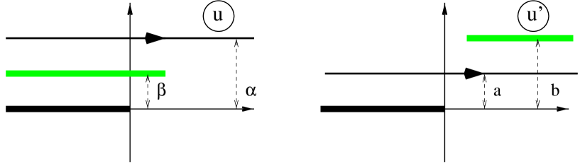
Figure 2: Integration contours in (B9) if $t_{23}>0$, indicated as oriented full lines. The thick black lines indicate the fixed cuts on the negative real axis and the grey lines indicate the moving cuts which occur for $u-u^{\prime}+{\rm i}v$ real negative. On the left the contour is shown when one first integrates over $u$, with $\alpha=\frac{r_{13}^{2}}{2t_{13}}$ and $\beta=\frac{r_{23}^{2}}{2t_{23}}-v$. On the right one integrates first over $u^{\prime}$, with $a=\frac{r_{23}^{2}}{2t_{23}}$ and $b=\frac{r_{13}^{2}}{2t_{13}}+v$.

First, we consider the case $t_{23}>0$. Then $t_{13}>0$ as well and from (B7) one also has $v\geq 0$. In figure 2, we show the integration contours in the complex plane, when the integral over $u$ or $u^{\prime}$, respectively, is performed first. Because of the inequality (B10), the contours never cross the moving cuts. Therefore, if one integrates first over $u$, the contour can be moved freely in the upper half plane above the movable cut and consequently, $I$ must be independent of $\frac{r_{13}^{2}}{2t_{13}}$. On the other hand, if one integrates first over $u^{\prime}$, the contour can be moved freely between the singularities and $I$ is independent of $\frac{r_{23}^{2}}{2t_{23}}$. Therefore $I=I(v;{\cal M}_{1},{\cal M}_{2},x_{1},x_{2},x_{3})$ and we have the integral representation

$$I=\int_{\mathbb{R}+{\rm i}\varepsilon}\!{\rm d}u\,\int_{\mathbb{R}+{\rm i}\varepsilon^{\prime}}\!{\rm d}u^{\prime}\;e^{-{\rm i}{\cal M}_{1}u-{\rm i}{\cal M}_{2}u^{\prime}}\,\left(u-u^{\prime}+{\rm i}v\right)^{-x_{12,3}/2}\,{u^{\prime}}^{-x_{23,1}/2}\,u^{-x_{13,2}/2}$$ (B11)

with $\varepsilon,\varepsilon^{\prime}\gtrsim 0$, at least if $v>0$.

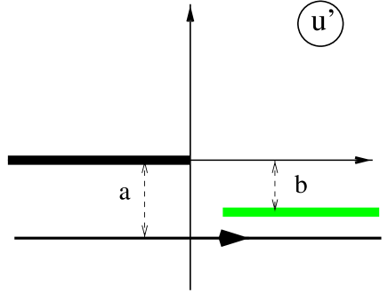
Figure 3: Integration contour in (B9) if $t_{23}<0$. The notation is the same as in figure 2.

Second, we consider the case $t_{23}<0$. We shall show that $I=0$ provided $x_{2}>0$. It is convenient to carry out first the integration over $u^{\prime}$. The contour together with the cuts is shown in figure 3. The position of the contour relative to the cuts follows from (B10) and allows one to close the contour in the lower half plane (the relative position of the cuts depends on the values of the coordinates but does not matter). We now show that the integral

$$J=\int_{\mathbb{R}+{\rm i}\gamma}\!{\rm d}u^{\prime}\,(\alpha+{\rm i}\beta-u^{\prime})^{-x}{u^{\prime}}^{-y}e^{-{\rm i}u^{\prime}}$$ (B12)

vanishes for all real values of $\alpha,\beta$ and $\gamma$ such that $\gamma>\beta$ and if $x+y>0$. That will imply $I=0$ under the stated conditions. In order to see this, consider the contour integral $\oint_{\mathfrak{C}}\!{\rm d}u^{\prime}\>\left(\alpha+{\rm i}\beta-u^{\prime}\right)^{-x}{u^{\prime}}^{-y}e^{-{\rm i}u^{\prime}}$ The contour $\mathfrak{C}$ runs along $\mathbb{R}+{\rm i}\gamma$ and is closed by a semi-circle of radius $R$ in the lower half-plane. The condition $\gamma>\beta$ ensures that the cuts lie on the outside of $\mathfrak{C}$ and therefore, the contour integral vanishes. We introduce polar coordinates $u^{\prime}=Re^{-{\rm i}\theta}$ and estimate the contribution $J_{\rm inf}$ of the lower arc

$$\left|J_{\rm inf}\right|\leq R^{1-x-y}\int_{0}^{\pi}\!{\rm d}\theta\,e^{-R\sin\theta}B^{-x/2}$$ (B13)

where $B$ is defined below. Because of the estimate

$$B:=\left(1-\frac{\alpha+{\rm i}\beta}{R}e^{{\rm i}\theta}\right)\left(1-\frac{\alpha-{\rm i}\beta}{R}e^{-{\rm i}\theta}\right)\leq\left(1+\frac{|\alpha|}{R}\right)^{2}+\left(1+\frac{|\beta|}{R}\right)^{2}\leq 3$$ (B14)

which holds for $R$ sufficiently large, we have

$$\left|J_{\rm inf}\right|\leq 3^{-x/2}R^{1-x-y}\int_{0}^{\pi}\!{\rm d}\theta\,e^{-R\sin\theta}\leq 3^{-x/2}\pi R^{-x-y}$$ (B15)

which tends to zero as $R\to\infty$ provided $x+y>0$, hence $J=0$. Finally, the exponents $x,y$ in $J$ are related to the scaling dimensions $x+y=(x_{12,3}+x_{23,1})/2=x_{2}>0$.

In conclusion, the integral $I$ vanishes if $t_{12}>0$ and $t_{23}<0$ and will therefore contain a factor $\Theta(t_{23})$. By symmetry between $t_{1}$ and $t_{2}$, the case $t_{12}<0$ will produce a factor $\Theta(t_{13})$ provided $x_{1}>0$. The scaling function $\Phi_{12,3}(v)$ in eq. (5) can be identified with the integral $I$ in (B11) and the assertion is proven.

Appendix C. On parabolic subalgebras

We recall here the definition of parabolic subalgebras of a complex simple Lie algebra ${\mathfrak{g}}$, see [40]. The presentation is somewhat simpler than in the general case since for complex ${\mathfrak{g}}$, the compact part and the non-compact part of the Cartan decomposition may be chosen to be the same up to multiplication by ${\rm i}$.

Let ${\mathfrak{g}}$ be a complex simple Lie algebra of rank $r$, ${\mathfrak{h}}$ a complex Cartan subalgebra of ${\mathfrak{g}}$ and $\Delta$ the associated root system. One chooses a basis of simple roots $\Pi=\{\alpha_{1},\ldots,\alpha_{r}\}$ and denotes by $\Delta_{+}\supset\Pi$ the associated set of positive roots. If $\alpha\in\Delta$ is a root, then ${\mathfrak{g}}_{\alpha}\subset{\mathfrak{g}}$ will be the corresponding root space. We shall also use the notation ${\mathfrak{n}}=\sum_{\alpha\in\Delta_{+}}{\mathfrak{g}}_{\alpha}$ for the subalgebra of ${\mathfrak{g}}$ made up of all positive root spaces.

The minimal standard parabolic subalgebra ${\mathfrak{s}}_{0}$ of ${\mathfrak{g}}$ (associated with the given choice of ${\mathfrak{h}}$ and $\Delta_{+}$) is defined as

$${\mathfrak{s}}_{0}={\mathfrak{h}}\oplus{\mathfrak{n}}={\mathfrak{h}}\oplus\sum_{\alpha\in\Delta_{+}}{\mathfrak{g}}_{\alpha}.$$ (C1)

A standard parabolic subalgebra of ${\mathfrak{g}}$ is a subalgebra ${\mathfrak{s}}\subset{\mathfrak{g}}$ containing ${\mathfrak{s}}_{0}$. More generally, a parabolic subalgebra is defined to be a subalgebra of ${\mathfrak{g}}$ containing a conjugate of ${\mathfrak{s}}_{0}$.

The standard parabolic subalgebras ${\mathfrak{s}}$ of ${\mathfrak{g}}$ can be classified by means of a powerful result: they are in one-to-one correspondence with the subsets $\Pi_{{\mathfrak{s}}}$ of $\Pi$. Given $\Pi_{{\mathfrak{s}}}\subset\Pi$, here is how one constructs the associated parabolic subalgebra ${\mathfrak{s}}$. Let ${\mathfrak{h}}_{{\mathfrak{s}}}$ be the set of $H\in{\mathfrak{h}}$ such that $\alpha(H)=0$ for all $\alpha\in\Pi_{{\mathfrak{s}}}$, or in other words the orthogonal in ${\mathfrak{h}}$ of $\Pi_{{\mathfrak{s}}}$; ${\mathfrak{m}}_{{\mathfrak{s}}}$ the centralizer of ${\mathfrak{h}}_{{\mathfrak{s}}}$ in ${\mathfrak{g}}$, that is, the set of elements in ${\mathfrak{g}}$ that commute with all elements in ${\mathfrak{h}}_{{\mathfrak{s}}}$; finally ${\mathfrak{n}}_{{\mathfrak{s}}}\subset{\mathfrak{n}}$ the sum of all root spaces associated with positive roots $\alpha\in\Delta_{+}$ that are not identically zero on ${\mathfrak{h}}_{{\mathfrak{s}}}$. Then ${\mathfrak{h}}_{{\mathfrak{s}}}$, ${\mathfrak{m}}_{{\mathfrak{s}}}$ and ${\mathfrak{n}}_{{\mathfrak{s}}}$ are subalgebras of ${\mathfrak{g}}$, with ${\mathfrak{h}}_{{\mathfrak{s}}}\subset{\mathfrak{h}}\subset{\mathfrak{m}}_{{\mathfrak{s}}}$, and ${\mathfrak{s}}$ is the direct sum

$${\mathfrak{s}}={\mathfrak{m}}_{{\mathfrak{s}}}\oplus{\mathfrak{n}}_{{\mathfrak{s}}}.$$ (C2)

It is easily checked from the above definitions that eq. (C2) yields a Lie subalgebra of ${\mathfrak{g}}$, and that $\alpha\in\Pi$ is in $\Pi_{{\mathfrak{s}}}$ if and only if ${\mathfrak{g}}_{-\alpha}\subset{\mathfrak{m}}_{{\mathfrak{s}}}$ – in which case ${\mathfrak{g}}_{\alpha}$ is also included in ${\mathfrak{m}}_{{\mathfrak{s}}}$. So, in particular, one also sees quite easily that ${\mathfrak{s}}$ is indeed a standard parabolic subalgebra. Since the standard parabolic subalgebras are non-conjugate, it is straightforward to see how this classification extends to a classification of all parabolic subalgebras.

The main motivation for the definition of parabolic subalgebras is that, if $G$ is a simple group with Lie algebra ${\mathfrak{g}}$, the pieces that appear in the Plancherel formula for $G$ all come from representations induced from certain standard parabolic subgroups of $G$ (integrating standard parabolic subalgebras).

The case ${\mathfrak{g}}={\mathfrak{sl}}(r+1,\mathbb{C})$ is particularly illuminating. Take ${\mathfrak{h}}$ to be the space of diagonal matrices with vanishing trace. Let $\alpha_{1}=$diag $(1,-1,0,\ldots,0),\ldots,\alpha_{r}=$diag$(0,\ldots,0,1,-1)$ form a basis $\Pi$ of the set of roots, with the usual identification of ${\mathfrak{h}}$ with its dual. We choose a subset $\alpha_{i_{1}},\ldots,\alpha_{i_{s}}$ $(s\leq r)$ of $\Pi$. One says that $i$ connects with $j$ $(1\leq i<j\leq r+1)$ if $\alpha_{i},\alpha_{i+1},\ldots,\alpha_{j-1}\in\Pi_{{\mathfrak{s}}}$. This defines the connected components of the set $\{1,\ldots,r+1\}$. Then diag$(x_{1},\ldots,x_{r+1})\in{\mathfrak{h}}_{{\mathfrak{s}}}$ if and only if $x_{1}+\ldots+x_{r+1}=0$ and $x_{i}=x_{j}$ whenever $i$ and $j$ are connected. Therefore, a diagonal matrix $H$ with vanishing trace is in ${\mathfrak{h}}_{{\mathfrak{s}}}$ if and only if its entries situated in a single connected component of $\{1,\ldots,r+1\}$ are all equal. So, ${\mathfrak{m}}_{{\mathfrak{s}}}$ is the set of block-diagonal matrices with vanishing trace that do not mix the different components.

For illustration, take the example $r=4$ and $\Pi_{{\mathfrak{s}}}=\{\alpha_{1},\alpha_{3},\alpha_{4}\}$. An element $H\in{\mathfrak{h}}_{{\mathfrak{s}}}$ can be written as a diagonal matrix

$$H=\left(\begin{array}[]{ccccc}x_{1}\\ &x_{1}\\ &&x_{2}\\ &&&x_{2}\\ &&&&x_{2}\end{array}\right)\;\;,\;\;\mbox{\rm with $2x_{1}+3x_{2}=0$}$$ (C3)

In turn, elements $M\in{\mathfrak{m}}_{{\mathfrak{s}}}$ and $N\in{\mathfrak{n}}_{{\mathfrak{s}}}$ can be written as

$$M=\left(\begin{array}[]{cc}M_{1}&0\\ 0&M_{2}\end{array}\right)\;\;,\;\;N=\left(\begin{array}[]{cc}0&N_{1}\\ 0&0\end{array}\right)$$ (C4)

where $M_{1},M_{2}$ and $N_{1}$ are, respectively, $2\times 2$, $3\times 3$ and $2\times 3$ matrices and ${\rm tr\ }M_{1}+{\rm tr\ }M_{2}=0$.

It is fairly easy to find the standard parabolic subalgebras in the case studied in section 3, namely ${\mathfrak{g}}={\mathfrak{so}}(5,\mathbb{C})$. Referring to the notations of that section, the chosen basis of simple roots is

$$\alpha_{1}=-e_{2},\ \alpha_{2}=e_{1}+e_{2}.$$ (C5)

In table 1 we list all possible $\Pi_{{\mathfrak{s}}},{\mathfrak{h}}_{{\mathfrak{s}}},{\mathfrak{m}}_{{\mathfrak{s}}},{\mathfrak{n}}_{{\mathfrak{s}}}$ and ${\mathfrak{s}}$.

Table 1: Construction of the standard parabolic subalgebras $\mathfrak{s}$ of the complex Lie algebra $\mathfrak{g}=(\mathfrak{conf}_{3})_{\mathbb{C}}$.

$\Pi_{{\mathfrak{s}}}$	${\mathfrak{h}}_{{\mathfrak{s}}}$	${\mathfrak{m}}_{{\mathfrak{s}}}$	${\mathfrak{n}}_{{\mathfrak{s}}}$	${\mathfrak{s}}$
$\emptyset$	${\mathfrak{h}}$	${\mathfrak{h}}$	${\mathfrak{n}}$	$\widetilde{\mathfrak{age}}_{1}$
$\{\alpha_{1}\}$	$\mathbb{C}N$	${\mathfrak{h}}\oplus\mathbb{C}Y_{-{1\over 2}}\oplus\mathbb{C}V_{+}$	$\mathbb{C}X_{1}\oplus\mathbb{C}M_{0}\oplus\mathbb{C}Y_{{1\over 2}}$	$\widetilde{\mathfrak{alt}}_{1}$
$\{\alpha_{2}\}$	$\mathbb{C}(N-D)$	${\mathfrak{h}}\oplus\mathbb{C}X_{-1}\oplus\mathbb{C}X_{1}$	$\mathbb{C}Y_{-{1\over 2}}\oplus\mathbb{C}Y_{{1\over 2}}\oplus\mathbb{C}M_{0}$	$\widetilde{\mathfrak{sch}}_{1}$
$\{\alpha_{1},\alpha_{2}\}$	$\{0\}$	${\mathfrak{g}}$	$\{0\}$	$(\mathfrak{conf}_{3})_{\mathbb{C}}$

Let us explain how to find the entries in table 1 in the case where $\Pi_{{\mathfrak{s}}}=\{\alpha_{1}\}=\{-e_{2}\}$. Then

$${\mathfrak{h}}_{{\mathfrak{s}}}=\{\lambda N+\mu D\ |\ \alpha_{1}(\lambda N+\mu D)=0\}=\{\lambda N\}=\mathbb{C}N$$ (C6)

where we recall from section 3 that $e_{i}(N)=\delta_{i,1}$ and $e_{i}(D)=\delta_{i,2}$. So

$${\mathfrak{m}}_{{\mathfrak{s}}} = \{X\in{\mathfrak{g}}\ |\ [X,{\mathfrak{h}}_{{\mathfrak{s}}}]=0\}={\mathfrak{h}}\oplus{\mathfrak{g}}_{-e_{2}}\oplus{\mathfrak{g}}_{e_{2}}$$ (C7)

$$= {\mathfrak{h}}\oplus\mathbb{C}Y_{-{1\over 2}}\oplus\mathbb{C}V_{+}.$$

To find ${\mathfrak{n}}_{{\mathfrak{s}}}$, we must determine all positive roots which vanish on ${\mathfrak{h}}_{{\mathfrak{s}}}$. In this case, the only such positive root is $-e_{2}$. Consequently, with the set $\Delta_{+}$ of positive roots given by (3.8)

$${\mathfrak{n}}_{{\mathfrak{s}}}={\mathfrak{g}}_{e_{1}+e_{2}}\oplus{\mathfrak{g}}_{e_{1}}\oplus{\mathfrak{g}}_{e_{1}-e_{2}}=\mathbb{C}X_{1}\oplus\mathbb{C}Y_{{1\over 2}}\oplus\mathbb{C}M_{0}.$$ (C8)