CERN-TH/2003-022

TPI-MINN-03/04, UMN-TH-2129/03

Exact Results in Non-Supersymmetric

Large N Orientifold Field Theories

A. Armoni ^a, M. Shifman ^a,b, G. Veneziano ^a

adi.armoni, michael.shifman, gabriele.veneziano@cern.ch

^a Theory Division, CERN

CH-1211 Geneva 23, Switzerland

^b William I. Fine Theoretical Physics Institute, University of Minnesota,

Minneapolis, MN 55455, USA^⋆

We consider non-supersymmetric large $N$ orientifold field theories. Specifically, we discuss a gauge theory with a Dirac fermion in the anti-symmetric tensor representation. We argue that, at large $N$ and in a large part of its bosonic sector, this theory is non-perturbatively equivalent to ${\cal N}=1\$SYM, so that exact results established in the latter (parent) theory also hold in the daughter orientifold theory. In particular, the non-supersymmetric theory has an exactly calculable bifermion condensate, exactly degenerate parity doublets, and a vanishing cosmological constant (all this to leading order in $1/N$).

 
^⋆ Permanent address.

1 Introduction

Gauge field theories at strong coupling are of great importance in particle physics. Exact results in gauge theories at strong coupling have a special weight. In the last few years supersymmetry (SUSY) proved to be a guiding principle (see e.g. [1]) providing deep insights in gauge dynamics. Recently it was suggested that a large number of symmetry relations valid in supersymmetric theories remain valid in the large $N$ limit in non-supersymmetric daughter theories obtained from the parent one through orbifoldization [2]. The most popular (non-SUSY) orbifolds are ${\bf Z}_{2}\$, or ${\bf Z}_{k}\$in general [3, 4, 5]. In particular, in the last paper it was argued that the superpotential of SUSY gluodynamics [6],

$$W(S)=N(S\log S/\Lambda^{3}-S)\,,\qquad S=\lambda\lambda+...\,,$$ (1)

can be in a sense extended to its ${\bf Z}_{2}\$orbifold. This is equivalent to the statement that the daughter theory has $N$ vacua labeled by a bifermion condensate

$$\langle\lambda\lambda\rangle_{k}=N\Lambda^{3}\exp\left(i{2\pi k\over N}\right).$$ (2)

While the planar equivalence is certainly true in perturbation theory [7, 8] its nonperturbative status is being debated; a number of arguments pro and con can be found in the literature [3, 4, 5].

The purpose of this work is to present a non-supersymmetric daughter (different from the ${\bf Z}_{k}\$orbifolds) for which the large $N$ equivalence between the parent SUSY theory and the daughter non-supersymmetric one at nonperturbative level rests on a more solid ground than in the case of the ${\bf Z}_{k}\$orbifolds. This “orientifold field theory” was suggested in Refs. [9, 10] in a somewhat different context. One of its advantages over more popular ${\bf Z}_{k}\$orbifolds is the absence in it of the twisted sector.

The field content of the orientifold gauge field theory differs from the one of its parent theory, U($N$) SUSY gluodynamics, in that the gluinos are replaced by massless Dirac fermions in the rank-two antisymmetric tensor representation of U($N$) (denoted by $\vbox{\vbox{\hrule height=0.3pt\hbox{\vrule width=0.3pt,height=6.4pt\kern 6.4pt\vrule width=0.3pt} \hrule height=0.3pt\kern-0.3pt\hrule height=0.3pt\hbox{\vrule width=0.3pt,height=6.4pt\kern 6.4pt\vrule width=0.3pt} \hrule height=0.3pt}}+\overline{\vbox{\vbox{\hrule height=0.3pt\hbox{\vrule width=0.3pt,height=6.4pt\kern 6.4pt\vrule width=0.3pt} \hrule height=0.3pt\kern-0.3pt\hrule height=0.3pt\hbox{\vrule width=0.3pt,height=6.4pt\kern 6.4pt\vrule width=0.3pt} \hrule height=0.3pt}}}$). The total number of (say) left handed fermions is thus $N(N-1)$ in the daughter theory and $N^{2}$ in the parent theory and agrees to leading order in $1/N$. Similarly, one can discuss a theory with a Dirac fermion in the symmetric representation ($\raisebox{-0.5pt}{\hbox{\rule{0.4pt}{6.5pt}\hskip-0.4pt\rule{6.5pt}{0.4pt}\hskip-6.5pt\rule[6.5pt]{6.5pt}{0.4pt}}\rule[6.5pt]{0.4pt}{0.4pt}\hskip-0.4pt\rule{0.4pt}{6.5pt}}\hskip-0.4pt\raisebox{-0.5pt}{\hbox{\rule{0.4pt}{6.5pt}\hskip-0.4pt\rule{6.5pt}{0.4pt}\hskip-6.5pt\rule[6.5pt]{6.5pt}{0.4pt}}\rule[6.5pt]{0.4pt}{0.4pt}\hskip-0.4pt\rule{0.4pt}{6.5pt}}+\overline{\raisebox{-0.5pt}{\hbox{\rule{0.4pt}{6.5pt}\hskip-0.4pt\rule{6.5pt}{0.4pt}\hskip-6.5pt\rule[6.5pt]{6.5pt}{0.4pt}}\rule[6.5pt]{0.4pt}{0.4pt}\hskip-0.4pt\rule{0.4pt}{6.5pt}}\hskip-0.4pt\raisebox{-0.5pt}{\hbox{\rule{0.4pt}{6.5pt}\hskip-0.4pt\rule{6.5pt}{0.4pt}\hskip-6.5pt\rule[6.5pt]{6.5pt}{0.4pt}}\rule[6.5pt]{0.4pt}{0.4pt}\hskip-0.4pt\rule{0.4pt}{6.5pt}}}$). As we will see, this theory lives on a brane configuration of type 0A string theory [9] which consists of NS5 branes, D4 branes and an orientifold plane — hence the name “orientifold field theory.” The daughter theory in our case is a much closer cousin of ${\cal N}=1\$SYM than the ${\bf Z}_{2}\$orbifold. Indeed, the gauge groups in the parent and daughter theories are the same, and no rescaling of the gauge couplings is needed.

Assuming that both theories are in the confining regime , we will show that in the large $N$ limit many results and symmetry relations that were obtained for ${\cal N}=1\$SYM hold also for the above orientifold field theory. One specific quantity is the bifermion condensate (2). It labels distinct vacua. The number of vacua turns out to be the same in the parent and daughter theories, $N$. Another result is the vanishing of the vacuum energy density in the daughter theory.

We would like to emphasize that the spectrum of the orientifold field theory does not coincide with that of ${\cal N}=1\$SYM in the large $N$ limit. In particular, there is no SUSY. While the composite color-singlet hadrons of ${\cal N}=1\$are fermi-bose degenerate, the composite color-singlet hadrons of the orientifold field theory are purely bosonic.

The organization of this paper is as follows: in Sect. 2 we present our main result — the perturbative and nonperturbative equivalence. In Sect. 3 we briefly present the string theory realization of the theory in its conjectured relation to M-theory. In Sect. 4 we compare our analysis and results with those referring to ${\bf Z}_{k}\$orbifold field theories and summarize conclusions.

2 Orientifold field theory and ${\cal N}=1\$SYM

In this section we will argue that in the $N\to\infty$ limit there is a sector in the orientifold theory exactly identical to ${\cal N}=1\$SYM and, therefore, exact results on the IR behavior of this theory can be obtained.

The parent theory is ${\cal N}=1\$SUSY gluodynamics with the gauge group U($N$). In the large $N$ limit the U(1) factor is irrelevant. The daughter theory has the same gauge group, and the same gauge coupling . The gluino field $\lambda^{i}_{j}$ is replaced by two Weyl spinors $\lambda_{[ij]}$ and $\xi^{[ij]}$. We can combine the Weyl spinors into one Dirac spinor, either $\Psi_{[ij]}$ or $\Psi^{[ij]}$. Note that the number of fermionic degrees of freedom is $N^{2}-N$, as in the parent theory in the large $N$ limit.

The hadronic (color-singlet) sectors of the theories are different. In the parent theory composite fermions with mass scaling as $N^{0}$ exist, and moreover, they are degenerate with their bosonic SUSY counterparts. In the daughter theory any interpolating color-singlet current with the fermion quantum numbers contains a number of constituents growing with $N$. Hence at $N=\infty$ the spectrum contains only bosons.

Classically the parent theory has just an $R$ symmetry corresponding to chiral rotations of the gluino field. Instantons break this symmetry down to ${\bf Z}_{2N}\$. The daughter theory has, on top, a conserved anomaly free current

$$\bar{\lambda}_{\dot{\alpha}}\lambda_{\alpha}-\bar{\xi}_{\dot{\alpha}}\xi_{\alpha}\,.$$ (3)

In terms of the Dirac spinor this is the vector current $\bar{\Psi}\gamma_{\mu}\Psi$. If the corresponding charge is denoted by $Q$, in the color-singlet bosonic sector $Q=0$, with necessity. Then the only global symmetry which remains in both theories is ${\bf Z}_{2N}\$ spontaneously broken down to ${\bf Z}_{2}\$by the respective bifermion condensates. This explains the existence of $N$ vacua in both cases. We will compare the bosonic sectors of the parent and daughter theories. Note that in the daughter theory the part of the bosonic sector probed by the operators of the type (3), which have no analogs in the parent theory, is inaccessible.

Let us start from perturbative consideration. The general argument for any orbifold/orientifold field theory is given in [7, 8]. Let us see how it works in our orientifold field theory. The Feynman rules of the planar theory are shown in Fig.1. The difference between the orientifold theory and ${\cal N}=1\$is that the arrows on the fermionic lines point in the same direction, since the fermion is in the antisymmetric representation, in contrast to the supersymmetric theory where the gaugino is in the adjoint representation and the arrows point in the opposite directions. This difference between the two theories does not affect planar graphs provided each gaugino line is replaced by the sum of $\lambda_{[..]}$ and $\lambda^{[..]}$.

Figure 1: (a) The fermionic propagator and the vertex. (b) ${\cal N}=1\$SYM. (c) The non-SUSY theory.

There is a one-to-one correspondence between the planar graphs of the two theories. Diagrammatically this works as follows (see, for example, Fig. 2). Consider any planar diagram of the daughter theory: by definition of planarity it can be drawn on a sphere. The fermionic propagators form closed, non-intersecting loops that divide the sphere into regions. Each time we cross a fermionic line the orientation of color-indices loops (each one producing a factor $N$) changes from clock to anti-clock wise, and vice-versa, as easily seen in Fig. 2c. Thus, the fermionic loops allow to attribute to each one of the above regions a binary label (say $\pm 1$) according to whether the color loops go clock- or anti-clock-wise in that region. Now imagine that the orientation of color loops in all regions with the $-1$ label is reversed. We will get a planar diagram of the SYM theory in which all color loops go, by convention, clock-wise. The number associated with both diagrams will be the same since the diagrams inside each region always contain an even number of powers of $g$ so that the relative minus signs of Fig. 1 do not matter.

Let us illustrate how this works, say, for the inside part of the graph in Fig. 2b. In the parent theory we have the color factor Tr $(T^{a}T^{b}T^{c})\,f^{abc}$ while in the daughter one Tr $(\bar{T}^{a}\bar{T}^{b}\bar{T}^{c})\,f^{abc}$ where $\bar{T}=-\tilde{T}$ and the tilde marks the transposed matrix . Using the fact that

$$[T^{a}T^{b}]=if^{abc}T^{c}\quad\mbox{and}\quad[\bar{T}^{a}\bar{T}^{b}]=if^{abc}\bar{T}^{c}$$

we immediately come to the conclusion that the above two expressions coincide.

Figure 2: (a) A typical planar contribution to the vacuum polarization. (b) For ${\cal N}=1\$SYM. (c) For the non-SUSY theory.

Thus, all perturbative results that we know of in ${\cal N}=1\$SYM apply for the orientifold model as well. For example, the $\beta$ function of the orientifold field theory is

$$\beta=-\frac{1}{2\pi}\,\frac{3N\alpha^{2}}{1-(N\alpha)/(2\pi)}\left\{1+O\left(\frac{1}{N}\right)\right\},$$ (4)

where $\alpha={g^{2}\over 4\pi}$. In the large $N$ limit it coincides with the ${\cal N}=1\$SYM result [11]. Note that the corrections are $1/N$ rather than $1/N^{2}$. For instance, the exact first coefficient of the $\beta$ function is $-3N-4/3$ versus $-3N$ in the parent theory.

Now let us argue that the perturbative argument can be elevated to nonperturbative level in the case at hand. A heuristic argument in favor of the nonperturbative equivalence is that the coincidence of all planar graphs of the two theories implies that the relevant Casimir operators of the two representations are equivalent in the large $N$ limit. The partition functions of the two theories depend on the Casimir operators and therefore must coincide as well.

A more formal line of reasoning is as follows. It is essential that the fermion fields enter bilinearly in the action, and that for any given gauge field configuration in the parent theory there is exactly the same configuration in the daughter one. (The latter feature is absent in the ${\bf Z}_{k}\$orbifolds.) Our idea is to integrate out fermion fields for any fixed gluon field configuration, which yields respective determinants, and then compare them.

Consider the partition function of ${\cal N}=1\$SYM,

$${\cal Z}_{0}=\int{\cal D}A\,{\cal D}\lambda\,\exp\left(iS[A,\lambda,J]\right)\,,$$ (5)

where $J$ is any source coupled to color-singlet gluon operators (we will discuss color-singlet fermion bilinears later).

For any given gluon field, upon integrating out the gaugino field, we obtain

$${\cal Z}_{0}=\int{\cal D}A\,\exp\left(iS[A,J]\right)\det\left(\not{\hbox{\kern-2.0pt${\partial}$}}+\not{\hbox{\kern-2.0pt${A}$}}^{a}T^{a}_{\rm adj}\right),$$ (6)

where $T^{a}_{\rm adj}$ is a generator of the adjoint representation.

If one integrates out the fermion fields of the non-supersymmetric orientifold theory, at fixed $A$, one arrives at a similar expression, but with the generators of the anti-symmetric representation instead of the adjoint, $T^{a}_{\rm adj}\rightarrow T^{a}_{\rm as}$.

To compare the fermion determinants in the parent and daughter theories (assuming that the gauge field configuration $A_{\mu}^{a}(x),\,\,\,a=1,...,N^{2},$ is the same and fixed) we must cast both fermion operators in similar forms. To this end we will extend both theories. In the parent one we introduce the second adjoint Weyl fermion $\xi^{i}_{j}$ and combine two Weyl fermions into one Dirac adjoint fermion $\Psi^{i}_{j}$. The determinant in this extended theory is the square of the original one; we assume that taking the square root at the end is harmless.

In the daughter theory instead of $\Psi^{[ij]}$, we will work with the reducible representation, combining both symmetric and antisymmetric, $\Psi^{ij}$ (no (anti)symmetrization over the color indices). Then the number of the fermion Dirac fields is the same as in the extended parent. Again, as in the previous case, the determinant in the extended daughter theory is the square of the original one. For infrared regularization we will introduce small mass terms, assuming that the vanishing mass limit is smooth.

Next, we will make use of the fact that

$$T^{a}_{adj}\sim T^{a}_{\raisebox{-0.5pt}{\hbox{\rule{0.4pt}{6.5pt}\hskip-0.4pt\rule{6.5pt}{0.4pt}\hskip-6.5pt\rule[6.5pt]{6.5pt}{0.4pt}}\rule[6.5pt]{0.4pt}{0.4pt}\hskip-0.4pt\rule{0.4pt}{6.5pt}}\,\times\,\overline{\raisebox{-0.5pt}{\hbox{\rule{0.4pt}{6.5pt}\hskip-0.4pt\rule{6.5pt}{0.4pt}\hskip-6.5pt\rule[6.5pt]{6.5pt}{0.4pt}}\rule[6.5pt]{0.4pt}{0.4pt}\hskip-0.4pt\rule{0.4pt}{6.5pt}}}}=T^{a}_{\raisebox{-0.5pt}{\hbox{\rule{0.4pt}{6.5pt}\hskip-0.4pt\rule{6.5pt}{0.4pt}\hskip-6.5pt\rule[6.5pt]{6.5pt}{0.4pt}}\rule[6.5pt]{0.4pt}{0.4pt}\hskip-0.4pt\rule{0.4pt}{6.5pt}}}\otimes 1+1\otimes T^{a}_{\overline{\raisebox{-0.5pt}{\hbox{\rule{0.4pt}{6.5pt}\hskip-0.4pt\rule{6.5pt}{0.4pt}\hskip-6.5pt\rule[6.5pt]{6.5pt}{0.4pt}}\rule[6.5pt]{0.4pt}{0.4pt}\hskip-0.4pt\rule{0.4pt}{6.5pt}}}}\,,$$ (7)

and

$$T^{a}_{d}=T^{a}_{\raisebox{-0.5pt}{\hbox{\rule{0.4pt}{6.5pt}\hskip-0.4pt\rule{6.5pt}{0.4pt}\hskip-6.5pt\rule[6.5pt]{6.5pt}{0.4pt}}\rule[6.5pt]{0.4pt}{0.4pt}\hskip-0.4pt\rule{0.4pt}{6.5pt}}}\otimes 1+1\otimes T^{a}_{\raisebox{-0.5pt}{\hbox{\rule{0.4pt}{6.5pt}\hskip-0.4pt\rule{6.5pt}{0.4pt}\hskip-6.5pt\rule[6.5pt]{6.5pt}{0.4pt}}\rule[6.5pt]{0.4pt}{0.4pt}\hskip-0.4pt\rule{0.4pt}{6.5pt}}}\,,$$ (8)

or

$$T^{a}_{d}=T^{a}_{\overline{\raisebox{-0.5pt}{\hbox{\rule{0.4pt}{6.5pt}\hskip-0.4pt\rule{6.5pt}{0.4pt}\hskip-6.5pt\rule[6.5pt]{6.5pt}{0.4pt}}\rule[6.5pt]{0.4pt}{0.4pt}\hskip-0.4pt\rule{0.4pt}{6.5pt}}}}\otimes 1+1\otimes T^{a}_{\overline{\raisebox{-0.5pt}{\hbox{\rule{0.4pt}{6.5pt}\hskip-0.4pt\rule{6.5pt}{0.4pt}\hskip-6.5pt\rule[6.5pt]{6.5pt}{0.4pt}}\rule[6.5pt]{0.4pt}{0.4pt}\hskip-0.4pt\rule{0.4pt}{6.5pt}}}}\,.$$ (9)

The subscript d stands for “daughter.” Let us now introduce, as an auxiliary object,

$$F(A,B)={\rm tr}\,\ln\left(\not{\hbox{\kern-2.0pt${\partial}$}}+\not{\hbox{\kern-2.0pt${A}$}}^{a}(T^{a}_{\raisebox{-0.5pt}{\hbox{\rule{0.4pt}{6.5pt}\hskip-0.4pt\rule{6.5pt}{0.4pt}\hskip-6.5pt\rule[6.5pt]{6.5pt}{0.4pt}}\rule[6.5pt]{0.4pt}{0.4pt}\hskip-0.4pt\rule{0.4pt}{6.5pt}}}\otimes 1)+\not{\hbox{\kern-2.0pt${B}$}}^{a}(1\otimes T^{a}_{\overline{\raisebox{-0.5pt}{\hbox{\rule{0.4pt}{6.5pt}\hskip-0.4pt\rule{6.5pt}{0.4pt}\hskip-6.5pt\rule[6.5pt]{6.5pt}{0.4pt}}\rule[6.5pt]{0.4pt}{0.4pt}\hskip-0.4pt\rule{0.4pt}{6.5pt}}}})\right)\,,$$ (10)

and notice that (at large$N$) $F$ is invariant under separate gauge transformations acting on $A^{a}$ and $B^{a}$. Using the fact that the Wilson loop operators ${\cal W}_{\cal C}(A)={\rm tr}\,P\,\exp\left(i\int_{\cal C}A\right)$ form a complete set of gauge invariant operators, we can write

$$\exp\left\{F(A,B)\right\}=\sum_{\cal C,C^{\prime}}\alpha_{\cal C,C^{\prime}}{\cal W}_{\cal C}(A){\cal W}_{\cal C^{\prime}}(B).$$ (11)

The partition function of ${\cal N}=1\$SYM can be written, at large $N$, as

$${\cal Z}_{0}=\int{\cal D}A\,{\cal D}B\,\delta(A-B)\,\exp\left\{-\mbox{$\frac{1}{2}$}(S[A]+S[B])\right\}\sum_{\cal C,C^{\prime}}\alpha_{\cal C,C^{\prime}}{\cal W}_{\cal C}(A){\cal W}_{\cal C^{\prime}}(B).$$ (12)

Now let us turn to the daughter theory. The partition function of the orientifold theory, at large $N$, can be written as (12), but with the orientations of the Wilson loops ${\cal W}(B)$ reversed, since we replace the fundamental fermions by anti-fundamental fermions. This gives

$${\cal W}_{\cal C^{\prime}}\to{\cal W}_{\bar{\cal C^{\prime}}}=\left\{{\cal W}_{\cal C^{\prime}}\right\}^{*}\,.$$

Moreover, ${\cal W}_{\cal C^{\prime}}$ is real, and this is why reversing the orientation should not change the value of the partition function.

Let us present now a more detailed derivation which relies on the fact that at large $N$ the two kinds of gluons do not interact with each other. The partition function (12) can be written as

$${\cal Z}_{0}=\int{\cal D}A\,\exp\left\{-S[A]+F(A,B=A)\right\}.$$ (13)

Let us expand $\exp(-S)$

$$\exp\left\{-S[A]\right\}=\sum_{n}{(-1)^{n}\over n!}\left\{S[A]\right\}^{n}.$$ (14)

At $N\rightarrow\infty$, the vertices or propagators coming from each factor of $S$ cannot connect $A$ with $B$. Thus, we have

$$S^{n}\sim\sum_{k=0}^{n}C_{k}S^{k}[A]S^{n-k}[B],$$ (15)

where the $\sim$ sign means “can be replaced by” and $C_{k}$ is a combinatorial factor corresponding to the various choices of picking $k$ out of $n$,

$$C_{k}={n!\over k!(n-k)!}\,.$$

Then

$$\exp(-S) \sim \sum_{n}{(-1)^{n}\over n!}\sum_{k}{n!\over k!(n-k)!}\left\{S[A]\right\}^{k}\left\{S[B]\right\}^{n-k}$$ (16)

$$= \exp(-S[A]-S[B]).$$

Thus, we conclude that $\exp(-S)$ acts as $\exp(-S[A]-S[B])$ and, at large $N$, we can think of the partition function as if we actually have two gauge fields. Thus, at large $N$, Eq. (12) becomes

$${\cal Z}_{0}=\sum_{\cal C,\cal C^{\prime}}\alpha_{\cal C,\cal C^{\prime}}\left\langle{\cal W}_{\cal C}\right\rangle\left\langle{\cal W}_{\cal C^{\prime}}\right\rangle.$$ (17)

In order to pass to the daughter theory one has to replace $B=B^{a}T^{a}_{\overline{\raisebox{-0.5pt}{\hbox{\rule{0.4pt}{6.5pt}\hskip-0.4pt\rule{6.5pt}{0.4pt}\hskip-6.5pt\rule[6.5pt]{6.5pt}{0.4pt}}\rule[6.5pt]{0.4pt}{0.4pt}\hskip-0.4pt\rule{0.4pt}{6.5pt}}}}$ by $B=B^{a}T^{a}_{\raisebox{-0.5pt}{\hbox{\rule{0.4pt}{6.5pt}\hskip-0.4pt\rule{6.5pt}{0.4pt}\hskip-6.5pt\rule[6.5pt]{6.5pt}{0.4pt}}\rule[6.5pt]{0.4pt}{0.4pt}\hskip-0.4pt\rule{0.4pt}{6.5pt}}}$. But $B$ is a dummy variable and, hence, this substitution will not change the value of the partition function. Though we used a perturbative intuition in order to arrive to the factorization of either the Wilson loops in (12) or the action in Eq. (16) we believe that this is an exact property of the partition function. Note also that the factorization in the partition function follows immediately from the existence of a master field [12]. Thus, given the existence of a large $N$ master field, the equivalence of the parent and daughter theories is proven.

Another line of reasoning supporting non-perturbative planar equivalence of the parent and orientifold theories is based on lattice formulations of both theories. If one examines strong coupling diagrams for, say, a Wilson loop on the lattice, one readily concludes that the large $N$ diagrams of the two theories can be put in a one-to-one correspondence and agree to leading order in $1/N$.

For all these reasons we believe that the full equivalence of these two theories takes place in the large $N$ limit, for quantities which do not involve fermion external legs. The equivalence is nonperturbative. An immediate result is that the vacuum energy of the orientifold theory is zero in the large $N$ limit (or at finite $N$ it is $1/N$ relatively to a natural $N^{2}$ behavior). To be more precise, the expected dependence of the vacuum energy on the UV cut-off and $N$ is generically

$$\rho=\Lambda_{UV}^{4}N^{2}(c_{0}+c_{1}/N+c_{2}/N^{2}+...).$$ (18)

In the present theory $c_{0}=0$ while, generically, $c_{1},c_{2},...$ are non-zero. Namely, the vacuum energy is zero only in the planar theory. If one keeps the combination $\Lambda_{UV}^{4}N^{2}$ fixed then the limiting theory has a zero vacuum energy. While this is an almost trivial statement in the UV, simply because of the equivalence of the planar graphs, it is highly nontrivial from the IR point of view. The daughter theory hadronic spectrum consists of bosons only, since it is impossible to form light color-singlet fermions. Nonetheless one should remark that contributions to the cosmological constant from color-singlet loops only enter at the level of the genus-1 (torus) diagrams. These are already O($1/N^{2}$) down with respect to the leading contribution to the cosmological constant (which vanishes) and O($1/N$) relative to the presumed leading non-vanishing contribution in the daughter theory.

In order to go beyond the equivalence of vacuum diagrams and correlators with external gluonic sources we have to understand how the above argument can be extended if we add fermionic bilinear sources.

It looks quite obvious that sources coupled to $\lambda\lambda\pm\bar{\lambda}\bar{\lambda}$ in the parent theory can be mapped into sources coupled to $\bar{\Psi}(1\pm\gamma_{5})\Psi$ in the daughter theory. This will be enough to prove the equality of condensates in the two theories and the $x$-independence of certain correlators, hence the parity-doublet structure of the spectrum in both theories (see below). In particular, a mass terms can be added to both theories without spoiling their large $N$ equivalence. Although we have not made a systematic study of this problem it looks that many other fermionic bilinears (FB) — involving the gluon field as well — can be mapped in the two theories so that

$$W_{\rm SYM}(J_{\rm glue}^{i},J_{FB}^{j})=W_{\rm ori}(J_{\rm glue}^{i},\tilde{J}_{FB}^{j})(1+O(1/N))$$ (19)

with an explicit dictionary relating $J_{FB}^{j}$ and $\tilde{J}_{FB}^{j}$. An example of such a pair is

$$\left(G_{\alpha\beta}\right)^{i}_{j}\left(\lambda_{\alpha}\right)^{k}_{i}\left(\lambda_{\beta}\right)^{j}_{k}\leftrightarrow\left(G_{\alpha\beta}\right)^{i}_{j}\left(\lambda_{\alpha}\right)_{[ik]}\left(\xi_{\beta}\right)^{[kj]}\,,$$ (20)

where $\left(G_{\alpha\beta}\right)^{i}_{j}$ is the gluon field strength tensor.

As was mentioned, we can derive the bifermion condensate $\langle\lambda\xi\rangle\neq 0$ in the daughter theory starting from $\langle\lambda\lambda\rangle\neq 0$ in the parent one, hence

$$\langle\lambda\xi\rangle_{k}=N\Lambda^{3}\exp\left(i{2\pi k\over N}\right)\,,$$

as in Eq. (2).

Another property which is inherited by the daughter theory is the constancy of the chiral correlator

$$\langle\lambda\xi(x_{1})\,\,\lambda\xi(x_{2})\,\,...\,\,\lambda\xi(x_{n})\rangle={\rm const.}$$ (21)

Physically it is related to the mass degeneracy of scalar and pseudoscalar mesons.

It should be stressed that in ${\bf Z}_{k}\$orbifolds some background gauge field configurations are present in the parent theory and absent in the daughter one, so that comparison of the fermion determinants does not prove nonperturbative equivalence.

To summarize, we can relate many correlators which involve even number of fermions and/or gluon operators (hence, the corresponding hadron spectra). However, the parent and daughter theories differ from each other in the sector of odd number of fermions. For example, there is a gauge invariant three-fermions state in ${\cal N}=1\$SYM. Such a state does not exist in the orientifold theory. Remember also that the sector of the daughter theory probed by the operators of the type (3) is not accessible for predictions.

3 The relation with type 0A string theory and M-theory

In this section we show that our orientifold field theory has a simple realization in type 0A string theory. Type 0A/B are bosonic closed string theories with a low-energy spectrum which consist of the universal NS-NS sector, a tachyon and a doubled set of R-R forms with respect to type IIA/B string theories. Type 0B string theory has three kinds of orientifolds [13, 14]. We will be mostly interested in the nontachyonic one [13, 14]. Consider the action $\Omega(-1)^{f_{R}}$, namely the world-sheet parity combined with the world-sheet fermion number. The NS-NS vacuum is odd with respect to this action and, therefore, it is removed from the spectrum. Thus, the bulk theory is tachyon free. In addition this orientifold removes half of the R-R fields so that the theory now has only one set of R-R fields, as in the type IIB theory. In order to remove R-R tadpoles one has to introduce 32 D9 branes. The field theory on the D9 branes is a 10 dimensional $U(32)$ gauge theory with an antisymmetric fermion.

One can perform a sequence of T dualities to obtain a system of D4 branes and O4 plane. Moreover, a brane configuration which consists of NS5 branes and an O4 plane as in Fig. 3, leads [10] to our “orientifold field theory”.

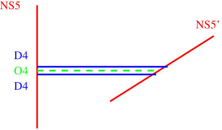
Figure 3: The type 0A brane configuration. The solid lines denote D4 branes. The dashed line denotes the orientifold 4-plane.

We would like to use the relation of type 0A string theory to M-theory to study the strong coupling regime of the orientifold theory at large $N$. This argument is certainly not a proof and we present it just to indicate that our results in Sect. 2 are in agreement with the string theory picture.

Similarly to type IIA string theory, type 0A can be obtained from M-theory by a compactification of the eleventh dimension on a Scherk-Schwarz circle [15]. By using this conjecture we can lift the brane configuration (Fig. 3) to M-theory, similarly to the lift of the analogous type IIA brane configuration [16, 17, 18]. Note that the presence of the orientifold plane can be neglected in the large $N$ limit, since its R-R charge is negligible with respect to the R-R charge of the branes ($N$). Similarly to the type IIA situation we will obtain a smooth M5 brane and the resulting curve (the shape of the M5) will be the same as the curve of ${\cal N}=1\$SYM [18]

$$S^{N}=1.$$ (22)

The meaning of this curve is that there are $N$ vacua with the bifermion condensate (2) as the order parameter, in agreement with our field theory results.

4 Discussion and conclusions

One of the goals of this section is to compare in more detail the results that are obtained in this work for orientifold field theories with the previous results for orbifold field theories.

In order to be concrete let us discuss, as an example, the ${\bf Z}_{2}\$orbifold theory (see Table). This theory as well has a realization in type 0A theory [9]. It lives on a brane configuration of type 0A which consists of ‘electric’ and ‘magnetic’ D-branes, hence the labels ‘e’ and ‘m’ in the Table.

Let us divide the operators in the ${\bf Z}_{2}\$orbifold theory to operators that are invariant (even) under the exchange of the labels ‘e’ and ‘m’ and operators which are odd under this exchange. The first are called “untwisted operators,” the second “twisted operators.” For example, the operator ${\cal O}^{+}={\rm tr}\,F_{\rm ee}^{2}+{\rm tr}\,F_{\rm mm}^{2}$ is an untwisted operator whereas ${\cal O}^{-}={\rm tr}\,F_{\rm ee}^{2}-{\rm tr}\,F_{\rm mm}^{2}$ is a twisted operator.

$$\begin{array}[]{l c@{ } c@{ } }&\lx@intercol\hfil U_{e}(N)\hfil\times&\lx@intercol\hfil U_{m}(N)\hfil\\ \hline\cr A_{\rm ee}&adj.&1\\ A_{\rm mm}&1&adj.\\ \lambda_{\rm em}&\raisebox{-0.5pt}{\hbox{\rule{0.4pt}{6.5pt}\hskip-0.4pt\rule{6.5pt}{0.4pt}\hskip-6.5pt\rule[6.5pt]{6.5pt}{0.4pt}}\rule[6.5pt]{0.4pt}{0.4pt}\hskip-0.4pt\rule{0.4pt}{6.5pt}}&\overline{\raisebox{-0.5pt}{\hbox{\rule{0.4pt}{6.5pt}\hskip-0.4pt\rule{6.5pt}{0.4pt}\hskip-6.5pt\rule[6.5pt]{6.5pt}{0.4pt}}\rule[6.5pt]{0.4pt}{0.4pt}\hskip-0.4pt\rule{0.4pt}{6.5pt}}}\\ \lambda_{\rm me}&\overline{\raisebox{-0.5pt}{\hbox{\rule{0.4pt}{6.5pt}\hskip-0.4pt\rule{6.5pt}{0.4pt}\hskip-6.5pt\rule[6.5pt]{6.5pt}{0.4pt}}\rule[6.5pt]{0.4pt}{0.4pt}\hskip-0.4pt\rule{0.4pt}{6.5pt}}}&\raisebox{-0.5pt}{\hbox{\rule{0.4pt}{6.5pt}\hskip-0.4pt\rule{6.5pt}{0.4pt}\hskip-6.5pt\rule[6.5pt]{6.5pt}{0.4pt}}\rule[6.5pt]{0.4pt}{0.4pt}\hskip-0.4pt\rule{0.4pt}{6.5pt}}\\ \end{array}$$

Table 1: The ${\bf Z}_{2}\$orbifold theory.

The perturbative relation between the orbifold theory and its supersymmetric parent concerns only the untwisted sector [7, 8]. The parent theory does not carry information about the twisted sector of the daughter theory. It is always assumed that the vacuum of the daughter theory is ${\bf Z}_{2}\$invariant. However, the ${\bf Z}_{2}\$symmetry might be broken dynamically , due to a an expectation value of ${\cal O}^{-}$.

A possible sign of the ${\bf Z}_{2}\$instability comes from perturbation theory. Indeed, let us assume for a moment that at some UV scale where perturbation theory is applicable the gauge couplings of the two U(N) factors in the orbifold theory are slightly different. We will denote $2\pi/\alpha_{e}=z_{e}$ and $2\pi/\alpha_{m}=z_{m}$ where the subscripts $e,\,\,m$ refer to the first and second U(N) factors, respectively. It is not difficult to find the renormalization group flow of $\delta z$ towards the IR domain. As long as $\delta\alpha\ll\alpha_{e,m}$ we have

$$\frac{d(\delta z)}{d\,\ln\mu}=-\frac{3N^{2}}{z^{2}}\,(\delta z)+\mbox{higher orders}\,.$$ (23)

Neglecting weak logarithmic $\mu$ dependence of $\alpha$ we get

$$\delta z(\mu)=\delta z(\mu_{0})\,\left(\frac{\mu}{\mu_{0}}\right)^{-3N^{2}\alpha^{2}/(4\pi^{2})}\,.$$ (24)

If $\delta z$ is small in UV, it grows towards the IR domain, an indication on a destabilization tendency. A similar analysis for the conformal daughter theory of extended SUSY, ${\cal N}=4\$, was carried out in Ref. [19].

The advantage of the orientifold theory over the orbifold theory is the absence of the twisted sector. Moreover, the gauge groups are the same in the parent and daughter theories, and so are the patterns of the spontaneous breaking of the global symmetry and the numbers of vacua. This is also seen from the string theory standpoint. The orbifold field theory originates from the type 0A string theory which is obtained by a ${\bf Z}_{2}\$orbifold of type IIA. The result is a bosonic string theory with a tachyon in the twisted sector. In contrast, the orientifold field theory originates from a configuration with an orientifold which removes the twisted sector (the result is very similar to the bosonic part of the type I string).

If the equivalence between ${\cal N}=1\$SUSY gluodynamics and orientifold theory does hold nonperturbatively, this must have a strong consequence for the symmetry of the IR theory. Indeed, the degeneracy of the meson masses inherited from the parent theory would imply that in the daughter theory there is a tensorial operator (other than the energy-momentum tensor) which is conserved in the large $N$ limit. This is in no contradiction with the Coleman-Mandula theorem [21] since in the large $N$ limit all scattering amplitudes vanish, and the $S$ matrix tends to unity. Note that we discuss here only the large $N$ theory, namely the theory of planar graphs. In this limit the theory is expected to be a free theory of color singlet glueballs. Glueball couplings are all suppressed by powers of $1/N$.

Since the perturbative planar equivalence does not depend on the geometry of space-time, one can compactify one or more dimensions, with a small compactification size, to make the theory weakly coupled. One can then compare the parent and the orbifold theories. This was done, in particular, in Ref. [3] where it was shown that the toron contributions in the parent and ${\bf Z}_{2}\$orbifold theories do not match ($T^{4}$ compactification is implied).

Compactifying one or more extra dimensions one should be very cautious, however. In doing so we get a theory with scalar moduli (flat directions at the classical level). It may happen (and in fact happens) that one or several components of the moduli fields develop vacuum expectation values which scale as $N^{1/2}$. This breaks (a part of) the gauge symmetry leading to the Higgs regime. Simultaneously, the $1/N$ expansion is broken too. Indeed, in this expansion we assume that the smallness of $g^{2}$ is compensated not by a large value of the gluon field (the gluon propagator is $O(N^{0})$) but by a large number of components of the gluon fields circulating in loops. Upon compactification we get scalar fields, just a few components of which may condense, compensating the smallness of $g^{2}$.

An example was given by Tong [4], who considered $R^{3}\times S$ compactification at one loop. On $R^{3}\times S$ the third spatial component of the gluon field becomes a scalar field with a flat (vanishing) potential at the classical level, $(A_{3})^{i}_{j}\to\phi^{i}_{j}$. (Alternatively, one may speak of the Polyakov line in the $x_{3}$ direction.) In the parent theory the flatness is (perturbatively) maintained to all orders by supersymmetry. Nonperturbatively, the flatness is lifted by $R^{3}\times S$ instantons (monopoles) which generate a superpotential. It turns out that in supersymmetric vacua the non-Abelian gauge symmetry is completely broken by $\langle\phi^{i}_{j}\rangle=v_{i}\delta^{i}_{j}$, down to U(1)^2N, so that the theory is in the Coulomb phase [20]. The expectation values $v_{i}$ scale as $1/g\sim\sqrt{N}$. This explains why the generated masses $\sim gv_{i}\sim N^{0}$.

Tong showed that in the daughter theory a potential emerges at one loop, making the point of the broken gauge symmetry unstable. Shifting from this point, for a trial, one finds oneself in the ${\bf Z}_{2}\$-noninvariant (or twisted) sector, for which no planar equivalence exists, and which proves to be energetically favored in this case. In the true vacuum the energy density is negative rather than zero and the full gauge symmetry is restored. The daughter theory is in the confining phase. Obviously, then there is no equivalence.

The above remark implies that in considering equivalence between ${\cal N}=2$ (or ${\cal N}=4$) theories where scalar moduli are abundant, with the corresponding orbifold/orientifold theories, one should be sure to be in the confining rather than Higgs regime.

Another indication that the presence of the twisted sector in ${\bf Z}_{k}\$orbifolds may have a negative impact on the untwisted sector came from consideration of the low-energy theorems. In particular, topological susceptibilities in the parent and ${\bf Z}_{2}\$daughter theories were analyzed in [3].

The topological susceptibility reflects dependence of the vacuum energy on the vacuum angle $\theta$. For massless fermions such dependence is absent and the topological susceptibility vanishes. Only if $m\neq 0$, the topological susceptibility does not vanish and can be readily derived to leading order in $m$. Thus it is necessary to deform the parent/daughter theories by fermion mass terms. This deformation does not affect perturbative planar equivalence.

It was shown [3] that under certain reasonable assumptions the topological susceptibilities do not match, the discrepancy being a factor of 2. This factor can be traced back to the fact that the number of vacua in U($2N$) SUSY parent is $2N$ while its $U_{\rm e}(N)\times U_{\rm m}(N)$ daughter (${\bf Z}_{2}\$orbifold) has only $N$ vacua.

Needless to say, in our case of the orientifold daughter the topological susceptibilities are identical, as so are the gauge groups, gauge couplings and the number of vacua.

In conclusion, let us formulate a question which naturally comes to one’s mind at the end of this paper:

“What is the symmetry of the daughter theory, weaker than SUSY, which nevertheless implies infinite number of degeneracies in the spectrum?”

ACKNOWLEDGMENTS

A.A. would like to thank O. Aharony, C. Angelantonj, O. Bergman, Y. Frishman, A. Hanany, R. Rabadan, E. Rabinovici, and Y. Shadmi for useful discussions. M.S. is grateful to A. Gorsky and D. Tong for numerous communications and discussions of the ${\bf Z}_{k}\$orbifold theories. The work of M.S. is supported in part by DOE grant DE-FG02-94ER408.

References

- [1] N. Seiberg, Proceedings 4th Int. Symposium on Particles, Strings, and Cosmology (PASCOS 94), Syracuse, New York, May 1994, Ed. K. C. Wali (World Scientific, Singapore, 1995), p. 183 [hep-th/9408013]; Int. J. Mod. Phys. A 12 (1997) 5171 [hep-th/9506077].
- [2] M. J. Strassler, On methods for extracting exact nonperturbative results in non-supersymmetric gauge theories, hep-th/0104032.
- [3] A. Gorsky and M. Shifman, Phys. Rev. D 67, 022003 (2003) [hep-th/0208073].
- [4] D. Tong, Comments on condensates in non-supersymmetric orbifold field theories, hep-th/0212235.
- [5] R. Dijkgraaf, A. Neitzke and C. Vafa, Large N strong coupling dynamics in non-supersymmetric orbifold field theories, hep-th/0211194.
- [6] G. Veneziano and S. Yankielowicz, Phys. Lett. B 113, 231 (1982).
- [7] M. Bershadsky, Z. Kakushadze and C. Vafa, Nucl. Phys. B 523, 59 (1998) [hep-th/9803076].
- [8] M. Bershadsky and A. Johansen, Nucl. Phys. B 536, 141 (1998) [hep-th/9803249].
- [9] A. Armoni and B. Kol, JHEP 9907, 011 (1999) [hep-th/9906081].
- [10] C. Angelantonj and A. Armoni, Nucl. Phys. B 578, 239 (2000) [hep-th/9912257].
- [11] V. A. Novikov, M. A. Shifman, A. I. Vainshtein and V. I. Zakharov, Nucl. Phys. B 229, 381 (1983); Phys. Lett. B 166, 329 (1986).
- [12] E. Witten, in Recent Developments In Gauge Theories, Proceedings of the 1979 Cargese Summer Institute, Eds. G. ’t Hooft, et al. (Plenum Press, 1980).
- [13] A. Sagnotti, Some properties of open string theories, hep-th/9509080.
- [14] A. Sagnotti, Nucl. Phys. Proc. Suppl. 56B, 332 (1997) [hep-th/9702093].
- [15] O. Bergman and M. R. Gaberdiel, JHEP 9907, 022 (1999) [hep-th/9906055].
- [16] K. Hori, H. Ooguri and Y. Oz, Adv. Theor. Math. Phys. 1, 1 (1998) [hep-th/9706082].
- [17] E. Witten, Nucl. Phys. B 507, 658 (1997) [hep-th/9706109].
- [18] A. Brandhuber, N. Itzhaki, V. Kaplunovsky, J. Sonnenschein and S. Yankielowicz, Phys. Lett. B 410, 27 (1997) [hep-th/9706127].
- [19] I. R. Klebanov, Phys. Lett. B 466, 166 (1999) [hep-th/9906220].
- [20] N. M. Davies, T. J. Hollowood, V. V. Khoze and M. P. Mattis, Nucl. Phys. B 559, 123 (1999) [hep-th/9905015].
- [21] S. R. Coleman and J. Mandula, Phys. Rev. 159, 1251 (1967).