Open strings in relativistic ion traps

Abstract:

Electromagnetic plane waves provide examples of time-dependent open string backgrounds free of $\alpha^{\prime}$ corrections. The solvable case of open strings in a quadrupolar wave front, analogous to pp-waves for closed strings, is discussed. In light-cone gauge, it leads to non-conformal boundary conditions similar to those induced by tachyon condensates. A maximum electric gradient is found, at which macroscopic strings with vanishing tension are pair-produced – a non-relativistic analogue of the Born-Infeld critical electric field. Kinetic instabilities of quadrupolar electric fields are cured by standard atomic physics techniques, and do not interfere with the former dynamic instability. A new example of non-conformal open-closed duality is found. Propagation of open strings in time-dependent wave fronts is discussed.

1 Introduction

While huge efforts have been devoted to finding phenomenologically viable static backgrounds for string theory, the study of time-dependent string backgrounds has only started to receive due attention recently. While a string implementation of inflation is still lacking, several examples of cosmological singularities have been studied [1, 2, 3, 4, 5, 6], in first quantized string theory, raising strong doubts as to the validity of string perturbation techniques. Regardless of the issue of singularities, our understanding of string theory in time-dependent backgrounds is still very limited, and can only benefit from the study of solvable, if simplistic, cases.

Gravitational plane waves are well-known examples of time-dependent backgrounds, free of string corrections [7, 8, 9, 10]. They have received renewed interest recently in relation to the AdS/CFT correspondence, as they appear in a particular limit of AdS and other backgrounds [11]. They can be studied both at the first quantized level and in string field theory using light-cone techniques, even in the presence of Ramond backgrounds [12]. After fixing the light-cone gauge, the worldsheet theory acquires a mass gap proportional to the light-cone momentum $p^{+}$, so that high energies on the worldsheet correspond as usual to long wavelength in target space. In fact, non-conformal two-dimensional sigma models can be turned into on-shell backgrounds by dressing them appropriately with dilaton gradients and fluxes in the light-cone directions [13]. Time-dependent gravitational plane-waves have been recently studied in [14, 15, 16].

Less familiar perhaps is the fact that electromagnetic waves can be exact open string backgrounds, free of $\alpha^{\prime}$ corrections. This was first recognized in the context of the Born-Infeld string [17], where it was shown that a transverse displacement of a D$p$-brane $\Phi(x_{i})$, when supplemented by an electric field $F_{0i}=\partial_{i}\Phi$, is an exact open string background if $\Phi$ is an harmonic function of $x_{i}$. Upon thinking of $\Phi$ as the extra component of an higher dimensional gauge field $A_{p+1}$, this amounts to considering a configuration with null electromagnetic field strength $F=\partial_{i}\Phi dx^{i}\wedge(dx^{0}-dx^{p})$, i.e. an electromagnetic plane wave. The case of a uniform, time-dependent $F_{i+}$, or rather its T-dual version, was considered recently in [18, 19]. It includes the case of a monochromatic plane wave discussed long ago in [20]. In this paper, we consider the generalization of these exact string backgrounds to a time-dependent non-uniform plane wave accompanied by a constant and uniform magnetic field in the transverse direction,

$$F=\partial_{i}\Phi(x^{+},x^{i})~{}dx^{i}\wedge dx^{+}~{}+~{}\frac{1}{2}B_{ij}~{}dx^{i}\wedge dx^{j}\ .$$ (1)

Here $\Phi$ is an harmonic function in transverse space, for the open string metric derived from $B$ [21, 22], $G_{ij}=\delta_{ij}+(2\pi\alpha^{\prime})^{2}B_{ik}B_{jk}$. In the light-cone gauge, this breaks conformal invariance through the boundary condition

$$\partial_{\sigma}X^{i}+p^{+}\partial_{i}\Phi(X^{i},X^{+})+B_{ij}\partial_{\tau}X^{j}=0\ ,\qquad\sigma\in\{0,\pi\}$$ (2)

while preserving conformal invariance in the bulk, $(\partial_{\tau}^{2}-\partial_{\sigma}^{2})X^{i}=0$. For general $\Phi$, this implies a complicated non-linear and non-local coupling between the left and right movers. This problem however becomes linear for $\Phi$ quadratic in $x^{i}$, corresponding to a quadrupolar electric potential. Our main goal in this paper will be to solve for the dynamics of first quantized open strings in this background. More generally, we shall consider open strings ending on two D-branes with possibly different quadrupolar electric potential and uniform magnetic fields.

The non-conformal boundary deformation (12) is very reminiscent of deformations that arose in studies of tachyon condensation and background independent string field theory [23, 24, 44, 43], with two important caveats: (i) the deformation is taken on the (null) boundary of the strip, rather than the disk or the annulus and (ii) the “tachyon field” $\Phi$ satisfies $\Delta\Phi=0$ in contrast to $\Delta T+2T=0$. In particular, the potential $\Phi$ is unbounded from above and from below and has no global minimum. This implies that, in the absence of a magnetic field, charged particles and open strings will be repelled away from the center of the quadrupolar potential. This is the direct analogue of the defocusing of geodesics by a purely gravitational plane wave. This kinetic instability does not mean that the background is unstable, on the contrary studies of the gravitational wave case have concluded to their stability [25].

Let us outline our main findings:

1. For a critical value of the electric gradient, we find an instability towards producing macroscopic strings at no cost of energy: for that value, the tensive energy of an open string, which goes like its length square, is overwhelmed by the energy gained by stretching the string in the quadratic potential. The string then grows arbitrarily until it reaches the condensator that created the quadrupolar field in the first place and discharges it. This critical electric gradient is a non-relativistic analogue of the critical electric field strength in ordinary Born-Infeld electrodynamics. A simple elastic dipole model suffices to capture it.

2. In the absence of a magnetic field, the dynamical instability towards producing macroscopic strings is shadowed by the kinetic instability of charged particles in a quadrupolar electrostatic potential. One way to cure the latter is to switch on a constant magnetic field in the unstable directions, thereby confining the string into Larmor orbits. This is the familiar Penning trap configuration used in ion trapping studies. We show that the critical gradient instability is impervious to this change.

3. Another way to achieve confinement of charges in a quadrupolar electric field is to modulate the electric field at a resonant frequency with the proper modes of the electrostatic configuration: this is known as the Paul trap or rf (radiofrequency trap). We show that it manages equally well to confine charged open strings. We further compute the effect of a non-resonant adiabatic variation of the electric field.

4. While the one-loop open string amplitude is trivial due to the null nature of the electromagnetic field, this is no longer the case when the light-cone coordinate $x^{+}$ is compactified. Under this assumption, we compute the one-loop free energy for open bosonic strings, and find that it coincides with the overlap of boundary states in the closed string channel. This gives a new example of open-closed duality in the non-conformal regime, beyond the ones found in [26, 27].

5. We consider the propagation of open strings in a time-dependent quadrupolar electric potential. As usual for plane wave background there is no production of strings at zero coupling [29], however strings do get excited as they cross the electromagnetic wave. We compute the mode production in Born’s approximation, and find as in [8] that impulsive wave profiles, unlike shock waves, transfer an infinite amount of energy into the string. We observe that the Bogolioubov matrix fails to incorporate an hidden degree of freedom of the background, for which the backreaction can be computed straightfowardly. We also discuss the adiabatic and sudden approximations.

These results call for a number of further questions: $\bullet$ first and foremost, in analogy with the NCOS construction [30] can one take a scaling limit towards the critical electric gradient, and decouple the quasi-tensionless macroscopic open strings from the closed strings ? $\bullet$ Can a large $N$ limit of such D-brane configurations give rise to an holographic dual to gauge theories with time-dependent light-like non-commutativity [31, 32] ? $\bullet$ Can one take into account in a consistent way the condensation of these macroscopic strings ? More generally, can one take into account the backreaction of open strings with $p^{+}\neq 0$ onto the background (1) self-consistently ? Is the backreaction finite or does it destroy the background irremediably ? Can one compute string production at finite string coupling ? $\bullet$ Can one generalize this construction to other integrable boundary deformations, such as higher derivative Gaussian operators $\oint X\partial^{n}X$, corresponding to excited string states, or Sine-Gordon-type boundary deformations ? $\bullet$ Can one understand further the relation between worldsheet RG flow and target space amplitudes ? What is the space-time interpretation of a boundary RG flow between two conformal fixed points ? $\bullet$ What are the implications of the critical electric gradient for the higher-derivative corrections to the Born-Infeld action ? $\bullet$ It has been observed [2, 18] that open strings in electric or null electric fields share many features with twisted closed strings at a spacelike or null orbifold singularity [2, 3]. Is there a gravitational analogue to this critical gradient instability ? $\bullet$ Finally, at a far more futuristic level, one may wonder whether Bose-Einstein condensates of strings may be obtained using our string traps, or if the critical gradient instability of charged elastic dipoles may be one day be observed in QCD. We hope to come back to some of these questions in the future.

The plan of the paper is as follows. In Section 2, we show that the configuration (1) gives an exact open string background, identify the solvable cases, discuss the motion of charged particles in this background, and how the transverse motion can be stabilized. In Section 3, we introduce an elastic dipole model and find a critical electric gradient at which it becomes tensionless. We show how adding a magnetic field or modulating the electric field stabilizes the kinetic instability, while preserving the phase transition. In Section 4, we carry out the first quantization of open strings in a quadrupolar electric potential, possibly stabilized by a magnetic field. The one-loop amplitude is computed and open-closed duality is checked. Time dependent electromagnetic waves are considered in Section 5, in the Born, adiabatic and sudden approximations. Our conclusions are contained in the introduction. A mathematically rigorous derivation of the stability diagram can be found in Appendix A, a derivation of the modular property of the string partition functions is provided in Appendix B, and somewhat unwieldy normalization factors are gathered in Appendix C.

2 Exact electromagnetic waves and ion traps

Null electromagnetic fields $F=F_{i+}dx^{i}\wedge dx^{+}$ are particularly simple as they provide exactly conformal deformations of the open string boundary conditions. Here we generalize the solution of [17] to include time dependence and a constant magnetic field, and discuss how the light-cone gauge breaks conformal invariance on the boundary. We further describe the motion of charged particles in such backgrounds, and how their kinematical instability may be cured.

2.1 Electromagnetic waves as exact open string backgrounds

Let us consider the Abelian gauge field

$$A=\Phi(x^{i},x^{+})dx^{+}+B_{ij}x^{i}dx^{j}\ ,\quad F=dA\ ,$$ (3)

where $\Phi(x^{i},x^{+})$ is an arbitrary function independent of $x^{-}$, and $B_{ij}$ a constant antisymmetric matrix. One may show that $A$ solves the equations of motion of Born-Infeld electrodynamics,

$$\partial_{\mu}\left[(\det G_{\alpha\beta})^{1/4}G^{\mu\rho}F_{\rho\nu}\right]=0$$ (4)

where $G_{\mu\nu}=(G^{\mu\nu})^{-1}=\eta_{\mu\nu}+(2\pi\alpha^{\prime})^{2}F_{\mu\sigma}\eta^{\sigma\rho}F_{\nu\rho}$ is the open string metric [21, 22],

$$ds^{2}=2dx^{+}dx^{-}+G_{ij}dx^{i}dx^{j}+(2\pi\alpha^{\prime})^{2}\left[\left|\partial_{i}\Phi(x^{+},x^{i})\right|^{2}dx^{+}+\partial_{i}\Phi(x^{+},x^{i})B_{ij}dx^{j}\right]dx^{+}$$ (5)

under the only condition that $\Phi$ be an harmonic function in transverse space,

$$\frac{1}{\sqrt{G}}\partial_{i}\left(\sqrt{G}~{}G^{ij}\partial_{j}\right)\Phi(x^{i},x^{+})=0\ .$$ (6)

In this equation, the volume element does in fact drop since the transverse part $G_{ij}$ of the open string metric depends only on the constant magnetic field, $G_{ij}=\delta_{ij}+(2\pi\alpha^{\prime})^{2}B_{ik}B_{jk}$. For two transverse directions, $G_{ij}$ is proportional to the identity matrix, so (6) reduces to $\partial_{i}^{2}\Phi=0$, hence $\Phi$ has to be the real part of an holomorphic function. It is interesting to note that the open string metric (5) is a gravitational plane wave in Brinkmann coordinates, together with an extra magnetic coupling. Note also that the energy momentum tensor associated to the configuration (1) is given by

$$T^{\mu\nu}=\frac{1}{2}\sqrt{-\det(\eta_{\alpha\beta}+2\pi\alpha^{\prime}F_{\alpha\beta})}G^{\mu\nu}-\frac{1}{2}\eta^{\mu\nu}$$ (7)

where $G^{\mu\nu}$ is the inverse of the open string metric appearing in (5), and we subtracted the rest energy of the D-brane itself. The light-cone momentum and energy $P^{\pm}=\int dx^{i}dx^{-}T^{\pm+}$ therefore vanish irrespective of the profile $\Phi(x^{i},x^{+})$. Furthermore, one may check that the background (3) preserves half of the supersymmetries, namely those satisfying $\Gamma^{+}\epsilon=0$.

In addition to solving the Born-Infeld equations of motion, one can argue that the background (3) subject to condition (6) is in fact an exact solution of open string theory to all orders in $\alpha^{\prime}$. Indeed, as the gauge field in (3) is independent of $x^{-}$, the embedding coordinate $X^{+}$ cannot be Wick contracted and remains classical. The sole effect of the magnetic term in the boundary deformation $\oint A_{\mu}dX^{\mu}$ is to renormalize the transverse metric from $\delta_{ij}$ to $G_{ij}$. The same reasoning as in [17] then guarantees that there are no divergences coming from the electric term $\oint\Phi(x^{i},x^{+})dx^{+}$ as long as $\Phi$ is harmonic in transverse space.

The Abelian configuration (3) may be generalized further to the non-Abelian $U(N)$ case, by choosing a different electric field $\Phi$ for each generator of the gauge group: as only $A_{+}$ is non vanishing, the non-Abelian part of the field strength $F=dA+[A,A]$ remains null as it should. The magnetic field $B_{ij}$ should remain Abelian however.

2.2 Light cone gauge and non-conformal boundary conditions

In the presence of the $\oint A_{\mu}dX^{\mu}$ boundary deformation, the embedding coordinates of the string $X^{i}(\sigma,\tau)$ are therefore still free fields on the worldsheet,

$$(\partial_{\tau}^{2}-\partial_{\sigma}^{2})X^{\mu}=0\ ,\quad$$ (8)

but with the non standard boundary conditions (setting $2\pi\alpha^{\prime}=1$)

$$\partial_{\sigma}X^{+} = 0$$ (9a)

$$\partial_{\sigma}X^{i}+\partial_{i}\Phi_{a}(X^{+},X^{i})\partial_{\tau}X^{+}+B_{ij}\partial_{\tau}X^{j} = 0\qquad\mbox{at}~{}~{}\sigma=\sigma_{a}\ ,\quad$$ (9b)

$$\partial_{\sigma}X^{-}-\partial_{i}\Phi_{a}(X^{+},X^{i})~{}\partial_{\tau}X^{i} = 0$$ (9c)

where we assumed different electric potentials, $\Phi_{0}$ and $\Phi_{1}$, at the two ends of the string, $\sigma_{0}=0$ and $\sigma_{1}=\pi$, as in the case of a general non-Abelian configuration. By (8) $X^{i}$ can be decomposed in left and right movers:

$$X^{i}(\tau,\sigma)=f^{i}(\tau+\sigma)+g^{i}(\tau-\sigma)$$ (10)

The conditions (9) are compatible with choosing the light-cone gauge $X^{+}=x_{0}^{+}+p^{+}\tau$, upon which the condition (9b) becomes

$$\partial_{\sigma}X^{i}+p^{+}\partial_{i}\Phi_{a}(X^{+},X^{i})+B_{ij}\partial_{\tau}X^{j}=0\qquad\mbox{at}~{}~{}\sigma=\sigma_{a}\ ,\quad$$ (11)

corresponding to a boundary perturbation:

$$\int d\tau~{}\left(p^{+}\Phi(X^{+},X^{i})+\frac{1}{2}B_{ij}X^{j}\frac{dX^{j}}{d\tau}\right).$$ (12)

As usual, choosing the light-cone gauge breaks conformal invariance, but unlike gravitational waves, electromagnetic waves preserve conformal invariance in the bulk of the two-dimensional field theory. On the other hand, such non-conformal boundary deformations are reminiscent of the tachyonic perturbations considered in the context of background independent string field theory [23], with two important caveats: (i) since $\Phi$ is harmonic, it cannot be bounded from below or above, in contrast to the tachyonic perturbations usually considered; (ii) the deformation is taken on the boundary of the strip, and is inequivalent to a deformation $\oint d\tau\Phi(x^{i})$ on the boundary of the disk since conformal invariance is broken. Nevertheless, it is interesting that electromagnetic plane waves can provide a real-time setting to study non-conformal boundary deformations.

2.3 Solvable null electric fields and T-duality

While the equation (11) in general implies an inextricable non-local relation between the left and right-moving components (10) of the field $X^{i}$. we will be interested in cases where this relation becomes solvable. This is in particular the case when

1. $\Phi_{a}=(A_{a})_{i}(x^{+})x^{i}$ is linear in $x^{i}$, yet an arbitrary function of $x^{+}$: this corresponds to an electric field $F_{a}=(F_{a})_{i}(x^{+})dx^{i}dx^{+}$ uniform in the transverse coordinates. The equation (11) becomes a first order equation with source,

   $$\partial_{\sigma}X^{i}+B_{ij}\partial_{\tau}X^{j}+p^{+}(F_{a})_{i}(x^{+})=0\qquad\mbox{at}~{}~{}\sigma=\sigma_{a}\ .\quad$$ (13)

   Conformal invariance is therefore unbroken, and the field $X^{i}$ can be computed easily by linear response. For $B=0$ this case is T-dual to a configuration of two D0-branes following null trajectories $Y^{i}_{a}(x^{+})$ where $dY^{i}_{a}/dx^{+}=-A^{i}_{a}(x^{+})$. Since this case has been considered recently in [19], we will not discuss it any further.

2. $\Phi_{a}=(h_{a})_{ij}(x^{+})x^{i}x^{j}/2$ is quadratic in $x^{i}$, and arbitrary function of $x^{+}$: this corresponds to an electric field $F_{a}=(h_{a})_{ij}(x^{+})x^{i}dx^{j}dx^{+}$ which now has a constant gradient in the transverse coordinates $x^{i}$. The equation (11) is still linear but includes a mass contribution, in general time-dependent:

   $$\partial_{\sigma}X^{i}+p^{+}(h_{a})_{ij}(x^{+})X^{j}+\frac{1}{2}B_{ij}\partial_{\tau}X^{j}=0\qquad\mbox{at}~{}~{}\sigma=\sigma_{a}\ .\quad$$ (14)

   Conformal invariance is now genuinely broken. This will be the case of most interest in this paper, where we will show that the system exhibits an interesting phase transition at a critical value of the gradients $(h_{a})_{ij}$.

3. Clearly, the two cases above can occur simultaneously, for $\Phi_{a}=(A_{a})_{i}(x^{+})x^{i}+(h_{a})_{ij}(x^{+})x^{i}x^{j}/2$. This amounts to varying in time the location of the saddle point of the quadratic field, $x^{i}_{sad}=-(h^{-1})^{ij}A_{j}$, and again could be computed by linear response from (14).

It would be interesting to investigate the behaviour of open strings for null electric fields with a critical point of higher order, but this will not be addressed in this work.

Let us pause to discuss the T-dual version of the boundary deformation (14). Since the boson $X$ are free fields in the bulk, they may be dualized into free bosons $\tilde{X}^{i}(\tau,\sigma)=f^{i}(\tau+\sigma)-g^{i}(\tau-\sigma)$. In terms of $\tilde{X}^{i}$, the non-conformal boundary condition (14) becomes, after differentiating with respect to $\tau$ (and assuming $h_{a}$ to be constant),

$$\partial^{2}_{\tau}\tilde{X}^{i}+p^{+}(h_{a})_{ij}\partial_{\sigma}\tilde{X}^{j}=0,$$ (15)

This corresponds to a boundary deformation $\int(h^{-1})_{ij}\partial_{\tau}X^{i}\partial_{\tau}X^{j}d\tau/p^{+}$ by a massive operator of the open string spectrum. Physically, it amounts to attaching a (possibly tachyonic) mass $h^{-1}/p^{+}$ at the ends of the string. Notice that deformations by higher massive string states $\int m_{ij}^{(n)}\partial_{\tau}X^{i}\partial_{\tau}^{n}X^{j}d\tau$ also give rise to integrable boundary conditions. This may be useful in evaluating the effective action for massive string excitations. On the other hand, we may consider another variation on our boundary problem (14), where $\tau$ and $\sigma$ derivatives are exchanged:

$$\partial_{\tau}X^{i}+p^{+}(h_{a})_{ij}(x^{+})X^{j}-\frac{1}{2}B_{ij}\partial_{\sigma}X^{j}=0\qquad\mbox{at}~{}~{}\sigma=\sigma_{a}\ .\quad$$ (16)

Despite apparences, this boundary deformation is not T-dual to (14), although it is still integrable by the same techniques. Instead, for vanishing $B$ one may integrate (16) with respect to $\tau$, and find that it describes open strings ending on infinitely boosted D-branes falling along the field lines of $\Phi$.

2.4 Charged particle in a null electric field

As a warm-up, let us consider a relativistic particle of mass $m$ and unit charge in an arbitrary null electric field $A=\Phi(x^{+},x^{i})dx^{+}$ satisfying the harmonicity constraint (6), together with a constant magnetic field. The equations of motion following from the action

$$S=\int\left[\frac{1}{2e}\left(\partial_{\tau}X^{\mu}\right)^{2}-e~{}m^{2}\right]d\tau+A_{\mu}dX^{\mu}$$ (17)

read, after choosing the gauge $e=1$,

$$(d^{2}/d\tau^{2}) X^{+}=0$$ (18)

$$(d^{2}/d\tau^{2}) X^{i}+\partial_{i}\Phi~{}\partial_{\tau}X^{+}+B_{ij}\partial_{\tau}X^{j}=0$$

$$(d^{2}/d\tau^{2}) X^{-}-\partial_{i}\Phi~{}\partial_{\tau}X^{i}=0$$

The first equation can be integrated to $X^{+}(\tau)=x_{0}^{+}+p^{+}\tau$. Taken together, the second and third equations imply that

$$H=\frac{1}{2}(p_{i})^{2}+p^{+}p^{-}+p^{+}\Phi(X^{+},X^{i})+m^{2}$$ (19)

is a constant, where $p_{i}=\partial_{\tau}X^{i}-B_{ij}X^{j}$ and $p^{-}=dX^{-}/d\tau-\Phi$ are the canonical momentum conjugate to $X^{i}$ and to $X^{+}$. It is in fact the Hamiltonian constraint enforced by the Lagrange multiplier $e$ in (17), hence the constant can be set to 0, thereby enforcing the mass shell condition. The motion thus becomes that of a non-relativistic particle in a time-dependent “electrostatic potential” $\Phi(x^{+},x^{i})$. The occurence of non-relativistic kinematics is a standard feature of light-cone quantization.

2.5 Kinetic instability and trapping

Now let us assume momentarily that no magnetic field is present. Since the potential $\Phi$ is harmonic, there are no local minima, but only saddle points, hence the motion is expected to be unstable. This statement should actually be qualified: in two dimensions, a critical point of the potential will look as $\Phi=\Re(z^{n}/n)$ with $z=x+iy$. Ordinary saddle points correspond to $n=2$, $\Phi=\frac{1}{2}(x^{2}-y^{2})$ and indeed the motion along $y$ is that of an inverted harmonic oscillator. For higher order critical points however, the motion is easily integrated to $z(\tau)=[n(n-2)\tau]^{1/(2-n)}$ and therefore converges to $z=0$ for late times. We will not be able to solve this non-linear equation for the string for $n>2$, hence we will not discuss it further. On the other hand, there are several known ways to cure the instability of a quadrupolar electrostatic potential:

1. Penning trap: A well known scheme used in atomic physics to trap ions is to add a constant magnetical field to confine the unstable directions of the electrostatic potential. The simplest example involves 3 dimensions, with a cylindrically symmetric quadrupole potential $V(x)=-\frac{e}{2}(x^{2}+y^{2}-2z^{2})$, and uses a constant magnetic field along $z$ to confine ions in the $(x,y)$ plane. The equation of motion

   $$\begin{pmatrix}\ddot{x}\\ \ddot{y}\\ \ddot{z}\end{pmatrix}+2b\begin{pmatrix}-\dot{y}\\ \dot{x}\\ 0\end{pmatrix}-e\begin{pmatrix}x\\ y\\ -2z\end{pmatrix}=\begin{pmatrix}0\\ 0\\ 0\end{pmatrix}$$ (20)

   leads to the dispersion relation

   $$(\omega^{2}-2\omega b+e)(\omega^{2}+2\omega b+e)(2e-\omega^{2})=0$$ (21)

   where the 3 terms correspond to the left and right polarizations in the $(x,y)$ plane and the $z$ direction, respectively. The motion is stable iff all roots are real, i.e. $b^{2}>e$ and $e>0$. Hence only positively charged (say) particles are trapped, and only if the magnetic field is sufficiently strong.

2. Paul trap: Charged particles can also be trapped with a quadrupolar field alone, if it is modulated at a particular frequency, $\Phi(x^{+})=(e+f\sin(\omega\tau)(x^{2}-y^{2})/2$, (parametrically) resonant with the proper mode of the quadrupolar field: this is known in atomic physics as the Paul, or rf (radiofrequency) trap. In mathematical terms, the equation describing motion along the $x$ direction (say) is the Mathieu equation,

   $$\ddot{x}+\left[e+f\sin(\omega\tau)\right]x=0$$ (22)

   Its stability diagram, discussed in [37], is qualitatively the same as for a rectangular modulation, which can be computed much more easily and is shown on Figure 3. One sees that for $e<0$, there is a small range of $f$ where the motion is still stable. We will return to this point in Section 3.4.

3. Quadrupolar trap: Finally, while a static quadrupolar electric field alone cannot trap neutral particles, it can trap polarizable molecules with negative polarizability: the potential energy of an induced electric dipole $\mu_{i}=\alpha E_{i}$ is $W=-\alpha E^{2}$; if $\alpha$ is negative, this is minimal at the center of the quadrupole, where $E_{i}$ vanishes [38]. While the ground state of a molecule has usually positive polarizability, excited states if degenerate at $E=0$ can have negative $\alpha$: the Stark energy shift due to the electric field is given by first order degenerate perturbation theory, and is negative for part of the multiplet. We will not pursue this case here.

These schemes will prove convenient below to construct stable open string backgrounds. Note however that the instability encountered here is rather innocuous, as it is an instability of the motion of open strings rather than of the background itself. We will refer to it as a kinematic instability. Studies of a very similar issue in the context of gravitational plane waves with a non-positive quadratic form have found no hint of genuine instability [25].

3 Elastic dipole in a quadrupolar electric field

As we have just seen, relativistic particles of unit charge and light-cone momentum $p^{+}$ in the electromagnetic wave (1) behave as non-relativistic particles of charge $p^{+}$ in the (in general time-dependent) electrostatic potential $\Phi$ and uniform magnetic field $B_{ij}$. In this section, we show that an analogous statement is true for a relativistic open string in (1). We consider a simple model of an elastic dipole in an electrostatic potential, which captures much of the physics of the string at low energies.

3.1 Light-cone energetics and elastic dipole model

Let us first call some basic features of light-cone quantization. As usual, the equations of motion (8) and (9) must be supplemented by the Virasoro conditions, which are impervious to the electromagnetic field,

$$p^{+}\partial_{\sigma}X^{-} + \partial_{\tau}X^{i}\partial_{\sigma}X^{i}=0$$ (23a)

$$-p^{+}\partial_{\tau}X^{-} + \frac{1}{2}\left[(\partial_{\tau}X^{i})^{2}+(\partial_{\sigma}X^{i})^{2}\right]=0$$ (23b)

Equation (23a) can be used to eliminate $X^{-}$ in terms of the transverse coordinates, up to translational zero-modes $x^{-}_{0}+p^{-}_{0}\tau$. On the other hand, the Hamiltonian constraint (23b) can be rewritten in terms of the canonical momenta

$$\pi_{-}=-\partial_{\tau}X^{+}=-p^{+}\ ,\quad\pi_{i}=\partial_{\tau}X^{i}\ ,\quad\pi_{+}=-\partial_{\tau}X^{-}+\Phi_{0}(X(0))\delta_{0}-\Phi_{1}(X(\pi))\delta_{\pi},$$ (24)

and integrated from $0$ to $\pi$ to yield the mass-shell condition,

$$p^{-}={\cal H}_{lc}=\frac{1}{2p^{+}}\left(\int_{0}^{\pi}\left[(\pi_{i})^{2}+(\partial_{\sigma}X^{i})^{2}\right]d\sigma\right)~{}-~{}\Phi_{0}(X(0))+\Phi_{1}(X(\pi))$$ (25)

It is conserved if the potentials $\Phi_{a}$ are independent of $x^{+}$. Comparing (25) to (19), we see that the light cone energy can be interpreted as the Hamiltonian of two non-relativistic particles immersed in the time-dependent “electrostatic” potential $p^{+}\Phi_{1}(X(\pi))-p^{+}\Phi_{0}(X(0))$, and bound by an elastic potential $\int_{0}^{\pi}\frac{1}{2}(\partial_{\sigma}X^{i})^{2}d\sigma$. It will be crucial that the binding energy grows like the length squared of the string, in contrast to a linear potential in the usual relativistic case.

If we are interested with the low-energy aspects of the propagation of open strings in (1), we may therefore content ourselves with a simplified model of a pair of charges, with positions $x_{L}^{i}(\tau)$ and $x_{R}^{i}(\tau)$, bound by a linearly stretched string,

$$X^{i}(\tau,\sigma)=\frac{1}{\pi}\left[\sigma~{}x_{R}^{i}+(\pi-\sigma)~{}x_{L}^{i}\right]$$ (26)

The light-cone energy of this “dipole” (it is a bona fide dipole only in the neutral case $\Phi_{0}(x^{+},x^{i})=\Phi_{1}(x^{+},x^{i})$) is simply

$$-p^{+}p^{-}+\frac{1}{2}(p_{L}^{2}+p_{R}^{2})+V(x_{L},x_{R})\equiv 0$$ (27)

where $V$ is the potential energy

$$V(x_{L},x_{R})=\frac{1}{2\pi}(x_{L}^{i}-x_{R}^{i})^{2}+p^{+}\left[\Phi_{1}(x_{R})-\Phi_{0}(x_{L})\right]$$ (28)

Note that a static solution of this dipole problem will be an exact solution of the string, since (26) will then satisfy the bulk equation of motion $(\partial_{\tau}^{2}-\partial_{\sigma}^{2})X_{i}=0$ and the boundary conditions

$$x_{R}^{i}-x_{L}^{i}~{}-~{}\pi p^{+}~{}\partial_{i}\Phi_{0}(x_{L}) = 0\qquad\mbox{at}~{}~{}\sigma=0$$ (29a)

$$x_{R}^{i}-x_{L}^{i}~{}+~{}\pi p^{+}~{}\partial_{i}\Phi_{1}(x_{R}) = 0\qquad\mbox{at}~{}~{}\sigma=\pi$$ (29b)

In contrast to the single particle case, the two-body potential (28) is no more harmonic, but satisfies

$$\left(\Delta_{L}+\Delta_{R}\right)V=\frac{2D}{\pi}$$ (30)

where $D$ is the number of transverse spatial dimensions. It may therefore admit stable extrema instead of only saddle points.

3.2 Critical electric gradient and macroscopic strings

We now consider the dynamics of an elastic dipole in a quadrupolar electrostatic field, $\Phi_{a}=(h_{a})_{ij}x^{i}x^{j}/2$. In the case where $h_{0}$ and $h_{1}$ commute, we can diagonalize them simultaneously and the potential energy (27) in a proper direction is then given by the quadratic form,

$$V(x_{L},x_{R})=\sum_{i=k,l}\frac{1}{2\pi}\begin{pmatrix}x_{L}&x_{R}\end{pmatrix}\cdot Q\cdot\begin{pmatrix}x_{L}\\ x_{R}\end{pmatrix}\ ,\quad Q=\begin{pmatrix}1-\pi p^{+}h_{0}&-1\\ -1&1+\pi p^{+}h_{1}\end{pmatrix}$$ (31)

with in general an isolated degenerate point at the origin $x_{L}=x_{R}=0$. It will be convenient to introduce the rescaled electric gradients $e_{a}$ defined by:

$$e_{a}=\pi p^{+}h_{a}$$ (32)

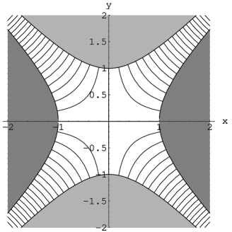
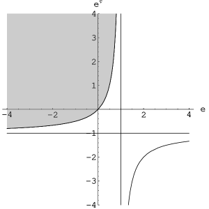
Figure 1: Left: Field lines of the quadrupolar electrostatic potential $V=e(x^{2}-y^{2})/2$. Right: phase diagram for elastic dipoles in the $(e_{0},e_{1})$ plane. The stable region is the domain in dark. Macroscopic strings get produced on the separatrix.

Let us start by considering a single direction $x$. The stability of the potential $V$ depends crucially on the sign of the determinant of $Q$,

$$D=\det(Q)=e_{1}-e_{0}-e_{0}e_{1}$$ (33)

If (i) $D>0$ and $e_{1}-e_{0}>-2$, the two eigenvalues are positive and the origin is a global minimum. If (ii) $D>0$ and $e_{1}-e_{0}<-2$ the two eigenvalues are negative and the origin is a global maximum. Finally, in the intermediate region (iii) where $D<0$, the two eigenvalues have opposite sign and the origin is a saddle point. This phase diagram is shown on Figure 1. Note that in the limit of zero string tension, the only stable region would have been $e_{1}>0,e_{0}<0$, corresponding to a stable electrostatic well for the two ends of the string. Thanks to the elastic binding energy, the stability domain extends partly into the two quarters $e_{0}e_{1}>0$. If we now add a second direction $y$, due to the tracelessness constraint on $h^{i}$, we are forced to choose opposite values $(-e_{0},-e_{1})$ for the gradient along $y$. It is evident from Figure 1 that there is no way to have the motion stable along the two directions at the same time. More generally, due to the convexity of the domain (i), there is no way to choose gradients $(e_{0}^{i},e_{1}^{i})$ along $n$ directions in the stable domain (i) while still maintaining the tracelessness constraint $\sum_{i=1,n}(e_{0}^{i},e_{1}^{i})=(0,0)$. This is consistent with the fact that the ground state of the string has a positive polarizability. One may ask whether choosing non-commuting electric gradients $(h_{0},h_{1})$ at the two ends may somehow stabilize the system, however investigation of the crossed configuration $\Phi_{0}=h_{0}(x^{2}-y^{2})/2,\Phi_{1}=h_{1}xy$ shows that this does not seem to be the case (see section 4.1.3 in the case of the open string). We will see in section 3.3 that stabilization can however be achieved by using a magnetic field, or by modulating the strength of the electric field.

In spite of the fact that this electrostatic configuration is globally unstable as it stands, there is still a rather interesting phenomenon that takes place at the critical line $D=0$: there the potential admits a degenerate valley, corresponding to stretched strings of arbitrary size $L$ in the direction $x$,

$$X=L(e_{0}\sigma-\pi)\ ,\quad\mbox{for}\quad e_{1}-e_{0}-e_{0}e_{1}=0\\$$ (34)

The physical origin of these states is clear: while the electrostatic potential decreases quadratically (when $e_{0}e_{1}>0$) like the square of the length, the tensive energy of the non-relativistic string grows like the square length as well, and there exists a critical value of the electric gradient for which the two forces cancel for any size. When this value is reached, the strings become macroscopic and extend to infinity, thereby discharging the condensator that created the electric field in the first place.

This phenomenon is very reminiscent of the critical electric field strength that appears in Born-Infeld electrodynamics, or equivalently for charged open strings in an electric field [33, 34]: the electric potential that pulls on the string ends grows with the length of the string $L$ as $EL$, while the tensive energy grows as $L/\alpha^{\prime}$. At the critical value $E_{c}=1/\alpha^{\prime}$, the two forces cancel and lead to strings of macroscopic size in the direction of the electric field, and small effective tension. If one attempts to go beyond $E_{c}$, the vacuum becomes unstable, tiny quantum strings get stretched to infinite distance very rapidly and discharge the condensator, thereby maintaining $E\leq E_{c}$. Such a regime has been used to construct the NCOS theory, a theory of non-commutative open strings decoupled from closed strings [30]. It would be very interesting to see if such a decoupling limit could be taken here as well, leading possibly to a theory of non-relativistic open strings only (see [35] for other attempts to define non-relativistic limits of closed strings). Another interesting question is whether and how these zero energy states can condense and backreact on the background (1). This may be especially tractable due to recent progress in open string field theory.

3.3 Elastic dipole in a Penning trap

While the purely electrostatic configuration of the previous section exhibited an interesting phase transition, it still suffers of a global instability, that may shed doubt on the existence of these macroscopic strings. We now switch on a magnetic field, and investigate whether the same mechanism that allowed to trap charged particles still succeeds in stabilizing the string. We therefore consider our dipole model in the electrostatic and magnetic fields

$$\Phi_{a}=\frac{1}{2}h_{a}\left(x^{2}+y^{2}-\frac{2}{1+b^{2}}z^{2}\right)\ ,\quad B=b~{}dx\wedge dy$$ (35)

Here, we have taken into account the modified harmonicity condition (6), which arises in dimension 3 and higher. According to our discussion in Section 2.1, this is the sole effect of $\alpha^{\prime}$ corrections (we have set $2\pi\alpha^{\prime}=1$). Along the third direction $z$, the dynamics is exactly the same as in the purely electrostatic case up to a redefinition of $(e_{0},e_{1})$, hence stability in this direction requires

$$\left(1+b^{2}+2e_{0}\right)\left(1+b^{2}-2e_{1}\right)-\left(1+b^{2}\right)^{2}>0$$ (36a)

$$\left(1+b^{2}\right)+e_{0}-e_{1}>0$$ (36b)

In the transverse directions, the magnetic field leads to a modified dispersion relation,

$$\begin{pmatrix}1-e_{0}-\omega^{2}&2ib\omega&-1&0\\ -2ib\omega&1-e_{0}-\omega^{2}&0&-1\\ -1&0&1+e_{1}-\omega^{2}&2ib\omega\\ 0&-1&-2ib\omega&1+e_{1}-\omega^{2}\end{pmatrix}\cdot\begin{pmatrix}x_{L}\\ y_{L}\\ x_{R}\\ y_{R}\end{pmatrix}(\omega)=0$$ (37)

At zero frequency, the effect of the magnetic field is nil, hence we still have production of macroscopic string states at the critical value of the electric gradients,

$$D=e_{1}-e_{0}-e_{0}e_{1}=0$$ (38)

However, crossing this line does not lead to an instability anymore, as we now show. The discriminant of the dispersion relation (i.e. the resultant $R$ of the polynomials $\det(Q)$ and $d\det(Q)/d\omega^{2}$) factorizes into

$$\begin{split}R=b^{4}\left[4+(e_{0}+e_{1})^{2}\right]^{2}&\left[4+\left(e_{0}+e_{1}\right)^{2}+8b^{2}(e_{0}-e_{1}-2)\right]^{2}\\ &\qquad\left[\left((1+b^{2})-e_{0}\right)\left((1+b^{2})+e_{1}\right)-1\right]\end{split}$$ (39)

When any of these factors vanishes, two roots $\omega^{2}$ of $\det(Q)$ collide, and may, or may not, leave the real axis. Experiment shows that the third factor gives rise to an accidental degeneracy but no instability, while the fourth does indeed lead to the disappearance of two positive real roots into the complex plane, and hence to a genuine instability. The crossing of (38) only leads to the appearance of one zero eigenvalue which becomes positive immediatly again. If we restrict to the line $e_{0}+e_{1}=0$ for simplicity, we therefore have the following transitions:

1. $e_{0}<0$: stable motion;

2. $e_{0}=0$: one zero mode, macroscopic strings are created;

3. $0<e_{0}<b^{2}$: only real roots, stable motion;

4. $e_{0}=b^{2}$: two eigenvalues become imaginary;

5. $b^{2}<e_{0}<2$: partially unstable motion;

6. $e_{0}=2$: one zero mode, macroscopic strings are created;

7. $2<e_{0}<2+b^{2}$: partially unstable motion;

8. $e_{0}=2+b^{2}$: two more eigenvalues become imaginary;

9. $e_{0}>2+b^{2}$: completely unstable motion;

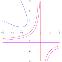
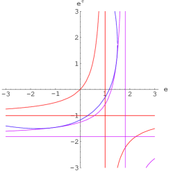
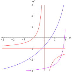
Figure 2: Phase diagram in the $(e_{0},e_{1})$ plane for strings in a quadrupolar potential with small (left), intermediate (center) or large (right) magnetic field; in purple, boudary of stability domain; in red, line of production of macroscopic strings; in blue, line of accidental degeneracy.

Here we have assumed that $b^{2}<2$. If not, the stable region includes up to $e_{0}=2$, hence displays creation of macroscopic strings twice. In addition, there is an additional degeneracy at $e_{0}=1-1/(4b^{2})$, which can occur either in the stable or unstable region. Examples of this phase diagram for several values of $b$ are given in Figure 2. To conclude, in the presence of a magnetic field, the stability region is enlarged to the upper left quadrant of the hyperbola:

$$\left(1+b^{2}-e_{0}\right)\left(1+b^{2}+e_{1}\right)-1>0,$$ (40a)

$$e_{0}<1+b^{2},$$ (40b)

The stable region therefore includes all of the first critical line for creation of macroscopic strings, and extends into the formerly unstable region up to

$$D\sim\frac{2-2e_{0}+e_{0}^{2}}{e_{0}-1}~{}b^{2}\qquad\mbox{for}\ \ b\ll 1$$ (41)

where the kinematic instability takes over. If $b^{2}>2$, part of the second critical line for creation of macroscopic strings is included into the kinematically stable region as well. It is now possible to combine the two conditions (36) and (40) to find a region with global stability in all $(x,y,z)$ directions.

3.4 Elastic dipole in a Paul trap

As we recalled in Sec 2.5, another standard way to trap ions in a quadrupolar electric field is to modulate the electric field periodically in time at a resonant frequency. Our aim in this section is to see to what extent the same mechanism can be used to trap charged elastic dipoles. Let us start by reviewing this mechanism in the point particle case. We thus consider a charged particle in a time-varying two-dimensional electric potential,

$$\Phi(x^{+})=\frac{1}{2}\left[h+fH\left(\frac{2\pi}{T}x^{+}\right)\right](x^{2}-y^{2})$$ (42)

where $H(t)$ is a periodic function of $t$ with period $2\pi$. After rescaling time, the equation of motion can be rewritten as

$$\ddot{X}+[\omega^{2}+\alpha^{2}H(t)]~{}X=0$$ (43)

where $(\omega^{2},\alpha^{2})=\pm(T/2\pi)^{2}(h,f)$ for $X=x,y$ respectively. For $H(t)=\cos t$, this is known as the Mathieu equation, whose solutions are well studied transcendental functions. The stability diagram of (43) however depends little on the details of the function $H(t)$, and can be studied much more easily in the case of a rectangular signal [37],

$$H(t)=1~{}\mbox{for}~{}t\in[2n\pi,(2n+1)\pi[,\ ,\quad H(t)=-1~{}\mbox{for}~{}t\in[(2n+1)\pi,(2n+2)\pi[\ .$$ (44)

Since $H(t)$ is periodic, the translation group must act by an element $\rho$ of $Sl(2,\mathbb{R})$ on a fundamental basis of solutions of the second order differential equation (43),

$$\begin{pmatrix}X_{1}\\ X_{2}\end{pmatrix}(t+2\pi)=\begin{pmatrix}a&b\\ c&d\end{pmatrix}\begin{pmatrix}X_{1}\\ X_{2}\end{pmatrix}(t)\ ,\quad ad-bc=1\ ,\quad W(X_{1},X_{2})=0$$ (45)

where $W(X_{1},X_{2})=X_{1}\partial_{t}X_{2}-X_{2}\partial_{t}X_{1}$ is the Wronskian, conserved in time. The eigenvalues of this $Sl(2,\mathbb{R})$ element can be written as $e^{\pm 2\pi i\mu}$ where the complex-valued Floquet exponent $\mu$ is computed from $\cos 2\pi\mu=(a+d)/2$. The motion is stable iff $\mu$ is real, i.e. $|\cos(2\pi\mu)|\leq 1$. For the rectangular signal (44), the matrix $\rho$ can be computed straightforwardly by matching $X$ and its derivative at $t=0$ and $t=\pi$. The Floquet exponent turns out to be determined by [37]

$$\cos(2\pi\mu)=\cos x_{1}\cos x_{2}-\frac{1}{2}\left(\frac{x_{1}}{x_{2}}+\frac{x_{2}}{x_{1}}\right)\sin x_{1}\sin x_{2}$$ (46)

where

$$x_{1}=\pi\sqrt{\omega^{2}+\alpha^{2}}\ ,\quad x_{2}=\pi\sqrt{\omega^{2}-\alpha^{2}}\ ,\quad$$ (47)

The domain of stability $|\cos(2\pi\mu)|\leq 1$ in the $(\omega^{2},\alpha^{2})$ plane is depicted in Figure 3. For a small ripple $\alpha\gg\omega$ and $\omega^{2}>0$, the motion is generically stable except when $\omega$ is integer or half-integer. At these values, the forcing is in resonance with the proper oscillation modes and an infinitesimal perturbation $\alpha$ is sufficient to destabilize the motion. This unstable region appears as a cusp on Figure 3, with boundaries well approximated at small $\alpha$ by

$$\omega^{2} = n^{2}+\left\{\begin{array}[]{c}-\frac{1}{4\,n^{2}}\alpha^{4}+\frac{\left(-9+n^{2}\,{\pi}^{2}\right)}{48\,n^{6}}{\alpha}^{8}\\ \frac{3}{4\,n^{2}}{\alpha}^{4}-\frac{\left(21+n^{2}\,{\pi}^{2}\right)}{48\,n^{6}}{\alpha}^{8}\end{array}\right\}+{\cal O}(\alpha^{12})\ ,\qquad n\in\mathbb{N}^{*}$$ (50)

$$\omega^{2} = \left(n+\frac{1}{2}\right)^{2}+\left\{\begin{array}[]{c}\frac{2}{\pi(2n+1)}\alpha^{2}+\frac{\pi^{2}(2n+1)^{2}-12}{(2n+1)^{4}\pi^{2}}\alpha^{4}\\ -\frac{2}{\pi(2n+1)}\alpha^{2}+\frac{\pi^{2}(2n+1)^{2}-12}{(2n+1)^{4}\pi^{2}}\alpha^{4}\end{array}\right\}+{\cal O}(\alpha^{6})\ ,\quad n\in\mathbb{N}$$ (53)

Conversely, an unstable motion at $\alpha=0$ can be made stable by switching on a small perturbation. Indeed, there appears to be a stable region extending in the $\omega^{2}<0$ domain above the line attaching at 0, well approximated by

$$\omega^{2}=-\frac{\pi^{2}}{12}\alpha^{4}+\frac{\pi^{6}}{1512}\alpha^{8}-\frac{107\pi^{10}}{9979200}\alpha^{12}+{\cal O}(\alpha^{16})$$ (54)

It is therefore possible to choose the period and amplitude of the forcing $(f,T)$ so that both $(\omega^{2},\alpha^{2})$ and $(-\omega^{2},-\alpha^{2})$ are in the stable region, hence the motion is stable in both directions $x$ and $y$.

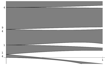
Figure 3: Left: stability diagram for an harmonic oscillator with frequency modulated by a rectangular signal, in the $(\omega^{2},\alpha^{2})$ plane. The stable region appears shaded, notice that it extends into the usually unstable regime $\omega^{2}<0$. Right: zoom on the region where $\alpha^{2}\ll 1$, axes are exchanged. Instabilities set in at half-integer $\omega$, even with an infinitesimal amplitude of modulation.

Let us now consider the case of an elastic dipole in a modulated quadrupole field. For simplicity, we assume that the same modulating frequency $T_{0}=T_{1}=T$ is applied on either end of the open strings, with opposite amplitudes $f_{0}=-f_{1}=f$. The equation of motion

$$\begin{pmatrix}\ddot{x}_{L}\\ \ddot{x}_{R}\end{pmatrix}+\frac{1}{\pi}\left[\begin{pmatrix}1-\pi p^{+}h_{0}&-1\\ -1&1+\pi p^{+}h_{1}\end{pmatrix}-p^{+}fH\left(\frac{2\pi}{T}x^{+}\right)\begin{pmatrix}1&\\ &1\end{pmatrix}\right]\begin{pmatrix}x_{L}\\ x_{R}\end{pmatrix}=0$$ (55)

can then be reduced to (43) for each of the proper directions of the constant matrix $Q$, with

$$\omega^{2}_{\pm} = \left(\frac{T}{2\pi p^{+}}\right)^{2}\frac{1}{\pi}\left(1+\frac{e_{1}-e_{0}}{2}\pm\sqrt{1+\frac{(e_{0}+e_{1})^{2}}{4}}\right)$$ (56)

$$\alpha^{2} = \left(\frac{T}{2\pi p^{+}}\right)^{2}f$$ (57)

where the two signs correspond to the two modes of $Q$ in the $x$ direction. In the limit of small tension, the two eigenmodes $\omega^{2}_{\pm}$ become

$$\omega_{+}=\left(\frac{T}{2\pi p^{+}}\right)^{2}\frac{1}{\pi}\left(-e_{0}+1+{\cal O}(1/h)\right)\ ,\quad\omega_{-}=\left(\frac{T}{2\pi p^{+}}\right)^{2}\frac{1}{\pi}\left(e_{1}+1+{\cal O}(1/h)\right)$$ (58)

The eigenmodes in the $x$ and $y$ directions are therefore not opposite anymore but shifted together upward. Nevertheless it is clear that for small enough tension one will still be able to choose the perturbation $f$ such that both directions are stabilized.

3.5 Elastic dipole in an adiabatically varying electric field

After having discussed the motion of an elastic dipole in a resonant quadrupolar case, we now consider a dipole in a time-dependent quadrupolar potential $\Phi_{a}(x^{+})=h_{a}(x^{+})(x^{2}-y^{2})/2$, which we assume to vary adiabatically between two non-zero asymptotic values $h_{a}(\pm\infty)$. In the particular case $h_{0}(x^{+})=-h_{1}(x^{+})=h(x^{+})$, the mass matrix $Q(x^{+})$ can be diagonalized independently of time, yielding two decoupled harmonic oscillators with time-dependent frequency,

$$\ddot{x}_{\pm}+\omega^{2}_{\pm}(\tau)x_{\pm}=0$$ (59)

with $\omega^{2}_{\pm}=p^{+}h(x^{+})\pm 1$, $x_{\pm}=x_{L}\mp x_{R}$. This problem can be solved for an arbitrary profile $h(x^{+})$ by separating the modulus and phase of, say, $x_{\pm}=s_{\pm}e^{i\gamma_{\pm}}$. The imaginary part of the equation relates the rate of phase variation to the modulus through $s_{\pm}^{2}\dot{\gamma}_{\pm}=\text{cte}$ which can be set to 1. The real part gives a non-linear differential equation for the modulus,

$$\ddot{s}_{\pm}+\omega^{2}_{\pm}(\tau)s_{\pm}=\frac{1}{s_{\pm}^{3}}$$ (60)

The complete quantum mechanical S-matrix can then be found from the knowledge of $s_{\pm}$ at late times, where (60) reduces to the equation of motion deduced from the Hamiltonian of conformal quantum mechanics [39]. This result does not rely on any adiabaticity assumption, although determining $s_{\pm}(+\infty)$ may not be feasible analytically.

In the general case however, the proper directions of $Q$ change with time, and it no longer helps to diagonalize the Hamiltonian. Instead, one may eliminate $x_{L}$ (say) and obtain a $4^{\text{th}}$-order differential equation for $x=x_{R}$,

$$\pi x^{(4)}+(\text{tr }Q)\ddot{x}+\det Q=0$$ (61)

where we recall that $\text{tr }Q=2+e_{1}-e_{0}$ and $\det Q=e_{1}-e_{0}-e_{1}e_{0}$. It is not possible anymore to separate the phase and modulus of $x=se^{i\gamma}$ in general (although the imaginary part of (61) can be integrated once after multiplying by the integrating factor $s(\tau)$), however the problem can be solved in the adiabatic regime $\dot{h}_{a}\ll h^{3/2}$. Following the standard WKB method, we rescale $t\to t/\epsilon$ and $\gamma\to\gamma/\epsilon$. At leading order, (61) identifies the rate of phase variation with one of the instantaneous proper frequencies,

$$\dot{\gamma}=\omega(\tau)=\pm\sqrt{\frac{\text{tr }Q}{2\pi}\pm\frac{1}{\pi}\sqrt{1+\frac{1}{4}(e_{0}+e_{1})^{2}}}\ ,$$ (62)

hence $\gamma(\tau)=\int_{0}^{\tau}\omega(\tau^{\prime})d\tau^{\prime}$, while the amplitude is given at next-to-leading order by

$$s(\tau)=\frac{s(0)}{\left({\cal A}(\tau)\right)^{1/2}}\exp\int_{0}^{\tau}\frac{ip^{+}(\dot{e}_{1}(\tau^{\prime})-\dot{e}_{0}(\tau^{\prime}))\omega(\tau^{\prime})}{\pi{\cal A}(\tau^{\prime})}d\tau^{\prime}$$ (63)

where

$${\cal A}(\tau)=2\left(\frac{i}{\pi}(e_{1}(\tau)-e_{0}(\tau)+2)\omega(\tau)-2i\omega(\tau)^{3}\right)$$ (64)

and $\omega$ denotes one of the branches of (62). The approximation remains valid as long as all eigenvalues stay separate from each other. In particular it breaks down at the line of production of macroscopic dipoles where two eigenvalues collide and leave the real axis. It would also break down if the electric gradient $h_{a}$ was switched off at $\pm\infty$, except in the proper direction $x^{+}$ which remains confined due to the string tension.

4 Open strings in a null quadrupolar electric field

We now proceed with the first quantization of a string in a quadrupolar electrostatic potential $\Phi_{a}={h_{a}}_{ij}x^{i}x^{j}/2$, where ${h_{a}}_{ij}$ are constant traceless matrices, independent of $x^{+}$. For now, we do not assume any particular commutation relation between $h_{0}$ and $h_{1}$.

4.1 First quantization in a constant quadratic potential

When decomposing $X$ in left and right movers (10), the boundary condition (14) translates into the system of linear equations

$$\dot{f}(\tau)-\dot{g}(\tau) +p^{+}h_{0}\bigl{(}f(\tau)+g(\tau)\bigr{)}+B\bigl{(}\dot{f}(\tau)+\dot{g}(\tau)\bigr{)}=0$$ (65)

$$T^{2}\dot{f}(\tau)-\dot{g}(\tau) +p^{+}h_{1}\bigl{(}T^{2}f(\tau)+g(\tau)\bigr{)}+B\bigl{(}T^{2}\dot{f}(\tau)+\dot{g}(\tau)\bigr{)}=0$$

where $T^{2}$ denotes the translation operator, $T^{2}f(\tau)=f(\tau+2\pi)$. In order to avoid cluttering, we have absorbed a factor $p^{+}$ into the gradients $h_{a}$, and omitted the $d\times d$ indices. Such non-local differential problems have been studied in the mathematical literature under the name of linear differential difference equation of neutral type [41]. They are in contrast to the case of closed strings in gravitational waves, where the classical dynamics reduces to an ordinary differential equation for each mode of the Fourier expansion of the periodic coordinates $X(\sigma)$. They can nevertheless be solved rather straightforwardly using Fourier (or Laplace) analysis.

4.1.1 Neutral string

Before proceeding to the general case, let us first discuss the neutral case of an open string starting and ending on the same brane $h_{0}=h_{1}:=h$. Taking the difference of the two equations above, we get

$$(T^{2}-1)(\dot{f}+p^{+}hf+B\dot{f})=0$$ (66)

Hence $\dot{f}(\tau)+p^{+}hf(\tau)+B\dot{f}$ has to be a periodic function of $\tau$, with the Fourier series expansion (we assume $[e,B]=0$),

$$\dot{f}(\tau)+\frac{e}{\pi}f(\tau)+B\dot{f}(\tau)=a_{0}+\sum_{n\neq 0}\left((1+B)+\frac{i}{n\pi}e\right){\cal M}_{n}a_{n}e^{-in\tau}=\dot{g}(\tau)-\frac{e}{\pi}g(\tau)-B\dot{g}(\tau).$$ (67)

We chose a somewhat awkward normalisation of the $a_{n}$’s in order to get the correct commutation relations at the end. (67) can be easily integrated to yield the normal mode expansion:

$$\begin{split}X(\tau,\sigma)=&{\cal M}^{u}_{+}\frac{\pi(1-B)}{e}e^{\frac{e}{\pi(1-B)}(\tau-\sigma)}a_{+}-{\cal M}^{u}_{-}\frac{\pi(1+B)}{e}e^{-\frac{e}{\pi(1+B)}(\tau+\sigma)}a_{-}\\ &+\sum_{n\neq 0}{\cal M}_{n}\frac{i}{n}\left[e^{-in(\tau+\sigma)}+\frac{in\pi(1+B)-e}{in\pi(1-B)+e}e^{-in(\tau-\sigma)}\right]a_{n}\end{split}$$ (68)

where $d\times d$ matrices are still understood. The normalisation coefficients are given in Appendix C. The expansion therefore remains integer modded as in the $e=0$ case, with the apparition of exponentially varying zero-modes $(a_{+},a_{-})$. With the normalisation chosen, we have the standard commutation relations:

$$[a^{i}_{n},a^{j}_{m}]=n\delta^{ij}\delta_{n,-m}\qquad[a^{i}_{+},a^{j}_{-}]=i\frac{1}{\pi}e^{ij}$$ (69)

The Hamiltonian (25) can be easily computed:

$$p^{+}{\cal H}_{lc}=a_{+}a_{-}+\sum_{n=1}^{\infty}a^{\dagger}_{n}a_{n}-\frac{D}{24}$$ (70)

4.1.2 Charged string

Let us now come back to the general case with $e_{0}\neq e_{1}$, in the absence of a magnetic field for simplicity. Decomposing $f$ and $g$ into their Fourier modes, Equation (65) becomes a linear system

$$\begin{pmatrix}-i\omega+\frac{e_{0}}{\pi}&i\omega+\frac{e_{0}}{\pi}\\ (-i\omega+\frac{e_{1}}{\pi})e^{-2i\pi\omega}&i\omega+\frac{e_{1}}{\pi}\end{pmatrix}\begin{pmatrix}\hat{f}(\omega)\\ \hat{g}(\omega)\end{pmatrix}=0$$ (71)

The compatibility of this linear system puts a quantization condition on the energies $\omega$, which can be rewritten as the secular equation

$$\det\left[\left((\pi\omega)^{2}+e_{1}e_{0}\right)\sin(\pi\omega)-(e_{1}-e_{0})\pi\omega\cos(\pi\omega)\right]=0$$ (72)

Now let us assume that $e_{0}$ and $e_{1}$ commute (the case where they do not will be briefly considered in section 4.1.3). The two matrices can then be diagonalized simultaneously and we can restrict ourselves to a potential of the form $\frac{1}{2}(x^{2}-y^{2})$ where $x$ and $y$ are two spatial directions. The problem thus decouples into two one-dimensional problems related by inverting $(e_{0},e_{1})\to(-e_{0},-e_{1})$. The dispersion relation (72) thus reads

$$e^{2\pi i\omega}=\frac{i\pi\omega+e_{0}}{i\pi\omega-e_{0}}\frac{i\pi\omega-e_{1}}{i\pi\omega+e_{1}}$$ (73a)

or equivalently

$$\tan(\pi\omega)=\frac{(e_{1}-e_{0})\pi\omega}{(\pi\omega)^{2}+e_{0}e_{1}}$$ (73b)

To find solutions of (73a) graphically, one has to look at the intersection points of the “Lorentzian curve” on the rhs with the $\tan$ curve on the lhs . The secular equation selects one real eigenmode $\omega_{n}$ in any interval $[n\pi,(n+1)\pi[$, $n\in\mathbb{N}^{*}$, with wave function

$$X_{n}(\tau,\sigma)={\cal N}_{n}\frac{i}{\omega_{n}}\left(e^{-i\omega_{n}(\tau+\sigma)}+\frac{i\pi\omega_{n}-e_{0}}{i\pi\omega_{n}+e_{0}}e^{-i\omega_{n}(\tau-\sigma)}\right)a_{n}+h.c.\qquad n>0$$ (74)

where the normalization factor ${\cal N}_{n}$, given in Appendix C, ensures that the commutators are indeed $[a_{n},a_{m}^{\dagger}]=\omega_{n}\delta_{n,m}$.

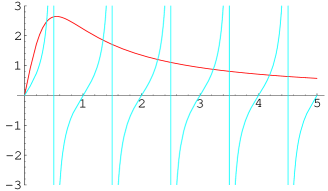
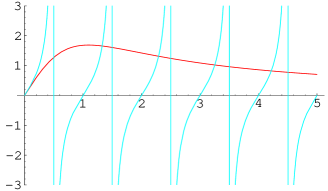
Figure 4: Graphical solution of the open string dispersion relation for a one-dimensional harmonic potential. Left: $D>0$, $e_{1}-e_{0}>-2$, all roots are real. Right: $D<0$, $e_{1}-e_{0}>-2$, two roots have collided at $\omega=0$ and left into the complex plane.

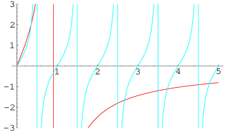
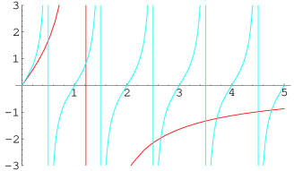
Figure 5: Graphical solution of the open string dispersion relation for a one-dimensional harmonic potential. Left: $D<0$, $e_{1}-e_{0}<-2$, the root in the interval $[0,1]$ corresponds to the first excited level. Right: $D>0$, $e_{1}-e_{0}<-2$, two more roots have collided at $\omega=0$ and left into the complex plane.

The situation for the first segment $[0,1[$ is more subtle however (see Figures 4 and 5):

• $D=e_{1}-e_{0}-e_{0}e_{1}>0$ and $e_{1}-e_{0}>-2$

  There is a single real root $\omega_{0}\neq 0$ in $]0,1[$. As shown in Appendix A, all the roots are then real and the motion is stable. The wave function $X_{0}$ is the same as (74) with $n=0$.

• $D=0$ and $e_{1}-e_{0}>-2$

  As $D$ approaches 0, the real root $\omega_{0}$ collides with its opposite $-\omega_{0}$ , leading to a pair of canonically conjugate modes with vanishing frequency. Their wave function can be obtained from the $\omega_{n}\to 0$ limit of (74), and reads

  $$X_{c}(\tau,\sigma)={\cal N}_{0}^{c}(1-\frac{e_{0}}{\pi}\sigma)(x_{0}+p_{0}\tau)$$ (75)

  where again the normalization (see Appendix C) gives the canonical brackets, $[x_{0},p_{0}]~{}=~{}i$. Those are exactly the macroscopic strings described in the previous section, occurring at a critical value of the gradient of the electric field. For small deviation away from the critical gradient, their energy is given by

  $$\omega_{0}=\sqrt{\frac{3(1-e_{0})}{\pi^{2}(2-3e_{0}+e_{0}^{2})}D}$$ (76)

• $D<0$ (note that the line $e_{1}-e_{0}=-2$ is contained in this domain)

  As $D$ becomes negative, these two roots leave the real axis and become purely imaginary, $\omega_{0}^{\pm}=\pm ik_{0}$. This corresponds to unstable modes, with wave function

  $$X_{\pm}(\tau,\sigma)={\cal N}^{u}\frac{1}{k_{0}}\left(e^{\pm k_{0}(\tau+\sigma)}+\frac{\mp\pi k_{0}-e_{0}}{\mp\pi k_{0}+e_{0}}e^{\pm k_{0}(\tau-\sigma)}\right)a_{\pm}\ ,\quad[a_{+},a_{-}]=ik_{0}$$ (77)

• $D>0$ and $e_{1}-e_{0}<-2$

  When crossing the $D=0$ curve in the region $e_{1}-e_{0}<-2$, the two roots $\pm\omega_{1}$ collide, hence two new macroscopic modes appear and then become unstable. They behave like unstable modes described above in the case where $D<0$.

Altogether, we have thus found exactly the same phase diagram as in our dipole model, implying that the afore-mentioned instabilities have indeed a low-energy origin. Having found the normal modes, we can now carry out a standard mode expansion, focusing on the region of the stability diagram where $e_{1}-e_{0}>-2$,

$$X(\tau,\sigma)=\sum_{n=1}^{\infty}X_{n}+\begin{cases}D>0:&X_{0}\\ D=0:&X_{c}\\ D<0:&X_{+}+X_{-}\end{cases}$$ (78a)

with canonical commutation relations,

$$[a_{n},a^{\dagger}_{m}]~{}=~{}\omega_{n}\delta_{n,m},\qquad[x_{0},p_{0}]~{}=~{}i,\qquad[a_{+},a_{-}]~{}=~{}ik_{0}.$$ (79)

The contribution of the $X$ coordinate to the light-cone Hamiltonian is easily evaluated in terms of these variables, and reads

$$p^{+}{\cal H}_{X}=\sum_{n=1}^{\infty}a^{\dagger}_{n}a_{n}+\left\{\begin{matrix}D>0:&a^{\dagger}_{0}a_{0}\\ D=0:&p_{0}^{2}\\ D<0:&a_{+}a_{-}\end{matrix}\right\}+E_{X}$$ (80)

The vacuum energy $E_{X}$ has been evaluated using contour integral methods in [43]. The contribution of the boson $Y$ can be obtained from (80) by simply reversing the sign of $(e_{0},e_{1})$ (note that $D$ is not invariant under this operation).

4.1.3 Non commuting electric gradients

The dispersion relation (72) cannot be solved as easily as before, but we can examine the following crossed configuration:

$$h_{0}=h\begin{pmatrix}1&\\ &-1\end{pmatrix}\ ,\quad h_{1}=h^{\prime}\begin{pmatrix}&1\\ 1&\end{pmatrix}$$ (81)

The secular equation still factorizes into

$$\tan(\pi\omega)=\pm\frac{\pi\omega~{}\sqrt{e^{2}+e^{{}^{\prime}2}}}{\sqrt{(\pi\omega)^{4}+e^{2}e^{{}^{\prime}2}}}$$ (82)

The structure of roots is similar to the commuting case, except that the critical line is now at $D=e^{2}+e^{{}^{\prime}2}-e^{2}e^{\prime 2}=0$, at which the slope at $\omega=0$ of the lhs of (82) coincide the rhs (with the $+$ sign). As before, for all $n>0$ there exists a real root in $[n,(n+1)[$. For the branch with $-$ sign, the slope at $\omega=0$ will always be negative and there will never be an additional zero in the interval $[0,1[$. However, there are always two complex roots $\hat{\omega}_{0}=\pm i\tilde{k}_{0}$ , that is to say, two unstable modes $\hat{a}_{+}$ and $\hat{a}_{-}$ (we use a $\hat{}$ for oscillators of the minus branch, nothing for the plus branch). For the positive branch, the situation is comparable to the commutative case. If $D>0$, there also exists a real root $\omega_{0}$ in $[0,1[$. As $D\to 0$, this roots collides with its opposite and leaves the real axis. For $D<0$, it becomes a pair of complex conjugate roots $\omega_{0}=\pm ik_{0}$ corresponding to the instability described in the previous section. At $D=0$, we have macroscopic strings with arbitrary length,

$$\begin{pmatrix}X_{c}\\ Y_{c}\end{pmatrix}=\sqrt{\frac{3(e^{2}-\pi)}{2e^{3}\pi^{2}}}(x_{0}+p_{0}t)\begin{pmatrix}\frac{1-\frac{e}{\pi}\sigma}{\sqrt{e-1}}\\ \frac{1+\frac{e}{\pi}\sigma}{\sqrt{e+1}}\end{pmatrix}$$ (83)

and fixed angle $X_{c}/Y_{c}=\sqrt{(e+1)/(e-1)}$. The Hamiltonian can be evaluated on this configuration and reads

$$p^{+}{\cal H}=\sum_{n=1}^{\infty}a^{\dagger}_{n}a_{n}+\sum_{n=1}^{\infty}\hat{a}^{\dagger}_{n}\hat{a}_{n}+\left\{\begin{matrix}D>0:&a^{\dagger}_{0}a_{0}\\ D=0:&p_{0}^{2}\\ D<0:&a_{+}a_{-}\end{matrix}\right\}+\hat{a}_{+}\hat{a}_{-}+E_{vac}$$ (84)

Non-commuting electric gradients therefore lift part of the degeneracy of the commuting case, but do not prevent the kinematic instability to take place.

4.2 Open string in a Penning trap

While the sign of the quadrupolar potential was chosen so that the direction $z$ was confining, the transverse $(x,y)$ plane corresponds to unstable directions of the electric field. As we discussed in 3.3, this can be stabilized by adding a constant magnetic field in the $(x,y)$ plane. For simplicity we assume that $e$ and $B$ commute. The linear system (71) becomes

$$\begin{pmatrix}-(1+B)i\pi\omega+e_{0}&(1-B)i\pi\omega+e_{0}\\ (-(1+B)i\pi\omega+e_{1})e^{-2i\pi\omega}&(1-B)i\pi\omega+e_{1}\end{pmatrix}\begin{pmatrix}\hat{f}(\omega)\\ \hat{g}(\omega)\end{pmatrix}=0$$ (85)

The dispersion relation splits into two branches,

$$\tan(\pi\omega)=\frac{\pi\omega(e_{1}-e_{0})}{(1+b^{2})(\pi\omega)^{2}\pm b(e_{0}+e_{1})(\pi\omega)+e_{0}e_{1}}$$ (86)

where the two signs correspond to the left and right-handed circular polarizations. Reversing $\omega$ exchanges the two branches, so that the two polarizations are canonically conjugate; we can therefore focus on the upper sign only. As before, a phase transition occurs when the tangents of the two curves on either side of (86) become equals. As $b$ couples only at higher order in $\omega$, the transition line remains unaffected at $D=e_{1}-e_{0}-e_{0}e_{1}=0$. In contrast to (73a) however, only a single root collides with $\omega=0$, as can be seen by expanding the dispersion relation at $\omega=0$ close to the transition line $D\to 0$,

$$\frac{(e_{0}-1)D}{e_{0}^{2}}(\pi\omega)+\frac{(e_{0}-2)b}{e_{0}}(\pi\omega)^{2}+\frac{(1-3b^{2})(3-3e_{0}+e_{0}^{2})}{3e_{0}^{2}}(\pi\omega)^{3}+{\cal O}(\omega^{4})=0$$ (87)

When $D\to 0$, one of the roots collides with $0$, but simply crosses it as $D$ changes sign. There is therefore no instability associated with the phase transition at $D=0$, instead a creation of static macroscopic strings takes place as in the absence of a magnetic field. This is not surprising, since the effect of the magnetic field should only be felt in dynamical situations. On the other hand, an instability does take place as one goes further away from $D=0$: indeed, by looking at the next term in the expansion (87), one sees that the two roots $\omega_{0}$ and $\omega_{1}$ collide and leave the real axis at a critical value

$$b_{c}^{2}=\frac{4(e_{0}-1)(3-3e_{0}+e_{0}^{2})}{3e_{0}^{2}(e_{0}-2)^{2}}D\ ,\quad D\ll 1$$ (88)

This is qualitatively the same as in our dipole model (41). As in the case of the dipole model in section 3.3, the stability region is enlarged so as to include a part of the macroscopic string creation line and to allow global stability region as regards $x$ and $y$ coordinates. Unfortunately, the precise critical line at finite $D$ does not seem to be computable explicitely. At any rate, this demonstrates that the same set-up that allowed to stabilize elastic dipoles in a 3D quadrupolar potential also works for the full open string.

4.3 One-loop amplitude and open-closed duality

Just as gravitational plane waves exhibit no particle production nor vacuum polarization, the same is true for electromagnetic plane waves. A simple way to see this is to return to the Coleman formula for the one-loop vacuum free energy, written in light-cone variables,

$$A=\frac{1}{2}V_{+-}\sum_{i}\int_{0}^{\infty}\frac{dt}{t}\int\frac{dp^{+}dp^{-}}{(2\pi)^{2}}\exp\left(i(p^{+}p^{-}+m_{i}^{2})t\right)$$ (89)

where we included the transverse momenta and string excitation levels in the label $i$, and denoted by $V_{+-}$ the volume of light-cone directions. The integral over $p^{-}$ enforces a delta function $\delta(tp^{+})$, which implies that only $p^{+}=0$ states contribute to the vacuum energy: but these states are insensitive to the presence of the null electromagnetic field, hence the vacuum energy reduces to that of flat space. Equivalently, in order to form a loop of open strings, one should make the worldsheet time $\tau$ periodic, but this is incompatible with the light-cone gauge $X^{+}=x_{0}^{+}+p^{+}\tau$ unless $p^{+}=0$.

On the other hand, it is well known that a non-trivial contribution to the vacuum energy is obtained when the light-cone coordinate $X^{+}$ is compact of radius $R$. Indeed, the integral over $p^{-}$ in (89) is turned into a discrete sum on integers $p^{-}=n/R$, or after Poisson resummation into a periodic delta distribution with support at $p^{+}=wR/t$, $w\in\mathbb{Z}$. One-loop vacuum energy with a loop modulus of $2\pi t$ writes

$$A_{op}=\frac{1}{2}V_{+-}\sum_{w=-\infty}^{\infty}\int_{0}^{\infty}\frac{dt}{t^{2}}\left.\mbox{Tr}\exp(i2\pi m^{2}t)\right\rvert_{p^{+}=Rw/t}$$ (90)

The quantization of $p^{+}$ is now in agreement with the fact that $X^{+}$ should be a periodic function of $\tau$ of period $2\pi t$, modulo the identification $X^{+}\sim X^{+}+2\pi wR$. For open strings, $m^{2}=p^{+}{\cal H}_{op}$ and after a Wick rotation, one obtains

$$\begin{split}A_{op}&=-\frac{i}{2}V_{+-}\sum_{w=-\infty}^{\infty}\int_{0}^{\infty}\frac{dt}{t^{2}}\left.\mbox{Tr}\exp\left(-2\pi p^{+}{\cal H}_{op}t\right)\right\rvert_{p^{+}=Rw/t}\\ &=-\frac{i}{2}V_{+-}\sum_{w=-\infty}^{\infty}\int_{0}^{\infty}\frac{dt}{t^{2}}Z_{op}(t)\end{split}$$ (91)

As usual, the open string vacuum amplitude should be reexpressible in the closed string channel as the propagator of closed strings between two boundary states describing the two D-branes with the electromagnetic flux on them. Since our D-branes have Neumann boundary condition along the light-cone coordinate $X^{+}$, it is not possible to use the standard light-cone gauge to quantize the closed strings. Instead, one may use $X^{+}=wR\sigma$, which follows directly from the open-string light-cone gauge $X^{+}=p^{+}\tau$ after exchanging and rescaling the worldsheet coordinates, $\tau\to t\sigma$. The integer $w$ is now interpreted as the winding number of the closed string around the compact coordinate $X^{+}$. The closed string amplitude therefore reads

$$A_{cl}=\sum_{i}\langle B_{1}\rvert\frac{1}{p^{+}p^{-}+m_{i}^{2}}\lvert B_{0}\rangle$$ (92)

where we used the fact that the boundary states $B_{0}$ and $B_{1}$ are annihilated by $p^{+}$ and $p^{-}$. For closed strings propagation with Schwinger time $\pi\hat{t}$

$$\begin{split}A_{cl}&=\sum_{w=-\infty}^{\infty}\int_{0}^{\infty}d\hat{t}\langle B_{1}(w)|e^{-\pi\hat{t}H_{cl}}\lvert B_{0}(w)\rangle\\ &=\sum_{w=-\infty}^{\infty}\int_{0}^{\infty}d\hat{t}~{}V_{+-}~{}Z_{cl}(\hat{t})\end{split}$$ (93)

The equality between (90) and (93) for D-branes in flat space now follows from the usual modular properties of open/closed string partition functions.

We now return to the case of charged open strings in a constant quadrupolar electromagnetic wave, $\Phi_{a}=(h_{a})_{ij}x^{i}x^{j}$ and compute the one-loop vacuum energy in the case where the light-cone coordinate $X^{+}$ is compact. Then, boundary conditions for open and closed strings involve parameter $e$ and $\hat{e}$ which are

$$e_{a}=\pi p^{+}h_{a}=\pi wRh_{a}/t\ ,\qquad\hat{e}_{a}=\pi wRh_{a}=\pi p^{+}h_{a}t,$$ (94)

and thus obey the duality relation $\hat{e}_{a}=e_{a}t$ (in fact, there is a $i$ coming from the Wick rotation, see (165)). Starting with the open string channel, the contribution of the coordinate $X$ with $e_{0}^{X}=e_{0}$ and $e_{1}^{X}=e_{1}$ on a cylinder of modulus $q=e^{-2\pi t}$ is given, with due care paid to the zero-mode, by

$$Z_{op}(t,e_{0},e_{1})=q^{E_{X}}\prod_{n=1}^{\infty}\left(1-q^{\omega_{n}}\right)^{-1}\times\begin{cases}\left(1-q^{\omega_{0}}\right)^{-1}&\text{if }D>0\\ \frac{1}{2t}\sqrt{\frac{(2-3e_{0}+e_{0}^{2})}{3(1-e_{0})D}}&\text{if }D\to 0\\ \left(1-q^{ik_{0}}\right)^{-1}&\text{if }D<0\end{cases}$$ (95)

In the zero field limit, one retrieves the correct behaviour

$$Z_{op}(t,e_{0},e_{1})\sim\frac{1}{\sqrt{e_{0}-e_{1}}t~{}\eta(t)}\sim\frac{1}{\sqrt{ht}~{}\eta(t)}\sim\frac{V}{\sqrt{t}~{}\eta(t)}$$ (96)

where V is the volume accessible to 0-modes and $\eta(t)=q^{\frac{1}{24}}\prod_{n=1}^{\infty}\left(1-q^{n}\right)$ is the Dedekind eta function. The one-loop open string amplitude is obtained by putting together the contributions of the $x$ and $y$ directions as well as the remaining 22 transverse coordinates $x^{i}$, and reads

$$A_{op}=-\frac{i}{2}V_{+-}\sum_{w=-\infty}^{\infty}\int_{0}^{+\infty}\frac{dt}{t^{2}}\,{\cal V}_{22}(4\pi^{2}t\eta^{2}(t))^{-11}Z_{op}(t,e_{0},e_{1})Z_{op}(t,-e_{0},-e_{1})$$ (97)

where ${\cal V}_{22}$ is the volume of the 22 free transverse directions. For $D<0$, the partition function picks an imaginary part, due to the unstable mode $k_{0}$. It would be interesting to extract the production rate of macroscopic strings, in analogy with the stringy computation of Schwinger pair production in [40].

Now we turn to the closed string channel. As explained above, it is convenient to use a non-standard light-cone gauge $X^{+}(\tau,\sigma)=Rw\sigma$, compatible with the Neumann boundary condition on $X^{+}$. Focusing on a single transverse boson $X$, the boundary condition (14) at $\sigma=0$ becomes a condition at one cap $\tau=0$ of the cylinder,

$$\partial_{\tau}X+\frac{\hat{e}}{\pi}X=0\quad\mbox{at}\ \tau=0$$ (98)

with $\hat{e}/\pi$ given in (94). The coordinate $X$ still satisfies the free field equation $(\partial_{\tau}^{2}-\partial_{\sigma}^{2})X=0$ in the bulk, and can be expanded in the usual free closed string modes,

$$X_{cl}=x_{0}+p_{0}\tau+i\sum_{n\neq 0}\frac{1}{n}\left(\alpha_{n}e^{-in(\tau+\sigma)}+\tilde{\alpha}_{n}e^{-in(\tau-\sigma)}\right)$$ (99)

The condition (98) can now be written as a condition on a boundary state $|B(\hat{e})\rangle$ in the closed string Hilbert space,

$$\left[\left(1+\frac{i\hat{e}}{\pi n}\right)\alpha_{n}+\left(1-\frac{i\hat{e}}{\pi n}\right)\tilde{\alpha}_{-n}\right]\left|B(\hat{e})\right\rangle=0$$ (100a)

$$\left(p_{0}+\frac{\hat{e}}{\pi}x_{0}\right)\left|B(\hat{e})\right\rangle=0$$ (100b)

which can be solved as usual by coherent state techniques,

$$|B(\hat{e})\rangle={\cal N}(\hat{e})\,e^{i\frac{\pi p_{0}^{2}}{2\hat{e}}}\exp\left(\sum_{n=1}^{\infty}-\frac{1}{n}\frac{i\pi n+\hat{e}}{i\pi n-\hat{e}}\alpha_{-n}\tilde{\alpha}_{-n}\right)|0,\tilde{0}\rangle$$ (101)

where

$${\cal N}(\hat{e})=\frac{1}{\sqrt{2\sqrt{2}\sinh(\hat{e})}}.$$ (171)

is fixed by open-closed duality as explained in Appendix B. Here we used a momentum representation to solve the zero-mode constraint (100b). The contribution of the coordinate $X$ with $\hat{e}_{0}^{X}=\hat{e}_{0}$ and $\hat{e}_{1}^{X}=\hat{e}_{1}$ to the one-loop amplitude in the closed string channel is now simply obtained as

$$Z_{cl}=\int dp_{0}\langle B(\hat{e}_{1})\rvert e^{-\pi\hat{t}p^{+}{\cal H}^{cl}}\lvert B(\hat{e}_{0})\rangle$$ (102)

where we included a summation over the closed string zero-mode $p_{0}$ along the direction $x$. The free closed string Hamiltonian reads as usual

$$p^{+}{\cal H}^{cl}=\frac{1}{2}p_{0}^{2}+\sum_{n=1}^{\infty}(\alpha_{-n}\alpha_{n}+\tilde{\alpha}_{-n}\tilde{\alpha}_{n})-\frac{1}{24}$$ (103)

The matrix element (102) can now be evaluated using the identity

$$\left<0,\tilde{0}\right|e^{\lambda_{1}^{*}\alpha\tilde{\alpha}}e^{-\pi\hat{t}(\alpha^{\dagger}\alpha+\tilde{\alpha}^{\dagger}\tilde{\alpha})}e^{\lambda_{0}\alpha^{\dagger}\tilde{\alpha}^{\dagger}}\left|0,\tilde{0}\right>=\frac{1}{1-\lambda_{1}^{*}\lambda_{0}e^{-2\pi\hat{t}}}$$ (104)

where we assumed the commutation relations $[\alpha,\alpha^{\dagger}]=[\tilde{\alpha},\tilde{\alpha}^{\dagger}]=1$. The integral on the zero-mode $p_{0}$ is Gaussian. Altogether, we obtain, keeping in mind that the commutation relations for the $\alpha_{n}$’s and the $\tilde{\alpha}_{n}$’s are $[\alpha_{n},\alpha^{\dagger}_{n}]=n$ and $[\tilde{\alpha}_{n},\tilde{\alpha}^{\dagger}_{n}]=n$ :

$$Z_{cl}(\hat{t},\hat{e}_{0},\hat{e}_{1})={\cal N}(\hat{e}_{0}){\cal N}(\hat{e}_{1})\sqrt{\frac{2}{\hat{t}+i\left(\frac{1}{\hat{e}_{1}}-\frac{1}{\hat{e}_{0}}\right)}}\hat{q}^{-\frac{1}{24}}\prod_{n=1}^{\infty}\left(1-\frac{i\pi n+\hat{e}_{0}}{i\pi n-\hat{e}_{0}}\frac{i\pi n-\hat{e}_{1}}{i\pi n+\hat{e}_{1}}\hat{q}^{n}\right)^{-1}$$ (105)

where $\hat{q}=e^{-2\pi\hat{t}}$. In the zero field limit, one obtains correctly

$$Z_{cl}(\hat{t},\hat{e}_{0},\hat{e}_{1})\sim\frac{1}{\sqrt{\hat{e}_{0}-\hat{e}_{1}}\eta(\hat{t})}\sim\frac{1}{\sqrt{h}~{}\eta(\hat{t})}\sim\frac{V}{\eta(\hat{t})}$$ (106)

One therefore obtains the one-loop amplitude in the closed string channel,

$$A_{cl}=\sum_{w=-\infty}^{\infty}\int_{0}^{+\infty}d\hat{t}\,{\cal V}_{22}\,\eta(\hat{t})^{-22}Z_{cl}(\hat{t},\hat{e}_{0},\hat{e}_{1})Z_{cl}(\hat{t},-\hat{e}_{0},-\hat{e}_{1})$$ (107)

In order to establish the equality with the amplitude in the open string channel, we need to study the transformation law of $Z$ under $\hat{t}\to 1/\hat{t}$. A heuristic derivation can be performed as follows, generalizing techniques introduced in [43] for computing the vacuum energy – a full-fledged demonstration is provided in Appendix B, building instead on methods introduced in [27]. The logarithm of the open string partition function, disregarding vacuum energy contributions, can be written as the contour integral

$$\log Z_{op}=\frac{1}{2\pi}\int_{C}dz(\log\Phi_{cl})\frac{d\log\Phi_{op}}{dz}$$ (108)

where $d\log\Phi_{o}/dz$ has single poles with unit residue at the open string eigenmodes, while $\log\Phi_{c}$ provides the correct contribution of that eigenmode to the free energy:

$$\Phi_{op}(z)=1-e^{-2\pi iz}\frac{i\pi z+e_{0}}{i\pi z-e_{0}}\frac{i\pi z-e_{1}}{i\pi z+e_{1}}\ ,\quad\Phi_{cl}(z)=1-e^{-2\pi tz}$$ (109)

The contour $C$ follows the positive real axis from below from $+\infty-i\epsilon$ down to $z=\epsilon<\omega_{0}$, and then back to $+\infty+i\epsilon$ from above. We may now unfold the contour to the imaginary axis $C^{\prime}=]-i\infty+\epsilon,-i\infty+\epsilon[$, and integrate by part:

$$\log Z_{op}=\frac{1}{2\pi}\int_{C}^{\prime}dz(\log\Phi_{o})\frac{d\log\Phi_{c}}{dz}$$ (110)

The term $d\log\Phi_{c}/dz$ now has single poles at $z=in/t$, corresponding to the closed string oscillators. The factor $\log\Phi_{o}$ provides the correct contribution to the logarithm of the closed string amplitude, upon redefining $\hat{e}_{0}=-ite_{0},\hat{e}_{1}=-ite_{1}$. More rigorously, we show in Appendix B the relation

$$Z_{op}(t,e_{0},e_{1})Z_{op}(t,-e_{0},-e_{1})=Z_{cl}(\hat{t},\hat{e}_{0},\hat{e}_{1})Z_{cl}(\hat{t},-\hat{e}_{0},-\hat{e}_{1})$$ (111)

This gives a new example of open-closed duality in a non-conformal setting, beyond the computation in [26].

Finally, let us comment on the issue of fermionic strings in such backgrounds. The coupling of the Ramond-Neveu-Schwarz superstring to an electromagnetic background can be written as $\oint dz\bar{\psi}^{\mu}\psi^{\nu}F_{\mu\nu}$. In the light-gauge, $\psi^{+}=0$, hence the coupling vanishes for a null electromagnetic field $F_{i+}$. This implies that the fermions remain quantized in integer or half-integer modes just as in flat space. While this seems to clash with worldsheet supersymmetry, the latter is broken by the choice of light-cone gauge. This is another difference with tachyon condensation, where worldsheet supersymmetry requires to introduce a non-local interaction for the fermions [28]. The supersymmetries unbroken by the electromagnetic background correspond to kinematical symmetries, which commute with the Hamiltonian and do not mix worldsheet bosons with fermions.

5 Open strings in time-dependent electric field

We now consider an open string moving in a time-dependent quadrupolar electric field. Due to the translational symmetry along $x^{-}$, there is as usual no production of strings at zero string coupling. On the other hand, a single string will generically get excited as it passes through the electromagnetic wave. This issue was studied in detail in [8] for closed strings in gravitational waves. In this section we adapt their analysis to the case of open strings.

5.1 Mode production and Bogolioubov transformation

We assume a “sandwich wave” configuration, i.e. that the profile $h_{a}(x^{+})$ has a compact support in $x^{+}$, and concentrate on a single direction $x$. At early times, we may expand the embedding coordinate $X(\tau,\sigma)$ into free open string modes,

$$X(\tau,\sigma)=x_{0}+p_{0}\tau+i\sum_{n\neq 0}\frac{2}{n}a_{n}\cos(n\sigma)e^{-in\tau}\ ,\quad\tau\to-\infty$$ (112)

A similar mode expansion may be carried out at late times by replacing $(x_{0},p_{0},a_{n})$ by $(y_{0},q_{0},b_{n})$. Since the perturbation is linear, the two sets of modes will be related by a linear Bogolioubov transformation,

$$\begin{pmatrix}y_{0}\\ q_{0}\\ b_{m}\end{pmatrix}=\begin{pmatrix}\alpha&\beta&A_{n}\\ \gamma&\delta&B_{n}\\ \tilde{A}_{m}&\tilde{B}_{m}&B_{mn}\end{pmatrix}\begin{pmatrix}x_{0}\\ p_{0}\\ a_{n}\end{pmatrix}$$ (113)

Since the equation of motion (65) has real coefficients, this matrix satisfies the reality properties

$$(\alpha,\beta,\gamma,\delta)\in\mathbb{R}^{4}\ ,\quad(A,B,\tilde{A},\tilde{B})^{*}_{m}=(A,B,\tilde{A},\tilde{B})_{-m}\ ,\quad B_{mn}^{*}=B_{-m,-n}$$ (114)

in addition to preserving the symplectic form $-idx_{0}\wedge dp_{0}+\sum_{m>0}da_{m}\wedge da_{-m}/m$. In particular, the off-diagonal components $B_{mn}$ with $m>0$ and $n<0$ relate creation and annihilation operators at $\tau\to\pm\infty$, hence encode mode creation. This can be seen by evaluating the occupation number of the $n$-th mode at late times,

$$\begin{split}\langle 0_{in}|b_{-m}b_{m}|0_{in}\rangle=&\sum_{n\neq 0}|B_{m,-n}|^{2}\\ &+\int_{-\infty}^{\infty}dx\psi^{*}(x)\left(\tilde{A}_{-m}x+\tilde{B}_{-m}\frac{d}{idx}\right)\left(\tilde{A}_{m}x+\tilde{B}_{m}\frac{d}{idx}\right)\psi(x)\end{split}$$ (115)

where $\psi(x)$ is the quantum wave function of the open string zero-mode $x_{0}$ at early times.

While the Bogolioubov transformation (113) suffices to describe the effect of the sandwich wave on the string modes, it is important to observe that it fails to account for an extra degree of freedom which can be attributed to the background itself. Indeed, the zero-mode $x_{0}$ of the string is really the sum $f_{0}+g_{0}$ of zero-modes for the left and right-moving components, respectively. The difference $f_{0}-g_{0}$ usually has no physical significance, since it can be interpreted as a constant $U(1)$ gauge potential $A=(f_{0}-g_{0})dx$ along the direction $x$, which can be gauged away – indeed, under T-duality $f_{0}-g_{0}$ maps to the position of the D-brane along the transverse direction $x$, which is itself T-dual to the gauge potential $A_{x}$. In a time-dependent situation however, the variation of $f_{0}-g_{0}$ between $\tau=-\infty$ and $\tau=+\infty$ has a gauge-invariant meaning, namely the integral of the electric field $A_{x}(+\infty)-A_{x}(-\infty)=\int F_{+x}dx^{+}$ or equivalently the shift in transverse position of the T-dual D-brane. This change of the electromagnetic background induced by the propagation of strings is possibly the simplest instance of back-reaction in string theory.

5.2 Born approximation

Let us now consider the regime in which the electric field can be treated as a perturbation of the free open string case. This is in particular the case of an highly excited state of the string. We assume that the string starts out in a mode $a_{n}$, and expand the left and right movers to first order in $h$,

$$\begin{pmatrix}f\\ g\end{pmatrix}=\frac{i}{n}a_{n}\begin{pmatrix}1\\ 1\end{pmatrix}e^{-in\tau}+\begin{pmatrix}\delta f\\ \delta g\end{pmatrix}$$ (116)

where $\delta f$ and $\delta g$ are assumed to be of order $h$. The equation of motion (65) can now be rewritten as a linear differential difference equation with source,

$$\begin{pmatrix}D&-D\\ DT^{2}&-D\end{pmatrix}\begin{pmatrix}\delta f\\ \delta g\end{pmatrix}=-\frac{2ia_{n}}{n\pi}\begin{pmatrix}e_{0}\\ (Te_{1})\end{pmatrix}e^{-in\tau}$$ (117)

where $T$ is the shift operator by $\pi$ as above. The retarded Green function for this linear system is easily computed by Fourier analysis

$$G(\tau)=\int_{-\infty}^{\infty}\frac{d\omega}{2\pi i\omega}\begin{pmatrix}1&-1\\ e^{-2\pi i\omega}&-1\end{pmatrix}\frac{e^{-i\omega\tau}}{e^{-2\pi i\omega}-1}$$ (118)

and can be easily evaluated, with the result

$$G(\tau)=-\frac{1}{2\pi}\begin{pmatrix}\tau-\pi&\pi-\tau\\ \tau+\pi&\pi-\tau\end{pmatrix}+\sum_{m\in\mathbb{Z}^{*}}\begin{pmatrix}1&-1\\ 1&-1\end{pmatrix}\frac{e^{-im\tau}}{2\pi im}$$ (119)

Note that $G$ is the solution of the Green equation with a minus sign, ${\cal D}G=\delta$, with $\cal D$, the matrix of differential operators on the lhs of (117). One therefore obtains the solution after the electromagnetic wave has passed,

$$\begin{split}\begin{pmatrix}f\\ g\end{pmatrix}=\frac{i}{n}a_{n}e^{-in\tau}\begin{pmatrix}1\\ 1\end{pmatrix}&+\frac{ia_{n}}{n\pi}\int_{-\infty}^{\infty}\begin{pmatrix}(Te_{1})-e_{0}\\ e_{0}+(Te_{1})\end{pmatrix}(p^{+}\tau^{\prime})e^{-in\tau^{\prime}}d\tau^{\prime}\\ &+\frac{ia_{n}}{n\pi^{2}}\int_{-\infty}^{\infty}(\tau-\tau^{\prime})(e_{0}-(Te_{1}))(p^{+}\tau^{\prime})e^{-in\tau^{\prime}}d\tau^{\prime}\begin{pmatrix}1\\ 1\end{pmatrix}\\ &-\frac{ia_{n}}{\pi n}\sum_{m\in\mathbb{Z}^{*}}\left(\int_{-\infty}^{\infty}(e_{0}-(Te_{1}))(p^{+}\tau^{\prime})\frac{1}{\pi im}e^{-i(n-m)\tau^{\prime}}d\tau^{\prime}\right)e^{-im\tau}\begin{pmatrix}1\\ 1\end{pmatrix}.\end{split}$$ (120)

One deduces the matrix element of the Bogolioubov transformation

$$B_{mn} =\delta_{mn}+\frac{i}{\pi^{2}n}\int_{-\infty}^{\infty}(e_{0}-(Te_{1}))(p^{+}\tau)e^{-i(n-m)\tau}d\tau$$ (121a)

$$A_{n} =-\frac{2i}{n\pi^{2}}\int_{-\infty}^{\infty}\left(\tau(e_{0}-(Te_{1}))(p^{+}\tau)-\pi(Te_{1})(p^{+}\tau)\right)e^{-in\tau}d\tau\ ,$$ (121b)

$$B_{n} =\frac{2i}{n\pi^{2}}\int_{-\infty}^{\infty}(e_{0}-(Te_{1}))(p^{+}\tau)e^{-in\tau}d\tau\ ,$$ (121c)

The other matrix elements can be obtained by starting with a zero mode $x_{0}+p_{0}\tau$ at $\tau\to-\infty$ , yielding

$$\alpha =1-\frac{1}{\pi^{2}}\int_{-\infty}^{\infty}\left(\tau(e_{0}-(Te_{1}))(p^{+}\tau)-\pi(Te_{1})(p^{+}\tau)\right)d\tau\ ,$$ (122a)

$$\beta =-\frac{1}{\pi^{2}}\int_{-\infty}^{\infty}\left(\tau^{2}(e_{0}-(Te_{1}))(p^{+}\tau)-\pi(\pi+2\tau)(Te_{1})(p^{+}\tau)\right)d\tau\ ,$$ (122b)

$$\gamma =\frac{1}{\pi^{2}}\int_{-\infty}^{\infty}(e_{0}-(Te_{1}))(p^{+}\tau)d\tau\ ,$$ (122c)

$$\delta =1+\frac{1}{\pi^{2}}\int_{-\infty}^{\infty}\left(\tau(e_{0}-(Te_{1}))(p^{+}\tau)-\pi(Te_{1})(p^{+}\tau)\right)d\tau$$ (122d)

$$\tilde{A}_{m} =\frac{1}{2\pi^{2}}\int_{-\infty}^{\infty}(e_{0}-(Te_{1}))(p^{+}\tau)e^{im\tau}d\tau\ ,$$ (122e)

$$\tilde{B}_{m} =\frac{1}{2\pi^{2}}\int_{-\infty}^{\infty}\left(\tau(e_{0}-(Te_{1}))(p^{+}\tau)-\pi(Te_{1})(p^{+}\tau)\right)e^{im\tau}d\tau\ .$$ (122f)

and using the symplectic properties of the Bogolioubov transformation. One may in fact keep trap of the splitting of the zero-mode $x_{0}=f_{0}+g_{0}$ between the left- and right-movers, and find the variation of $f_{0}$ and $g_{0}$ separately between $\tau=-\infty$ and $\tau=+\infty$:

$$\delta f_{0}-\delta g_{0}=-\frac{1}{\pi}\int_{-\infty}^{\infty}e_{0}(p^{+}\tau)X(\sigma=0,\tau)d\tau$$ (123)

As discussed in the previous section, this variation amounts to a correction to the null electric background $F_{x+}$, and hence to a backreaction of the string on the electric background.

As in the case of closed strings in time-dependent gravitational plane waves [8], it is of interest to ask if an open string can smoothly pass through a singular wave profile. This can be answered by computing the occupation number of the oscillator $a_{n}$ after the wave has passed from (115). If the wave profile $h^{a}$ is a smooth ($C^{\infty}$) function with compact support in $x^{+}$, its Fourier transform $\hat{h}_{a}$ decreases faster than any power, and therefore the total excitation number is finite. In the case of an impulsive wave, where $h_{a}$ has a delta function singularity, the Fourier transform $\hat{h}_{a}(\omega)$ goes to a constant at $|\omega|\to\infty$: the total energy of the outgoing string $\sum n\langle N_{n}\rangle$ is infinite, implying that the string is torn apart as it goes through the singularity. For a shock wave with profile $h^{a}$ proportional to the Heaviside step function, the total energy is instead finite, implying a smooth propagation. For the case of a “conformal singularity” $h^{a}(x^{+})\sim 1/x_{+}^{2}$ discussed recently in the context of closed strings [15], the Fourier transform $\hat{h}^{a}$ diverges linearly and therefore the total excitation number itself is infinite.

5.3 Adiabatic approximation

We now consider the motion of open strings in an adiabatically varying electric field. The transverse coordinate $X$ can still be decomposed into left-movers and right-movers. One may eliminate the latter to get an equation for $f(\tau)$ only,

$$0=(1-T^{2})\ddot{f}-\left[p^{+}\frac{(T\dot{e}_{1})-\dot{e}_{0}}{(Te_{1})-e_{0}}(1-T^{2})+\frac{1}{\pi}((Te_{1})-e_{0})(1+T^{2})\right]\dot{f}$$ (124)

$$+\left[\frac{p^{+}}{\pi}(\dot{e}_{0}-(T\dot{e}_{1})T^{2})-\frac{p^{+}}{\pi}\frac{(T\dot{e}_{1})-\dot{e}_{0}}{(Te_{1})-e_{0}}(e_{0}-(Te_{1})T^{2})-\frac{1}{\pi^{2}}e_{0}(Te_{1})(1-T^{2})\right]f$$

where the dot denotes differentiation with respect to $\tau$, $T$ is the shift operator by $\pi$ and in $(Te_{1})$, $T$ acts only on $e_{1}$. The case $e_{0}=(Te_{1})\stackrel{{\scriptstyle\text{\scriptsize def}}}{{=}}e$ gives a more simple equation

$$(1-T^{2})\dot{f}+e(1-T^{2})f=0$$ (125)

which can be solved exaclty as an infinite sum of shifted solutions of $\dot{y}+ey=0$. However, the expression are hardly tractable and we will not use them.

In line with the standard WKB approach, we assume that the phase of $f$ varies much faster than its modulus. We thus write $f=s\exp{i\gamma}$, rescale $\gamma\to\gamma/\epsilon$ and time $\tau\to\tau/\epsilon$. Note that shift operator is also rescaled, $Tx(\tau)=x(\tau+\epsilon\pi)$. At leading order in $\epsilon$, we recover the standard dispersion relation

$$((\pi\dot{\gamma}_{0})^{2}+e_{0}e_{1})\sin(\pi\dot{\gamma}_{0})-(e_{1}-e_{0})\pi\dot{\gamma}_{0}\cos(\pi\dot{\gamma}_{0})=0$$ (126)

We choose for $\dot{\gamma}_{0}(\tau)$ one of the branches in (126), which we assume to stay real at all times. This is for instance the case of the excited states $\omega_{n>1}$. To next-to-leading order in $\epsilon$, we obtain the variation in amplitude (as well as a correction to the phase),

$$s_{0}(\tau)=s_{0}(0)\exp\left(-i\pi\left(\dot{\gamma_{0}}(\tau)-\dot{\gamma_{0}}(0)\right)-\int_{0}^{\tau}\frac{{\cal B}(\tau^{\prime})}{{\cal A}(\tau^{\prime})}d\tau^{\prime}\right),$$ (127)

where

$${\cal A} =-\pi\dot{\gamma}_{0}^{4}-\frac{1}{\pi}\left[e_{0}(1-e_{0})-e_{1}(1+e_{1})\right]\dot{\gamma}_{0}^{2}+\frac{e_{0}e_{1}}{\pi^{3}}(e_{1}-e_{0}-e_{0}e_{1}),$$ (128a)

$${\cal B} =-2\pi\dot{\gamma}_{0}^{3}\ddot{\gamma}_{0}+ip^{+}\dot{e}_{1}\dot{\gamma}_{0}^{3}+\frac{p^{+}}{\pi}(\dot{e}_{1}-\dot{e}_{0})\dot{\gamma}_{0}^{2}+$$

$$\phantom{=-}+\frac{1}{\pi}\left[e_{0}(1-e_{0})-e_{1}(1+e_{1})\right]\dot{\gamma}_{0}\ddot{\gamma}_{0}+\frac{ip^{+}}{\pi^{2}}(\dot{e}_{0}e_{1}-e_{0}\dot{e}_{1}+ie^{2}_{0}\dot{e}_{1}).$$ (128b)

This result is valid as long as $\dot{e}\ll e^{3/2}$ and that no phase transition occurs. If a classically disallowed region is encountered, one should take into account the reflected wave using the standard WKB matching techniques. As in the dipole case, it does not seem possible to eliminate the phase altogether and get a deformed classical equation as in (60) valid outside the adiabatic regime.

5.4 Sudden approximation - open string in a Paul trap

Finally, we consider the regime opposite to the adiabatic approximation, where the perturbation is switched on and off by a Heaviside function of time. We have in mind the situation of the Paul trap, where the electric gradient is modulated by a square profile,

$$\Phi_{a} = \frac{1}{2}h_{a}x^{2}\ ,\quad x^{+}\in[nT,(n+\frac{1}{2}T)[$$ (129)

$$\Phi_{a} = \frac{1}{2}h^{\prime}_{a}x^{2}\ ,\quad x^{+}\in[(n+\frac{1}{2}T),(n+1)T[\ .$$ (130)

The embedding coordinate $X$ can be expanded in modes $a_{n}$ or $a^{\prime}_{n}$ as in (78) and (74) in either of the two intervals. The two sets of modes can be related by matching $X(\sigma,\tau)$ and its derivative at $x^{+}=0$ and $x^{+}=T/2$ using the orthogonality relation (177). At $x^{+}=0$, we find

$$a^{\prime}_{n}=S_{nm}(h^{\prime},h)a_{m}$$ (131)

where

$$\begin{split}S_{nm}(h^{\prime},h)&=i\omega^{\prime}_{n}\int_{0}^{\pi}\left(X_{-n,h^{\prime}}\partial_{\tau}X_{m,h}-X_{m,h}\partial_{\tau}X_{-n,h^{\prime}}\right)d\sigma\\ &=i\omega^{\prime}_{n}{\cal N}_{n,h^{\prime}}{\cal N}_{m,h}\left[\frac{\omega^{\prime}_{n}+\omega_{m}}{\omega^{\prime}_{n}\omega_{m}(\omega^{\prime}_{n}-\omega_{m})}\left(1-\sqrt{\frac{\Omega_{m}^{0}}{{\Omega^{\prime}}_{n}^{0}}}\left(\sqrt{\frac{{\Omega^{\prime}}_{n}^{1}}{\Omega_{m}^{1}}}-\sqrt{\frac{\Omega_{m}^{1}}{{\Omega^{\prime}}_{n}^{1}}}\right)-\frac{\Omega_{m}^{0}}{{\Omega^{\prime}}_{n}^{0}}\right)\right.\\ &\qquad\qquad+\left.\frac{1}{\omega^{\prime}_{n}\omega_{m}}\left(\Omega_{m}^{0}-\frac{1}{{\Omega^{\prime}}_{n}^{0}}+\sqrt{\frac{\Omega_{m}^{0}}{{\Omega^{\prime}}_{n}^{0}}}\left(\sqrt{\frac{1}{\Omega_{m}^{1}{\Omega^{\prime}}_{n}^{1}}}-\sqrt{\Omega_{m}^{1}{\Omega^{\prime}}_{n}^{1}}\right)\right)\right]\ ,\end{split}$$ (132)

with $\Omega_{n}^{i}=\frac{i\pi\omega_{n}-e_{i}}{i\pi\omega_{n}+e_{i}}$ and the corresponding definition with primes on $e_{i}$ for ${\Omega^{\prime}}_{n}^{i}$. When $h^{\prime}=h$, $S_{nm}(h,h)=\delta_{nm}$ as it should. One therefore obtains the transition matrix from one period to the next,

$$T_{nm}=\sum_{p\in\mathbb{Z}}e^{i\frac{T}{2p^{+}}\omega_{n}}S_{np}(h,h^{\prime})e^{i\frac{T}{2p^{+}}\omega^{\prime}_{p}}S_{pm}(h^{\prime},h)$$ (133)

The issue of stability of open strings in the Paul trap is therefore reduced to the determining the modulus of the eigenvalues of the transfer matrix $T$. We expect a behaviour similar to the elastic dipole studied in 3.4.

Appendices

Appendix A Rigorous stability analysis

In this Appendix, we establish the criteria for stability of open strings in a purely electromagnetic quadrupolar trap on rigorous ground, following techniques explained in [41]. The question to address is under which condition the characteristic equation $\Delta(z)=P(z,e^{z})$ has all its zeros in the left half plane $\Re(z)\leq 0$, where $P(x,y)$ is a polynomial in $x,y$. For neutral differential difference equations, as is the case of interest in this paper, $P(x,y)$ admits a principal term, i.e. contains a monomial $a_{rs}x^{r}y^{s}$ such that all the other terms $a_{mn}x^{m}y^{n}$ have either $r>m,s>n$, or $r=m,s>n$, or $r>m,s=n$. The analysis is then based on the following theorem (see [41] for details):

Theorem 1 Pontryagin ([41], A.3) Let $\Delta(iy)=F(y)+iG(y)$ be the real and imaginary parts of $\Delta(iy)$ for $y\in\mathbb{R}$. If all zeros of $\Delta(z)$ have negative real parts, then the zeros of $F(y)$ and $G(y)$ are real, simple, alternate and

$$G^{\prime}(y)F(y)-G(y)F^{\prime}(y)\geq 0$$ (134)

for all $y\in\mathbb{R}$. Conversely, all zeros of $\Delta(z)$ will be in the left half plane provided that either of the following conditions is satisfied:

1. (i) All the zeros of $F(y)$ and $G(y)$ are real, simple, alternate and (134) is satisfied for at least one $y\in\mathbb{R}$.

2. (ii) All the zeros of $F(y)$ are real, and for each zero, (134) is satisfied.

3. (iii) All the zeros of $G(y)$ are real, and for each zero, (134) is satisfied.

In order to establish condition (ii) or (iii), one rewrite $F$ or $G$ as $f(y,\cos(y),\sin(y))$, which one decomposes as

$$f(z,u,v)=\sum_{m=0}^{r}\sum_{n=0}^{s}z^{m}\phi_{m}^{(n)}(u,v)$$ (135)

where $\phi_{m}^{(n)}$ is a homogenous polynomial of degree $n$ in $(u,v)$. The principal term in $f$ is defined as the term $z^{r}\phi_{r}^{(s)}(u,v)$ such that either $r>m,s>n$, or $r=m,s>n$, or $r>m,s=n$ in (135). We then have the theorem

Theorem 2 Pontryagin ([41], A.4) If $\epsilon$ is such that $\phi_{r}^{(s)}(\cos(iy+\epsilon),\sin(iy+\epsilon))$ is non vanishing for all $y\in\mathbb{R}$, then, for sufficiently large integers $k$ the function $F(z)=f(z,\cos(z),\sin(z))$ has exactly $4ks+r$ zeros in the strip $-2k\pi+\epsilon\leq\Re(z)\leq 2k\pi+\epsilon$. Consequently, the function $F(z)$ will have only real roots iff, for sufficiently large integers $k$, it has exactly $4ks+r$ real zeros in the interval $I_{k}=[-2k\pi+\epsilon,2k\pi+\epsilon]$.

We now have the tools to investigate the stability of the linear system (65). Identifying $z=2\pi i\omega$, the characteristic equation can be written as

$$\Delta(z)=(-z^{2}+4e_{0}e_{1})(e^{z}-1)-2(e_{1}-e_{0})z(e^{z}+1)$$ (136)

Consequently, the real and imaginary parts of $\Delta(iy)$ read

$$F(y) = (y^{2}+e_{0}e_{1})(\cos y-1)-2(e_{0}-e_{1})y\sin y$$ (137)

$$G(y) = (y^{2}+4e_{0}e_{1})\sin y+2(e_{0}-e_{1})y(1+\cos y)$$ (138)

The condition (134) is satisfied trivially, since

$$F^{\prime}G-FG^{\prime}=2\left[(y^{2}+4e_{0}e_{1})\sin(y/2)+2(e_{0}-e_{1})y\cos(y/2)\right]^{2}$$ (139)

as a consequence of the fact that the argument of $\Delta(iy)$ is $y/2$. The condition of stability is therefore that $G(y)$ has only real roots. $G(y)$ can be written as $f(z,\cos z,\sin z)$ with $f$ of the form (135), with principal monomial $z^{2}v$. One may therefore choose $\epsilon=\pi/2$, and obtain the necessary and sufficient condition that $G(y)$ should have exactly $4k+2$ real zeros in any interval $I_{k}=[-2k\pi+\pi/2,2k\pi+\pi/2]$. The condition $G(y)=0$ consists of two branches,

$$\cos(y/2)=0\quad\mbox{or}\quad\tan(y/2)=\frac{2(e_{1}-e_{0})y}{y^{2}+4e_{0}e_{1}}$$ (140)

The first branch gives $2k$ zeros in the interval $I_{k}$, leaving $2k+2$ zeros to be found on the second branch. Here one meets the argument in the main text, and find that for $D=e_{1}-e_{0}-e_{0}e_{1}<0$, there are $4k$ zeros for $G(k)$ in $I_{k}$ ($k$ large enough): this region is therefore unstable. For $D>0$ and $e_{1}-e_{0}<-2$, $G(k)$ has only $4k-2$ zeros in $I_{k}$, showing also unstability. If $D>0$ and $e_{1}-e_{0}>-2$ on the contrary, $G$ has $4k+2$ zeros in $I_{k}$, hence has only real zeros by theorem 2. The motion is therefore stable.

Appendix B Open-closed duality

In this section, we provide some details on the proof of the open/closed duality formula (111), taking inspiration from a similar discussion in [27]. Let’s define $\cal Z$ by:

$${\cal Z}_{c,o}(t,e_{0},e_{1})=Z^{cl,op}(t,e_{0},e_{1})Z^{cl,op}(t,-e_{0},-e_{1})=Z^{cl,op}_{X}(t,e_{0},e_{1})Z^{cl,op}_{Y}(t,e_{0},e_{1})$$ (141)

We start with the closed string one-loop partition function. Its logarithm can be written as

$$\log{\cal Z}_{c}(\hat{t},\hat{e}_{0},\hat{e}_{1})=(-2\pi\hat{t}).2\underbrace{\left(-\frac{1}{24}\right)}_{E_{0}}+2\log({\cal N}(\hat{e}_{0}){\cal N}(\hat{e}_{1}))-\frac{1}{2}\log\frac{1}{2}\left[\hat{t}+i\left(\frac{1}{\hat{e}_{1}}-\frac{1}{\hat{e}_{0}}\right)\right]\\ -\sum_{n=1}^{\infty}\log\left(1-\frac{i\pi n+\hat{e}_{0}}{i\pi n-\hat{e}_{0}}\frac{i\pi n-\hat{e}_{1}}{i\pi n+\hat{e}_{1}}\hat{q}^{n}\right)+(\hat{e}_{0}\to-\hat{e}_{0},\hat{e}_{1}\to-\hat{e}_{1}).$$ (142)

where $\hat{q}=e^{-2\pi\hat{t}}$.

Our aim is to perform a Poisson resummation on $n$. For this, it is convenient to add a regularizing mass $\hat{x}$ so as to let the sum on $n$ runs from $-\infty$ to $\infty$:

$$-\sum_{n=1}^{\infty}\log\left(1-\frac{i\pi n+\hat{e}_{0}}{i\pi n-\hat{e}_{0}}\frac{{i}\pi n-\hat{e}_{1}}{{i}\pi n+\hat{e}_{1}}\hat{q}^{n}\right)\\ =-\frac{1}{2}\lim_{x\to 0^{+}}\Biggl{[}\sum_{n=-\infty}^{\infty}\log\left(1-\frac{i\pi\hat{\chi}_{n}+\hat{e}_{0}}{i\pi\hat{\chi}_{n}-\hat{e}_{0}}\frac{{i}\pi\hat{\chi}_{n}-\hat{e}_{1}}{i\pi\hat{\chi}_{n}+\hat{e}_{1}}\hat{q}^{\hat{\chi}_{n}}\right)\Biggr{.}\\ -\Biggl{.}\log\hat{x}-\log\left(2\pi\left(\hat{t}+{i}\left(\frac{1}{\hat{e}_{1}}-\frac{1}{\hat{e}_{0}}\right)\right)\right)\Biggr{]}$$ (143)

where $\hat{\chi}_{n}=\sqrt{n^{2}+\hat{x}^{2}}$. We now expand out the logarithm in the sum into

$$S_{1}\overset{def}{=}-\frac{1}{2}\sum_{n=-\infty}^{\infty}\log\left(1-\frac{{i}\pi\hat{\chi}_{n}+\hat{e}_{0}}{i\pi\hat{\chi}_{n}-\hat{e}_{0}}\frac{i\pi\hat{\chi}_{n}-\hat{e}_{1}}{i\pi\hat{\chi}_{n}+\hat{e}_{1}}\hat{q}^{\hat{\chi}_{n}}\right)\\ =\frac{1}{2}\sum_{n,p}\left[\left(\frac{i\pi\hat{\chi}_{n}+\hat{e}_{0}}{i\pi\hat{\chi}_{n}-\hat{e}_{0}}\frac{i\pi\hat{\chi}_{n}-\hat{e}_{1}}{i\pi\hat{\chi}_{n}+\hat{e}_{1}}\right)^{p}+\left(\frac{i\pi\hat{\chi}_{n}-\hat{e}_{0}}{i\pi\hat{\chi}_{n}+\hat{e}_{0}}\frac{i\pi\hat{\chi}_{n}+\hat{e}_{1}}{i\pi\hat{\chi}_{n}-\hat{e}_{1}}\right)^{p}\right]\frac{1}{p}\hat{q}^{\hat{\chi}_{n}p}$$ (144)

The term $\hat{q}^{\hat{\chi}_{n}p}/p$ term is best rewritten in integral form using a Schwinger time $s$, whereas the other factor can be expanded in power series with respect to $\frac{\hat{\chi}^{2r}}{\hat{e}_{0}^{r^{\prime}}\hat{e}_{1}^{2r-r^{\prime}}}$. The sum is now

$$S_{1}=\frac{1}{2\sqrt{\pi}}\sum_{n,p,r,r^{\prime}}c_{r^{\prime},2r-r^{\prime}}^{p}\frac{\hat{\chi}_{n}^{2r}}{\hat{e}_{0}^{r^{\prime}}\hat{e}_{1}^{2r-r^{\prime}}}\int_{0}^{\infty}\frac{ds}{s^{1/2}}e^{-p^{2}s-\pi^{2}\hat{t}^{2}(n^{2}+x^{2})/s}$$ (145)

$\hat{\chi}_{n}^{2r}$ terms can be generated by differentiating the integral on $s$ with respect to $\hat{t}^{2}$, thus yielding an expression which can be Poisson resummed at ease:

$$S_{1} =\frac{1}{2\sqrt{\pi}}\sum_{n,p,r,r^{\prime}}\frac{c_{r^{\prime},2r-r^{\prime}}^{p}}{\hat{e}_{0}^{r^{\prime}}\hat{e}_{1}^{2r-r^{\prime}}}\frac{\partial^{r}}{(\partial\hat{t}^{2})^{r}}\int_{0}^{\infty}\frac{ds}{s^{1/2}}\left(\frac{-s}{\pi^{2}}\right)^{r}e^{-p^{2}s-\pi^{2}\hat{t}^{2}(n^{2}+x^{2})/s}$$ (146)

$$=\frac{1}{2\pi}\sum_{\hat{n},p,r,r^{\prime}}\frac{c_{r^{\prime},2r-r^{\prime}}^{p}}{\hat{e}_{0}^{r^{\prime}}\hat{e}_{1}^{2r-r^{\prime}}}\frac{\partial^{r}}{(\partial\hat{t}^{2})^{r}}\int_{0}^{\infty}ds\frac{1}{t}\left(\frac{-s}{\pi^{2}}\right)^{r}e^{-p^{2}s-\hat{n}^{2}s/t^{2}-\pi^{2}\hat{t}^{2}x^{2}/s}$$ (147)

The sum of $\hat{n}$ over $\mathbb{Z}$ can be folded into a sum over $\mathbb{N}$ at the expense of a factor of 2. Let us change variable $\tilde{s}=\frac{s}{\hat{t}^{2}}$, expand $e^{-\hat{t}^{2}p^{2}\tilde{s}}$ and differentiate $r$ times with respect to $\hat{t}^{2}$ in $S^{\prime}_{1}$ (the ^′ means: without $\hat{n}=0$ term). We obtain

$$S^{\prime}_{1}=\frac{1}{\pi}\sum_{\hat{n},p,r,r^{\prime}}\int_{0}^{\infty}d\tilde{s}\sum_{l=0}^{\infty}\frac{(-p^{2}\tilde{s})^{l}}{l!}\frac{\Gamma(l+r+\frac{3}{2})}{\Gamma(l+\frac{3}{2})}\frac{c_{r^{\prime},2r-r^{\prime}}^{p}}{\hat{e}_{0}^{r^{\prime}}\hat{e}_{1}^{2r-r^{\prime}}}\left(\frac{(-\tilde{s})}{\pi^{2}}\right)^{r}\hat{t}^{2l+1}e^{-\hat{n}^{2}\tilde{s}-\pi^{2}x^{2}/\tilde{s}}$$ (148)

and for the $\hat{n}=0$ term,

$$T_{0}=\frac{1}{2\pi}\sum_{p,r,r^{\prime}}c_{r^{\prime},2r-r^{\prime}}^{p}\frac{\partial^{r}}{(\partial\hat{t}^{2})^{r}}\int_{0}^{\infty}d\tilde{s}\,\hat{t}^{2}\frac{(-\tilde{s}\hat{t}^{2})^{r}}{\pi^{2r}\hat{e}_{0}^{r^{\prime}}\hat{e}_{1}^{2r-r^{\prime}}}\frac{1}{\hat{t}}\,e^{-p^{2}\tilde{s}\hat{t}^{2}}$$ (149)

Gathering terms, one gets

$$S^{\prime}_{1}=\log{\cal Z}_{c}+4\pi\hat{t}E_{0}-\log(4\pi x)-T_{0}-2\log({\cal N}(\hat{e}_{0}){\cal N}(\hat{e}_{1}))$$ (150)

Let us now turn to the open channel. The logarithm of the open string partition function is

$$\log{\cal Z}_{o}(t,e_{0},e_{1})=-(2\pi t)(E_{X}+E_{Y})-\sum_{p=0}^{\infty}\log\left(1-q^{\omega_{p}^{X}}\right)-\sum_{p=0}^{\infty}\log\left(1-q^{\omega_{p}^{Y}}\right)$$ (151)

where $q=e^{-2\pi t}$ and assuming that $\omega_{0}^{X,Y}\neq 0$. We denote by $P_{X,Y}$ the set of solutions (renamed $\hat{p}$) to the open string dispersion relation including $\omega=0$ solution. Introducing a regularizing mass $x$, the two sums can be rewritten (here we give only the expressions for $X$)

$$-\sum_{p=0}^{\infty}\log\left(1-q^{\omega_{p}^{X}}\right)=-\lim_{x\to 0^{+}}\sum_{p=0}^{\infty}\log\left(1-q^{\sqrt{\left(\omega_{p}^{X}\right)^{2}+x^{2}}}\right)=\\ =-\frac{1}{2}\lim_{x\to 0^{+}}\sum_{\hat{p}\in P_{X}}\log\left(1-q^{\chi_{\hat{p}}}\right)+\frac{1}{2}\lim_{x\to 0^{+}}\log\left(1-q^{x}\right).$$ (152)

Note that we made a difference between the regularizing masses of closed and open strings because, as the duality involves a conformal factor $\frac{1}{t}$ between the annulus and the cylinder, hence $x=\frac{\hat{x}}{t}$. Therefore

$$\log\left(1-q^{x}\right)\underset{x\to 0}{=}\log\hat{x}+\log(2\pi)+{\cal O}(x).$$ (153)

We now expand the log and represent the power of $q$ by a Schwinger-type integral, obtaining in the limit $x\to 0$

$$S_{2}\overset{def}{=}-\frac{1}{2}\sum_{\hat{p}\in P_{X},P_{Y}}\log\left(1-q^{\chi_{\hat{p}}}\right)=\frac{1}{2\sqrt{\pi}}\sum_{\hat{n}\in\mathbb{N}^{*},\>\hat{p}\in P_{X},\,P_{Y}}\int_{0}^{\infty}\frac{d\tilde{s}}{\tilde{s}^{1/2}}e^{-\hat{n}^{2}\tilde{s}-\pi^{2}t^{2}(\hat{p}^{2}+x^{2})/\tilde{s}}$$ (154)

We now represent the above sum by a contour integral

$$\sum_{\hat{p}\in P_{X},P_{Y}}e^{-\pi^{2}t^{2}\hat{p}^{2}/\tilde{s}}=\oint_{\cal C}d\rho\,e^{-\pi^{2}t^{2}\rho^{2}/\tilde{s}}\\ \times\left[\frac{1-\dfrac{e_{0}}{\pi^{2}\rho^{2}+e_{0}^{2}}+\dfrac{e_{1}}{\pi^{2}\rho^{2}+e_{1}^{2}}}{1-\dfrac{{i}\pi\rho+e_{0}}{{i}\pi\rho-e_{0}}\dfrac{{i}\pi\rho-e_{1}}{{i}\pi\rho+e_{1}}e^{-2{i}\pi\rho}}+\frac{1+\dfrac{e_{0}}{\pi^{2}\rho^{2}+e_{0}^{2}}-\dfrac{e_{1}}{\pi^{2}\rho^{2}+e_{1}^{2}}}{1-\dfrac{{i}\pi\rho-e_{0}}{{i}\pi\rho+e_{0}}\dfrac{{i}\pi\rho+e_{1}}{{i}\pi\rho-e_{1}}e^{-2{i}\pi\rho}}\right]$$ (155)

where $\cal C$ is a contour encircling all the $\hat{p}\in P_{X},P_{Y}$. $\cal C$ can be deformed into two lines $L_{1}$ and $L_{2}$, where $L_{1}$ runs from $\infty+i\epsilon$ to $-\infty+i\epsilon$ above the real axis and $L_{2}$ runs from $-\infty-i\epsilon$ to $\infty-i\epsilon$ below the real axis. In order to expand the denominators of (155) in power series of $\rho^{2}$, one have to push $L_{1}$ and $L_{2}$ to the region of the complex plane where $\left|Im(z)\right|\geq e_{0},e_{1}$. The integral then picks contribution from the poles of the numerators of (155), hence giving the following contribution

$$\frac{1}{\sqrt{\pi}}\sum_{\hat{n}=1}^{\infty}\int_{0}^{\infty}\frac{d\tilde{s}}{\tilde{s}^{1/2}}\left(e^{-\hat{n}^{2}\tilde{s}+\pi^{2}t^{2}\left(\left(\pm\frac{ie_{0}}{\pi}\right)^{2}+x^{2}\right)/\tilde{s}}+e^{-\hat{n}^{2}\tilde{s}+\pi^{2}t^{2}\left(\left(\pm\frac{ie_{1}}{\pi}\right)^{2}+x^{2}\right)/\tilde{s}}\right)\\ \begin{aligned} &=-\frac{1}{2}\log(1-e^{2\hat{e}_{0}})(1-e^{-2\hat{e}_{0}})(1-e^{2\hat{e}_{1}})(1-e^{-2\hat{e}_{1}})\\ &=-\log\left(4\sinh(\hat{e}_{0})\sinh(\hat{e}_{1})\right),\end{aligned}$$ (156)

where we anticipate the relation between $e_{i}$ and $\hat{e}_{i}$, (165).

Expanding the denominators in (155), one can see that the contour integrals over $L_{1}$ and $L_{2}$ are equal up to the $p=0$ term of the power serie expansion. This term gives the vacuum energy of the closed string computation: it reads

$$\frac{1}{\sqrt{\pi}}\sum_{\hat{n}=1}^{\infty}\int_{-\infty}^{\infty}d\rho\int_{0}^{\infty}\frac{d\tilde{s}}{\tilde{s}^{1/2}}e^{-\hat{n}^{2}\tilde{s}-\pi^{2}t^{2}(\rho^{2}+x^{2})/\tilde{s}}=\frac{-2(2\pi)}{t}\left(-\frac{1}{24}\right)=-2\pi\frac{1}{t}(2E_{0}).$$ (157)

Terms with non vanishing $p$ are on the other hand, summing $L_{1}$ and $L_{2}$ equal terms,

$$\frac{1}{\sqrt{\pi}}\sum_{\hat{n},\,p\in\mathbb{N}^{*}}\int_{-\infty}^{\infty}d\rho\Biggl{(}\left[\left(\dfrac{{i}\pi\rho+e_{0}}{{i}\pi\rho-e_{0}}\dfrac{{i}\pi\rho-e_{1}}{{i}\pi\rho+e_{1}}\right)^{p}+\left(\dfrac{{i}\pi\rho-e_{0}}{{i}\pi\rho+e_{0}}\dfrac{{i}\pi\rho+e_{1}}{{i}\pi\rho-e_{1}}\right)^{p}\right]\Biggr{.}\\ \Biggl{.}-\left(\dfrac{e_{0}}{\pi^{2}\rho^{2}+e_{0}^{2}}-\dfrac{e_{1}}{\pi^{2}\rho^{2}+e_{1}^{2}}\right)\left[\left(\dfrac{{i}\pi\rho+e_{0}}{{i}\pi\rho-e_{0}}\dfrac{{i}\pi\rho-e_{1}}{{i}\pi\rho+e_{1}}\right)^{p}-\left(\dfrac{{i}\pi\rho-e_{0}}{{i}\pi\rho+e_{0}}\dfrac{{i}\pi\rho+e_{1}}{{i}\pi\rho-e_{1}}\right)^{p}\right]\Biggr{)}\\ \times e^{-2{i}\pi\rho p}\int_{0}^{\infty}\frac{d\tilde{s}}{\tilde{s}^{1/2}}e^{-\hat{n}^{2}\tilde{s}-\pi^{2}t^{2}(\hat{p}^{2}+x^{2})/\tilde{s}}.$$ (158)

Changing variable to

$$e^{2{i}\phi}=\dfrac{{i}\pi\rho+e_{0}}{{i}\pi\rho-e_{0}}\dfrac{{i}\pi\rho-e_{1}}{{i}\pi\rho+e_{1}},$$ (159)

one finds the following expression,

$$S^{\prime}_{2}=\frac{1}{\pi\sqrt{\pi}}\int d\rho\sum_{\hat{n},p}\left(2\pi\cos 2p\phi+\frac{{i}}{p}\frac{d\cos 2p\phi}{d\rho}\right)e^{-2{i}\pi\rho p}\int_{0}^{\infty}\frac{d\tilde{s}}{\tilde{s}^{1/2}}e^{-\hat{n}^{2}\tilde{s}-\pi^{2}t^{2}(\hat{p}^{2}+x^{2})/\tilde{s}},$$ (160)

where $S^{\prime}_{2}$ is the sum without $p=0$ term. Integrating by part on $\rho$ the second term, one gets

$$S^{\prime}_{2}=-\frac{i}{\pi\sqrt{\pi}}\sum_{\hat{n},p}\int_{0}^{\infty}\frac{d\tilde{s}}{\tilde{s}^{1/2}}\int_{-\infty}^{\infty}d\rho\,e^{-2{i}\pi\rho p}\frac{1}{p}\cos 2p\phi\,\frac{d}{d\rho}e^{-\hat{n}^{2}\tilde{s}-\pi^{2}t^{2}(\rho^{2}+x^{2})/\tilde{s}}.$$ (161)

Let us now differentiate with respect to $\rho$, then expand $2\cos(2p\phi)$ (with the same coefficients as for the open string computation) and convert $\rho^{2r}$ term to $\frac{\partial^{r}}{(\partial t^{2})^{r}}$ and the additional $\rho$ factor to $\frac{\partial}{\partial p}$

$$S^{\prime}_{2}=\frac{1}{2\sqrt{\pi}}\sum_{\hat{n},p,r,r^{\prime}}\int_{0}^{\infty}\frac{d\tilde{s}}{\tilde{s}^{3/2}}\int_{-\infty}^{\infty}d\rho\\ \times\frac{t^{2}}{p}\frac{c_{r^{\prime},2r-r^{\prime}}^{p}}{e_{0}^{r^{\prime}}e_{1}^{2r-r^{\prime}}}\left(\frac{-\tilde{s}}{\pi^{2}}\right)^{r}e^{-\hat{n}^{2}\tilde{s}-\pi^{2}t^{2}x^{2}/\tilde{s}}\frac{\partial^{r}}{(\partial t^{2})^{r}}\frac{\partial}{\partial p}\,\frac{1}{t}\,e^{-2{i}\pi\rho p}e^{-\pi^{2}t^{2}\rho^{2}/\tilde{s}}$$ (162)

Now we can integrate over $\rho$ and differentiate with respect to $p$,

$$S^{\prime}_{2}=\frac{1}{\pi}\sum_{\hat{n}=1}^{\infty}\int_{0}^{\infty}d\tilde{s}\sum_{p=1}^{\infty}\sum_{r,r^{\prime}}c_{r^{\prime},2r-r^{\prime}}^{p}\frac{1}{e_{0}^{r^{\prime}}e_{1}^{2r-r^{\prime}}}\left(\frac{-\tilde{s}}{\pi^{2}}\right)^{r}t^{2}\,e^{-\hat{n}^{2}\tilde{s}-\pi^{2}t^{2}x^{2}/\tilde{s}}\frac{\partial^{r}}{(\partial t^{2})^{r}}\frac{1}{t^{3}}\,e^{-p^{2}\tilde{s}/t^{2}}$$ (163)

Expanding the exponential in power series to differentiate with respect to $t^{2}$, one finds

$$S^{\prime}_{2}=\frac{1}{\pi}\sum_{\hat{n},p,r,r^{\prime},l}\int_{0}^{\infty}d\tilde{s}\frac{c_{r^{\prime},2r-r^{\prime}}^{p}}{e_{0}^{r^{\prime}}e_{1}^{2r-r^{\prime}}}\left(\frac{+\tilde{s}}{\pi^{2}}\right)^{r}\,e^{-\hat{n}^{2}\tilde{s}-\pi^{2}t^{2}x^{2}/\tilde{s}}\frac{(-p^{2}\tilde{s})^{l}}{l!}\frac{\Gamma(l+r+\tfrac{3}{2})}{\Gamma(l+\tfrac{3}{2})}t^{-2l-2r-1},$$ (164)

and thus conditions of equality between $S^{\prime}_{1}$ (closed side) and $S^{\prime}_{2}$ (open side)

$$t=\dfrac{1}{\hat{t}}\ ,\quad e_{i}=i\dfrac{\hat{e}_{i}}{t}=i\hat{t}\hat{e}_{i}$$ (165)

There remains the vacuum energy term. We show that it is equal to $T_{0}$ (substracting divergences).

$$\frac{1}{2\sqrt{\pi}}\sum_{\hat{p}}\int_{0}^{\infty}\frac{d\tilde{s}}{\tilde{s}^{1/2}}\,e^{-\hat{n}^{2}\tilde{s}-\pi^{2}t^{2}(\hat{p}^{2}+x^{2})/\tilde{s}}=\frac{1}{2}\sum_{\hat{p}}\frac{1}{\hat{n}}e^{-2\pi\hat{n}t\sqrt{\hat{p}^{2}+x^{2}}}\underset{\hat{n}\to 0}{=}\frac{1}{2}\sum_{\hat{p}}\left(\frac{1}{\hat{n}}-2\pi t\lvert\hat{p}\rvert\right)$$ (166)

where $\lim_{x\to 0}$ is assumed in the last line. On the other hand, the vacuum energy reads

$$E_{X}+E_{Y}=\frac{1}{2}\sum_{p=0}^{\infty}(\omega^{X}_{p}+\omega_{p}^{Y})=\frac{1}{4}\sum_{\hat{p}\in P_{X},\,P_{Y}}\lvert\hat{p}\rvert$$ (167)

Thus vacuum energy is related to the term $\hat{n}=0$ (substracting divergences) in the general computation. Then, performing the same manipulation than on the general $\hat{n}$ terms, and removing the linear and quadratic divergences arising in the definition of the vacuum energy, one can show that

$$-(2\pi t)(E_{X}+E_{Y})=\text{(term }\hat{n}=0\text{ in the closed side)},$$ (168)

Then

$$S^{\prime}_{2}=\log{\cal Z}_{o}+\log\left(\frac{4\sinh(\hat{e}_{0})\sinh(\hat{e}_{1})}{2\pi\hat{x}}\right)+\frac{4\pi E_{0}}{t}-T_{0}$$ (169)

From $S^{\prime}_{1}=S^{\prime}_{2}$, one gets the following duality formula

$${\cal Z}_{c}(\hat{t},\hat{e}_{0},\hat{e}_{1})=({\cal N}(\hat{e}_{0}))^{2}({\cal N}(\hat{e}_{1}))^{2}\left(8\sinh(\hat{e}_{0})\sinh(\hat{e}_{1})\right){\cal Z}_{o}(\frac{1}{\hat{t}},i\hat{e}_{0}\hat{t},i\hat{e}_{1}\hat{t})$$ (170)

Normalisation of the boundary states

$${\cal N}(\hat{e})=\frac{1}{\sqrt{2\sqrt{2}\sinh(\hat{e})}}.$$ (171)

Appendix C Normalization of eigenmodes

C.1 Without magnetic field

• Normalization of the excited modes ($n\neq 0$) and of mode 0 when $D>0$,

  $$\begin{split}{\cal N}_{n}&=\left(4\pi+\frac{i}{\omega_{n}}\left(\frac{1}{\Omega_{n}^{1}}-\frac{1}{\Omega_{n}^{0}}-(\Omega_{n}^{1}-\Omega_{n}^{0})\right)\right)^{-\frac{1}{2}}\\ &=\left[4\pi\left(1+\left(\frac{e_{1}}{(\pi\omega_{n})^{2}+e_{1}^{2}}-\frac{e_{0}}{(\pi\omega_{n})^{2}+e_{0}^{2}}\right)\right)\right]^{-\frac{1}{2}},\end{split}$$ (172)

  with $\Omega_{n}^{i}=\frac{i\pi\omega_{n}-e_{i}}{i\pi\omega_{n}+e_{i}}$,

• Normalization of the zero mode when $D=0$,

  $${\cal N}_{0}^{c}=\left(\frac{3}{\pi(3(1-e_{0})+e_{0}^{2})}\right)^{\frac{1}{2}},$$ (173)

• Normalization of the zero mode when $D<0$,

  $${\cal N}^{u}=\left[4\pi\left(1+\left(\frac{e_{1}}{-(\pi k_{0})^{2}+e_{1}^{2}}-\frac{e_{0}}{-(\pi k_{0})^{2}+e_{0}^{2}}\right)\right)\right]^{-\frac{1}{2}},$$ (174)

  (Note that ${\cal N}^{u}={\cal N}_{0}$ replacing $\omega_{0}$ by $ik_{0}$.)

• Normalization of the zero mode when $D<0$ and $k_{0}=\pm\frac{e}{\pi}$,

  $${\cal N}^{u}_{e}=\left(\frac{e}{\pi\left(1-e^{-2e}\right)}\right)^{\frac{1}{2}}.$$ (175)

With the normalization chosen, we have the following orthogonality property between the $Y_{n}$ defined by

$$Y_{n}={\cal N}_{n}\frac{i}{\omega_{n}}\left(e^{-i\omega_{n}(\tau+\sigma)}+\frac{i\pi\omega_{n}-e_{0}}{i\pi\omega_{n}+e_{0}}e^{-i\omega_{n}(\tau-\sigma)}\right)\ ,$$ (176)

$$\int_{0}^{\pi}\left(Y_{n}\partial_{\tau}Y_{m}-Y_{m}\partial_{\tau}Y_{n}\right)d\sigma=\frac{i}{\omega_{n}}\delta_{n,-m}\ .$$ (177)

C.2 With magnetic field

The normalisation coefficient then become matrices $\cal M$. We quote only the coefficients needed for the mode expansion (68).

• Normalization of the excited modes ($n\neq 0$),

  $${\cal M}_{n}=\frac{1}{\sqrt{4\pi}},$$ (178)

• Normalization of the zero mode for the two unstable modes: $k_{0}=\pm\frac{e}{1\pm B}$,

  $$\left({\cal M}^{u}_{+}\right)^{T}{\cal M}^{u}_{-}=\left[\frac{e}{\pi\left(1-e^{-2\frac{e}{1+B}}\right)}\right].$$ (179)

References

- [1] G. T. Horowitz and A. R. Steif, Phys. Lett. B 258, 91 (1991).
- [2] N. A. Nekrasov, “Milne universe, tachyons, and quantum group,” arXiv:hep-th/0203112.
- [3] H. Liu, G. Moore and N. Seiberg, “Strings in a time-dependent orbifold,” JHEP 0206, 045 (2002) [arXiv:hep-th/0204168]; “Strings in time-dependent orbifolds,” JHEP 0210, 031 (2002) [arXiv:hep-th/0206182].
- [4] S. Elitzur, A. Giveon, D. Kutasov and E. Rabinovici, “From big bang to big crunch and beyond,” JHEP 0206, 017 (2002) [arXiv:hep-th/0204189]; S. Elitzur, A. Giveon and E. Rabinovici, “Removing singularities,” JHEP 0301, 017 (2003) [arXiv:hep-th/0212242].
- [5] B. Craps, D. Kutasov and G. Rajesh, “String propagation in the presence of cosmological singularities,” JHEP 0206, 053 (2002) [arXiv:hep-th/0205101]; M. Berkooz, B. Craps, D. Kutasov and G. Rajesh, “Comments on cosmological singularities in string theory,” arXiv:hep-th/0212215.
- [6] L. Cornalba, M. S. Costa and C. Kounnas, “A resolution of the cosmological singularity with orientifolds,” Nucl. Phys. B 637, 378 (2002) [arXiv:hep-th/0204261].
- [7] D. Amati and C. Klimcik, “Strings In A Shock Wave Background And Generation Of Curved Geometry From Flat Space String Theory,” Phys. Lett. B 210 (1988) 92; R. Güven, “Plane Waves In Effective Field Theories Of Superstrings,” Phys. Lett. B 191 (1987) 275; H. de Vega, N. Sanchez, “Particle Scattering At The Planck Scale And The Aichelburg-Sexl Geometry,” Phys. Lett. B 317 (1989) 731; O. Jofre and C. Nunez, “Strings In Plane Wave Backgrounds Revisited,” Phys. Rev. D 50 (1994) 5232 [arXiv:hep-th/9311187].
- [8] G. T. Horowitz and A. R. Steif, “Strings In Strong Gravitational Fields,” Phys. Rev. D 42, 1950 (1990). G. T. Horowitz and A. R. Steif, “Space-Time Singularities In String Theory,” Phys. Rev. Lett. 64 (1990) 260.
- [9] A. A. Tseytlin, “String vacuum backgrounds with covariantly constant null Killing vector and 2-d quantum gravity,” Nucl. Phys. B 390, 153 (1993) [arXiv:hep-th/9209023].
- [10] C. R. Nappi and E. Witten, “A WZW model based on a nonsemisimple group,” Phys. Rev. Lett. 71 (1993) 3751 [arXiv:hep-th/9310112].
- [11] M. Blau, J. Figueroa-O’Farrill, C. Hull and G. Papadopoulos, “A new maximally supersymmetric background of IIB superstring theory,” JHEP 0201 (2002) 047 [arXiv:hep-th/0110242]. D. Berenstein, J. M. Maldacena and H. Nastase, “Strings in flat space and pp waves from N = 4 super Yang Mills,” JHEP 0204 (2002) 013 [arXiv:hep-th/0202021].
- [12] R. R. Metsaev, “Type IIB Green-Schwarz superstring in plane wave Ramond-Ramond background,” Nucl. Phys. B 625 (2002) 70 [arXiv:hep-th/0112044]. R. R. Metsaev and A. A. Tseytlin, “Exactly solvable model of superstring in plane wave Ramond-Ramond background,” Phys. Rev. D 65 (2002) 126004 [arXiv:hep-th/0202109].
- [13] J. Maldacena and L. Maoz, “Strings on pp-waves and massive two dimensional field theories,” arXiv:hep-th/0207284.
- [14] E. G. Gimon, L. A. Pando Zayas and J. Sonnenschein, “Penrose limits and RG flows,” arXiv:hep-th/0206033.
- [15] G. Papadopoulos, J. G. Russo and A. A. Tseytlin, “Solvable model of strings in a time-dependent plane-wave background,” arXiv:hep-th/0211289.
- [16] M. Blau and M. O’Loughlin, “Homogeneous plane waves,” arXiv:hep-th/0212135.
- [17] L. Thorlacius, “Born-Infeld string as a boundary conformal field theory,” Phys. Rev. Lett. 80, 1588 (1998) [arXiv:hep-th/9710181].
- [18] C. Bachas and C. Hull, “Null brane intersections,” JHEP 0212, 035 (2002) [arXiv:hep-th/0210269].
- [19] C. Bachas, “Relativistic string in a pulse,” arXiv:hep-th/0212217.
- [20] M. Ademollo et al., “Theory Of An Interacting String And Dual Resonance Model,” Nuovo Cim. 21A, 77 (1974).
- [21] A. Abouelsaood, C. G. Callan, C. R. Nappi and S. A. Yost, “Open Strings In Background Gauge Fields,” Nucl. Phys. B 280, 599 (1987).
- [22] N. Seiberg and E. Witten, “String theory and noncommutative geometry,” JHEP 9909, 032 (1999) [arXiv:hep-th/9908142].
- [23] E. Witten, “Some computations in background independent off-shell string theory,” Phys. Rev. D 47, 3405 (1993) [arXiv:hep-th/9210065].
- [24] S. L. Shatashvili, “Comment on the background independent open string theory,” Phys. Lett. B 311 (1993) 83 [arXiv:hep-th/9303143].
- [25] D. Brecher, J. P. Gregory and P. M. Saffin, “String theory and the classical stability of plane waves,” arXiv:hep-th/0210308; D. Marolf and L. A. Zayas, “On the singularity structure and stability of plane waves,” arXiv:hep-th/0210309.
- [26] O. Bergman, M. R. Gaberdiel and M. B. Green, “D-brane interactions in type IIB plane-wave background,” arXiv:hep-th/0205183.
- [27] M. R. Gaberdiel and M. B. Green, “The D-instanton and other supersymmetric D-branes in IIB plane-wave string theory,” arXiv:hep-th/0211122.
- [28] D. Kutasov, M. Marino and G. W. Moore, “Remarks on tachyon condensation in superstring field theory,” arXiv:hep-th/0010108.
- [29] P. C. Aichelburg and R. U. Sexl, “On The Gravitational Field Of A Massless Particle,” Gen. Rel. Grav. 2 (1971) 303.
- [30] R. Gopakumar, J. M. Maldacena, S. Minwalla and A. Strominger, “S-duality and noncommutative gauge theory,” JHEP 0006, 036 (2000) [arXiv:hep-th/0005048].
- [31] O. Aharony, J. Gomis and T. Mehen, “On theories with light-like noncommutativity,” JHEP 0009 (2000) 023 [arXiv:hep-th/0006236].
- [32] L. Dolan and C. R. Nappi, “Noncommutativity in a time-dependent background,” Phys. Lett. B 551, 369 (2003) [arXiv:hep-th/0210030].
- [33] E. S. Fradkin and A. A. Tseytlin, “Nonlinear Electrodynamics From Quantized Strings,” Phys. Lett. B 163, 123 (1985).
- [34] C. P. Burgess, “Open String Instability In Background Electric Fields,” Nucl. Phys. B 294, 427 (1987).
- [35] J. Gomis and H. Ooguri, “Non-relativistic closed string theory,” J. Math. Phys. 42, 3127 (2001) [arXiv:hep-th/0009181];
- [36] U. H. Danielsson, A. Guijosa and M. Kruczenski, “IIA/B, wound and wrapped,” JHEP 0010, 020 (2000) [arXiv:hep-th/0009182].
- [37] F. van der Pol, M. J. O. Strutt, “On the stability of the solutions of Mathieu’s Equation”, Philosophical Magazine, and Journal of Science 5 (1928) 18
- [38] W. H. Wing, Phys. Rev. Letters 45, 631 (1980)
- [39] H. R. Lewis, Jr., W. B. Riesenfeld, “An Exact Quantum Theory of the Time-Dependent Harmonic Oscillator and of Charged Particle in a Time-Dependent Electromagnetic Field”, Journal of Mathematical Physics 10, 8 (1969) 1458
- [40] C. Bachas and M. Porrati, “Pair Creation Of Open Strings In An Electric Field,” Phys. Lett. B 296, 77 (1992) [arXiv:hep-th/9209032].
- [41] J. K. Hale, “Theory of Functional Differential Equations”, Springer Verlag, 1977.
- [42] C. Albertsson, U. Lindstrom and M. Zabzine, “N = 1 supersymmetric sigma model with boundaries. II,” arXiv:hep-th/0202069.
- [43] G. Arutyunov, A. Pankiewicz and B. Stefanski, “Boundary superstring field theory annulus partition function in the presence of tachyons,” JHEP 0106 (2001) 049 [arXiv:hep-th/0105238].
- [44] K. Bardakci and A. Konechny, “Tachyon condensation in boundary string field theory at one loop,” arXiv:hep-th/0105098.
- [45] Y. Hikida, H. Takayanagi and T. Takayanagi, “Boundary states for D-branes with traveling waves,” arXiv:hep-th/0303214.