Entropy bounds for massive scalar field in positive curvature space

Abstract

We consider a massive scalar field with arbitrary coupling in $\mathbf{S}^{1}\times\mathbf{S}^{3}$ space, which mimics the thermal expanding universe, and calculate explicitly all relevant thermodynamical functions in the low- and high-temperature regimes, extending previous analysis of entropy bounds and entropy/energy ratios performed in the conformal case. For high temperatures, new mass-dependent entropy ratios are established which, differently to the conformal limit, fulfil Bekenstein’s and Verlinde’s bounds in the physical region.

PACS numbers 04.62,+v; 11.10.Wx; 98.80.Hw

1 Introduction

According to recent astrophysical data our universe goes through (or will go through, sooner or later) a de Sitter phase. Moreover, according to the inflationary paradigm, the universe in the past was also a de Sitter space. Taking into consideration the fact that the early universe was thermal, one of the most promising candidates for modelling the early universe is the $\mathbf{S}^{1}\times\mathbf{S}^{3}$ space.

One of the fundamental issues about the early universe is the entropy issue, particularly, the occurence of the so called entropy bounds. One of the better known of these bounds involves the ratio of the entropy $S$ to the total energy $E$ of a closed physical system at high temperature, the Bekenstein bound [2]. For $\mathbf{S}^{1}\times\mathbf{S}^{3}$ space the Bekenstein bound reads [3]

$$\frac{S}{2\pi rE}\leq 1,$$ (1)

where $r$ is the radius associated with $\mathbf{S}^{3}$. Recently, however, a more restringent form of the above bound was proposed by Verlinde [4] (for further developments of the Verlinde formalism in four-dimensional de Sitter space see [5]). The Verlinde bound, which applies only to conformal field theories (CFTs) and admits an holographic interpretation, is given by

$$\frac{S}{2\pi rE}\leq\frac{1}{3}.$$ (2)

The explicit verification of the Verlinde bound was performed for a number of CFTs, mainly in $\mathbf{S}^{1}\times\mathbf{S}^{3}$ space, via the calculation of the corresponding partition function [5, 6, 7, 8, 9]. The corresponding quantum bounds are weaker than the Verlinde CFT bound. As it should be expected, entropy bounds occur only for high temperature; in the low temperature regime the corresponding entropy/energy ratio can be very large, in fact, it is limitless [10]. For the early universe, however, only the high temperature regime matters. This being so, the fundamental question is: What is the most realistic entropy bound for the early universe?

So far, calculations of quantum versions of entropy bounds have been limited to CFT. For example, the cases of a conformally invariant massless scalar field in spacetime of dimension $D=4$, and of other types of massless fields in $\mathbf{S}^{1}\times\mathbf{S}^{3}$ space, were considered in [10] where the Casimir energies [11] at zero and finite temperature were exactly calculated. The purpose of the present paper is to address this question, in the framework of non-conformal field theory, by considering a simple example: the case of a massive scalar field with an arbitrary scalar-gravitational coupling in $\mathbf{S}^{1}\times\mathbf{S}^{3}$ space. It seems clear that this is a necessary step in the way towards the calculation of entropy bounds for more realistic quantum gravity theories (for a general introduction see [12]) in the early de Sitter universe, where gravitons are massive.

The paper is divided as follows. In Sect. 2 we briefly sketch a general zeta function formalism suitable for $\mathbf{S}^{1}\times\mathbf{S}^{d}$ geometries, which is fundamented in previous work. In Sect. 3, we apply this formalism to the special case of the $\mathbf{S}^{1}\times\mathbf{S}^{3}$ geometry and obtain the low and high temperature representations for the basic set of thermodynamical functions. In Sect. 4, the implication of the results for what concerns the entropy bounds is discussed. The last section contains a concluding summary.

Throughout the paper, purely thermal quantities are denoted with a tilde, thus $\widetilde{E}$ stands for the thermal energy, while untilded quantities include zero point contributions. We also employ natural units, $\hbar=c=1$, and set the Boltzmann constant equal to one.

2 Zeta function formalism

We begin by reviewing the generalised zeta function approach [13] for the construction of the logarithm of the partition function of the problem at hand. The eigenvalue equation in $\mathbf{S}^{1}\times\mathbf{S}^{d}$ reads

$$\left(-\partial_{d}^{2}+\xi R+m^{2}\right)\Phi_{\lambda}\left(\tau,\vec{x}\right)=\lambda\Phi_{\lambda}\left(\tau,\vec{x}\right),$$ (3)

with $\partial_{d}^{2}\equiv\partial^{2}/\partial\tau^{2}+\vec{\nabla}_{d}^{2}$, where $\tau:=it$ is the euclidean time coordinate and $\vec{\nabla}_{d}^{2}$ the Laplace operator on $\mathbf{S}^{d}$. The parameter $\xi$ is the conformal parameter, whose value is a function of the spacetime dimensions $D=d+1$: $\left(D-2\right)/\left[4\left(D-1\right)\right]$; $R$ is the Ricci curvature scalar. Equation (3) splits into two eigenvalue equations. The first is

$$\left(-\frac{\partial^{2}}{\partial\tau^{2}}+m^{2}\right)\Omega\left(\tau\right)=\alpha\Omega\left(\tau\right),$$ (4)

where $\Omega\left(\tau\right)$ satisfies periodic boundary conditions on $\mathbf{S}^{1}$, so that $\Omega\left(\tau\right)=\Omega\left(\tau+\beta\right)$, where $\beta\equiv T^{-1}$, the reciprocal of the temperature $T$, is the periodicity length for the compactified euclidean time axis. Oscillating solutions of Eq. (4) are given by $\Omega\left(\tau\right)\sim\exp\left(ik_{\tau}\tau\right)$ with $k_{\tau}=2n\pi/\beta$, where $n$ is an integer. It then follows, that

$$\alpha\rightarrow\alpha_{n}=\left(\frac{2\pi n}{\beta}\right)^{2}+m^{2},$$ (5)

and

$$\Omega\left(\tau\right)\rightarrow\Omega_{n}\left(\tau\right)\sim\exp\left(i2n\pi/\beta\right),\,\,\,\,n=0,\pm 1,\pm 2,\ldots.$$ (6)

The second eigenvalue equation, steming from Eq. (3), for the Laplacian on $S^{d}$ is

$$\left(-\vec{\nabla}_{d}^{2}+\xi R\right)\Psi_{\nu}\left(\vec{x}\right)=\nu\Psi_{\nu}\left(\vec{x}\right).$$ (7)

The eigenfunctions $\Psi_{\nu}\left(\vec{x}\right)$ can be chosen as the spherical harmonics $Y_{\ell m}\left(\theta_{1},\theta_{2},...\theta_{d-1},\phi\right)$ on $S^{d}$, which satisfy

$$-\vec{\nabla}_{d}^{2}Y_{\ell m}\left(\vec{x}\right)=\frac{M_{\ell}^{2}}{r^{2}}Y_{\ell m}\left(\vec{x}\right),$$ (8)

and it follows that

$$\nu\rightarrow\nu_{\ell}=\frac{M_{\ell}^{2}}{r^{2}}+\xi R.$$ (9)

The complete spectrum of eigenvalues defined by the eigenvalue problem in $\mathbf{S}\times\mathbf{S}^{d}$, expressed by Eq. (3), is then

$$\lambda\rightarrow\lambda_{n\ell}=\alpha_{n}+\nu_{\ell}=\left(\frac{2\pi n}{\beta}\right)^{2}+m^{2}+\xi R+\frac{M_{\ell}^{2}}{r^{2}}.$$ (10)

The zeta function corresponding to the operator $-\partial_{d}^{2}+\xi R+m^{2}$ is given by

$$\zeta\left(s\left|\frac{-\partial_{d}^{2}+\xi R+m^{2}}{\sigma^{2}}\right.\right)=\sigma^{2s}\sum_{n=-\infty}^{\infty}\sum_{\ell=0}^{\infty}\left[\left(\frac{2\pi n}{\beta}\right)^{2}+\frac{M_{\ell}^{2}\left(\mu,\chi\right)}{r^{2}}\right]^{-s},$$ (11)

where $\sigma$ is a regularization parameter with dimensions of mass [13] and $M_{\ell}^{2}\left(\mu,\chi\right)$ is defined as

$$M_{\ell}^{2}\left(\mu,\chi\right)\equiv M_{\ell}^{2}+\mu^{2}+\chi,$$ (12)

with $\mu\equiv mr$ and $\chi=\xi Rr^{2}$. For the bosonic scalar field we are dealing with, the partition function can be obtained from

$$\log\,Z\left(\beta\right)=\frac{1}{2}\frac{d}{ds}\zeta\left(s=0\left|\frac{-\partial_{d}^{2}+\xi R+m^{2}}{\sigma^{2}}\right.\right).$$ (13)

Now, we proceed along the lines described in Ref. [14], i.e., we introduce the Mellin transform and make use of the Poisson sum formula (or the Jacobi theta function identity) to formally split the partition function into two separate contributions, one corresponding to the zero-temperature Casimir energy and one corresponding to its finite temperature correction. The final result is

$$\log\,Z\left(\beta\right)=-\frac{\beta}{2r}\sum_{\ell=0}^{\infty}D_{\ell}M_{\ell}\left(\mu,\chi\right)-\sum_{\ell=0}^{\infty}D_{\ell}\log\left(1-e^{-\beta M_{\ell}\left(\mu,\chi\right)/r}\right),$$ (14)

Equation (14) holds generally for $\mathbf{S}^{1}\times\mathbf{S}^{d}$ geometries and contains all the relevant physical information we need at zero and finite temperature. The case of spatial dimension $d=1$, however, needs to be handled with special care: the formalism must be slightly modified in order to take into account the presence of a zero mode. In fact, it can be shown that the thermodynamics of the zero mode are internally inconsistent with the choice of a particular value for the scaling mass, they thus turn out to be unpredictive and, therefore, must be discarded from the formalism (see Ref. [14] for more details and Ref. [10] for an independent statistical mechanical discussion). The simplicity, together with the suggestive physical meaning of Eq. (14), which provides a neat formal separation of the logarithm of the partition function into non-thermal and thermal sectors, is a direct, remarkable consequence of the generalised zeta-function technique employed here.

3 The massive scalar field on $\mathbf{S}^{1}\times\mathbf{S}^{3}$: Thermodynamical functions for the low- and high-T regimes

We now apply the formalism described above to our specific problem, i.e.: the evaluation of the Casimir zero point energy and the thermodynamics of a massive scalar field $\Phi$ in a $\mathbf{S}^{1}\times\mathbf{S}^{3}$ geometry, with an explicit conformal symmetry breaking due to mass, and deviations from the conformal value $\xi=1/6$. The eigenvalues of the Laplace operator on $\mathbf{S}^{3}$ are given by $M_{\ell}^{2}=\ell\left(\ell+1\right)$, with $\ell=0,1,2,\ldots$, and degeneracy $D_{\ell}=\left(\ell+1\right)^{2}$. Hence, we can write

$$M_{\ell}^{2}\left(\mu,\chi\right)\equiv\left(\ell+1\right)^{2}+\mu_{eff}^{2}$$ (15)

where the dimensionless parameter $\mu_{eff}^{2}$ is defined by

$$\mu_{eff}^{2}\equiv\mu_{eff}^{2}\left(\mu,\chi\right)=\mu^{2}+\chi-1.$$ (16)

This parameter plays a role similar to an effective mass. Remark, however, that $\mu_{eff}^{2}$ and $\chi$ are real numbers and that $\mu^{2}\geq 0$. The standard conformal value ($\xi=1/6$) corresponds to $\mu^{2}=0$ and $\chi=1$ ($\mu_{eff}=0$).

The Casimir energy at zero temperature, which can be formally read out from Eq. (14), is given by

$$E_{0}\left(\mu_{eff}^{2}\right)=\frac{1}{2r}\sum_{\ell=0}^{\infty}\left(\ell+1\right)^{2}\sqrt{\left(\ell+1\right)^{2}+\mu_{eff}^{2}}.$$ (17)

In the conformal limit, we obtain

$$E_{0}\left(\mu_{eff}^{2}\left(\mu^{2}=0,\chi=1\right)\right)=\frac{1}{2r}\zeta\left(-3\right)=\frac{1}{240r}.$$ (18)

The Casimir energy for arbitrary $\mu_{eff}^{2}$ can be calculated following the analytical methods discussed in [13]. In the following subsections we will consider, however, an alternative way.

3.1 Thermodynamical functions for low T

Let us now focus on the thermal sector, which is described by the second term on the r.h.s. of Eq. (14), and obtain the relevant thermodynamical functions. For convenience, we discuss the low and the high temperature regimes separately, and for the latter case, we distinguish between the open intervals $0<\mu_{eff}^{2}<\infty$ and $-1<\mu_{eff}^{2}<0$. After a convenient shift of the summation index, Eq. (14) reads

$$\log\widetilde{Z}\left(\beta\right)=-\sum_{\ell=1}^{\infty}\ell^{2}\log\left(1-e^{-\beta\sqrt{\ell^{2}+\mu_{eff}^{2}}/r}\right).$$ (19)

The thermal energy is

$$\widetilde{E}\left(\beta\right)=-\frac{d}{d\beta}\log\widetilde{Z}\left(\beta\right)=\frac{1}{r}\sum_{\ell=1}^{\infty}\frac{\ell^{2}\left(\ell^{2}+\mu_{eff}^{2}\right)^{1/2}}{e^{\beta\left(\ell^{2}+\mu_{eff}^{2}\right)^{1/2}/r}-1},$$ (20)

and the thermal part of the free energy

$$\widetilde{F}\left(\beta\right)=-\frac{1}{\beta}\log\widetilde{Z}\left(\beta\right)=-\frac{1}{\beta}\sum_{\ell=1}^{\infty}\ell^{2}\log\left(1-e^{-\beta\sqrt{\ell^{2}+\mu_{eff}^{2}}/r}\right).$$ (21)

The full set of thermodynamical functions read

$$E\left(\beta\right)=E_{0}+\widetilde{E}\left(\beta\right)=\frac{1}{2r}\sum_{\ell=1}^{\infty}\ell^{2}\left(\ell^{2}+\mu_{eff}^{2}\right)^{1/2}+\frac{1}{r}\sum_{\ell=1}^{\infty}\frac{\ell^{2}\left(\ell^{2}+\mu_{eff}^{2}\right)^{1/2}}{e^{\beta\left(\ell^{2}+\mu_{eff}^{2}\right)^{1/2}/r}-1},$$ (22)

$$F\left(\beta\right)=F_{0}+\widetilde{F}\left(\beta\right)=\frac{1}{2r}\sum_{\ell=1}^{\infty}\ell^{2}\left(\ell^{2}+\mu_{eff}^{2}\right)^{1/2}+\frac{1}{\beta}\sum_{\ell=1}^{\infty}\ell^{2}\log\left[1-e^{-\beta\left(\ell^{2}+\mu_{eff}^{2}\right)^{1/2}/r}\right]$$ (23)

$$S\left(\beta\right)=\beta\left(E-F\right)=\frac{\beta}{r}\sum_{\ell=1}^{\infty}\frac{\ell^{2}\left(\ell^{2}+\mu_{eff}^{2}\right)^{1/2}}{e^{\beta\left(\ell^{2}+\mu_{eff}^{2}\right)^{1/2}/r}-1}-\sum_{\ell=1}^{\infty}\ell^{2}\log\left[1-e^{-\beta\left(\ell^{2}+\mu_{eff}^{2}\right)^{1/2}/r}\right].$$ (24)

Notice that when $\beta\rightarrow\infty$ the entropy goes to zero as it should. It is clear that the zeta function approach naturally leads to low-temperature representations for the fundamental thermodynamical quantities.

3.1.1 The low-T approximation

In the low-T limit, $\beta/r\gg 1$, we can easily obtain, from the low-T representations above, the following expressions for $\widetilde{E}\left(\beta\right)$, $\widetilde{F}\left(\beta\right)$, and $S\left(\beta\right)$

$$\widetilde{E}\left(\beta\right)\approx\frac{\left(1+\mu_{eff}^{2}\right)^{1/2}}{r}e^{-\beta\left(1+\mu_{eff}^{2}\right)^{1/2}/r},$$ (25)

$$\widetilde{F}\left(\beta\right)\approx-\frac{1}{\beta}e^{-\beta\left(1+\mu_{eff}^{2}\right)^{1/2}/r},$$ (26)

$$S\left(\beta\right)\approx\frac{\beta\left(1+\mu_{eff}^{2}\right)^{1/2}}{r}e^{-\beta\left(1+\mu_{eff}^{2}\right)^{1/2}/r}.$$ (27)

As we will see, these relations lead to simple entropy bounds, similar to those obtained in the conformal case.

3.2 Thermodynamical functions for the high-T regime

In order to construct high-temperature representations for the relevant thermodynamical functions, we can make use of one of the several well known summation formulae. The most convenient one here is the rescaled Abel-Plana formula [15]

$$h\sum_{\ell=1}^{\infty}f\left(h\ell\right)=-\frac{h}{2}f\left(0\right)+\int_{0}^{\infty}dx\,f\left(x\right)+i\int_{0}^{\infty}\frac{f\left(iy\right)-f\left(-iy\right)}{e^{2\pi y/h}-1},$$ (28)

where $h$ is a scale factor and $f\left(x\right)$ is such that $f\left(\infty\right)=0$. In the high temperature regime we must distinguish between two cases, to wit: $0<\mu_{eff}^{2}<\infty$ and $-1<\mu_{eff}^{2}<0$. Let us begin with the first.

3.2.1 Thermodynamical functions for $0<\mu_{eff}^{2}<$$\infty$

Consider the open interval $0<\mu_{eff}^{2}<\infty$ and the purely thermal part of the logarithm of the partition function, Eq. (19). The rescaled Abel-Plana formula with the identification $h=\beta/r$ and $f\left(x\right)=-\left(r/\beta\right)^{3}x^{2}\log\left[1-e^{-\left(x^{2}+m_{eff}^{2}\beta^{2}\right)^{1/2}}\right]$, where $m_{eff}=\mu_{eff}/r$ is the effective mass corresponding to the dimensionless parameter $\mu_{eff}$, reads

$$\frac{\beta}{r}\sum_{\ell=1}^{\infty}f\left(\frac{\beta}{r}\ell\right) = -\left(\frac{r}{\beta}\right)^{3}\int_{0}^{\infty}dx\,x^{2}\log\left[1-e^{-\left(x^{2}+m_{eff}^{2}\beta^{2}\right)^{1/2}}\right]$$ (29)

$$-2\left(\frac{r}{\beta}\right)^{3}\,\sum_{k=1}^{\infty}\frac{1}{k}\int_{m_{eff}}^{\infty}dy\,y^{2}\frac{\sin\left[k\left(y^{2}-m_{eff}^{2}\beta^{2}\right)^{1/2}\right]}{e^{2\pi ry/\beta}-1}.$$

Let us consider the first term on the r.h.s. of Eq. (29). Introducing a new real, positive variable $t$, defined by $t\equiv+\left(x^{2}+m_{eff}^{2}\beta^{2}\right)^{1/2}$, and expanding the logarithm, we readily obtain

$$\int_{0}^{\infty}dx\,x^{2}\log\left[1-e^{-\left(x^{2}+m_{eff}^{2}\beta^{2}\right)^{1/2}}\right]=-\sum_{n=1}^{\infty}\frac{1}{n}\int_{m_{eff}}^{\infty}dt\,t\,\left(t^{2}-m_{eff}^{2}\beta^{2}\right)^{1/2}e^{-nt}$$

$$=\frac{d}{d\lambda}\sum_{n=1}^{\infty}\frac{1}{n^{2}}\int_{m_{eff}}^{\infty}dt\,\left(t^{2}-m_{eff}^{2}\beta^{2}\right)^{1/2}e^{-nt\lambda}|_{\lambda=1}.$$ (30)

The integral can be obtained with the help of (cf. Ref. [16], formula 3.887.6)

$$\int_{\mu_{1}}^{\infty}dx\,\left(x^{2}-\mu_{1}^{2}\right)^{\nu-1}e^{-\mu_{2}x}=\frac{1}{\sqrt{\pi}}\left(\frac{2\mu_{1}}{\mu_{2}}\right)^{\nu-1/2}\Gamma\left(\nu\right)K_{\nu-\frac{1}{2}}\left(\mu_{1}\mu_{2}\right),$$ (31)

where $K_{\nu}\left(z\right)$ is the modified Bessel function of the third kind. This result holds for $\mu_{1}>0;\,\,\Re\,\mu_{2}>0;\,\,\Re\,\nu>0$. It follows that

$$\int_{0}^{\infty}dx\,x^{2}\log\left[1-e^{-\left(x^{2}+m_{eff}^{2}\beta^{2}\right)^{1/2}}\right]=m_{eff}\beta\sum_{n=1}^{\infty}\frac{1}{n^{3}}\,\left[\frac{d}{d\lambda}\,\frac{1}{\lambda}\,K_{1}\left(m_{eff}\beta\lambda n\right)\right]_{\lambda=1}.$$ (32)

Now, we make use of the relation (cf. Ref. [16], formula 8.486.15)

$$\left(\frac{d}{z\,dz}\right)^{m}\left[z^{-\nu}K_{\nu}\left(z\right)\right]=\left(-1\right)^{m}z^{-\nu-m}K_{\nu+m}\left(z\right),$$ (33)

to obtain, after simple manipulations,

$$\int_{0}^{\infty}dx\,x^{2}\log\left[1-e^{-\left(x^{2}+m_{eff}^{2}\beta^{2}\right)^{1/2}}\right]=-\left(m_{eff}\beta\right)^{2}\,\sum_{n=1}^{\infty}\frac{1}{n^{2}}K_{2}\left(m_{eff}\beta n\right).$$ (34)

Let us now consider the second term in Eq. (29). Expanding the sine function in its integrand, according to

$$\sin\left[k\left(y^{2}-m_{eff}^{2}\beta^{2}\right)^{1/2}\right]=\sum_{n=1}^{\infty}\frac{\left(-1\right)^{n-1}}{\left(2n-1\right)!}\left(y^{2}-m_{eff}^{2}\beta^{2}\right)^{n-1/2}k^{2n-1},$$ (35)

we obtain an infinite sum of convergent integrals which, after performing the sum over $k$, yields

$$i\int_{0}^{\infty}\frac{f\left(iy\right)-f\left(-iy\right)}{e^{2\pi y/h}-1}=-2\left(\frac{r}{\beta}\right)^{3}\,\sum_{n=1}^{\infty}\frac{\left(-1\right)^{n-1}}{\left(2n-1\right)!}\,\zeta\left(2-2n\right)G_{n}\left(m_{eff}\beta\right),$$ (36)

where we have defined

$$G_{n}\left(m_{eff}\beta\right)\equiv\int_{m_{eff}\beta}^{\infty}dy\,y^{2}\frac{\left(y^{2}-m_{eff}^{2}\beta^{2}\right)^{n-1/2}}{e^{2\pi ry/\beta}-1}.$$ (37)

Since the Riemann zeta function is zero for all negative even integers, we have that $\zeta\left(2-2n\right)=0$ for all $n$, except for $n=1$. Therefore, only the first term of the sum in Eq. (36) survives and, after collecting all pieces, we obtain for the thermal part of the logarithm of the partition function, the result

$$\log\widetilde{Z}\left(\beta\right)=\left(\frac{r}{\beta}\right)^{3}\left(m_{eff}\beta\right)^{2}\,\sum_{n=1}^{\infty}\frac{1}{n^{2}}K_{2}\left(m_{eff}\beta n\right)-2\left(\frac{r}{\beta}\right)^{3}\zeta\left(0\right)G_{1}\left(m_{eff}\beta\right).$$ (38)

We can check Eq. (38) out by setting $m_{eff}=0$; then, making use of the small $z$ approximation of $K_{\nu}\left(z\right)\approx\left(1/2\right)\Gamma\left(\nu\right)\left(z/2\right)^{-\nu}$ and of (cf. [16], formula 3.411.1)

$$\int_{0}^{\infty}dx\,\frac{x^{\nu-1}}{e^{ux}-1}=\frac{\Gamma\left(\nu\right)}{u^{\nu}}\zeta\left(\nu\right),$$ (39)

it follows that

$$\log\widetilde{Z}\left(\beta\right)\approx\frac{\pi^{4}}{45}\left(\frac{r}{\beta}\right)^{3}+\frac{1}{240}\frac{\beta}{r},$$ (40)

which is in perfect agreement with Kutasov and Larsen [6] for the conformal limit. It is important to notice, however, that now this result can be extended to conformal symmetry breaking fields $\mathbf{S}^{1}\times\mathbf{S}^{3}$, as long as their effective mass remains zero.

More progress can be made if we evaluate $G_{1}\left(m_{eff}\beta\right)$ for an arbitrary effective mass. This can be done by first expanding the denominator in $G_{1}\left(m_{eff}\beta\right)$ according to

$$\frac{1}{e^{x}-1}=\sum_{n=1}^{\infty}\,e^{-nx},$$ (41)

which then allows us to write

$$G_{1}\left(m_{eff}\beta\right)=\left(\frac{\beta}{2\pi}\right)^{2}\frac{d^{2}}{d\lambda^{2}}\sum_{n=1}^{\infty}\frac{1}{n^{2}}\int_{m_{eff}\beta}^{\infty}dy\left(y^{2}-m_{eff}^{2}\beta^{2}\right)^{1/2}e^{-2\pi nry\lambda/\beta},$$ (42)

where once more the derivative must be evaluated at $\lambda=1$. This integral can be calculated exactly, with the help of Eq. (31), the result being

$$G_{1}\left(m_{eff}\beta\right)=\left(\frac{\beta}{2\pi r}\right)^{3}\,m_{eff}\beta\sum_{n=1}^{\infty}\frac{1}{n^{3}}\frac{d^{2}}{d\lambda^{2}}\frac{1}{\lambda}K_{1}\left(2\pi n\mu_{eff}\lambda\right).$$ (43)

Now make use of Eq. (33) and of the recursion relation (see [16], formula 8.486.13)

$$z\frac{dK_{\nu}\left(z\right)}{dz}-\nu K_{\nu}\left(z\right)=-zK_{\nu}\left(z\right),$$ (44)

to obtain the useful formula

$$\frac{d^{2}}{d\lambda^{2}}\left[\frac{1}{\lambda}K_{1}\left(2\pi n\mu_{eff}\lambda\right)\right]_{\lambda=1}=-\left(2\pi n\mu_{eff}\right)K_{2}\left(2\pi n\mu_{eff}\right)+\left(2\pi n\mu_{eff}\right)^{2}K_{3}\left(2\pi n\mu_{eff}\right),$$ (45)

so that the second term in Eq. (38) reads

$$J_{1}\left(m_{eff},\beta\right)=-\frac{\mu_{eff}^{2}\beta}{\left(2\pi\right)^{2}r}\,\sum_{n=1}^{\infty}\frac{1}{n^{2}}K_{2}\left(2\pi n\mu_{eff}\right)+\frac{\mu_{eff}^{3}\beta}{2\pi r}\sum_{n=1}^{\infty}\frac{1}{n}K_{3}\left(2\pi n\mu_{eff}\right),$$ (46)

where we have made use of $\zeta\left(0\right)=-1/2$.

Finally, collecting all pieces, we obtain

$$\log\widetilde{Z}\left(\beta\right)=\frac{r\mu_{eff}^{2}}{\beta}\sum_{n=1}^{\infty}\frac{1}{n^{2}}K_{2}\left(m_{eff}\beta n\right)-\frac{\mu_{eff}^{2}\beta}{\left(2\pi\right)^{2}r}\,\sum_{n=1}^{\infty}\frac{1}{n^{2}}K_{2}\left(2\pi n\mu_{eff}\right)$$

$$+\frac{\mu_{eff}^{3}\beta}{2\pi r}\sum_{n=1}^{\infty}\frac{1}{n}K_{3}\left(2\pi n\mu_{eff}\right),$$ (47)

which is the result we were looking for. In order to obtain the full set of thermodynamical functions, to this result we must add the zero point contribution

$$\log Z\left(\infty\right)=-\frac{\beta}{2r}\sum_{n=1}^{\infty}n^{2}\left(n^{2}+\mu_{eff}^{2}\right)^{1/2},$$ (48)

Thus, the total free energy is given by

$$F\left(\beta\right) = \frac{1}{2r}\sum_{n=1}^{\infty}n^{2}\left(n^{2}+\mu_{eff}^{2}\right)^{1/2}-\frac{r\mu_{eff}^{2}}{\beta^{2}}\sum_{n=1}^{\infty}\frac{1}{n^{2}}K_{2}\left(m_{eff}\beta n\right)$$ (49)

$$+\frac{\mu_{eff}^{2}}{\left(2\pi\right)^{2}r}\sum_{n=1}^{\infty}\frac{1}{n^{2}}K_{2}\left(2\pi n\mu_{eff}\right)-\frac{\mu_{eff}^{3}}{2\pi r}\sum_{n=1}^{\infty}\frac{1}{n}K_{3}\left(2\pi n\mu_{eff}\right).$$

Exact expressions for the total energy and entropy follow from the fundamental relations $E=d\left(\beta F\right)/d\beta$ and $S=\beta\left[d\left(\beta F\right)/d\beta-F\right]$. The zero point contribution must, of course, be understood in terms of its analytical continuation [13]. A shortcut that avoids analytical continuation is the realisation that the last two terms of Eq. (47) or Eq. (49), lead to minus the renormalised vacuum energy,$-E_{0}$, that is, the exact renormalised expression for the Casimir energy reads

$$E_{0}=-\frac{\mu_{eff}^{2}}{\left(2\pi\right)^{2}}\sum_{r\,n=1}^{\infty}\frac{1}{n^{2}}K_{2}\left(2\pi n\mu_{eff}\right)+\frac{\mu_{eff}^{3}}{2\pi}\sum_{n=1}^{\infty}\frac{1}{n}K_{3}\left(2\pi n\mu_{eff}\right).$$ (50)

For $\mu_{eff}^{2}\ll 1$, for example, we obtain

$$E_{0}\approx\frac{1}{240r}-\frac{\mu_{eff}^{2}}{48r}-\frac{\mu_{eff}^{4}}{16r},$$ (51)

in agreement with the analytical method. Equation (50) is an instance of the approach to the Casimir energy proposed in [18].

3.2.2 The high temperature approximation and small effective-mass corrections

In the high-T regime, $m_{eff}\beta\ll 1$, with the effective mass in the interval $0<m_{eff}<r^{-1}$, we can expand the modifed Bessel functions in Eq. (47) to obtain

$$\log\widetilde{Z}\left(\beta\right)\approx\frac{\pi^{4}}{45}\frac{r^{3}}{\beta^{3}}+\frac{\beta}{240r}-\frac{\mu_{eff}^{2}r}{2\beta}-\frac{\mu_{eff}^{2}\beta}{48r},$$ (52)

which is Kutasov and Larsen’s result [6] with the lowest-order effective-mass correction. Higher-order corrections can be easily evaluated. It follows that the thermal free energy can be written in scaled form as

$$r\widetilde{F}\left(\beta\right)\approx-\frac{\pi^{4}}{45}\left(\frac{r}{\beta}\right)^{4}-\frac{1}{240}+\frac{\mu_{eff}^{2}}{2}\left(\frac{r}{\beta}\right)^{2}+\frac{\mu_{eff}^{2}}{48}.$$ (53)

The scaled thermal energy is

$$r\widetilde{E}\left(\beta\right)\approx\frac{\pi^{4}}{15}\left(\frac{r}{\beta}\right)^{4}-\frac{1}{240}-\frac{\mu_{eff}^{2}}{2}\left(\frac{r}{\beta}\right)^{2}+\frac{\mu_{eff}^{2}}{48},$$ (54)

and the entropy is

$$S\left(\beta\right)\approx\frac{4\pi^{4}}{45}\left(\frac{r}{\beta}\right)^{3}-\mu_{eff}^{2}\frac{r}{\beta}.$$ (55)

Again, if we set $\mu_{eff}^{2}=0$, we recover the standard results for the conformally invariant case [7, 10].

3.2.3 Thermodynamical functions for $-1<\mu_{eff}^{2}<0$

The evaluation of the logarithm of the partition function in the open interval $-1<\mu_{eff}^{2}<0$ is somewhat more envolved. First of all, we redefine $f\left(h\ell\right)$ according to

$$f\left(h\ell\right)\rightarrow\widetilde{f}\left(h\ell\right)\equiv-\left(\frac{r}{\beta}\right)^{3}\left(h\ell\right)^{2}\log\left[1-e^{-\left(h^{2}\ell^{2}-\left|m_{eff}^{2}\right|\beta^{2}\right)^{1/2}}\right],$$ (56)

where, as before, the scale factor is $h=\beta/r$. With the replacement $h\ell\rightarrow x$ we also have

$$f\left(x\right)\rightarrow\widetilde{f}\left(x\right)\equiv-\left(\frac{r}{\beta}\right)^{3}x^{2}\log\left[1-e^{-\left(x^{2}-\left|m_{eff}^{2}\right|\beta^{2}\right)^{1/2}}\right],$$ (57)

which we will suppose to be real and hence defined in the interval $\left|m_{eff}^{2}\right|^{1/2}\beta<x<\infty$. After introducing the new variable $t\equiv\sqrt{x^{2}-\left|m_{eff}^{2}\right|\beta^{2}}$, expanding the log and treating the integral term as before the rescaled Abel-Plana formula will read

$$\frac{\beta}{r}\sum_{\ell=1}^{\infty}\widetilde{f}\left(h\ell\right)=-\left(\frac{r}{\beta}\right)^{3}\sum_{n=1}^{\infty}\frac{1}{n^{2}}\left[\frac{dI_{n}\left(\lambda\right)}{d\lambda}\right]_{\lambda=1}+H\left(m_{eff}\beta\right),$$ (58)

where we have defined

$$I_{n}\left(\lambda\right)\equiv\int_{0}^{\infty}\,dt\,\left(t^{2}+\left|m_{eff}^{2}\right|\beta^{2}\right)^{1/2}e^{-nt\lambda},$$ (59)

and

$$H\left(m_{eff}\beta\right)\equiv-2\left(\frac{r}{\beta}\right)^{3}\sum_{k=1}^{\infty}\frac{1}{k}\int_{\left|m_{eff}^{2}\right|^{1/2}\beta}^{\infty}\,dy\,y^{2}\frac{\sin\left[\left(y^{2}+\left|m_{eff}^{2}\right|\beta^{2}\right)^{1/2}\right]}{e^{2\pi ry/\beta}-1}.$$ (60)

From our previous experience we can anticipate that the first term in Eq. (58) contains the thermal corrections and the second one is related to the zero temperature vacuum energy.

The integral $I_{n}\left(\lambda\right)$ can be calculated with the help of (cf. [16], formula 3.387.7)

$$\int_{0}^{\infty}dx\,\left(x^{2}+u^{2}\right)^{\nu-1}e^{-px}=\frac{\sqrt{\pi}}{2}\left(\frac{2u}{p}\right)^{\nu-\frac{1}{2}}\Gamma\left(\nu\right)\left[H_{\nu-\frac{1}{2}}\left(up\right)-N_{\nu-\frac{1}{2}}\left(up\right)\right],$$ (61)

that holds for $\left|\arg u\right|<\pi$ and $\Re\,p>0$. The functions $H_{\nu}\left(z\right)$ are the Struve functions whose series representation is given by [16]

$$H_{\nu}\left(z\right)=\sum_{j=0}^{\infty}\left(-1\right)^{j}\frac{\left(\frac{z}{2}\right)^{2j+\nu+1}}{\Gamma\left(j+\frac{3}{2}\right)\Gamma\left(\nu+j+\frac{3}{2}\right)},$$ (62)

and $N_{\nu}\left(z\right)$ are the Bessel function of the second kind (Neumann functions) [16, 17]. It follows that the first term of Eq. (29) can be rewritten as

$$\left(\frac{r}{\beta}\right)^{3}\sum_{n=1}^{\infty}\frac{1}{n^{2}}\left[\frac{dI_{n}\left(\lambda\right)}{d\lambda}\right]_{\lambda=1}=\frac{\pi r^{3}\left|m_{eff}^{2}\right|^{1/2}}{2\beta^{2}}\sum_{n=1}^{\infty}\frac{1}{n^{3}}\left\{\frac{d}{d\lambda}\frac{1}{\lambda}\left[H_{1}\left(\alpha\lambda\right)-N_{1}\left(\alpha\lambda\right)\right]\right\}_{\lambda=1},$$ (63)

where $\alpha\equiv\left|m_{eff}^{2}\right|^{1/2}\beta n$.

The second term can be integrated just as we did before, that is, first we expand the sine function as in (35) and replace the denominator using (41), then we get

$$H\left(m_{eff}\beta\right)=\frac{r}{4\pi^{2}\beta}\sum_{n=1}^{\infty}\frac{1}{n^{2}}\left[\frac{d^{2}}{d\lambda^{2}}\int_{\left|m_{eff}^{2}\right|^{1/2}\beta}^{\infty}\,dy\,\left(y^{2}+\left|m_{eff}^{2}\right|\beta^{2}\right)^{1/2}e^{-2\pi rny\lambda/\beta}\right]_{\lambda=1}.$$ (64)

This integral can be also evaluated with the help of Eq. (61) and the result is

$$\int_{\left|m_{eff}^{2}\right|^{1/2}\beta}^{\infty}\,dy\,\left(y^{2}+\left|m_{eff}^{2}\right|\beta^{2}\right)^{1/2}e^{-2\pi rny\lambda/\beta}=\frac{\left|m_{eff}^{2}\right|^{1/2}\beta^{2}}{4\pi rn\lambda}\times\left[H_{1}\left(\eta\lambda\right)-N_{1}\left(\eta\lambda\right)\right],$$ (65)

where $\eta\equiv 2\pi\left|m_{eff}^{2}\right|^{1/2}rn$. Hence, we can write

$$\log\widetilde{Z}\left(\beta\right)=-\frac{\pi r^{3}\left|m_{eff}^{2}\right|^{1/2}}{2\beta^{2}}\sum_{n=1}^{\infty}\frac{1}{n^{3}}\left\{\frac{d}{d\lambda}\frac{1.}{\lambda}\left[H_{1}\left(\alpha\lambda\right)-N_{1}\left(\alpha\lambda\right)\right]\right\}_{\lambda=1}$$

$$+\frac{\left|m_{eff}^{2}\right|^{1/2}\beta}{16\pi^{2}}\sum_{n=1}^{\infty}\frac{1}{n^{3}}\left\{\frac{d^{2}}{d\lambda^{2}}\frac{1}{\lambda}\left[H_{1}\left(\eta\lambda\right)-N_{1}\left(\eta\lambda\right)\right]\right\}_{\lambda=1}.$$ (66)

Equation (66) can be simplified by making use of a relation similar to Eq. (33) for the Neumann functions and of the relations [16]

$$\frac{d}{dz}z^{-\nu}H_{\nu}\left(z\right)=\frac{1}{2^{\nu}\pi^{1/2}\Gamma\left(\nu+\frac{3}{2}\right)}-z^{-\nu}H_{\nu+1}\left(z\right),$$ (67)

and

$$2\frac{d}{dz}H_{\nu}\left(z\right)=H_{\nu-1}\left(z\right)-H_{\nu+1}\left(z\right)+\frac{\left(\frac{1}{2}z\right)^{\nu}}{\pi^{1/2}\Gamma\left(\nu+\frac{3}{2}\right)},$$ (68)

Using these relations, we can recast Eq. (66) into the form

$$\log\widetilde{Z}\left(\beta\right)=-\frac{\pi r^{3}\left|m_{eff}^{2}\right|^{1/2}}{2\beta^{2}}\sum_{n=1}^{\infty}\frac{1}{n^{3}}\left[\frac{2\alpha^{2}}{3\pi}-\alpha H_{2}\left(\alpha\right)+\alpha N_{2}\left(\alpha\right)\right]$$

$$+\frac{\left|m_{eff}^{2}\right|^{1/2}\beta}{16\pi^{2}}\sum_{n=1}^{\infty}\frac{1}{n^{3}}\left\{-\eta^{3}\left[\frac{H_{1}\left(\eta\right)}{2\eta}-\frac{H_{2}\left(\eta\right)}{\eta^{2}}-\frac{H_{3}\left(\eta\right)}{2\eta}+\frac{\eta}{60\pi}\right]+\eta N_{2}\left(\eta\right)-\eta^{2}N_{3}\left(\eta\right)\right\}_{\lambda=1}.$$ (69)

The first term in the first line on the r.h.s. of Eq. (69) leads to the divergent parcel $-\left|\mu_{eff}^{2}\right|^{3/2}\zeta\left(1\right)/3$, nevertheless, this contribution does not depend on $\beta$ or $r$, thus being physically unobservable. Therefore, we can discard it without too much ado, and with the deletion of this term, Eq. (69) is our final result. As a check consider again the massless limit. Since the parameters $\alpha$ and $\eta$ are proportional to $\left|m_{eff}^{2}\right|^{1/2}$, and the Struve functions are represented by ascending powers of $\alpha$ and $\eta$, their contribution in the massless limit is negligible. The same remark holds for the quartic term in $\eta$. Then, recalling that for small $z$ the limiting form of Neumann functions is $N_{\nu}\left(z\right)\simeq-\left(1/\pi\right)\Gamma\left(\nu\right)\left(z/2\right)^{-\nu}$, we actually obtain Kutasov and Larsen’s result [6].

The regularised vacuum energy for the open interval $-1<\mu_{eff}^{2}<0$ can be inferred from Eq. (69) and reads

$$E_{0}=\frac{\left|\mu_{eff}^{2}\right|^{1/2}}{16\pi^{2}r}\sum_{n=1}^{\infty}\frac{1}{n^{3}}\left\{\eta^{3}\left[\frac{H_{1}\left(\eta\right)}{2\eta}-\frac{H_{2}\left(\eta\right)}{\eta^{2}}-\frac{H_{3}\left(\eta\right)}{2\eta}+\frac{\eta}{60\pi}\right]-\eta N_{2}\left(\eta\right)+\eta^{2}N_{3}\left(\eta\right)\right\}_{\lambda=1}.$$ (70)

Effective mass corrections are, as before, easily obtainable. For example, to lowest order in $\left|\mu_{eff}^{2}\right|$, the logarithm of the partition function is given by

$$\log\widetilde{Z}\left(\beta\right)\approx\frac{\pi^{4}}{45}\frac{r^{3}}{\beta^{3}}+\frac{\beta}{240r}+\frac{\pi^{2}\left|\mu_{eff}^{2}\right|}{12}\frac{r}{\beta}+\frac{3\left|\mu_{eff}^{2}\right|}{16}\frac{\beta}{r}.$$ (71)

The relevant thermodynamical functions in this approximation read

$$r\widetilde{E}\left(\beta\right)\approx\frac{\pi^{4}}{15}\frac{r^{4}}{\beta^{4}}-\frac{1}{240}+\frac{\pi^{2}\left|\mu_{eff}^{2}\right|}{12}\frac{r^{2}}{\beta^{2}}-\frac{3\left|\mu_{eff}^{2}\right|}{16},$$ (72)

$$r\widetilde{F}\left(\beta\right)\approx-\frac{\pi^{4}}{45}\frac{r^{4}}{\beta^{4}}-\frac{1}{240}-\frac{\pi^{2}\left|\mu_{eff}^{2}\right|}{12}\frac{r^{2}}{\beta^{2}}-\frac{3\left|\mu_{eff}^{2}\right|}{16},$$ (73)

$$S\left(\beta\right)\approx\frac{4\pi^{4}}{45}\frac{r^{3}}{\beta^{3}}+\frac{\pi^{2}\left|\mu_{eff}^{2}\right|}{6}\frac{r}{\beta}.$$ (74)

Notice that the entropy is always positive, but that, owing to quantum effects, the energy can attain negative values. Higher order corrections include fractional powers of $\left|\mu_{eff}^{2}\right|$. It is important, however, to realise once again that, in the thermodynamical sense, the conformal limit has in our approach a broader sense.

4 Entropy/energy ratios

Now we can evaluate the entropy/energy ratios. Though they are meaningful for the high-temperature regime only, for the sake of completness we will also evaluate them in the low-temperature limit. To start, in the low temperature regime the entropy/energy ratio is $\mu_{eff}$-independent. In fact, from Eqs. (27) and (25) we readily obtain

$$\frac{S\left(\beta\right)}{2\pi r\widetilde{E}\left(\beta\right)}=\delta\gg 1,$$ (75)

where, for comparison with known results, we have introduced the notation $\delta\equiv\beta/\left(2\pi r\right)$. This is the massless conformally invariant result [10].

The entropy/energy ratio in the high-temperature regime and for $0<\mu_{eff}^{2}<1$ is given by

$$\frac{S\left(\beta\right)}{2\pi r\widetilde{E}\left(\beta\right)}\approx\frac{\frac{\delta^{-3}}{180}-\frac{\mu_{eff}^{2}}{8\pi^{2}}\delta^{-1}}{\left[\frac{1}{240}\left(\delta^{-4}-1\right)-\frac{\mu_{eff}^{2}}{8\pi^{2}}\left(\delta^{-2}-\frac{\pi^{2}}{6}\right)\right]},\,\,\,\,\delta\ll 1.$$ (76)

Again, by setting $\mu_{eff}^{2}=0$ we recover the conformal case result [10, 7], but this time extended to the non-conformal field.

The entropy/energy ratio in the high-temperature regime with $-1<\mu_{eff}^{2}<0$, reads

$$\frac{S\left(\beta\right)}{2\pi r\widetilde{E}\left(\beta\right)}\approx\frac{\frac{\delta^{-3}}{180}+\frac{\left|\mu_{eff}^{2}\right|}{24}\delta^{-1}}{\left[\frac{1}{240}\left(\delta^{-4}-1\right)+\frac{\left|\mu_{eff}^{2}\right|}{48}\left(\delta^{-2}-9\right)\right]},\,\,\,\,\delta\ll 1.$$ (77)

These ratios can be compared and visualised in the plot below (Fig. 1), where we also show the Bekenstein and the Verlinde ratios

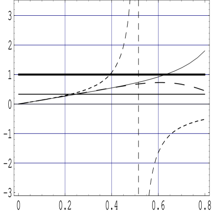
Figure 1: The entropy/energy ratios for our configuration, in the two different regimes of $\mu_{eff}$, namely $0<\mu_{eff}^{2}<1$ (long dash curve) and $-1<\mu_{eff}^{2}<0$ (short dash curve), as compared with the conformal case (thin full line) and with the Bekenstein and Verlinde bounds (thicker line and second thicker one, respectively).

The horizontal axis is $\delta$ and the vertical one is the ratio entropy/energy. The thicker line is the upper limit of Bekenstein’s ratio $S\left(\beta\right)/2\pi r\widetilde{E}\left(\beta\right)=1$. The thinner of the thick lines is the Verlinde ratio $S\left(\beta\right)/2\pi r\widetilde{E}\left(\beta\right)=1/3$. The thin full curve is the conformal result. The long-dashed curve plot is Eq. (76) and the short-dashed one Eq. (77); in both cases we have set $\mu_{eff}^{2}=\left|\mu_{eff}^{2}\right|=0.5$. For $\delta\rightarrow 0$ the plots corresponding to Eqs. (76), (77), and the conformal case all coalesce into the same straight line. Notice that for $\delta\approx 0.2$ all entropy bounds exceed the Verlinde bound. The one corresponding to the conformal limit surpases quite soon the Bekenstein bound, at about $\delta\approx 0.6$. Concerning our approach, it is very interesting to remark that, owing to the different algebraic signs of the effective mass corrections, the entropy bounds given by Eqs. (76) and (77) behave in a very different way. Indeed, with negative (tachyonic) effective mass, the entropy bound soon exceeds ($\delta\approx 0.4$) the Bekenstein bound (as in the case of the conformal theory). Here, this is probably the manifestation of some tachyonic-related instability, that renders also another branch of negative values of the ratio. Notice the sudden jump for $\delta\approx 0.5$. This behaviour also seems to be related to such tachyonic instabilituy and is due to the fact that the energy becomes negative. The entropy remains always positive, as remarked before. However, because we are on the verge of violating the validity of our approximation the behaviour for $\delta>0.5$ is suspicious and could be spurious. At the same time, for positive effective mass the entropy bound remains below the Bekenstein bound for all values of $\delta$, which is a remarkable result. What is more, the value seems to come back to fulfill Verlinde’s bound, for higher values of $\delta$, which is indeed very nice.

From Eq. (47) we can also obtain the entropy/energy ratio in the limit $m_{eff}\beta\gg 1$. In fact, it is easy to show that in this limit the entropy/energy ratio does not depend on the effective mass $m_{eff}$ and reads

$$\frac{S\left(\beta\right)}{2\pi r\widetilde{E}\left(\beta\right)}\approx\frac{5}{3}\delta\,.$$ (78)

Therefore, in the high-temperature regime ($\delta\rightarrow 0)$, with $m_{eff}\gg T$, the ratio entropy/energy remains bounded by the Bekenstein limit. It should be expected that a similar bound will hold for the de Sitter graviton in the early thermal universe.

5 Concluding remarks

In this work, we have considered the evaluation of of the Casimir energy at zero and finite temperature for the case of a massive scalar field in $\mathbf{S}^{1}\times\mathbf{S}^{3}$ geometries allowing for an arbitrary conformal parameter $\xi$.

The evaluation of the corresponding thermodynamical functions through the rescaled Abel-Plana sum formula leads straightforwardly to the very high temperature regime (no exponential corrections), but then, it is there that the relevant physics lies. As stressed in Ref. [10], it is only in the high-T regime that we are allowed to make use of thermodynamical methods in the one-loop approximation [19] (for earlier studies of similar questions see Ref. [20] where a slightly different approach was employed). We have also shown that for $\mu_{eff}^{2}=0$, the zero temperature Casimir energy is degenerated in the sense that it is equal to the Casimir energy of the conformal case. We also have evaluated the relevant thermodynamical functions and extended the previous analysis of entropy bounds and entropy-energy ratios of the symmetrical conformal case to the present one. Interestingly enough, for $\mu_{eff}^{2}=0$, all previous results concerning Bekenstein-Verlinde ratios are valid. Also, dual symmetries, as for example the temperature inversion symmetry, are recovered.

Our results can be used in the calculation of the entropy/energy ratio for the graviton living in the same spacetime. Since the cosmological constant will play the role of the effective mass considered here, it follows that the entropy/energy ratio will depend on the cosmological constant. Moreover, since a ‘cosmological constant’ term coming from the vacuum fluctuations of some field (as predicted by several fashionable models) will depend on time, as the radius of the universe also does, this bound will become time-dependent. We can speculate then on the relation between the change of such a kind of cosmological constant and the evolution of the entropy bound.

As a final remark, notice that the free energy calculated here can be used in the analysis of the back reaction of a massive scalar field in the spacetime under discussion.

Acknowledgments

The authors are indebted with Sergei Odintsov for important suggestions and very helpful comments. A. C. T. wishes to acknowledge the kind hospitality of the Institut d’Estudis Espacials de Catalunya (IEEC/CSIC) and the Universitat de Barcelona, Departament d’Estructura i Constituents de la Matèria. A. C. T. also acknowledges the financial support of Consejo Superior de Investigación Científica (CSIC, Spain), and of CAPES, the Brazilian agency for faculty improvement, Grant BExt 06832/01-2. The investigation of E.E. has been supported by DGI/SGPI (Spain), project BFM2000-0810, and by CIRIT (Generalitat de Catalunya), contracts 2002BEAI400019, 2001ACES00014 and 2001SGR-00427.

References

- [1] G. F. R. Ellis and R. Maartens, gr-qc/0211082.
- [2] J. D. Bekenstein, Phys. Rev. D 23 (1981) 287.
- [3] R. Brustein, S. Foffa, and G. Veneziano, hep-th/0101083, Phys. Lett. B 507 (2001) 270.
- [4] E. Verlinde, hep-th/00084140 v2.
- [5] B. Wang, E. Abdalla and R.-K. Su, hep-th/0101073, Phys. Lett. B 503 (2001) 394; S. Nojiri, O. Obregon, S. D. Odintsov, H. Quevedo and M. P. Ryan, hep-th/0105052, Mod. Phys. Lett. 16 (2001) 1181; D. Youm, hep-th/0201268, Phys. Lett. B531 (2002) 276; R.-G. Cai and Y. S. Myung, hep-th/0210272; U. Danielsson, hep-th/0110265, JHEP 0203 (2002) 020.
- [6] D. Kutasov and F. Larsen, hep-th/0009244, JHEP0101 (2001) 01.
- [7] D. Klemm, A. C. Petkou and G. Siopsis, Nucl. Phys. B 601 (2000) 380.
- [8] F.-L. Lin, hep-th/0010127, Phys. Rev. D 63 (2001) 064026.
- [9] S. Nojiri and S. D. Odintsov, hep-th/0011115, Int. J. Mod. Phys. A16 (2001) 3273; S. Nojiri and S. D. Odintsov, hep-th/0103078, Class. Q. Grav. 18 (2001) 5227.
- [10] I. Brevik, K. A. Milton and S. D. Odintsov, hep-th/0202048 v4. Ann. of Phys. 302 (2002) 120.
- [11] K. A. Milton, The Casimir Effect: Physical Manifestations of Zero-Point Energy (World Scientific, Singapore, 2001); M. Bordag, U. Mohideen, and V. M. Mostepanenko, Phys. Rep. 353 (2001) 1; E. Elizalde and A. Romeo, Am. J. Phys. 59 (1991) 711.
- [12] I.L. Buchbinder, S.D. Odintsov and I.L. Shapiro, Effective Action in Quantum Gravity (A. Hilger, Bristol, 1992).
- [13] E. Elizalde, S. D. Odintsov, A. Romeo, A. A. Bytsenko and S. Zerbini, Zeta function regularization techniques with applications (World Scientific, Singapore, 1994); E. Elizalde: Ten Physical Applications of Spectral Zeta Functions (Springer-Verlag, Berlin, 1995).
- [14] E. Elizalde and A. C. Tort, Phys. Rev. D 66 (2002) 045033.
- [15] A. Erdélyi, W. Magnus, F. Oberhettinger, and F. Tricomi, Higher Transcendental Functions (McGraw-Hill, New York, 1953).
- [16] I. S. Gradshteyn and I. M. Ryzhik, Table of Integrals, Series, and Products, 5th ed. (Academic Press, San Diego, 1994).
- [17] M. Abramowitz and I. Stegun, Handbook of Mathematical Functions with Formulas, Graphs and Mathematical Tables, 9th printing, (Dover, New York)
- [18] K. Kirsten and E. Elizalde, Phys. Lett. B 365 (1996) 72.
- [19] S. Das, P. Majundar and R. K. Bhaduri, Class. Quant. Grav. 19 (2002) 2355.
- [20] J. S. Dowker, Phys. Rev. D 37 (1988) 558.