Integrable quantum field theories with supergroup symmetries: the $OSP(1/2)$ case.

Abstract

As a step to understand general patterns of integrability in $1+1$ quantum field theories with supergroup symmetry, we study in details the case of $OSP(1/2)$. Our results include the solutions of natural generalizations of models with ordinary group symmetry: the $UOSP(1/2)_{k}$ WZW model with a current current perturbation, the $UOSP(1/2)$ principal chiral model, and the $UOSP(1/2)\otimes UOSP(1/2)/UOSP(1/2)$ coset models perturbed by the adjoint. Graded parafermions are also discussed. A pattern peculiar to supergroups is the emergence of another class of models, whose simplest representative is the $OSP(1/2)/OSP(0/2)$ sigma model, where the (non unitary) orthosymplectic symmetry is realized non linearly (and can be spontaneously broken). For most models, we provide an integrable lattice realization. We show in particular that integrable $osp(1/2)$ spin chains with integer spin flow to $UOSP(1/2)$ WZW models in the continuum limit, hence providing what is to our knowledge the first physical realization of a super WZW model.

1 Introduction

Two dimensional quantum field theories with supergroup symmetries have played an increasingly important role in our attempts to understand phase transitions in 2D disordered systems - some recent works in this direction are [1, 2, 3, 4, 5, 6, 7, 8].

These theories however prove quite difficult to tackle. Attempts at non perturbative approaches using conformal invariance [3, 8] or exact S matrices [9, 10, 11] have been popular recently, but so far, very few complete results are available. This paper is the second of a series (started with [9]) on models with orthosymplectic symmetry. Our goal is to relate and identify the different pieces of the theoretical puzzle available - sigma models, Wess Zumino Witten (WZW) models and Gross Neveu (GN) models, integrable lattice models, and exactly factorized S matrices - and to find out which physical systems they describe, and which peculiarities arise from the existence of supergroup symmetries. In our first paper [9], we studied among other things the $OSP(1/2)$ Gross Neveu model and the $OSP(1/2)/OSP(0/2)$ supersphere sigma model. A physical realization for the latter was identified in [12] in terms of a lattice loop model with self intersections, based on an earlier work of [13]. Other such realizations for different models or supergroups have yet to be made. In the case of ordinary algebras, integrable lattice models do provide such realizations, and are closely related with WZW and GN models based on the corresponding groups [14]. This relation is also important, for technical reasons, in the solution of the Principal Chiral Models (PCM) [15].

The main result of this paper is an analysis of integrable lattice models based on the $osp(1/2)$ superalgebra, and the associated field theories. While the general pattern is not unlike the case of ordinary groups, important differences are also encountered.

In section 2, we show that the continuum limit of the model based on the fundamental representation is not the GN (or WZW model) but the supersphere sigma model, generalizing the observation of [12].

In section 3 and 4 we show that that, for integer spin, the continuum limit is the $UOSP(1/2)$ WZW model at integer level - in particular, the spin $1$ quantum spin chain flows to the $UOSP$ level one model. This provides, to our knowledge, the first physical realization of a super WZW model. We also find that for odd spin $s$, the continuum limit, like for $s=1$, is not a WZW model. Attempts are made in section 6 to identify the corresponding field theories, based on the expectation that in these cases, the orthosymplectic symmetry is realized non linearly.

The $UOSP(1/2)$ PCM model is discussed in section 5, and the $UOSP(1/2)/U(1)$ models and associated parafermions in section 7.

2 Integrable lattice models with $osp(1/2)$ symmetry

Our conventions for the $osp(1/2)$ algebra [16] are summarized in the appendix . We start with the integrable model based on the fundamental representation $\rho_{1/2}$. The highest weight vector is denoted by $|1/2,1/2>$, and we shall treat it as fermionic, so the super dimension of this representation is equal to $-1$ . The product of two spin $1/2$ representations decomposes into a spin 0, a spin 1/2 and a spin 1 representation. Their highest weights are respectively bosonic, fermionic, and bosonic. The graded permutation operator reads

$$P=-P_{1}+P_{1/2}+P_{0}$$ (1)

and the Casimir

$$2C=3P_{1}+P_{1/2}\equiv 3-2P_{1/2}-3P_{0}$$ (2)

The hamiltonian of the integrable model is defined on the space $\rho_{1/2}^{\otimes N}$ as [17, 18, 19]

$$H=-c\sum_{i}{4\over 3}(P_{0})_{i,i+1}+2(P_{1/2})_{i,i+1}$$ (3)

(where $(P_{j})_{i,i+1}$ denotes the projector onto spin $j$ in the tensor product of the representations at site $i,i+1$, $c$ is a normalization constant related with the sound velocity) is integrable, and corresponds to the anisotropic limit of the integrable $osp(1/2)$ vertex model one can deduce from the scattering matrix of [9]. The Bethe ansatz equations for this model read schematically

$$\left({\lambda-i/2\over\lambda+i/2}\right)^{N}=\epsilon\prod{\lambda-\lambda^{\prime}-i\over\lambda-\lambda^{\prime}+i}\prod{\lambda-\lambda^{\prime}+i/2\over\lambda-\lambda^{\prime}-i/2}$$ (4)

(where the $\lambda$’s are the roots) and the energy

$$E=-c\sum{1\over\lambda^{2}+1/4}$$ (5)

The sign $\epsilon$ depends on the boundary conditions for the hamiltonian, and has not, in our opinion, always been correctly interpreted in the literature [18]. The point is that a hamiltonian with $osp(1/2)$ symmetry will be obtained by having the last term in the sum involve the projectors $(P_{j})_{N,N+1}$, and identifying the states in the $N+1^{th}$ space with the ones in the first space. In the case of superalgebras, this is not exactly the same as having the projectors $(P_{j})_{N,1}$: the difference involves ‘passing generators’ through the $N$ first states in the tensor product, and this can of course generate signs. The hamiltonian with $osp(1/2)$ symmetry corresponds to the Bethe equations with $\epsilon=1$ in (4). This agrees with the original results in [17]. Antiperiodic boundary conditions for the fermions would correspond to $\epsilon=-1$ instead.

According to Martins [18], when $\epsilon=1$, the ground state of the $S^{z}=0$ coincides with the one of the $S^{z}=1/2$ sector , leading to a degeneracy of 4 for the state $h=\bar{h}=0$. The central charge read in that sector is $c=-2$. The total partition function (that is, the trace of $q^{(H+P)/2}\bar{q}^{(H-P)/2}$, $P$ the momentum, and for $\epsilon=1$ again) reads from [18]

$$Z = 4\left|q^{1/12}\prod_{n=1}^{\infty}(1+q^{n})^{2}\right|^{2}$$ (6)

$$= {1\over\eta\bar{\eta}}\sum_{m\in 2Z,e\in Z+1/2}q^{(2e+m)^{2}/8}\bar{q}^{(2e-m)^{2}/8}$$

This is in agreement with the interpretation of the low energy limit of this lattice model with a symplectic fermion theory, as was proposed in [12]. In the latter paper, this identification was made by using the fact that the hamiltonian is the anisotropic limit of a vertex model which can be reinterpreted as a loop model, and thus as a model of classical $OSP(1/2)$ spins in two dimensions, similar to the one used in the analysis of the usual $O(n)$ model. It was then argued that the integrable hamiltonian lies in the broken symmetry Goldstone phase, and that the low energy limit is the weak coupling limit of the supersphere sigma model, whose target space is $S^{(0,2)}=OSP(1/2)/[OSP(0/2)\equiv SP(2)]$ (the equivalent of $O(N)/O(N-1)$ for $N=-1$). Recall one can easily parametrize this target space using $x=1-\eta_{1}\eta_{2}$ such that $x^{2}+2\eta_{1}\eta_{2}=1$. The sigma model action (Boltzmann weight $e^{-S}$) is

$$S={1\over g}\int d^{2}x\left[(\partial_{\mu}x)^{2}+2\partial_{\mu}\eta_{1}\partial_{\mu}\eta_{2}\right]$$ (7)

with the beta function $\beta\propto-3g^{2}$. At small coupling, the action reduces to the symplectic fermions theory, and the partition function (6) coincides with the determinant of the Laplacian with periodic boundary conditions in the space direction and antiperiodic boundary conditions in the “time” direction (along which the trace is taken). For $g$ negative, the model flows to weak coupling in the UV, and is massive in the IR, where symmetry is restored. The action reads then, in terms of the fermion variables, and after trivial rescalings,

$$S=-{1\over|g|}\int d^{2}x\left[\partial_{\mu}\eta_{1}\partial_{\mu}\eta_{2}-\eta_{1}\eta_{2}\partial_{\mu}\eta_{1}\partial_{\mu}\eta_{2}\right]$$ (8)

Notice that the relative normalization of the two terms can be changed at will by changing the normalization of the fermions. The relative sign can also be changed by switching the fermion labels $1\rightarrow 2$. However, the sign of the four fermion term cannot be changed, and determines whether the model is massive or massless in the IR. For $g$ positive, the model flows (perturbatively) to weak coupling in the IR. This is the case of the lattice model introduced in [13, 18].

It is possible to generalize the integrable model by introducing heterogeneities in a way well understood for ordinary algebras [20]. In doing so, the source term in the equations (4) is replaced by

$$\left({\lambda-\Lambda-i/2\over\lambda-\Lambda+i/2}\right)^{N/2}\left({\lambda+\Lambda-i/2\over\lambda+\Lambda+i/2}\right)^{N/2}$$ (9)

where $\Lambda$ is a parameter measuring heterogeneities, and the energy becomes

$$E=-{c\over 2}\sum{1\over(\lambda-\Lambda)^{2}+1/4}+{1\over(\lambda+\Lambda)^{2}+1/4}$$ (10)

We will not discuss complete calculations here, but simply derive some essential features of the associated thermodynamics Bethe ansatz (TBA). The ground state is made of real particles, and excitations are holes in the ground state. After introducing the Frourier transforms

$$\hat{f}(x)=\int d\lambda e^{i\lambda x}f(\lambda),~{}~{}f(\lambda)={1\over 2\pi}\int dxe^{-i\lambda x}\hat{f}(x)$$ (11)

the physical equations read

$$\hat{\rho}+\hat{\rho}^{h}={\cos\Lambda x\over 2\cosh(x/2)-1}-e^{-|x|/4}{\sinh(x/2)\over\cosh(3x/4)}\hat{\rho}^{h}$$ (12)

and the energy, up to a constant

$$E={c\over 2\pi}\int\hat{\rho}(x){\cos\Lambda x\over 2\cosh(x/2)-1}dx$$ (13)

The interesting way to proceed then is to take the limit $N\rightarrow\infty$, $a\rightarrow 0$ ($a$ the lattice spacing), such that $Na\rightarrow L$ finite. We then take the limit $\Lambda\rightarrow\infty$ with $e^{-2\Lambda\pi/3}/a$ finite. In that limit, excitations at finite rapidity acquire a relativistic dispersion relation, with rapidity $\theta={2\pi\over 3}\lambda$. The scattering of these excitations with themselves corresponds to the $S$ matrix element:

$$S\equiv\Sigma_{0}=-\exp\left[i\int_{-\infty}^{\infty}{d\omega\over\omega}e^{-3i\omega/\pi}e^{-|\omega|/2}{\sinh\omega\over\cosh(3\omega/2)}\right]$$ (14)

and the latter coincides with $\sigma_{3}^{+}-\sigma_{2}^{+}$, the scattering matrix element of particle 1 with itself in the sigma model (7), as discussed in [9] (this matrix element is called $\Sigma_{0}$ there).

In fact, one can check that the thermodynamics of the spin chain, in this limit, coincides with the thermodynamics of the field theory for the supersphere sigma model discussed in [9]: the introduction of heterogeneities provides thus a regularization of this field theory.

As always - and this can be related [21] to the Nielsen-Ninomiya theorem [22] - the massive degrees of freedom near vanishing bare rapidity in the model with heterogenities are completed by massless degrees of freedom at large bare rapidities (edges of the Brillouin zone). These are the same massless modes that would be present in the homogeneous chain obtained by letting $\Lambda=0$. The dynamics of these massless modes decouples entirely from the dynamics of the massive ones, and one can identify the associated CFT with the weak coupling limit of the supersphere sigma model, that is, the symplectic fermion theory.

It is tempting to carry out the same procedure for the case of higher spin. Unfortunately, not much is known about the higher spin integrable $osp$ spin chains in explicit form. It is fair to expect, based on analogies with other cases - in particular the $so(n)$ case - that such chains do exist, and are described by changing the source terms and energy terms as

$${\lambda-i/2\over\lambda+i/2}\rightarrow{\lambda-si\over\lambda+si},~{}~{}~{}{1\over\lambda^{2}+1/4}\rightarrow{2s\over\lambda^{2}+s^{2}}$$ (15)

where $s$ is the higher spin. The thermodynamics of the massive field theory limit is described by the equations

$${\epsilon_{j}(\theta)\over T}=\phi(\theta-\theta^{\prime})*\ln\left(1+e^{\epsilon_{j}(\theta^{\prime})/T}\right)-\sum_{l=1}^{\infty}\left(\delta_{j,l+1}+\delta_{j,l-1}\right)\phi(\theta-\theta^{\prime})*\ln\left(1+e^{-\epsilon_{l}(\theta^{\prime})/T}\right)$$ (16)

where $\phi(\theta)={3\over 2\cosh 3\theta/2}$ and $f*g(\theta)={1\over 2\pi}\int f(\theta-\theta^{\prime})g(\theta^{\prime})d\theta^{\prime}$. The boundary condition $\epsilon_{2s}\rightarrow m\cosh\theta$ must be imposed. The free energy reads then

$$F=-T\int{d\theta\over 2\pi}m\cosh\theta\ln\left(1+e^{-\epsilon_{2s}/T}\right)$$ (17)

The thermodynamics of the lattice model is described by similar equations, but different source terms. It allows one in particular to determine the entropy per site of the chain in the large $T$ limit. One finds that this entropy corresponds, for $s$ half integer, to a mix of representations $\rho_{1/2},\rho_{3/2},\ldots,\rho_{s}$, and for $s$ integer, a mix of representations $\rho_{0},\rho_{1},\ldots,\rho_{s}$. The integrable models must therefore involve these mix of representations on every site, and presumably must be considered as having $osp$ super-Yangian symmetry, in analogy with the $so(n)$ case [23]. In particular, the extension of the adjoint by a scalar representation to form an irreducible representation of the Yangian is typical. Calculations with a twist angle giving antiperiodic boundary conditions to the kinks shows that the representations with half-integer spin have superdimension $-1$, while those with integer spin have superdimension $+1$. Some of these results have been obtained independently and using a different approach in [19].

It is easy to check that the central charge of these models is

$$c_{eff}={8s\over 2s+3}$$ (18)

As in the usual $su(2)$ case, one can deform the models by considering $R$ matrices with $U_{q}osp(1/2)$ symmetry, and one can truncate them in the case $q$ a root of unity. The resulting TBA’s have the form shown in Figure 1 (with a total number of nodes equal to $N$), and central charge

$$c_{eff}={8s\over 2s+3}-{24s\over(N+4)(N+4-2s)}$$ (19)

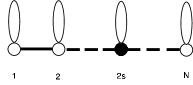
Figure 1: Incidence diagram of the general TBA obtained after quantum group deformation and truncation of the spin $s$ chain.

Most of the following is devoted to understanding the field theories associated with (18) and (19).

3 Coset models

The basic field theory we have introduced so far is the $OSP(1/2)/SP(2)$ non linear sigma model (7). Another type of sigma model plays a major role in the analysis: the $UOSP(1/2)_{k}$ Wess Zumino Witten model. Details about $OSP$ and $UOSP$ are furnished in the appendix: the bosonic part of $UOSP(1/2)$ is $SU(2)$, and the group is compact. The level $k$ is quantized (for the normalization of $k$, we use the level of the sub $SU(2)$, like for instance in the works [24]. The same model would be called the $OSP(1/2)_{-2k}$ model following the conventions used in the literature on disordered systems (see eg [25], as well as in our previous paper). The model is not expected to be a unitary conformal field theory: this is clear at the level of the action, where for instance the purely fermionic part is closely related to the $\eta\xi$ system, a non unitary theory. This is also expected on general grounds, since, for instance, there is no way to define a metric without negative norm (square) states in some representations.

It turns out however that the $UOSP(1/2)_{k}$ WZW theories are relatively simple, at least at first sight. The best way to understand them is to use a remarkable embedding discovered by Fan and Yu [26].

3.1 The $UOSP(1/2)/SU(2)$ coset models

These authors made the crucial observation that

$$UOSP(1,2)_{k}\approx SU(2)_{k}\times{UOSP(1,2)_{k}\over SU(2)_{k}}$$ (20)

where the branching functions of the latter part define a Virasoro minimal model, with

$$c_{uosp} = {2k\over 2k+3}$$

$$c_{su2} = {3k\over k+2}$$

$$c_{virasoro} = 1-6{(k+1)^{2}\over(k+2)(2k+3)}$$ (21)

Only for $k$ an integer does the action of the Wess Zumino model make sense, and we will restrict ourselves to this case in the following. The Virasoro models which appear there have $p=2k+3,q=k+2$; they are non unitary, and their effective central charge is $c_{eff}=1-{12\over(2k+3)(2k+4)}$. These models can thus be considered as $UOSP/SU$ coset models!

The perturbation of these models by the operator $\phi_{21}$ (here, the labels refer to the description as a Virasoro minimal model) with dimension $h=1-{3\over 4(k+2)}$ is well known to be integrable (the $1$ comes from the $OSP$, the $3/4(k+2)$ from the $SU(2)$). The TBA has the form shown in Figure 2 [27]. As observed in [9], it can be obtained after a q-deformation and a truncation of the basic supersphere sigma model TBA. The corresponding S matrices can thus easily be deduced, and follow RSOS restrictions of the q-deformed $a_{2}^{(2)}$ S matrices, or, equivalently, q-deformed $osp(1/2)^{(1)}$ S matrices. The simplest and most interesting case corresponds to the model of Virasoro minimal series $p=5,q=3$. Its central charge is $c=-3/5$ while $c_{eff}=3/5$. The TBA for a perturbation by the operator $\phi_{21}$ of weight $h=3/4$ is described by the diagram in the figure in the particular case where the number of nodes is two. The S matrix has been worked out in details in [28].

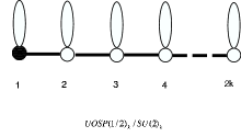
Figure 2: Incidence diagram of the TBA describing $UOSP(1/2)_{k}/SU(2)_{k}$ coset models perturbed by the operator with $h=1-{3\over 4(k+2)}$. The total number of nodes is $2k$.

An amusing consequence of this observation is that the supersphere sigma model appears as the limit $k\rightarrow\infty$ of a series of coset models. This is quite similar to the way the ordinary sphere sigma model appears as the limit of a series of parafermion theories [29], this time of type $SU(2)_{k}/U(1)$.

An important difference between the two cases is that, since the three point function of $\phi_{21}$ vanishes, the perturbation of the coset models is independant of the sign of the coupling, and thus always massive. The situation was different in the case of parafermionic theories $SU(2)/U(1)$, where one sign was massive (and corresponded, in the limit $k\rightarrow\infty$, to the case $\theta=0$), but the other was massless [29] (and corresponded in the limit $k\rightarrow\infty$, to the case $\theta=\pi$). For the supersphere, there is no theta term, so it is natural that we get only one flow.

An interesting consequence of the embedding is that we can deduce the effective central charge of the $UOSP(1/2)$ WZW model at level $k$. Using that for the Virasoro model, $c_{eff}=1-{12\over(2k+2)(2k+3)}$, one finds

$$c_{eff}={8k\over 2k+3},~{}~{}~{}UOSP(1/2)_{k}$$ (22)

This result will be compatible with all the subsequent analysis, but it is in slight disagreement with [24, 26]. In the latter papers, conjectures are made that the spectrum closes on primary fields of spin $j=0,{1\over 2},\ldots,{k\over 2}$ with dimension $h={j(2j+1)\over 2k+3}$. If this turned out to be true, the models we identify would not exactly be the WZW models, but maybe some “extensions” of these - at the present time, this issue is not settled, but it seems simpler to assume the value (22) is indeed the effective central charge of the WZW model.

3.2 The $UOSP(1/2)\times SU(2)/SU(2)$ coset models

We consider now TBA’s with a total number of nodes $N=2k+2l$. If the massive node is the $2k^{th}$ one, the UV central charge is

$$c_{eff} = {8k\over 2k+3}-{24k\over(2k+2l+4)(2l+4)}$$ (23)

$$= {8k\over 2k+3}+{3l\over l+2}-{3(l+k)\over l+k+2}$$

suggesting that the model can be understood as a coset model $UOSP(1/2)_{k}\otimes SU(2)_{l}/SU(2)_{k+l}$. Assuming the TBA corresponds to a theory perturbed by an operator whose odd point functions vanish, we find the dimension of the perturbing operator to be $h=1-{3\over 4(k+l+2)}$. This is compatible with taking the spin $1/2$ field in the denominator of the coset.

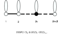
Figure 3: Incidence diagram of the TBA describing $UOSP(1/2)_{k}\otimes SU(2)_{l}/SU(2)_{k+l}$ coset models perturbed by the operator with $h=1-{3\over 4(k+l+2)}$. The total number of nodes is $2k+2l$.

If the massive node is the $2k+1^{th}$ one meanwhile, the central charge is

$$c_{eff} = {8k+4\over 2k+4}-{12(2k+1)\over(2k+2l+4)(2l+3)}$$ (24)

$$= {3k\over k+2}+{8l\over 2l+3}-{3(k+l)\over k+l+2}$$

suggesting similarly that the model can be understood as a coset $SU(2)_{k}\otimes UOSP(1/2)_{l}/SU(2)_{k+l}$ perturbed by the operator of dimension $h=1-{3\over 4(k+l+2)}$. Of course the two cases are actually equivalent by taking mirror images, but it is convenient to keep them separate to study the large $l$ limit later.

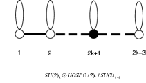
Figure 4: Incidence diagram of the TBA describing $SU(2)_{k}\otimes UOSP(1/2)_{l}/SU(2)_{k+l}$ coset models perturbed by the operator with $h=1-{3\over 4(k+l+2)}$. The total number of nodes is $2k+2l$.

3.3 The $UOSP(1/2)\otimes UOSP(1/2)/UOSP(1/2)$ models.

We now consider instead TBA’s with a total number of nodes $N=2k+2l-1$. If the massive node is the $2k^{th}$ one, the UV central charge is found to be

$$c_{eff} = {8k\over 2k+3}-{24k\over(2l+3)(2k+2l+3)}$$ (25)

$$= {8k\over 2k+3}+{8l\over 2l+3}-{8(k+l)\over 2k+2l+3}$$

suggesting that the models can be interpreted as coset $UOSP(1/2)_{k}\otimes UOSP(1/2)_{l}/UOSP(1/2)_{k+l}$. Assuming the TBA corresponds to a theory perturbed by an operator whose odd point functions do not vanish, we find the dimension of the perturbing operator to be $h=1-{3\over 2k+2l+3)}$. This is compatible with taking the spin $1/2$ field in the denominator of the coset.

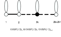
Figure 5: Incidence diagram of the TBA describing $UOSP(1/2)_{k}\otimes UOSP(1/2)_{l}/UOSP(1/2)_{k+l}$ coset models perturbed by the operator with $h=1-{3\over 2k+2l+3}$. The total number of nodes is $2k+2l-1$.

Note that, since we have assumed the three point function of the perturbing operator does not vanish, switching the sign of the perturbation should lead to a different result. It is natural to expect that one has then a massless flow, whose TBA and S matrices are readily built by analogy with the $SU(2)$ case [30]: we leave this to the reader as an exercise.

Finally, we notice that the $UOSP(1/2)$ coset model with $k=l=1$ was first identified in the paper [31].

3.4 The other models

The last possible case we can obtain out of this construction corresponds to a TBA’s with an odd number of nodes (say, $2k+1$), and the mass on an odd node, too.

The effective central charge is $c_{eff}=1-{12\over(2k+5)(2k+4)}$. The models can be considered as Virasoro models with $p=2k+5,q=k+2$, and the TBA corresponds to perturbation by the $\phi_{15}$ field now, of dimension $h_{15}=1-{3\over 2k+5}$. We have not found any convincing way to interpret this in terms of $OSP(1/2)$ cosets; maybe it is not possible. Notice that the $3/(2k+5)$ is a weight for $OSP_{k+1}$, which, since it appears with a minus sign in $h$, should be in the denominator of the sought after coset. Notice also that, by using the remark at the end of the previous paragraph, we expect flows between the models we have interpreted in terms of $OSP(1/2)$ and $SU(2)$ cosets and these unidentified models. This could be a useful hint.

4 Sigma models

4.1 The $UOSP$ WZW models

Taking $l\rightarrow\infty$ for the class of models where the massive node is an even one, we obtain theories with central charge $c_{eff}={8k\over 2k+3}$. This value coincides with the result obtained in the first section for $s=k$. We therefore suggest that the continuum limit of the lattice models with integer spin $s$ are the $UOSP(1/2)_{k=s}$ models. Introducing heterogeneities then gives rise to the current-current perturbation of these models.

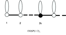
Figure 6: Incidence diagram of the TBA describing the $UOSP(1/2)_{k}$ WZW model with a current current perturbation.

The S matrix is the tensor product of the RSOS S matrix for the Virasoro model $M_{2k+3,k+2}$ perturbed by $\phi_{21}$ (which we saw can be reinterpreted as an $UOSP$ RSOS matrix) and the supersphere sigma model S matrix.

These results apply to the NS sector of the model, where the fermionic currents have integer modes, and are periodic. The Ramond sector can be obtained by spectral flow; one has in particular [26]

$$L_{0}^{R}=L_{0}^{NS}-J_{3}^{0,NS}+{k\over 4}$$ (26)

While the true central charge seems inaccessible from the TBA, one can follow the spectral flow by giving a fugacity to the solitons, as was discussed in our first paper, ie calculating $Z=\hbox{Tr}\left[e^{-\beta H}e^{i\alpha q/(t-1)}\right]$, where $q$ is the topological charge of the solitons, normalized as $q=0,\pm 1$. Antiperiodic boundary conditions correspond to $\alpha=(t-1)\pi$, and are found to give, using the system of equations (38,39) of our previous paper

$$c_{{eff}}={8k\over 2k+3}-6k$$ (27)

in agreement with (26).

Finally, it is easy to check from the TBA that the dimension of the perturbing operator has to be $(1,1)$. This gives strong support to our conjecture.

We stress that, as far as we know, none of the perturbed $UOSP(1/2)_{k}$ WZW models can be interpreted as a Gross-Neveu model. The $OSP$ GN models correspond to models with, formally, level $k=-{1\over 2}$, and have a different physics, and different scattering matrices, as discussed in [9]. We will get back to this issue in the conclusion.

4.2 The “$SU(2)_{k}\otimes UOSP(1/2)/SU(2)$” models.

If we take the limit $l\rightarrow\infty$ for models which have the mass on an odd node, the central charge as well as the interpretation of the coset models are consistent with a theory of the form $SU(2)_{k}\otimes UOSP(1/2)/SU(2)$, of which the supersphere sigma model was just the simplest ($k=0$) version.

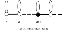
Figure 7: Incidence diagram of the TBA describing the $SU(2)_{k}\otimes UOSP(1/2)/SU(2)$ sigma model.

It would be most interesting to find out the action describing these models, but we have not done so for now - we will comment about the problem below.

5 The $UOSP(1/2)$ PCM model

In the $SU(2)$ case for instance, the limit $k\rightarrow\infty$ of the WZW model with a current current perturbation coincides with the scattering theory for the PCM (principal chiral model) model [15]. It is natural to expect that the same thing will hold for the $UOSP(1/2)$ case. The TBA looks as in Figure 8, and the scattering matrix has obviously the form $S_{PCM}\propto S\otimes S$, where $S$ is the S matrix for the supersphere sigma model, up to CDD factors we will discuss below

Figure 8: Incidence diagram of the TBA describing the $OSP(1/2)$ PCM model.

Let us study this PCM model more explicitely. It is convenient to write an element of $UOSP(1/2)$ as

$$g=\left(\begin{array}[]{ccc}1+{1\over 4}\eta\eta^{\diamond}&-{1\over 2}\eta&{1\over 2}\eta^{\diamond}\\ -{1\over 2}(a\eta^{\diamond}-b^{\diamond}\eta)&a(1-{1\over 8}\eta\eta^{\diamond})&-b^{\diamond}(1-{1\over 8}\eta\eta^{\diamond})\\ -{1\over 2}(b\eta^{\diamond}+a^{\diamond}\eta)&b(1-{1\over 8}\eta\eta^{\diamond})&a^{\diamond}(1-{1\over 8}\eta\eta^{\diamond})\end{array}\right)$$ (28)

with the constraint $aa^{\diamond}+bb^{\diamond}=1$. In a similar way, the conjugate of the matrix, $g^{\ddagger}$, reads

$$g^{\ddagger}=\left(\begin{array}[]{ccc}1+{1\over 4}\eta\eta^{\diamond}&{1\over 2}(b\eta^{\diamond}+a^{\diamond}\eta)&-{1\over 2}(a\eta^{\diamond}-b^{\diamond}\eta\\ {1\over 2}\eta^{\diamond}&a^{\diamond}(1-{1\over 8}\eta\eta^{\diamond})&b^{\diamond}(1-{1\over 8}\eta\eta^{\diamond})\\ {1\over 2}\eta&-b(1-{1\over 8}\eta\eta^{\diamond})&a(1-{1\over 8}\eta\eta^{\diamond})\end{array}\right)$$ (29)

The action of the PCM model reads, after a rescaling of the fermions $\eta\rightarrow 2\eta$

$$-Str\left(\partial_{\mu}g\partial_{\mu}g^{\dagger}\right)\propto\partial_{\mu}\eta\partial_{\mu}\eta^{\diamond}+\left(\partial_{\mu}a\partial_{\mu}a^{\diamond}+\partial_{\mu}b\partial_{\mu}b^{\diamond}\right)\left(1-\eta\eta^{\diamond}\right)+{1\over 2}\eta\eta^{\diamond}\partial_{\mu}\eta\partial_{\mu}\eta^{\diamond}$$ (30)

We note that the $UOSP(1/2)$ group manifold can be identified with the supersphere $S^{3,2}$[32], that is, the space $OSP(4/2)/OSP(3/2)$. The PCM model, however, cannot be expected to coincide with the sigma model on $S^{3,2}$: the symmetry groups are different, and so are the invariant actions. For instance, in the PCM model, the group $UOSP(1/2)$ acts by conjugation, leaving the identity invariant. In the vicinity of the identity, under the $SP(2)=SU(2)$, the fermionic coordinates transform as a doublet, and the bosonic coordinates transform as a triplet. In the sigma model, the coordinates near the origin transform as the fundamental of $OSP(3/2)$. Under the $SO(3)=SP(2)=SU(2)$ of the $OSP(3/2)$, the bosonic coordinates transform as a triplet but the fermionic coordinates now transform as a singlet (they form a doublet under a different $SP(2)$, which leaves the sphere $S^{3}$ invariant). The groups acting differently, the invariant actions can be expected to be different. This is confirmed by explicit calculation. The supersphere $S^{3,2}$ can be parametrized in terms of coordinates $x_{i}$, $i=0,\ldots,3$ and $\eta_{1},\eta_{2}$. The constraint $\sum_{0}^{3}x_{i}^{2}+2\eta_{1}\eta_{2}=1$ gives rise to

$$x_{i}=y_{i}\left(1-\eta_{1}\eta_{2}\right),~{}~{}\sum_{0}^{3}y_{i}^{2}=1$$ (31)

The sigma model action

$$S=2\partial_{\mu}\eta_{1}\partial_{\mu}\eta_{2}+\sum_{i=0}^{3}(\partial_{\mu}x_{i})^{2}$$ (32)

becomes then

$$S=2\partial_{\mu}\eta_{1}\partial_{\mu}\eta_{2}+\left(\sum_{i=0}^{3}\left(\partial_{\mu}y_{i}\right)^{2}\right)(1-2\eta_{1}\eta_{2})-2\eta_{1}\eta_{2}\partial_{\mu}\eta_{1}\partial_{\mu}\eta_{2}$$ (33)

The two equations (30,32) are similar, but exhibit a major difference in the sign of the four fermion term.

The physics of the two models is considerably different. For the supersphere sigma model, the $\beta$ function is exactly zero to all orders, and the theory is exactly conformal invariant for any value of the coupling constant (like in the $O(2)/O(1)$ case). For the PCM, the $\beta$ function follows from Wegner’s calculations in the case $O(-1)$ [33]

$$\beta=3\lambda^{2}-{9\over 2}\lambda^{3}+{81\over 8}\lambda^{4}\ldots$$ (34)

to be compared eg with the $SU(2)$ case

$$\beta=-2\lambda^{2}-2\lambda^{3}-3\lambda^{4}+\ldots$$ (35)

The conventions here are that the Boltzmann weight is $\exp\left(-S\right)$, and

$$S=-{1\over 2\lambda}\int Tr~{}(Str~{})\left[\partial_{\mu}g\partial_{\mu}g^{\dagger}\right]={1\over 2\lambda}\int Tr\left[g^{-1}\partial_{\mu}g\right]^{2}$$

In the $SU(2)$ case, the massive theory corresponds to $\lambda<0$. By contrast, for the $OSP(1/2)$ case, the massive direction corresponds to $\lambda>0$. However, since one takes then a supertrace instead of a trace, the $SU(2)$ part of the PCM action has the same sign as in the $SU(2)$ pure case, with Boltzmann weight $\exp[-|cst|\int(\partial_{\mu}a\partial_{\mu}a^{\dagger}+\partial_{\mu}b\partial_{\mu}b^{\dagger})]$, and the functional integral is well defined. Note that the symplectic fermion part of the Boltzmann weight is of the form $\exp[-|cst|\int(\partial_{\mu}\eta\partial_{\mu}\eta^{\diamond}+\eta\eta^{\diamond}\partial_{\mu}\eta\partial_{\mu}\eta^{\diamond})]$, and also exhibits the same sign as the action of the supersphere sigma model in the massive phase (where the symmetry is restored).

The exact S matrix can be deduced from the TBA by noticing that, for the matrix $S\otimes S$, the presence of the self coupling for the first node in the sigma model TBA would lead to a double self coupling. This has to be removed, and the usual calculation gives

$$S_{PCM}=Y~{}S_{\sigma}\otimes S_{\sigma}$$ (36)

where the CDD factor $\hat{Y}={\sinh\omega+\sinh 2\omega\over\sinh 3\omega}$, $Y={\sinh\theta+i\sin(\pi/3)\over\sinh\theta-i\sin(\pi/3}$ cancels the double poles and double zeroes in $\Sigma_{0}^{2}$ (14). Let us recall for completeness the sigma model S matrix.

$$\check{S}_{i_{1}j_{1}}^{j_{2}i_{2}}=\sigma_{1}E+\sigma_{2}P+\sigma_{3}I$$ (37)

where we have set

$$E_{i_{1}j_{1}}^{j_{2}i_{2}}=\delta_{i_{1},\bar{j}_{1}}\delta^{i_{2},\bar{j}_{2}}(-1)^{x(i_{1})}(-1)^{x(i_{2})}$$ (38)

while $P$ is the graded permutation operator

$$P_{i_{1}j_{1}}^{j_{2}i_{2}}=(-1)^{p(i_{1})p(j_{1})}\delta_{i_{1}}^{i_{2}}\delta_{j_{1}}^{j_{2}}$$ (39)

The indices $i$ take values in the fundamental representation of the $osp(1/2)$ algebra, $i=1,2,3$. We set $\bar{1}=1,\bar{2}=3,\bar{3}=2$, $x(1)=x(3)=0,x(2)=1$. The factors $\sigma$ in (37) read

$$\sigma_{1} = -{2i\pi\over(N-2)(i\pi-\theta)}~{}\sigma_{2}$$

$$\sigma_{3} = -{2i\pi\over(N-2)\theta}~{}\sigma_{2}$$ (40)

for the value $N=1-2=-1$ characteristic of the $OSP(1/2)$ case.

6 Realizations of the $UOSP(1/2)$ symmetry.

In section 4, we have found two families of models whose $S$ matrix has $UOSP(1/2)$ symmetry . The models based on the lattice TBA for $s$ integer correspond to $UOSP(1/2)_{k=s}$ WZW models peturbed by a current current interaction. The UV theory is a current algebra, in which the symmetry is locally realized by two sets of currents, $J^{\pm,0},j^{\pm}$ and $\bar{J}^{\pm,0},\bar{j}^{\pm}$.

What happens in the other family of models is less clear. An exception to this is the case $s=1/2$, ie the $UOSP(1/2)/SU(2)\equiv OSP(1/2)/SP(2)$ sigma model. In this case, the symemtry is realized non linearly, and it is worthwhile seeing more explicitely how this works.

6.1 Symplectic fermions and non linearly realized symmetries

Consider thus the supersphere sigma model. This model for positive coupling describes the Goldstone phase for $OSP(1/2)$ symmetry broken down spontaneously to $SP(2)$ (possible since the group is not unitary compact). For negative coupling, it is massive, and the $OSP(1/2)$ symmetry is restored at large distance. In either case, the action is proportional to (we have slightly changed the normalizations compared with the previous paper)

$$S\propto 2\partial_{\mu}\eta_{1}\partial_{\mu}\eta_{2}+(\partial_{\mu}x)^{2}$$ (41)

with $2\eta_{1}\eta_{2}+x^{2}=1$. We can find the Noether currents with the usual procedure. An infinitesimal $OSP(1/2)$ transformation reads

$$\delta x = -\delta\xi_{1}\eta_{1}+\delta\xi_{2}\eta_{2}$$

$$\delta\eta_{1} = -\delta\xi_{2}x+\delta a\eta_{1}+\delta c\eta_{2}$$

$$\delta\eta_{2} = -\delta\xi_{1}x+\delta b\eta_{1}-\delta a\eta_{2}$$ (42)

where $\delta\xi_{1},\delta\xi_{2}$ are ‘small’ fermionic deformation parameters, $\delta a,\delta c$ small bosonic parameters. By definition, this change leaves $2\eta_{1}\eta_{2}+x^{2}$ invariant. In terms of the fermion variables, the symmetry is realized non linearly:

$$\delta\eta_{1}=-\delta\xi_{2}(1-\eta_{1}\eta_{2})+\delta a\eta_{1}+\delta c\eta_{2}$$

$$\delta\eta_{2}=-\delta\xi_{1}(1-\eta_{1}\eta_{2})+\delta a\eta_{1}-\delta a\eta_{2}$$ (43)

Performing the change in the action, and identifying the coefficients of linear derivatives $\partial_{\mu}\eta_{i},\partial_{\mu}x$ with the currents gives five conserved currents. Three of them generate the sub $su(2)$:

$$J^{+} = -{1\over 2}\eta_{1}\partial\eta_{1}$$

$$J^{-} = {1\over 2}\eta_{2}\partial\eta_{2}$$

$$J^{3} = {1\over 4}\left(\eta_{1}\partial\eta_{2}-\partial\eta_{1}\eta_{2}\right)$$ (44)

The two fermionic currents meanwhile are

$$j^{+}=\partial_{\mu}x~{}\eta_{1}-x~{}\partial_{\mu}\eta_{1}=\partial_{\mu}\eta_{1}(1-2\eta_{1}\eta_{2})$$

$$j^{-}=\partial_{\mu}x~{}\eta_{2}-x~{}\partial_{\mu}\eta_{2}=\partial_{\mu}\eta_{2}(1-2\eta_{1}\eta_{2})$$ (45)

These five currents should be present in the UV limit of the sigma model, which coincides with symplectic fermions. The latter theory has been studied a great deal. Of particular interest is the operator content, which is conveniently encoded in the generating function (6). Recall that the “ground state” (that is, fields of weight $(0,0)$) is degenerate four times, while there are eight fields of weight $(1,0)$ (and eight fields of weight $(0,1)$). It has sixteen fields of weight $(1,1)$. We can understand these multiplicities easily by using the sigma model interpretation. From the $OSP(1/2)$ symmetry, we expect to have, by taking the weak coupling limit of the foregoing currents, five fields $(1,0)$ and five fields $(0,1)$ (these fields are not chiral currents, because of some logarithmic festures: more about this below). Meanwhile, the broken $OSP(1/2)$ symmetry implies the existence of three non trivial fields with weight $(0,0)$, whose derivatives are also necessarily ‘currents’. We therefore expect eight fields ($8=$ fundamental $+$ adjoint) $(1,0)$ and $(0,1)$, in agreement with the known result.

Note that fields with weights $(1,0)$ and $(0,1)$ can have some common components due to the presence of fields with vanishing weights. It follows that many of their products do actually vanish, leading to a multiplicity of sixteen for fields $(1,1)$, and not $8^{2}$, as one could have naively assumed.

An interesting question is now what remains of the $OSP(1/2)$ symmetry right at the weak coupling fixed point, that is, in the symplectic fermions theory itself. There, it turns out that only the sub $SP(2)$ can be observed, as the bosonic currents $J^{\pm},J^{3}$ are still conserved in the symplectic fermion theory. This conservation boils down to the equations of motion $\partial_{\mu}\partial^{\mu}\eta_{i}=0$. If one naively tries to check the conservation of the fermionic currents, it seems one needs $\partial_{\mu}\partial^{\mu}(\eta_{1}\eta_{2})=0$, which is manifestly wrong! So these currents, which are conserved in the sigma model at any non zero coupling, are not strictly speaking conserved right at the weak coupling fixed point.

The explanation of this apparent paradox lies in the role of the coupling constant and how exactly one can obtain the conformal limit. The best is to take the Boltzmann weight as $e^{-S}$ with $S$ as above, $S=2\partial_{\mu}\eta_{1}\partial_{\mu}\eta_{2}+(\partial_{\mu}x)^{2}$ and put the coupling constant in the radius of the supersphere $x^{2}+2\eta_{1}\eta_{2}=g^{2}$, which now leads to $x=g-{1\over g}\eta_{1}\eta_{2}$. The equations of motion are

$$\partial_{\mu}\partial^{\mu}~{}x = \lambda x$$

$$\partial_{\mu}\partial^{\mu}~{}\eta_{1} = \lambda\eta_{1}$$

$$\partial_{\mu}\partial^{\mu}~{}\eta_{2} = \lambda\eta_{2}$$ (46)

where

$$\lambda={1\over g^{2}}\left[x\partial_{\mu}\partial^{\mu}~{}x+\eta_{1}\partial_{\mu}\partial^{\mu}\eta_{2}+\partial_{\mu}\partial^{\mu}\eta_{1}\eta_{2}\right]$$ (47)

leading, as usual, to the conservation of $j^{\pm}$. The conformal symplectic fermion theory is then obtained in the (singular) limit $g\rightarrow\infty$, where the field $x$ formally becomes a constant, and $\partial_{\mu}\partial^{\mu}x=0$ a triviality. Within this limit, the $OSP(1/2)$ symmetry is lost, but one gets as its remnant the two fermionic “currents”, $\partial_{\mu}\eta_{1}$ and $\partial_{\mu}\eta_{2}$.

It is interesting finally to discuss the algebra satisfied by the $SP(2)$ currents right at the conformal point (a related calculation has been presented in [34], but we do not think its interpretation - based on rescaling the currents- is appropriate). The OPE’s are rather complicated:

$$J^{+}(z)J^{-}(w) = {1\over 4}{1+2\ln|z-w|+\eta_{2}\eta_{1}\over(z-w)^{2}}-{1\over 8}{\partial(\eta_{1}\eta_{2})+{\bar{z}-\bar{w}\over z-w}\bar{\partial}(\eta_{1}\eta_{2})\over z-w}-{1\over 2}\ln|z-w|\partial\eta_{1}\partial\eta_{2}$$ (48)

$$+ {{3\over 2}J^{3}+{1\over 2}{z-w\over\bar{z}-\bar{z}}\bar{J}^{3}\over z-w}$$

$$J^{3}(z)J^{\pm}(w) = \pm{{3\over 4}J^{\pm}+{1\over 4}{\bar{z}-\bar{w}\over z-w}\bar{J}^{\pm}\over z-w}$$

$$J^{3}(z)J^{3}(w) = {1\over 8}{1+2\ln|z-w|+\eta_{2}\eta_{1}\over(z-w)^{2}}-{1\over 16}{\partial(\eta_{1}\eta_{2})+{\bar{z}-\bar{w}\over z-w}\bar{\partial}(\eta_{1}\eta_{2})\over z-w}-{1\over 4}\ln|z-w|\partial\eta_{1}\partial\eta_{2}$$

and we see that the notation $J(z)$ is abusive: the field has weights $(1,0)$ but the OPEs involve $\ln\bar{z}$ terms. The commutators of charges are only affected by the ${1\over z-w}$ term, and the $su(2)$ relations are recovered not through a rescaling but because of the presence of other non trivial OPEs between the ‘left’ and ‘right’ components. For instance, writing only the relevant term, one has

$$J^{+}(z)\bar{J}^{-}(w) = {1\over 2(z-w)}\bar{J}^{3}+{1\over 2(\bar{z}-\bar{w})}J^{3}$$

$$\bar{J}^{+}(z)\bar{J}^{-}(w) = {1\over 2(z-w)}\bar{J}^{3}+{1\over 2(\bar{z}-\bar{w})}J$$

$$\bar{J}^{+}(z)\bar{J}^{-}(w) = {{3\over 2}\bar{J}^{3}\over\bar{z}-\bar{w}}$$ (49)

ensuring $[Q^{+},Q^{-}]=2Q^{3}$, where $Q={1\over 2i\pi}\int(Jdz-\bar{J}d\bar{z})$.

Amusingly, the $1/(z-w)^{2}$ part of the OPEs corresponds to the normalization $k={1\over 2}$, so the UV limit of the sigma model does contain a “logarithmic $k=1/2$” $su(2)$ current algebra.

6.2 Speculations on the $SU(2)_{k}\otimes UOSP(1/2)/SU(2)$.

It is tempting to speculate then that the models for $s$ half integer correspond to “higher level” generalizations of the symplectic fermions, with a non linear realization of the $UOSP(1/2)$ symmetry, and a “logarithmic $su(2)$ current algebra”. We do not know what the action of these models might be, except that in the UV they should reduce to the tensor product of a $SU(2)_{k}$ WZW model and symplectic fermions. Notice of course that the PCM model - the limit $k\rightarrow\infty$, does obey this scenario. Indeed, the PCM model also provides a realization of the $UOSP(1/2)$ symmetry which is non linear once the constraints have been explicitely solved. Solving the constraints in terms of the fermions gives

$$J^{+} = {1\over 2}\left[b\partial a^{\diamond}-a^{\diamond}\partial b-{b^{2}\over 4}\eta^{\diamond}\partial\eta^{\diamond}{(a^{\diamond})^{2}\over 4}\eta\partial\eta-{ba^{\diamond}\over 4}\left(\eta\partial\eta^{\diamond}+\eta^{\diamond}\partial\eta\right)\right]$$

$$J^{-} = {1\over 2}\left[a\partial b^{\diamond}-b^{\diamond}\partial a+{a^{2}\over 4}\eta^{\diamond}\partial\eta^{\diamond}+{(b^{\diamond})^{2}\over 4}\eta\partial\eta-{ab^{\diamond}\over 4}\left(\eta\partial\eta^{\diamond}+\eta^{\diamond}\partial\eta\right)\right]$$

$$J^{3} = 2\left[a\partial a^{\diamond}+b^{\diamond}\partial b+{1\over 4}\left(ab\eta^{\diamond}\partial\eta^{\diamond}-a^{\diamond}b^{\diamond}\eta\partial\eta\right)+{aa^{\diamond}\over 8}\left(\partial\eta\eta^{\diamond}-\eta\partial\eta^{\diamond}\right)\right.$$

$$\left.~{}~{}~{}+{bb^{\diamond}\over 8}\left(\eta\partial\eta^{\diamond}-\partial\eta\eta^{\diamond}\right)\right]$$ (50)

The fermionic currents meanwhile read

$$j^{+} = -{1\over 2}\left(b\partial\eta^{\diamond}+a^{\diamond}\partial\eta\right)-{b\over 16}\eta\eta^{\diamond}\partial\eta^{\diamond}-{a^{\diamond}\over 16}\eta\eta^{\diamond}\partial\eta$$

$$j^{-} = -{1\over 2}\left(b^{\diamond}\partial\eta-a\partial\eta^{\diamond}\right)+{1\over 16}a\eta\eta^{\diamond}\partial\eta^{\diamond}-{b^{\diamond}\over 16}\eta\eta^{\diamond}\partial\eta$$ (51)

One can as well solve for the bosonic constraint $aa^{\diamond}+bb^{\diamond}=1$. If one does so, and rescales the fields with the coupling constant as in the supersphere case, the UV expression of the currents becomes simply the sum of the currents for a system of 3 bosons (the small coupling limit of the $SU(2)$ PCM model) and the currents for the symplectic fermion theory.

The evidence from the TBA is that the PCM model can give rise to two kinds of models (more on this in the conclusion): either the $UOSP(1/2)_{k}$ WZW models like in the usual case, but also the $SU(2)_{k}\otimes UOSP(1/2)/SU(2)$ model, which presumably involves some sort of term changing the $SU(2)$ part of the action into the WZW one with a current current perturbation, but leaving the symplectic fermionic part essentially unaffected. We do not know how to concretely realize this though.

Another interesting aspect stems from the fact that the central charge obtained by giving antiperiodic boundary conditions to the kinks reads, after elementary algebra,

$$c=1-6{(k+1)^{2}\over(k+2)}$$ (52)

This is precisely the central charge of the models $M_{k+2,1}$, of which the first two have $c=-1$ and $c=-7$. We are thus led to speculate that the $M_{k+2,1}$ models - or rather, their proper ‘non minimal’ versions (studied in [35], although we do not necessarily agree with the conclusions there), as the minimal models are entirely empty in this case, are models with spontaneously broken $UOSP(1/2)$ symmetry. It would be very interesting to look further for signs of an $UOSP$ structure in these models, and to study their ‘logarithmic’ $SU(2)$ algebra.

Note that these models are obtained by hamiltonian reduction of the $SU(2)_{k}$ model. In this reduction [36], an auxiliary $\eta\xi$ system is introduced to play the role of Fadeev-Popov ghosts, so these models are indeed naturally related to the product of $SU(2)_{k}$ and $U(1)$ as we observed earlier.

7 The $UOSP(1/2)/U(1)$ sigma model(s)

Instead of factoring out the $SU(2)$, one can of course also factor out the $U(1)$ and get an $UOSP(1/2)/U(1)$ sigma model. This is especially interesting since the standard argument to derive the continuum limit of the $osp(1/2)$ spin chains would lead to a sigma model on the manifold parametrizing the coherent states, and this is precisely $UOSP(1/2)/U(1)$ [37, 38].

Note however that the manifold $UOSP(1/2)/U(1)$ is not a symmetric (super) space (this can easily be seen since the (anti) commutator of two fermionic generators does not always belong to the Lie algebra of $U(1)$). As a consequence, sigma models on this manifold will have more than one coupling constant.

To proceed, a possible strategy is to follow [29] and consider for a while models $UOSP(1/2)_{k}/U(1)$, that is graded parafermionic theories.

Graded parafermions [39] theories are constructed in a way similar to the original construction of Fateev and Zamolodchikov, with the additional ingredient of a $Z_{2}$ grading. They obey the OPE rules

$$\psi_{l}(z)\psi_{l^{\prime}}(w)=(-1)^{p(l)p(l^{\prime})}\exp\left(2i\pi{ll^{\prime}\over k}\right)\psi_{l^{\prime}}(w)\psi_{l}(z)$$ (53)

Their dimensions are $h_{l}={l(k-l)\over k}+{\epsilon(l)\over 2}$, where $\epsilon=1$, $l$ half an odd integer, $\epsilon=0$ otherwise. Of particular interest is the OPE

$$\psi_{1/2}(z)\psi_{-1/2}(w) = (z-w)^{{1\over 2k}-2}\left[1+(z-w)^{2}O^{(1/2)}+\ldots\right]$$

$$\psi_{1}(z)\psi_{-1}(w) = (z-w)^{{2\over k}-2}\left[1+(z-w)^{2}O^{(1)}+\ldots\right]$$

Here, the operators $O$ have dimension 2, and must obey $O^{(1)}-O^{(2)}={2k+3\over 2k}T$, $T$ the stress energy tensor. The simplest parafermionic theory for $k=1$ has $c=-{3\over 5}$, and seems to coincide with the model $M_{5,3}$ . For $k$ an integer, $l$ runs over the set $l=-k+{1\over 2},\ldots,0,\ldots,k-{1\over 2}$, $2l\in Z$. Parafermions with integer $l$ are bosonic, the others are fermionic. For $k=1$, $\psi_{1}\equiv I$, and there is only a pair of parafermionic fields, of weight $h={3\over 4}$. It can be shown that the parafermionic theories just defined coincide with $UOSP(1/2)_{k}/U(1)$ coset theories.

Like in the $SU(2)_{k}$ case, the $UOSP(1/2)_{k}$ model with a current-current pertubation can be written in terms of the graded parafermions and a free boson $\phi$. It is then easy to find an integrable anisotropic deformation

$$\psi_{1}\bar{\psi}_{1}e^{i\beta\sqrt{2\over k}\phi}+\psi_{-1/2}\bar{\psi}_{-1/2}e^{-{i\over\sqrt{2k}}\beta\phi}$$ (55)

(In the case $k=1$, the perturbation reads $e^{-i\sqrt{2}\beta\phi}+\psi_{1/2}\bar{\psi}_{1/2}e^{{i\over\sqrt{2}}\beta\phi}$. ) The non local conserved currents [40] are $\psi_{-1}e^{-i\sqrt{2\over k}{\varphi\over\beta}}$ and $\psi_{1/2}e^{{i\over\sqrt{2k}}{\varphi\over\beta}}$ (where $\varphi$ denotes the right component of $\phi=\varphi+\bar{\varphi}$). The TBA and S matrices are rather obvious: we take the same left part of the diagram as for the $OSP(1/2)_{k}$ case, but replace the infinite right tail by the ubiquitous, finite and anisotropic part discussed in our first paper. In the isotropic limit [40] $\beta^{2}\rightarrow 1$, the RG generates the other terms necessary to make (55) into a whole current current perturbation.

Taking the limit $\beta\rightarrow 0$ would then lead to the TBA for the parafermionic theory. This would require an understanding of the scattering in the attractive regime where bound states exist, but we have not performed the related analysis. It is possible however to make a simple conjecture based on numerology, and analogies with the $SU(2)$ case. Consider indeed the TBA in Figure 9

Figure 9: Conjectured incidence diagram of the TBA describing the $UOSP(1/2)_{k}/U(1)$ parafermions.

where the box represents the set of couplings discussed in our first paper [9]. In the UV, the diagram is identical to the one arising in the study of the $a_{2}^{(2)}$ Toda theory. The central charge is $c_{1}=2k-1$ as discussed in [9]. In the IR, the diagram is identical to the ones arising in the $UOSP/SU$ coset models, and $c_{2}=2k-4+{12\over 2k+3}$. The final central charge is thus $c_{eff}=3-{12\over 2k+3}$, and concides with the effective central charge for $UOSP(1/2)/U(1)$ parafermions of level $k$. We conjecture this TBA describes the perturbation of these parafermionic theories by the combination of graded parafermions

$$\psi_{1}\bar{\psi}_{1}+\psi_{-1/2}\bar{\psi}_{-1/2}$$ (56)

The effective dimension of the perturbation deduced from the TBA is $1-{1\over 2k}$, and this coincides with the combination $h={2h_{1}+h_{2}\over 3}$. Note that we have not studied what kind of scattering theory would give rise to the TBA in Figure 9, and whether it is actually meaningful. Still, taking the limit $k\rightarrow\infty$, we should obtain the TBA for something that looks like an $UOSP(1/2)/U(1)$ sigma model. Notice that the bosonic part of this model is identical with the $SU(2)/U(1)$ sigma model, and thus there is the possibility of a topological term. It is not clear what the low energy limit of the model with topological angle $\theta=\pi$ would be.

8 Conclusions

The results presented here presumably have rather simple generalization to the $OSP(1/2n)$ case, even though details might not be absolutely straightforward to work out - for instance, we do not know of embeddings generalizing the one discussed in the first sections.

The supersphere sigma model for $g$ positive in the conventions of section 2, flows in the IR to weak coupling, at least perturbatively. It is expected that the phase diagram will exhibit a critical point at some value $g^{*}$ and that for larger coupling, the theory will be massive. The critical point presumably coincides with the dilute $O(N=-1)$ theory first solved by Nienhuis [41]. This theory is described by a free boson with a charge at infinity, and is closely related with the minimal model $M_{5,3}$. In fact the partition function of the dilute $O(N=-1)$ model provided one restricts to even numbers of non contractible loops can be written in the Coulomb gas language of Di Francesco et al. [42] as

$$Z_{5,3}={1\over 2}\left[Z_{c}(3/5,5)-Z_{c}(3/5,1)\right]$$ (57)

and coincides with the partition function of the minimal model. Earlier in this paper, we have identified this model with the $UOSP(1/2)_{1}/U(1)$ parafermionic theory. The full $O(N=-1)$ theory, however defined, has a considerably more complex operator content [43].

Note that antiperiodic boundary conditions for the fermions, which give an effective central charge equal to $c_{eff}=1$ in the supersphere sigma model give, in the critical theory, a highly irrational value $c_{eff}=1-{18\over\pi^{2}}\left(\hbox{arccosh}(3/2)\right)^{2}$. There are no indications that an integrable flow from the critical theory to the low temperature generic theory exists. An integrable flow is known to exist in the special case where the symmetry is enhanced to $SU(1/2)$. In that case, the IR theory is the so called dense $O(N=-1)$ model, which has $c=-7$, and is closely related with the minimal model $M_{3,1}$. Note that this model is the second model of the unidentified series in section 4, and bears some formal resemblance to the model $UOSP(1/2)_{3/2}$. What this means remains one of the many open questions in this still baffling area.

Acknowledgments: We thank G. Landi, N. Read and M. Zirnbauer for useful remarks and suggestions. We especially thank P. Dorey for pointing out the discussion of $OSP$ coset models in [31]. The work of HS was supported in part by the DOE.

Appendix A Some results on $osp(1/2)$.

We collect in this appendix some formulas about $osp(1/2)$, the associated current algebra and groups.

The supergroup $OSP(1/2)$ is the group of ‘real’ matrices $g$ obeying (basic references are [44, 45, 46])

$$g^{st}~{}J~{}g=J$$ (58)

where

$$J=\left(\begin{array}[]{ccc}1&0&0\\ 0&0&1\\ 0&-1&0\end{array}\right)$$ (59)

Elements of the group preserve the quadratic form, if $X=(b,\theta_{1},\theta_{2})$, $X.X^{\prime}=bb^{\prime}+\theta_{1}\theta_{2}^{\prime}-\theta_{2}\theta_{1}^{\prime}$. They can be parametrized by $g=e^{A}$ with

$$A=\left(\begin{array}[]{ccc}0&-\eta_{1}&-\eta_{2}\\ \eta_{2}&a&c\\ -\eta_{1}&b&-a\end{array}\right)$$ (60)

Here no complex conjugation is ever needed: $a,b,c$ are real numbers, and $\eta_{1},\eta_{2}$ are ‘real’ Grassman numbers.

The group $UOSP(1/2)$ in contrast is made of complex supertransformations satisfying

$$g^{st}~{}J~{}g=J,~{}~{}g~{}g^{\ddagger}=1$$ (61)

To define the adjoint $M^{\ddagger}$, we first need to introduce a complex conjugation denoted by $\diamond$. It is, technically, a graded involution, which coincides with complex conjugation for pure complex numbers, $c^{\diamond}=\bar{c}$, $c\in C$, and obeys in general

$$(xy)^{\diamond}=x^{\diamond}y^{\diamond}$$

$$(x^{\diamond})^{\diamond}=(-)^{p(x)}x$$

$$(cx)^{\diamond}=\bar{c}x^{\diamond}$$ (62)

One then sets $g^{\ddagger}=\left(g^{st}\right)^{\diamond}$ , so $g$ in $UOSP(1/2)$ preserves in addition the form $X^{\diamond}X^{\prime}=\bar{b}b^{\prime}+\theta_{1}^{\diamond}\theta_{1}^{\prime}-\theta_{2}^{\diamond}\theta_{2}^{\prime}$.

One has now $g=e^{A}$ with

$$A=\left(\begin{array}[]{ccc}0&-\eta&-\eta^{\diamond}\\ \eta^{\diamond}&ia&ib\\ -\eta&ib^{\diamond}&-ia\end{array}\right)$$ (63)

with $a$ real, $a^{\diamond}=a$. The fermionic content of the supergroup is essentially unchanged, with $\eta\equiv\eta_{1}$, $\eta^{\diamond}\equiv\eta_{2}$. But the bosonic content is different: the non compact bosonic subgroup $SP(2)$ has been replaced by the compact one $SU(2)$.

The algebra $osp(1/2)$ is generated by operators which we denote $J^{3},J^{\pm}$ (bosonic) and $j^{\pm}$ (fermionic). Their commutation relations can be obtained from the current algebra given below by restricting to the zero modes. The casimir reads

$$C=(J^{3})^{2}+{1\over 2}\left(J^{+}J^{-}+J^{-}J^{+}\right)+{1\over 4}\left(j^{-}j^{+}-j^{+}j^{-}\right)$$ (64)

The representations of the super Lie algebra are labelled by an integer or half integer $j$, and are of dimension $4j+1$. The fundamental representation is three dimensional, and has spin $j=1/2$. It does contain a sub $sl(2)$ fundamental representation, following the pattern of $J^{3}=\hbox{diag}(0,-1/2,1/2)$. The generators $J^{\pm},J^{3}$ are bosonic. The fermionic generators are given by

$$j^{+}=\left(\begin{array}[]{ccc}0&-1&0\\ 0&0&0\\ -1&0&0\end{array}\right)~{}~{}~{}j^{-}=\left(\begin{array}[]{ccc}0&0&-1\\ 1&0&0\\ 0&0&0\end{array}\right)$$ (65)

The only metric compatible with $osp(1/2)$ requires the definition of a generalized adjoint satisfying (here $p=0,1$ denotes the parity) [45]

$$\left<A^{\dagger}\alpha|\beta\right>=(-1)^{p(A)p(\alpha)}\left<\alpha|A\beta\right>$$ (66)

and thus

$$(AB)^{\dagger}=(-1)^{p(A)p(B)}B^{\dagger}A^{\dagger}$$ (67)

It follows that $(J^{\pm})^{\dagger}=J^{\mp}$, $(J^{3})^{\dagger}=J^{3}$, while there remains some freedom for the fermionic generators, $(j^{+})^{\dagger}=\pm j^{-}$, $((j^{+})^{\dagger})^{\dagger}=-j^{+}$. It is in the nature of the algebra that negative norm square states will appear whatever the choice. Indeed, let us choose for instance

$$\left(j^{+}\right)^{\dagger}=j^{-},\left(j^{-}\right)^{\dagger}=-j^{+}$$ (68)

It then follows that the norm square of the state $|j,m>$ is

$$<j,m|j,m>=(-)^{2p(j)(j-m)}$$ (69)

Here, $p(j)=0$ if the highest weight state $|j,j>$ is bosonic, $p(j)=1$ if it is fermionic. Even if we start with the fundamental representation $j=1/2$ with $|1/2,1/2>$ bosonic, in the tensor product of this representation with itself, representations where the highest weight is fermionic will necessary appear. These do contain negative norm square states. In this paper, we will always choose the gradation for which $|1/2,1/2>$ is fermionic, and thus the fundamental representation has superdimension equal to $-1$.

The current algebra is defined by

$$\left[J^{3}_{n},J^{\pm}_{m}\right]=\pm J^{\pm}_{n+m} \left[J_{n}^{3},J_{m}^{0}\right]={k\over 2}n\delta_{n+m}$$

$$\left[J_{n}^{+},J_{m}^{-}\right] =kn\delta_{n+m}+2J^{3}_{n+m}$$

$$\left[J_{n}^{3},j_{m}^{\pm}\right]=\pm{1\over 2}j^{\pm}_{m+n} \left[J_{n}^{\pm},j_{m}^{\pm}\right]=0$$

$$\left[J_{n}^{\pm},j_{m}^{\mp}\right]=-j_{n+m}^{\pm} \left\{j_{n}^{\pm},j_{m}^{\pm}\right\}=\pm 2J_{n+m}^{\pm}$$

$$\left\{j_{n}^{+},j_{m}^{-}\right\} =2kn\delta_{n+m}+2J_{n+m}^{3}$$ (70)

Normalizations are such that the algebra contains a sub $sl(2)$ current algebra at level $k$.

The Wess Zumino Witten model on the supergroup $UOSP(1/2)$ corresponds to $k$ positive integer, and the sub $sl(2)$ current algebra to the WZW model $SU(2)_{k}$.

As commented in the text, the supersphere $S^{3,2}$ is the supermanifold of the supergroup $UOSP(1/2)$. It is also the total space of a principal fibration with structure group $U(1)$ and the quotient of this action is just the supersphere $S^{2,2}\approx UOSP(1/2)/U(1)$. The explicit realization is as follows [32]. Setting

$$x_{0} = (aa^{\diamond}-bb^{\diamond})\left(1-{1\over 4}\eta\eta^{\diamond}\right)$$

$$x_{1} = (ab^{\diamond}+ba^{\diamond}))\left(1-{1\over 4}\eta\eta^{\diamond}\right)$$

$$x_{2} = i(ab^{\diamond}-ba^{\diamond}))\left(1-{1\over 4}\eta\eta^{\diamond}\right)$$

$$\eta_{1} = -{1\over 2}(a\eta^{\diamond}+\eta b^{\diamond})$$

$$\eta_{2} = {1\over 2}(\eta a^{\diamond}-b\eta^{\diamond})$$ (71)

(these obey $x_{i}^{\diamond}=x_{i}$, and $\eta_{1}^{\diamond}=-\eta_{2}$) we obtain points in $S^{2,2}$, since $\sum(x_{i})^{2}+2\eta_{1}\eta_{2}=1$. Conversely, for a given point $x_{0},x_{1},x_{2},\eta_{1},\eta_{2}$ of $S^{2,2}$ one gets

$${1\over 2}\eta\eta^{\diamond} = \eta_{1}\eta_{2}$$

$$aa^{\diamond} = {1\over 2}\left[1+x_{0}(1+{1\over 2}\eta_{1}\eta_{2})\right]$$

$$bb^{\diamond} = {1\over 2}\left[1-x_{0}(1+{1\over 2}\eta_{1}\eta_{2})\right]$$

$$ab^{\diamond} = {1\over 2}(x_{1}-ix_{2})(1+{1\over 2}\eta_{1}\eta_{2})$$

$$\eta a^{\diamond} = -(x_{1}+ix_{2})\eta_{1}+(1+x_{0})\eta_{2}$$

$$\eta b^{\diamond} = (x_{1}-ix_{2})\eta_{2}-(1-x_{0})\eta_{1}$$ (72)

Define finally $U(1)=\{w,w\hbox{ bosonic },ww^{\diamond}=1\}$. Since the parametrization of (71) is invariant under $(a,b,\eta)\rightarrow(wa,wb,w\eta)$, this proves the statement.

Of course, the two spaces $UOSP(1/2)/U(1)$ and $S^{2,2}$ are not topologically equivalent: the fibration just discussed is in fact a ‘superextension’ of the Dirac monopole [32].

References

- [1] D. Bernard, “Conformal field theory applied to 2D disordered systems: an introduction”, hep-th/9509137.
- [2] C. Mudry, C. de C. Chamon and X. G. Wen, Nucl. Phys. B466 (1996) 383.
- [3] S. Guruswamy, A. Leclair and A. W. W. Ludwig, Nucl. Phys. B583 (2000) 475.
- [4] P. Fendley, “Critical points in two dimensional replica sigma models”, cond-mat/0006360
- [5] M. Zirnbauer, “Conformal field theory of the integer quantum Hall plateau transition”, hep-th/9905054.
- [6] A. Altland, B. D. Zimons and M. R. Zirnbauer, Phys. Rep. 359 (2002) 283; M. Bocquet, D. Serban and M. R. Zirnbauer, Nucl. Phys. B578 (2000) 628.
- [7] M. J. Bhaseen, J. S. Caux, I. I. Kogan and A. M. Tsvelik, Nucl. Phys. B618 (2001) 465.
- [8] D. Bernard and A. Leclair, Nucl. Phys. B628 (2002) 442.
- [9] H. Saleur and B. Wehefritz-Kaufmann, Nucl. Phys. B628 (2002) 407.
- [10] P. Fendley, “Taking to with S matrices”, cond-mat/0111582.
- [11] P. Fendley and N. Read, “Exact S matrices for supersymmetric sigma models and the Potts model”, hep-th/0207176.
- [12] J. L. Jacobsen, N. Read and H. Saleur, “Dense loops, supersymmetry and Goldstone phases in two dimensions”, cond-mat/0205033.
- [13] M. Martins, B. Nienhuis and R. Rietman, Phys. Rev. Lett. 81 (1988) 504.
- [14] I. Affleck, Nucl. Phys. B265 (1986) 409.
- [15] S. Polyakov and P. Wiegmann, Phys. Lett. B131 (1983) 121.
- [16] M. Scheunert, W. Nahm and V. Rittenberg, J. Math. Phys. 18 (1977) 146.
- [17] P. P. Kulish, J. Sov. Math. 35 (1986) 2648.
- [18] M. J. Martins, Nucl. Phys. B450 (1995) 768 ; Phys. Lett. B359 (1995) 334.
- [19] K. Sakai and S. Tsuboi, J. Phys. Soc. Jpn 70 (2001) 367; Int. J. Mod. Phys. A15 (2000).
- [20] C. Destri and H. de Vega, J. Phys. A22 (1989) 1329; N. Yu Reshetikhin and H. Saleur, Nucl. Phys. B419 (1994) 507.
- [21] C. Destri and T. Segalini, hep-th/9506120.
- [22] H. B. Nielsen, M. Ninomiya, Nucl. Phys. B185 (1981) 20.
- [23] N. Mac Kay, Nucl. Phys. B356 (1991) 729.
- [24] I.P.Ennes, A.V. Ramallo and J. M. Sanchez de Santos, “osp(1/2) Conformal Field Theory”, hep-th/9708094, in “Trends in theoretical physics (La Plata, 1997)”, Conf. Proc. 419, Amer. Inst. Phys., Woodbury, NY, (1998); Nucl. Phys. B491 (1997) 574; Nucl. Phys. B502 (1997) 671; Phys. Lett. B389 (1996) 485.
- [25] A. W.W. Ludwig, “A Free Field Representation of the Osp(2/2) current algebra at level k=-2, and Dirac Fermions in a random SU(2) gauge potential”, cond-mat/0012189.
- [26] J. Fan and M. Yu, “Modules Over Affine Lie Superalgebras”, hep-th/9304122.
- [27] F. Ravanini, M. Stanishkov and R. Tateo, Int. J. Mod. Phys. A11 (1996) 677.
- [28] G. Mussardo, Int. J. Mod. Phys. A7 (1992) 5027.
- [29] V. Fateev and Al. Zamolodchikov, Phys. Lett. B271 (1991) 91.
- [30] Al. Zamolodchikov, Nucl. Phys. B366 (1991) 122.
- [31] P. Dorey, A. Pocklington and R. Tateo, “INtegrable aspects of the scaling q-state Potts models I: bound states and bootstrap closure”, hep-th/0208111.
- [32] C. Bartocci, U. Bruzzo and G. Landi, J. Math. Phys. 31 (1990) 45; G. Landi, math-ph/9907020.
- [33] F. Wegner, Nucl. Phys. B316 (1989) 663.
- [34] I.I. Kogan and A. Nichols, “Stress energy tensor in logarithmic conformal field theories”, hep-th/0203207
- [35] M. Flohr, Int. J. Mod. Phys. A11 (1996) 4147.
- [36] M. Bershadsky and H. Ooguri, Comm. Math. Phys. 126 (1989) 49.
- [37] A. B. Balantekin, H. A. Schmitt and B. R. Barrett, J. Math. Phys. 29 (1988) 734.
- [38] A. Gradechi, J.Math.Phys. 34 (1993) 5951.
- [39] J.M. Camino, A.V. Ramallo and J.M. Sanchez de Santos, Nucl.Phys. B530 (1998) 715.
- [40] D. Bernard and A. Leclair, Comm. Math. Phys. 142 (1991) 359.
- [41] B. Nienhuis, Phys. Rev. Lett. 49 (1982) 1062.
- [42] P. di Francesco, H. Saleur and J.B. Zuber, J. Stat. Phys. 49 (1987) 57.
- [43] N. Read and H. Saleur, Nucl. Phys. B613 (2001) 409.
- [44] F.A. Berezin and V. N. Tolstoy, Comm. Math. Phys. 78 (1981) 409.
- [45] V. Rittenberg and M. Scheunert, J. Math. Phys. 19 (1978) 713.
- [46] L. Frappat, A. Sciarrino and P. Sorba, “Dictionary on Lie Superalgebras”, hep-th/9607161.