Abstract

We analyze the classical stability of string cosmologies driven by the dynamics of orientifold planes. These models are related to time–dependent orbifolds, and resolve the orbifold singularities which are otherwise problematic by introducing orientifold planes. In particular, we show that the instability discussed by Horowitz and Polchinski for pure orbifold models is resolved by the presence of the orientifolds. Moreover, we discuss the issue of stability of the cosmological Cauchy horizon, and we show that it is stable to small perturbations due to in–falling matter.

1 Introduction

Over the past year there has been a renewed interest in the study of time–dependent string backgrounds [1–33]. The main objective of this programme is to learn about the origin of the (possibly apparent) cosmological singularity using the powerful techniques of string theory. The logic behind this investigation was to start with an exact conformal field theory, e.g. strings in flat space, and to consider an orbifold of the theory with a time–dependent quotient space [34]. These simple orbifold constructions were, however, quite generally shown to be unstable by Horowitz and Polchinski [16] . These instabilities are associated to the formation of large black holes whenever a particle is coupled to the geometry and are non-perturbative in the string coupling. For this reason a perturbative string resolution of the time–dependent orbifold singularities seems inappropriate.

In [3] we investigated the orbifold of flat space–time by a boost and translation transformation. This orbifold suffers from the Horowitz–Polchinski instability. However, an aditional essential ingredient of the model was introduced in [9]: the time–like orbifold singularity is an orientifold, i.e. a brane with negative tension. One of the results that we shall show is that the orientifold provides precisely the non–perturbative string resolution of the singularity, modifying the gravitational interaction in its proximity. In fact, after briefly revising the Horowitz–Polchinski argument and the orientifold cosmology construction, we shall show in Section 4, with a tractable example in dimension $3$, that due to the presence of the orientifolds large black holes are not formed.

In any pre big–bang scenario, there is generically a possible classic instability associated with the propagation of matter through the bounce, which is analogous to the propagation of matter between the outer and inner horizons of charged black–holes [36, 37]. Let us consider a perturbation at some finite time in the far past, when the universe is contracting. In the case of orientifold cosmology there is a future cosmological horizon where the contracting phase ends (see also [38, 39, 40]), therefore one needs to worry about such perturbations diverging at the horizon, thus creating a big crunch space–time. We shall show in Section 5 that such perturbations remain finite (of course, they can grow and create small black holes, but this does not change the causal cosmological structure of the geometry). Furthermore, we shall see that the fluctuations that destabilize the geometry are precisely those that already destabilize the Minkowski vacuum.

2 The Horowitz–Polchinski Problem

In [16], Horowitz and Polchinski argue that a large class of time dependent orbifolds are unstable to small perturbations, due to large backreactions of the geometry. Their results, which overlap with the string theory scattering computations of [7, 14], do not rely on string theory arguments, and are obtained simply within the framework of classical general relativity.

The argument of Horowitz and Polchinski is quite simple and runs as follows. They analyze the orbifold of $D$–dimensional Minkowski space $\mathbb{M}^{D}$ by the action of a discrete isometry $e^{\kappa}$ where $\kappa$ is a Killing vector, and consider, in the quotient orbifold space $\mathbb{M}^{D}/e^{\kappa}$, a small perturbation. This perturbation naturally corresponds to an infinite sequence of perturbations in the covering space $\mathbb{M}^{D}$, related to each other by the action of $e^{\kappa}$. They consider, quite generally, a light ray with world–line $\Omega\subset\mathbb{M}^{3}$, together with all of its images

$$\Omega_{n}=\,e^{n\kappa}\Omega\,\ \ \ \ \ \ \ \ \ \ \ \ \ \ \ \ \ \ \ \ \ \ \ \ \ \left(n\in\mathbb{Z}\right)$$

for any integer $n$. The basic claim of [16] is that, for a wide range of time dependent orbifolds, the backreaction of gravity to the presence of this infinite sequence of light rays $\Omega_{n}$ will inevitably produce large black holes. As we already mentioned, this statement is a claim in pure classical gravity theory and to prove it Horowitz and Polchinski consider the scattering of two light rays $\Omega_{0}$ and $\Omega_{n}$. They compute, given $\kappa$, the impact parameter $b_{n}$ and the center of mass energy $\mathcal{E}_{n}$ of the scattering, and show that, for generic time dependent orbifolds, one has that $G\mathcal{E}_{n}\gg b_{n}^{D-3}$ for $n$ sufficiently large. The two image particles will be well within the Schwarzchild radius corresponding to the center of mass energy, and will form a black hole.

It is quite clear that, if the above argument is correct, it must hold also for a continuous distribution of light rays

$$e^{t\kappa}\Omega\,\ \ \ \ \ \ \ \ \ \ \ \ \ \ \ \ \ \ \ \ \ \ \ \ \ \left(t\in\mathbb{R}\right)$$ (1)

since the problematic interactions occur between rays separated by $\Delta t\gg 1$, and therefore should be completely insensitive to the distribution of the essentially parallel light rays when the parameter $t$ varies by $\Delta t\sim 1$. For continuous values of $t$, equation (1) defines a surface $S$ in $\mathbb{M}^{D}$, which we call the Horowitz–Polchinski (HP) surface. Again, the backreaction of gravity to the matter distribution on $S$ should form black holes by the previous argument. On the other hand, the continuous distribution is easier to treat analytically since it is invariant under the action of $\kappa$. Therefore, the full solution with the gravitational backreaction will also have $\kappa$ as a Killing vector. This fact simplifies explicit computations and therefore, from now on, we will only consider the continuous case.

In the rest of the paper we will be interested exclusively in a specific choice of orbifold, which describes, when correctly interpreted in $M$–theory, the dynamics of an orientifold/anti–orientifold pair. We postpone the discussion of the correct $M$–theory embedding and the crucial distinction between the orbifold and the orientifold interpretation to section 3, and we describe now the orbifold along the lines of [16].

We write $\mathbb{M}^{D}=\mathbb{M}^{3}\times\mathbb{E}^{D-3}$ and we parametrize $\mathbb{M}^{3}$ with coordinates $X^{\pm}$, $Y$, with line element

$$-dX^{+}dX^{-}+dY^{2}\,.$$ (2)

Points in $\mathbb{M}^{D}$ are identified along the orbits of the Killing vector field $\kappa$ which corresponds to boost in the $X^{\pm}$ plane and translation in the orthogonal direction $Y$

$$\kappa=X^{+}\partial_{+}-X^{-}\partial_{-}+\,\partial_{Y}\,.$$ (3)

For this special choice of $\kappa$ one has $b_{n}\sim n$ and $\mathcal{E}_{n}\sim e^{n}$ and the bound $G\mathcal{E}_{n}\gg b_{n}^{D-3}$ is always satisfied for $n$ large [16]. The directions along $\mathbb{E}^{D-3}$ then play no role (except to determine the strength of the gravitational interaction) and we will omit any reference to them, working effectively in three dimensions.

To study the geometry of the HP surface $S$, we parametrize the light ray $\Omega$ as

$$A^{a}+sV^{a}\text{\thinspace},$$

where $V^{a}$ is a null vector and $s$ is an affine parameter. If we consider the generic case when $V^{+}V^{-}\neq 0$ then, for some value of $t$, the image ray $e^{t\kappa}\Omega$ will be directed along the null vector $\left(1,1,1\right)$. This specific light ray on the surface $S$ will intersect the plane $X^{+}+X^{-}=0$ at a point with $X^{+}-X^{-}=2a$. By shifting the variables $s,t,Y$ so that this point corresponds to $s=t=Y=0$ we see that the surface $S$ is given by the following parametrization

$$X^{\pm} = \left(s\pm a\right)e^{\pm t}\,,$$ (4)

$$Y = \left(s+t\right)\,.$$

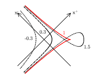
Figure 1: The curves given by equation (6), which represent the surfaces $S_{a}$ for the values of $a$ indicated in the figure. The surface $S_{1}$ is clearly singled out, and is the unique null surface.

The only free parameter which labels different surfaces is the constant $a$, and we will add a label $S_{a}$ to distinguish them. A convenient way to visualize $S_{a}$ is to move to coordinates

$$x^{\pm} = X^{\pm}e^{\mp Y}\,,$$ (5)

$$y = Y\,,$$

so that $\kappa=\frac{\partial}{\partial y}$. Then, since the surface $S_{a}$ is invariant under $\kappa$, it is given by a curve in the $x^{+},x^{-}$ plane (see Figure 1)

$$x^{\pm}=\left(s\pm a\right)e^{\mp s}.$$ (6)

This curve can also be viewed as the intersection of the surface $S_{a}$ with the plane $Y=0$ in $\mathbb{M}^{3}$.

Let us now describe some basic properties of the surfaces $S_{a}$. The induced metric is given by

$$2\left(1-a\right)dsdt+\left(s^{2}-a^{2}+1\right)dt^{2}$$

so it is timelike for all values of $a$ except for $a=1$, when $S$ is a null surface. For $a\neq 1$ the surfaces are smooth for any value of the parameters $s,t$. For $a=1$ the surface is, on the other hand, divided into two smooth parts for $s>0$ and $s<0$ which are joined along the singular line $s=0$. Moreover, the forward directed light cones, which are tangent to the null surface $S_{1}$, lie on one side of $S_{1}$ for $s>0$ and jump discontinuously, along the singular line $s=0$, to the other side of $S_{1}$ for $s<0$.

2.1 The Three–Dimensional Horowitz–Polchinski Problem

As we described in the previous section, we want to understand, in general, the gravitational backreaction to a distribution of light–rays in $\mathbb{M}^{3}\times\mathbb{E}^{D-3}$ distributed on the surface $S_{a}$ parametrized in $\mathbb{M}^{3}$ by (4) and fixed at a point along the spectator directions $\mathbb{E}^{D-3}$. For $D\geq 4$ gravity is non–trivial even in the absence of matter, and the problem is not soluble exactly. In $D=3$, on the other hand, space is curved only in the presence of matter and the problem is tractable.

Recall that the basic question is whether black holes are formed as a consequence of the strong gravitational interactions among the light rays. On the other hand, black holes in three dimensional flat space do not exist in the first place, and therefore it seems that the question is not well posed for $D=3$. This is not correct. In fact, the sign of the formation of a black hole in three dimensions is not the presence of a singularity but the existence, in the geometry, of closed timelike curves. To see this, recall again that, in a two–particle scattering with center of mass energy $\mathcal{E}$ and impact parameter $b$, a black hole forms when $G\mathcal{E}\gtrsim b^{D-3}$. For $D=3$ the threshold is then $G\mathcal{E}\gtrsim 1$ and is independent of the impact parameter $b$. To understand the meaning of this threshold, recall that the geometry describing the propagation of a single light ray in 3D is flat everywhere except along a null line, where curvature is concentrated. The local geometry is completely characterized by the holonomy in $SO\left(1,2\right)$ around the light ray, which is given by a specific null boost $U_{1}$. In the presence of a second light ray, we have a second holonomy null boost matrix $U_{2}$, as shown in Figure 2. The combined holonomy $U=U_{1}U_{2}$, on the other hand, depends on the center of mass energy of the two particles. For small center of mass energies $U$ is a rotation. On the other hand, when the center of mass energy exceeds the threshold value [43, 44, 45, 46], $U$ becomes a boost and closed timelike curves are formed which circle both particles, as shown in Figure 2. Finally, as shown in [41], one may consider the same dynamics in $AdS_{3}$ space, where black holes exist [47]. One then finds that, at exactly the same threshold, the scattering process creates, in the future, a BTZ black hole.

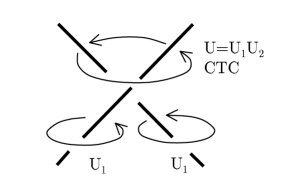
Figure 2: Scattering of light rays in three dimensions. The holonomies $U_{1}$ and $U_{2}$ are null boosts, whereas $U$ is a boost for center of mass energies greater then a specific threshold. In this case, the geometry has CTC’s, as indicated.

We now see that the three dimensional problem consists in analyzing the gravitational backreaction to light rays located on the surface (4), and investigating the existence, in the full geometry, of closed timelike curves. As we already mentioned, since the surface $S_{a}$ preserves the Killing vector $\kappa$, the full geometry with backreaction will also have the same Killing vector. We will show two things:

1. The geometry will have closed timelike curves. It is important to stress that we are talking about the uncompactified geometry, and not of the one obtained after identifying by $e^{\kappa}$.

2. If we excise from the spacetime manifold the region where $\kappa$ is timelike, then the resulting geometry is free from closed timelike curves. As discussed in [9], the excision is necessary to correctly embed these geometries in $M$–theory. This procedure introduces a boundary in the geometry which corresponds, in string/$M$–theory, to the presence of orientifold planes. We will recall these points more at length in the next section.

3 Orientifold versus Orbifold Cosmology

As we just mentioned, and as discussed in detail in [9], when we embed the orbifold spaces in string/$M$–theory we must excise the regions with $\kappa^{2}<0$. The space $\mathbb{M}^{3}$ is naturally divided into two regions, $\mathcal{X}$ and $\mathcal{Y}$, where the vector $\kappa$ is spacelike (or null) and timelike, respectively. Since $\kappa^{2}=1+X^{+}X^{-}$, $\mathcal{X}$ and $\mathcal{Y}$ correspond to the regions $X^{+}X^{-}\geq-1$ and $X^{+}X^{-}<-1$. We can now consider the quotient manifold

$$\mathbb{M}_{Q}^{3}=\mathbb{M}^{3}/e^{\kappa}=\mathcal{X}_{Q}\cup\mathcal{Y}_{Q}\,,$$

where $\mathcal{X}_{Q}=\mathcal{X}/e^{\kappa}$ and $\mathcal{Y}_{Q}=\mathcal{Y}/e^{\kappa}$. The action of $\kappa$ is free and therefore the quotient manifolds are smooth. On the other hand, the full quotient space $\mathbb{M}_{Q}^{3}$, although regular and without boundary, has closed timelike curves which always pass in region $\mathcal{Y}_{Q}$. The space $\mathcal{X}_{Q}$, on the other hand, does not have closed timelike curves, but does have a boundary.

In the usual time dependent orbifold model, one considers the following compactification of $M$ and $IIA$ theory

$$\begin{array}[]{ccccc}&&\mathbb{M}_{Q}^{3}\times\mathbb{T}^{8}&&\\ &\swarrow_{S^{1}}&&{}_{\kappa}\searrow&\\ \mathbb{M}_{Q}^{3}\times\mathbb{T}^{7}&&\overset{TST}{\longleftrightarrow}&&?\end{array}$$

The top line is the $M$–theory vacuum. Going to the left, we are compactifying along a circle $S^{1}$ of the $8$–torus, and we obtain the Type IIA orbifold with constant dilaton. Going to the right, we are compactifying along the Killing vector $\kappa$. The bottom right corner should be related, as usual, by a $TST$ duality transformation to the Type IIA orbifold on the bottom left. On the other hand, the IIA supergravity background on the right is quite peculiar, since it has a complex dilaton field. This is because the vector $\kappa$ is timelike in $\mathcal{Y}_{Q}$.

In [3, 9] we have analyzed more carefully the bottom right corner of the diagram and have proposed a related but different compactification of $M$–theory, which uses crucially non–perturbative objects of the underlying string theory. In fact, it was noted in [3, 9] that, if one excises from the $M$–theory vacuum the region $\mathcal{Y}_{Q}$ and dimensionally reduces the space $\mathcal{X}_{Q}\times\mathbb{T}^{8}$ along $\kappa$, one obtains a warped IIA supergravity solution with non–trivial dilaton and RR $1$–form of the form $\mathcal{Z}\times\mathbb{T}^{8}$, where $\mathcal{Z}$ is a two–dimensional space with boundary. The boundary of $\mathcal{Z}$ is singular and corresponds to the supergravity fields of an orientifold plane, which acts as a boundary of spacetime, and has well defined boundary conditions for the string fields. The geometry is best understood after $T$-dualizing along the $8$–torus and describes then the interaction of a $O8$–$\overline{O8}$ pair, a system which has also been studied in conformal field theory in [48, 49]. We now have a consistent compactification scheme given by

$$\begin{array}[]{ccccc}&&\widetilde{\mathcal{X}}_{Q}\times\mathbb{T}^{8}&&\\ &\swarrow_{S^{1}}&&{}_{\kappa}\searrow&\\ \widetilde{\mathcal{X}}_{Q}\times\mathbb{T}^{7}&&\overset{TST}{\longleftrightarrow}&&\widetilde{\mathcal{Z}}\times\mathbb{T}^{8}\end{array}$$

where we are adding tildes on the spaces to recall that one has to impose specific boundary conditions on the string fields at the boundaries of these spaces.

4 Reducing to Two Dimensions

We now move back to the analysis of the three–dimensional Horowitz–Polchinski problem. As we already mentioned, the full geometry after backreaction will still have a Killing vector. Therefore, upon dimensional reduction, the problem is effectively two–dimensional.

Let then the general form of the metric in three dimensions be

$$ds_{3}^{2}=ds_{2}^{2}+\Phi^{2}\left(dy+A_{a}dx^{a}\right)^{2}\,,$$ (7)

where $\frac{\partial}{\partial y}$ is the Killing direction. The three–dimensional Hilbert action reduces to

$$\int d^{2}x\sqrt{g}\left(\Phi R-\frac{1}{2}\Phi^{3}F^{2}\right).$$

The equation of motion for the field strength $F$ is trivial and implies that the scalar field $\Phi^{3}\star F$ is constant. By rescaling the variables $y$, $A_{a}$ and $\Phi^{-1}$ we can fix the constant to any desired value (provided it does not vanish) so that

$$\star F=\frac{2}{\Phi^{3}}.$$ (8)

Then, the equations of motion for the dilaton and the metric can be derived from the action

$$\int d^{2}x\sqrt{g}\left(\Phi R-\frac{2}{\Phi^{3}}\right).$$ (9)

This action is a particular case of two–dimensional dilaton gravity (see [50, 51] for reviews and a complete list of references), and we will find it most convenient to work in this framework from now on. Only at the end we will connect back to the discussion in three dimensions.

We conclude this section by showing that (9) is also relevant in the study of the interaction of $O8$–$\overline{O8}$–planes wrapped on a $8$–torus, which again is naturally a two–dimensional problem. In general, the system is described by the following massive IIA background

$$E^{2}ds_{10}^{2} = \Phi\,ds_{2}^{2}+\Phi^{-1}\,ds^{2}\left(\mathbb{T}^{8}\right)\,,$$ (10)

$$e^{\phi} = g_{s}\Phi^{-\frac{5}{2}},\,\ \ \ \ \ \ \ \ \ \ \ \ \ \ \star F_{10}=\frac{2E}{g_{s}}\,.$$

Then the Type IIA action

$$\int d^{10}x\sqrt{G_{10}}e^{-2\phi}\left(R_{10}+4\left(\nabla\phi\right)^{2}\right)-\frac{1}{2}\int F_{10}\wedge\star F_{10}$$

becomes the simple two–dimensional dilaton–gravity action

$$\int d^{2}x\sqrt{g}\left(\Phi R-\frac{2E^{2}}{\Phi^{3}}\right)\,,$$

which again reduces to (9) after rescaling of $\Phi$. Note that, in conformal field theory, we can construct only a single $O8$–$\overline{O8}$ pair with specific tensions and charges. This then implies (see [9] for more details) that

$$El_{s}=2g_{s}.$$ (11)

4.1 Two Dimensional Dilaton Gravity

In this section we review some basic facts about 2D gravity which will be useful in the analysis of the action (9).

Two–dimensional dilaton gravity is a natural way to define, in two dimensions, theories with a gravitational sector. The basic fields are the matter fields, as well as the metric $g_{ab}$ and a dilaton field $\Phi$, which should be considered together as the gravitational fields. The action has the general form

$$S_{\mathrm{2D}}\left(g,\Phi\right)+S_{\mathrm{M}}\left(g,\Phi,\mathrm{Matter}\right).$$

$S_{\mathrm{M}}$ is the matter part of the action, whereas $S_{\mathrm{2D}}$ is the generalization of the Einstein–Hilbert term and is given by

$$S_{\mathrm{2D}}=\int d^{2}x\sqrt{g}\left[\Phi R-V\left(\Phi\right)\right]\,,$$

where $V\left(\Phi\right)$ is a potential for the dilaton. The equations of motion are easily derived to be

$$2\nabla_{a}\nabla_{b}\Phi = g_{ab}\left(2\square\Phi+V\right)-\tau_{ab}\,\ ,$$ (12)

$$R = \frac{dV}{d\Phi}+\rho\,,$$

where $\tau_{ab}$ and $\rho$ are

$$\tau_{ab}=-\frac{2}{\sqrt{g}}\frac{\delta S_{\mathrm{M}}}{\delta g^{ab}}\,,\ \ \ \ \ \ \ \ \ \ \ \ \ \ \ \ \ \ \ \ \ \ \ \ \ \ \ \ \ \ \rho=-\frac{1}{\sqrt{g}}\frac{\delta S_{\mathrm{M}}}{\delta\Phi}.$$

Moreover, the conservation of the stress–energy tensor $\tau_{ab}$ is modified by the dilaton current $\rho$ to

$$\nabla^{a}\tau_{ab}+\rho\nabla_{b}\Phi=0.$$

The inherent simplicity of the dilaton gravity model lies in the following observations [52, 50, 51]. Define $J\left(\Phi\right)$ by

$$J=\int Vd\Phi$$

and consider the function

$$C=\left(\nabla\Phi\right)^{2}+J\left(\Phi\right)$$ (13)

and the vector field

$$\kappa^{a}=\frac{2}{\sqrt{g}}\epsilon^{ab}\nabla_{b}\Phi\,.$$

Then, whenever $\tau_{ab}=\rho=0$ – i.e. for any vacuum solution to the equations of motion – the function $C$ is constant and $\kappa$ is a Killing vector of the solution. The first fact follows immediately from the equations of motion which imply

$$\nabla_{a}C=-\tau_{ab}\nabla^{b}\Phi+\nabla_{a}\Phi\,(\tau_{bc}g^{bc})\,.$$ (14)

The second fact is proved most easily in conformal coordinates $z^{\pm}$, with metric

$$-dz^{+}dz^{-}e^{\Omega}\,.$$

Then we have that

$$\kappa_{\pm}=\mp\nabla_{\pm}\Phi$$

and the non–trivial Killing equations become $\nabla_{+}\nabla_{+}\Phi=\nabla_{-}\nabla_{-}\Phi=0$, which now follow from (12) whenever $\tau_{ab}=0$. Finally note that these equations are equivalent to

$$\partial_{-}\kappa^{+}=\partial_{+}\kappa^{-}=0\,.$$

Using these facts it is trivial to find all classical vacuum solutions. In fact, whenever $\kappa^{2}<0$, the metric can be put locally into the form

$$ds^{2}=-f\left(x\right)dt^{2}+dx^{2}\,,\,\ \ \ \ \ \ \ \ \ \ \ \ \ \ \ \ \ \ \ \ \ \ \ \ \ \ \ \ \ \ \ \ \ \ \kappa=\alpha\frac{\partial}{\partial t}\,,$$ (15)

where $\alpha$ is a constant. Then, one has the explicit solution of the equations of motion

$$C=\left(\frac{d\Phi}{dx}\right)^{2}+J\left(\Phi\right)\,,\ \ \ \ \ \ \ \ \ \ \ \ \ \ \ \ \ \ \ \ \ \ \ \ \ \ \ \ \ f=\frac{4}{\alpha^{2}}\left(\frac{d\Phi}{dx}\right)^{2}\,,$$ (16)

which depends only on the constant $C$. Similar equations hold in regions where $\kappa^{2}>0$.

Let us now analyze the geometry in the presence of matter. For our purposes, we are going to consider only matter lagrangians $S_{M}$ which do not depend on the dilaton, and which are conformal. This implies that

$$\tau_{+-}=\rho=0\,,$$

$$\partial_{-}\tau_{++}=\partial_{+}\tau_{--}=0\,.$$

The simplest example is clearly a conformally coupled scalar $\eta$ with action $S_{M}=-\int\left(\nabla\eta\right)^{2}$. The effect of this type of matter is best described by considering a shock wave [42, 11], which is represented in conformal coordinates by a stress–energy tensor of the form

$$\tau_{--}\left(z^{-}\right)=\epsilon\,\delta\left(z^{-}-z_{0}^{-}\right)\,.\,\ \ \ \ \ \ \ \ \ \ \ \ \ \ \ \ \ \ \ \ \ \ \ \ \left(\epsilon>0\right)$$

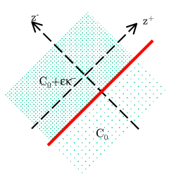
Figure 3: Shock wave solution in two–dimensional dilaton gravity.

The positivity of $\epsilon$ can be understood by looking at the conformally coupled scalar, for which $\tau_{--}=2\left(\nabla_{-}\eta\right)^{2}>0$. Recalling from (14) that

$$\nabla_{-}C=2\tau_{--}\nabla_{+}\Phi\,e^{-\Omega}=\tau_{--}\kappa^{-}\,,$$ (17)

we conclude that the shock front interpolates, as we move along $z^{-}$, between the vacuum solution with $C=C_{0}$ and the vacuum solution with $C=C_{0}+\epsilon\kappa^{-}\left(z_{0}^{-}\right)$ (see Figure 3). As a consistency check note that, since in the vacuum $\tau_{--}$ and $\kappa^{-}$ are functions only of $z^{-}$, equation (17) defines a jump in the function $C$ which is independent of the position $z^{+}$ along the shock wave.

4.2 The Case $V=2\Phi^{-3}$

We now specialize to the action (9) by taking

$$V=\frac{2}{\Phi^{3}}\,,\ \ \ \ \ \ \ \ \ \ \ \ \ \ \ \ \ \ \ \ \ \ \ \ \ \ \ \ \ \ J=-\frac{1}{\Phi^{2}}\,.$$

First consider the vacuum solutions. These are easy to obtain by considering the flat metric (2) written in the coordinates $x^{\pm}=X^{\pm}e^{\mp EY}$ and $y=\sqrt{E}Y$, where $E>0$ is a constant with units of energy,

$$\frac{\partial}{\partial y}=\sqrt{E}\left(X^{+}\partial_{+}-X^{-}\partial_{-}\right)+\frac{1}{\sqrt{E}}\,\partial_{Y}$$

is a Killing direction and $x^{\pm}$ are the two–dimensional coordinates. If one rewrites the metric in the form (7), it is easy to check the normalization (8) and to compute the two–dimensional metric and dilaton field. The explicit computation is done in [3] and the result corresponds to the cosmological solution shown in Figure 4, where the timelike orientifold singularities are at a distance of order $E^{-1}$. For future use, we divide the diagram in various regions I_in,out, II_L,R and III_L,R, as shown in the Figure.

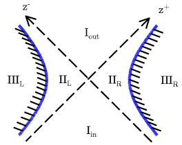
Figure 4: The cosmological vacuum solution for $V=2\Phi^{-3}$. Regions I_in, I_out are the contracting and expanding cosmologies, whereas regions II_L,R are the intermediate regions. Regions III_L,R are after the singularities, and correspond, when uplifted to three dimensions, to the regions where the Killing vector $\kappa$ becomes timelike.

Analytic results are simplest in Lorentzian polar coordinates. For example, in the Rindler wedges II_L and II_R, where $x^{+}x^{-}<0$, one uses coordinates $t,x$ defined by $x^{\pm}=\pm xe^{\pm t}$ and obtains the static solution [3]

$$ds_{2}^{2} = -dt^{2}\left(\frac{x^{2}}{1-E^{2}x^{2}}\right)+dx^{2}\,,$$ (18)

$$\Phi = \frac{1}{\sqrt{E}}\sqrt{1-E^{2}x^{2}}\,.$$

It is easy to check that the above solution satisfies (15) and (16) with

$$C=-E.$$

As we already discussed in section 3, these $C<0$ solutions correspond to non BPS $O8$–$\overline{O8}$ geometries when uplifted to string theory with equation (10). Notice that, given $E$ (or equivalently $g_{s}$ by equation (11)), one has no freedom in the solution, which is unique. Therefore, no fine tuning is required in the initial conditions for the metric and the dilaton in order to obtain a solution with a bounce and with past and future cosmological horizons. Recall also that the conformal field theory description of the $O\overline{O}$ system has two distinct moduli, which are the string coupling and the distance between the orientifolds in string units. We therefore see that the backreaction of the geometry ties the two moduli with equation (11) and reduces them to a single free parameter.

We also notice that the $C=0$ solution is clearly singled out and corresponds to the supergravity solution of a single BPS $O8$–plane. The $C>0$ solutions do not have a clear interpretation in string theory, and it would be nice to understand this point further.

Before considering more general solutions in the presence of matter, let us discuss the coordinate change from $x^{\pm}$ to conformal coordinates $z^{\pm}$. For the sake of simplicity, and since this is all we will need, we write formulae for the case $E=1$. We consider then the change of coordinates

$$z^{+}z^{-}=e^{2\Phi}\,\frac{\Phi-1}{\Phi+1},\,\ \ \ \ \ \ \ \ \ \ \ \ \ \ \ \ \ \ \ \ \ \ \ \ \frac{z^{+}}{z^{-}}=\frac{x^{+}}{x^{-}},$$ (19)

where

$$\Phi=\sqrt{x^{+}x^{-}+1}.$$

Then, it is simple to show that the metric becomes conformal

$$ds_{2}^{2}=-\frac{dz^{+}dz^{-}}{z^{+}z^{-}}\left(\frac{\Phi^{2}-1}{\Phi^{2}}\right).$$ (20)

Finally let us add matter and consider shock wave solutions. Given the discussion in section (4.1), it is now almost trivial to find the correct geometries, which are given pictorially in Figure 5. In Figure 5a, before the shock wave, we have the vacuum solution with some given value of $E$. After the wave, one has again a vacuum solution, but with a different value $E^{\prime}$. Recall that

$$E^{\prime}=E-\epsilon\kappa^{-}$$

where $\epsilon>$ $0$ and $\kappa^{-}=2\nabla_{+}\Phi\,e^{-\Omega}$ must be computed along the wave. As we move in Figure 5a from point $a$ to points $b$ and $c$ along the shock wave, in the direction of increasing $z^{+}$, the value of $\Phi$ decreases to $0$ at $c$ on the singularity. Therefore $\nabla_{+}\Phi\,<0$ and one has that

$$E^{\prime}>E.$$

Moreover, in any vacuum solution with $C=-E$, the value of the dilaton on the horizons is $1/\sqrt{E}$, as can be seen from equation (18) at $x=0$. Therefore, since the value of $\Phi$ is continuous across the shock wave, we notice that the horizon to the left of the wave, where the dilaton has value $\Phi=1/\sqrt{E^{\prime}}$, must intersect the wave between the points $b$ and $c$, as drawn.

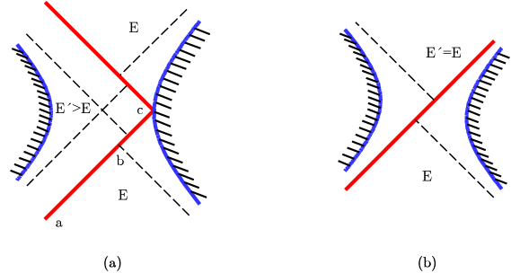
Figure 5: Shock wave solutions in the cosmological geometry.

A particular case of the shock wave geometry is attained when the wave moves along one of the horizons, as shown in Figure 5b. Since $\Phi$ is constant along the horizons, we have that $\nabla_{+}\Phi=0$ and therefore that

$$E^{\prime}=E.$$

Let us breifly explain why the horizon at a constant value of $z^{+}$ shifts as one passes the shock wave. It is easy to see that the horizon in question is given by the curve $\kappa^{+}=0$. In the vacuum, $\kappa^{+}$ is a function of $z^{+}$ alone, but in the presence of matter one has that

$$\partial_{-}\kappa^{+}=e^{-\Omega}\tau_{--}\,.$$

Then, since $\Omega$ is constant along the horizons (and therefore along the shock wave) and since $\tau_{--}$ has a delta singularity, the function $\kappa^{+}$ just jumps by a finite constant across the wave, thus explaining the shift in the position of the horizon.

Let us conclude by noticing that the instability of the null orbifold found in [11] is again a shock wave which interpolates between two different vacuum solutions. The initial solution is a BPS vacuum ($C=0$), which has a different spacetime structure from the other solutions with $C\neq 0$ which are formed after the shock wave. In our case this instability does not arise since we are interpolating between two non–BPS vacua with the same global structure.

4.3 The Shock Wave Solution in Three Dimensions

The geometry of Figure 5a corresponds, when uplifted to three dimensions, to the gravitational backreaction to matter distributed along a specific surface, which is the uplift of the shock wave curve. In order to better understand the geometry of this surface, consider first the shock wave without backreaction. From now on we take, for simplicity, $E=1$ and $E^{\prime}=1+\delta$ for some $\delta>0$. The limiting geometry for $\delta\rightarrow 0$ is given by Figure 6. The underlying 2D geometry is the vacuum $E=1$ solution, and we have singled out a specific curve, which is given, in the conformal coordinates $z^{\pm}$, by the two segments

$$z^{-} = -1\,,\ \ \ \ \ \ \ \ \ \ \ \ \ \ \ \ \ \ \ \ \ (-\infty<z^{+}<1)$$ (21)

$$z^{+} = 1\,.\ \ \ \ \ \ \ \ \ \ \ \ \ \ \ \ \ \ \ \ \ \ \ \ (-1<z^{-}<\infty)$$

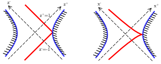
Figure 6: The shock wave before backreaction, both in conformal coordinates $z^{\pm}$ and in the coordinates $x^{\pm}$ of equation (19).

We now uplift this configuration to three dimensions. The vacuum solution becomes, as we emphasized before, nothing but flat space. The curve becomes then a specific surface in $\mathbb{M}^{3}$, whose geometry is most easily analyzed by passing to the coordinates $x^{\pm}$ in (19). It is simple to see, using the explicit coordinate transformation (19), that the curve (21) becomes (see Figure 6)

$$x^{\pm}=\left(s\pm 1\right)e^{\mp s}$$ (22)

for $s\in\mathbb{R}$. The first part of the curve (21) corresponds to (22) for $s<0$, whereas the second part corresponds to $s>0$. Comparing with (6) we immediately see that this curve corresponds, when uplifted to three dimensions, to the Horowitz–Polchinski surface $S_{1}$. Recall from section 2 that, among the various surfaces $S_{a}$, the surface $S_{1}$ is special since it is the only null surface, and it is therefore not surprising that we are obtaining exactly $S_{1}$ from the two–dimensional shock wave.

We therefore conclude that the geometry of Figure 5a, when uplifted to three dimensions, represents the gravitational backreaction to light rays distributed on the HP surface $S_{1}$.

4.4 Finding the Closed Timelike Curve

We are now in a position to investigate the existence of closed timelike curves in the geometry of Figure 5a. Recall that, without shock wave, the quotient geometry has closed timelike curves that always pass through region III, and that are removed by excising this region. These curves are not closed in the covering space, which is flat. In the geometry with the shock wave, we shall see that there are closed timelike curves already in the covering space, which could signal an instability. However these curves always pass through region III, and again should be excised.

In order to describe the closed timelike curves, we first need to prove a simple fact. Consider, in $\mathbb{M}^{3}$, two points $A$ and $B$ which are connected by a future–directed timelike curve from $A$ to $B$. Let $x_{A}^{\pm},0$ and $x_{B}^{\pm},y_{B}$ be the coordinates of these two points in the coordinate system (5) and let us assume that both points are in Region II_R, i.e. the region with $x^{+}>0$, $x^{-}<0$ and $x^{+}x^{-}<1$. We parametrize the path from $A$ to $B$ as $x^{\pm}\left(s\right),y\left(s\right)$, with $0\leq s\leq 1$. First of all, it is easy to show that the full path must be entirely regions II_R or III_R, because otherwise the horizons in the geometry prevent the curve from returning to region II_R without becoming spacelike. Therefore, since we are confined to the right Rindler wedge of the $x^{\pm}$ plane, we may adopt polar coordinates $x^{\pm}=\pm x\,e^{\pm t}$. We want to show that, if $t_{A}>t_{B}$ (the point $A$ is after the point $B$ in Rindler time), then any forward directed timelike curve from $A$ to $B$ must go into region III_R (the region with $x>1$). To prove this fact, recall first the metric on $\mathbb{M}^{3}$ in the coordinates $x,t,y$

$$dx^{2}-x^{2}dt^{2}+dy^{2}\left(1-x^{2}\right)-2x^{2}dydt\,.$$

Consider then the function $t\left(s\right)$. It starts at $t\left(0\right)=t_{A}$ and it is increasing for small values of $s$. This is because surfaces of constant $t$ are spacelike in region II_R (since $dx^{2}+dy^{2}\left(1-x^{2}\right)>0$ if $x^{2}<1$) and therefore future directed timelike curves have always $\frac{dt}{ds}>0$ in region II_R. Now, since by assumption $t_{B}<t_{A}$, the function $t\left(s\right)$ must achieve a maximum for some value of $s$. Then, using the same reasoning, the curve must be in region III_R to be timelike, and this concludes the proof. We can actually always construct a future directed timelike curve by connecting the two points $A$ and $B$ with a straight line, provided that we choose $y_{B}$ large enough, as can be seen by direct computation.

We can now prove the existence of a closed timelike curve in the full geometry (5a). The regions to the left and to the right of the wave are vacuum solutions which correspond, when uplifted to three dimensions, to regions in flat Minkowski space. We can then think of the full geometry as follows. Let $\widetilde{\mathbb{M}}^{3}$ and $\mathbb{M}^{3}$ be two copies of three–dimensional space which are going to describe the geometry to the left and to the right of the shock wave, and which we parametrize with coordinates

$$\widetilde{X}^{\pm}=\widetilde{x}^{\pm}e^{\pm\sqrt{E^{\prime}}\widetilde{y}}\,\ \ \ \ \ \ \ \ \ \widetilde{Y}=\frac{1}{\sqrt{E^{\prime}}}\ \widetilde{y}\ \ \ \ \ \ \ \ \ \ \ \ \ \ \ \ \ \ \ \ \ \ \ (\widetilde{\mathbb{M}}^{3})$$

$$X^{\pm}=x^{\pm}e^{y}\ \ \ \ \ \ \ \ \ \ \ \ \ \ \ \ Y=y\,\ \ \ \ \ \ \ \ \ \ \ \ \ \ \ \ \ \ \ \ \ \ \ \ \ \ \ \ \ \ (\mathbb{M}^{3})\$$

respectively. The shock wave itself defines surfaces $\widetilde{S}$ and $S$ in the two spaces $\widetilde{\mathbb{M}}^{3}$ and $\mathbb{M}^{3}$. The full geometry is then obtained as follows. Denote the region to the left of $\widetilde{S}$ in $\widetilde{\mathbb{M}}^{3}$ by $\widetilde{\mathbb{M}}^{3}_{L}$. This corresponds to the part of the geometry to the left of the shock wave. Similarly, denote the region to the right of ${S}$ in ${\mathbb{M}}^{3}$ by ${\mathbb{M}}^{3}_{R}$, which is the region to the right of the wave. The full geometry is then given by taking the two regions $\widetilde{\mathbb{M}}^{3}_{L}$ and ${\mathbb{M}}^{3}_{R}$ and gluing the two boundaries $\widetilde{S}$ and ${S}$ in a specific way. We do not need the details of the gluing, aside from the simple fact that $\widetilde{y}=y$ when connecting $\widetilde{S}$ and ${S}$.

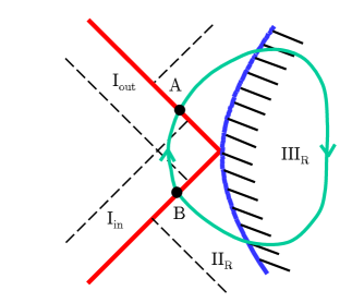
Figure 7: A closed timelike curve in the geometry induced by the surface $S_{1}$.

Looking at Figure 7, which represents the shock wave solution in conformal coordinates, choose then the two points $A$ and $B$ as drawn. They will correspond to points on the surface $\widetilde{S}$ with coordinates $\tilde{x}_{A}^{\pm},\tilde{y}_{A}$ and $\tilde{x}_{B}^{\pm},\tilde{y}_{B}$ and on $S$ with coordinates ${x}_{A}^{\pm},y_{A}$ and ${x}_{B}^{\pm},{y}_{B}$, where, as we already noticed, one has $\tilde{y}_{A}={y}_{A}$ and $\tilde{y}_{B}={y}_{B}$. As in the discussion in the previous part of this section, we choose $y_{A}=0$ and $y_{B}$ large and positive. Notice first that, with respect to the geometry ${\mathbb{M}}^{3}_{R}$ on the right of the shock wave, both points $A$ and $B$ are in region II_R, whereas they are in regions I_out and I_in relative to the geometry $\widetilde{\mathbb{M}}^{3}_{L}$ on the left of the wave. In equations, we have that

$$x_{A}^{+} > 0,\,\ \ \ \ \ \ \ \ \ x_{A}^{-}<0,\,\ \ \ \ \ \ \ \ \ x_{A}^{+}x_{A}^{-}<1,$$

$$x_{B}^{+} > 0,\,\ \ \ \ \ \ \ \ \ x_{B}^{-}<0,\,\ \ \ \ \ \ \ \ \ x_{B}^{+}x_{B}^{-}<1,\,$$

and

$$\widetilde{x}_{A}^{\pm} > 0,$$

$$\widetilde{x}_{B}^{\pm} < 0.$$

This is the key feature which is required in order to have a closed timelike curve. Let us first concentrate on the right part of the wave. We may just consider the straight line from $A$ to $B$ in ${\mathbb{M}}^{3}_{R}$ which is future directed for $y_{B}$ large, and which goes, when projected onto the $z^{\pm}$ plane as in Figure 7, in the region after the singularity. This is because the point $A$ is after point $B$ in the Rindler time of region II_R ($x^{+}_{B}/x^{-}_{B}>x^{+}_{A}/x^{-}_{A}$), and so we can apply the arguments of the first part of the section. Now we consider the region to the left of the shock wave. It is easy to check, by direct computation, that the straight segment from $B$ to $A$ in $\widetilde{\mathbb{M}}^{3}_{L}$ is still timelike for large values of $\tilde{y}_{B}=y_{B}$, and it is clearly future directed since $B$ is in I_in and $A$ is in I_out. This closes the loop, as drawn in Figure 7, and we have found a closed timelike curve.

Note that, due to the simple lemma proved above, it must be that our closed curve always goes into region III. Recall though that the boundary of region III corresponds in string theory to the orientifold $O8$–plane, and therefore region III should be excised, as described in section 3. The final $M$–theory geometry is free of closed timelike curves, and we have then shown that the presence of the orientifolds not only resolves the issues put forward in section 3, but also cures the instability due to the formation of large black holes.

4.5 Discussion

Let us conclude this section with some comments.

First of all, we can try to consider the geometry induced by light rays on surfaces $S_{a}$ for $-1<a<1$ (so that the surface does not go into region III). This corresponds, in 2D gravity, to matter which couples to the dilaton and to the conformal factor of the metric, and is therefore analytically more complex. Nonetheless, we can understand pictorially, in Figure 8, that the physics is qualitatively unaltered. In particular one can find, as before, closed timelike curves which necessarily have to pass in region III.

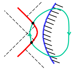
Figure 8: A closed timelike curve in the geometry induced by the surface $S_{a}$ for $a<1$.

Secondly, it is clear that, in Figure 5a, it is crucial that $E^{\prime}>E$. This fact, recall, comes from positivity requirements on the stress–energy tensor $\tau_{ab}$. If $E^{\prime}$ had been less then $E$, the graph would have had a different structure. In particular, the horizon of the left part of the geometry would have intersected the shock wave not between the points $b$ and $c$, but between $a$ and $b$. The causal structure of the space, when uplifted to three dimensions, is then quite different and it is easy to show, using arguments similar to those in the previous section, that the 3D geometry has no closed timelike curves.

Finally, let us comment on the general Horowitz–Polchinski problem for $D>3$. In this case, gravity is non–trivial even in the absence of matter, and therefore an exact solution to the problem is probably out of reach. On the other hand, it seems unlikely that a correct guess on the final qualitative features of the solution can be obtained by looking at the interaction between two (or, for that matter, a finite number) of light–rays. This fact is already true if we just consider the linear reaction of the gravitational field to the matter distributed on the HP surfaces $S_{a}$. Then, very much like in electromagnetism, it is incorrect to guess the qualitative features of fields by looking at just a finite subset of the charges (matter in this case), whenever the charge distribution is infinite (this infinity is really not an approximation in this case, since it comes from the infinite extent of the surface $S_{a}$ due to the unwrapping of the quotient space). Therefore, to decide if the problem exists in higher dimensions, much more work is required, already in the linear regime of gravity, but most importantly in the full non–linear setting. Note that the only case in which the HP argument is fully correct is exactly in dimension $D=3$, where the gravitational interaction is topological and when, therefore, the interaction of an infinite number of charges can be consistently analyzed by breaking it down into finite subsets. This indeed is what we find in the previous sections, since closed timelike curves do appear.

5 Stability of the Cosmological Cauchy Horizon

Another related classical instability which can arise in orbifold and orientifold cosmologies is due to the backreaction of general matter fields as they propagate through the bounce: as the universe contracts, particles will accelerate and will create a large backreaction in the geometry. General instabilities of this type can only be studied in the linearized regime, as opposed to the shock wave geometries which could be analyzed fully, including gravitational backreaction. In fact, in the previous section we concentrated on conformally coupled non–dilatonic matter propagating in the cosmological geometry, and this was possible due to the simple coupling to the two–dimensional gravitational fields $\Phi$ and $g_{ab}$. We now want to consider more general matter fields, either non–conformal or coupled to the dilaton. In the following, we shall concentrate on a scalar propagating in the quotient space $\mathbb{M}^{3}/e^{\kappa}$, which corresponds to a free massive scalar on the covering space $\mathbb{M}^{3}$. Our results will apply to the orientifold cosmology after imposing Dirichlet or Neumann boundary conditions on the surface $X^{+}X^{-}=-E^{2}$. These wave functions were studied in [9], and we shall review briefly those results before considering the issue of stability.

5.1 Particle States

Let us start with a massive field $\Psi$ of mass $m$ on the covering space $\mathbb{M}^{3}$, which satisfies the Klein–Gordon equation

$$\square\,\Psi(X)=m^{2}\,\Psi(X)\ .$$ (23)

We demand that $\Psi$ be invariant under the orbifold action, so that

$$\Psi(X)=\Psi(e^{\kappa}X)\ ,$$ (24)

where $\kappa=2\pi i\left(\Delta J+RK\right)$ and

$$iJ = X^{+}\partial_{+}-X^{-}\partial_{-}\ ,$$

$$iK = \partial_{Y}\ .$$

The energy scale $E$ of section 4 is given by $E=\Delta R^{-1}$. Since the quotient space has the symmetry generated by the Killing vector $\kappa$, and since the operators $J$, $K$ and $\square$ commute, it is convenient to choose a basis of solutions to (23) and (24) where the operators $J$ and $K$ are diagonal. We then choose our field $\Psi$ so that

$$J\,\Psi(X) = p\,\Psi(X)\ ,$$

$$K\,\Psi(X) = k\,\Psi(X)\ ,$$

by writing

$$\Psi_{p,k}\left(X\right)=\Psi_{p}(X^{+},X^{-})\,e^{ikY}\,.$$

The wave functions $\Psi_{p}$ are functions of Lorentzian spin $J=p$ which also satisfy the two–dimensional Klein–Gordon equation $\left(4\partial_{+}\partial_{-}+\omega^{2}\right)\Psi_{p}=0$, where $\omega^{2}=m^{2}+k^{2}$. They can then be solved in Lorentzian polar coordinates, as we shall review below, in terms of Bessel functions, which naturally have an integral representation as a sum of the standard plane waves in the covering space. In terms of the quantum numbers $p$, $k$, the orbifold boundary condition (24) becomes simply

$$\Delta\,p+\,R\,k=n\in\mathbb{Z\,}.$$ (25)

Generally, when $R\neq 0$, the spectrum of $p\in{\mathbb{R}}$ is continuous for each $n$. On the other hand, for the pure boost orbifold ($R=0$), the spectrum is discrete since $\Delta\,p=n$. This difference is crucial.  We shall see more in detail in the next section that, in the general case, it is possible to define particle states that do not destabilize the cosmological vacuum on the horizons by properly integrating over the various spins $p$, whereas in the pure boost case there is an infinite blue shift as particles approach the tip of the Minkowski cone [34]. The situation is analogous to particles propagating in the “null boost” and “null boost $+$ translation” orbifolds studied in [14]. From now on we consider the general case $R\neq 0$, and we use as quantum numbers $p$ and $n$, thus labeling the wave functions $\Psi_{p,n}$.

To study the behaviour of the wave functions describing the collapse of matter through the contracting region I_in we first move to light–cone coordinates $x^{\pm}=X^{\pm}e^{\mp EY}$ and then to polar coordinates in the Milne wedge of the $x^{\pm}$ plane $x^{\pm}=t\,e^{\pm Ex}$. This means that, using the quantization condition (25), the wave function $\Psi_{p,n}$ is given by

$$\Psi_{p,n}\left(X\right)=\Psi_{p}^{\left(\pm\right)}(x^{+},x^{-})\,e^{i\frac{n}{R}Y}\,,$$ (26)

where the functions $\Psi_{p}^{\left(\pm\right)}$ have the form

$$\Psi_{p}^{\left(\pm\right)}=J_{\pm ip}(\omega|t|)\,e^{ipEx}$$

and where $J_{\pm ip}$ are the Bessel functions of imaginary order $\pm ip$. In terms of the quantum numbers $p$ and $n$, the frequency $\omega$ satisfies the mass shell condition

$$\omega^{2}=m^{2}+\left(Ep-\frac{n}{R}\right)^{2}\ .$$

5.2 Near Horizon Behaviour of the Wave Functions

We are interested in the limit $t\rightarrow 0$ near the cosmological horizon, so it is convenient to recall the basic functional form of the Bessel functions

$$J_{\pm ip}(\omega|t|)=\left(\frac{\omega|t|}{2}\right)^{\pm ip}F_{\pm ip}\left(\omega^{2}t^{2}\right)\ ,$$

where $F_{\pm ip}$ is an entire function on the complex plane, which has the expansion

$$F_{\pm ip}(z)=\sum_{k=0}^{\infty}\frac{(-)^{k}}{4^{k}\,k!\,\Gamma(k+1\pm ip)}\,z^{k}\ .$$

Then, in terms of the two–dimensional light–cone coordinates $x^{\pm}$, which are well defined throughout the whole geometry, we have

$$\Psi_{p}^{\left(\pm\right)}=\left(\frac{\omega|x^{\pm}|}{2}\right)^{\pm ip}F_{\pm ip}\left(\omega^{2}x^{+}x^{-}\right)\ .$$

These wave functions are well behaved everywhere except at the horizons $x^{\pm}=0$, where there is an infinite blue–shift of the frequency. To see this, consider the leading behaviour of the wave function $\Psi_{p}^{(+)}$ at both horizons ($x^{+}=0$ or $x^{-}=0$)

$$\Psi_{p}^{(+)}\sim\left(\frac{\omega|x^{+}|}{2}\right)^{ip}\frac{1}{\Gamma(1+ip)}\ .$$

Near the horizon $x^{-}=0$ the wave function is well behaved and can be trivially continued through the horizon. Near $x^{+}=0$, on the other hand, the wave function has a singularity which can be problematic. In fact, close to the horizon, the derivative of the field $\partial_{+}\Psi_{p}^{(+)}\propto\left(x^{+}\right)^{ip-1}$ diverges as $x^{+}\rightarrow 0$, and this signals an infinity energy density, since the metric near the horizon has the regular form $ds^{2}\simeq-dx^{+}dx^{-}$. This fact was noted already in [34, 40].

A natural way to cure the problem is to consider wave functions which are given by linear superpositions of the above basic solutions with different values of $p$. The problem is then to understand if general perturbations in the far past $t\ll-E^{-1}$ will evolve into the future and create an infinite energy density on the horizon, thus destabilizing the geometry. This problem is well known in the physics of black holes where, generically, Cauchy horizons are unstable to small perturbations of the geometry [36, 37]. We will show in the next section that the problem does not arise in this cosmological geometry. More precisely, we will show that perturbations which are localized in the $x$ direction in the far past $t\ll-E^{-1}$ (and which are therefore necessarily a superposition of our basic solutions (26)) do not induce infinite energy densities on the horizons of the geometry, and can be continued smoothly into the other regions II_L,R and I_out of the geometry.

This problem was also considered in [54], where a different conclusion was reached. We will discuss, at the end of section 5.4, the argument of [54] and describe why it does not apply to physically relevant bounded perturbations.

5.3 Analysis of Infalling Matter

For simplicity we will set, from now on, $E=1$ and $m=0$ and we will focus uniquely on the uncharged sector $n=0$, which corresponds to pure dimensional reduction. The three–dimensional action for the massless scalar $\Psi$ reduces, in two dimensions, to

$$\int d^{2}x\sqrt{g}\Phi\left(\nabla\Psi\right)^{2}\,.$$

The scalar field $\Psi$ is therefore conformally coupled, but has a non trivial coupling to the dilaton, and satisfies the equation of motion

$$\square\Psi+\nabla\ln\Phi\cdot\nabla\Psi=0\,.$$ (27)

As in the previous section, we analyze this equation in the background described by the vacuum solution (18), which is given in regions I_in,out by

$$ds^{2} = -dt^{2}+\frac{t^{2}}{1+t^{2}}dx^{2}\,,$$ (28)

$$\Phi = \sqrt{1+t^{2}}\,,$$

where $x^{\pm}=te^{\pm x}$. We have seen, in the previous section, that the solutions to (27) are known exactly in terms of Bessel functions, since (27) is equivalent to the equation $\left(\square_{\mathrm{Flat}}-J^{2}\right)\Psi=0$, where $J=-i\frac{\partial}{\partial x}$ is the boost operator in the $x^{\pm}$ plane and $\square_{\mathrm{Flat}}$ is the Laplacian with respect to the flat metric $-dt^{2}+t^{2}dx^{2}\,$. A different and more general approach to the solution of (27), which is more in line with the literature on the stability of Cauchy horizons in black hole geometries, is to rewrite (27) in terms of the field

$$\Lambda=\Psi\sqrt{\Phi}\,.$$

A simple computation shows that equation (27) becomes

$$\square\Lambda+\frac{1}{4\Phi^{2}}\left[\left(\nabla\Phi\right)^{2}-2\Phi\square\Phi\right]\Lambda=0\,.$$

We now use the fact that, in the vacuum solution (28), equations (12) and (13) with $C=-1$ imply that $\square\Phi=-2\Phi^{-3}$ and that $\left(\nabla\Phi\right)^{2}=-1+\Phi^{-2}$. Therefore the equation of motion becomes

$$\square\Lambda+\frac{5-\Phi^{2}}{4\Phi^{4}}\Lambda=0\,.$$ (29)

As customary, we write the above equation using conformal coordinates defined in region I_in. In the sequel, we follow closely the beautiful work of Chandrasekar and Hartle [37]. We first define, in terms of the coordinates $z^{\pm}$ in (19), the coordinates $u$, $v$ given by

$$z^{+} = -e^{-v}\,,$$

$$z^{-} = -e^{-u}\,.$$

The coordinates $u$, $v$ are lightcone coordinates in the $s$, $x$ plane

$$u = s+x\,,$$

$$v = s-x\,,$$

where $s$ is the usual tortoise time coordinate. Recalling (19), $s$ is given in terms of $t$ by the expression

$$s=-\sqrt{1+t^{2}}+\frac{1}{2}\ln\frac{\sqrt{1+t^{2}}+1}{\sqrt{1+t^{2}}-1}\,$$ (30)

and has asymptotic behaviour for large values of $\left|s\right|$ given by (see Figure 9)

$$s \sim t\,,\ \ \ \ \ \ \ \ \ \ \ \ \ \ \ \ \ \ \ \ \ \ \ \ \ \ \ \ \ \ \ \ \ \ \ \ \ \ \ \ \ \ \left(s\ll-1\right)$$

$$s \sim -\ln\left(-t\right)\,.\ \ \ \ \ \ \ \ \ \ \ \ \ \ \ \ \ \ \ \ \ \ \ \ \ \ \ \ \ \ \ \left(s\gg 1\right)$$

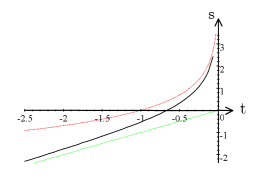
Figure 9: The tortoise time coordinate $s$ versus $t$, together with the asymptotic behaviours $t$ and $-\ln(-t)$ for $t\to-\infty$ and $t\sim 0$.

The various coordinate systems are recalled in Figure 12a. The metric in region I_in is given, from equation (20), by $-dudv\,t^{2}\left(1+t^{2}\right)^{-1}$, and we conclude that equation (29) reads

$$\left(\frac{\partial^{2}}{\partial s^{2}}-\frac{\partial^{2}}{\partial x^{2}}\right)\Lambda\left(s,x\right)=V\left(s\right)\Lambda\left(s,x\right)\,,$$

where

$$V=\frac{t^{2}}{4}\frac{\left(4-t^{2}\right)}{\left(1+t^{2}\right)^{3}}\,.$$ (31)

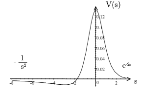
Figure 10: The scattering potential $V(s)$.

Finally, we Fourier transform the $x$ coordinate

$$\Lambda\left(s,x\right)=\int dp\,e^{ipx}\,\Lambda\left(s,p\right)$$

to obtain the Schrödinger–like equation

$$\left(\frac{\partial^{2}}{\partial s^{2}}+p^{2}\right)\Lambda\left(s,p\right)=V\left(s\right)\Lambda\left(s,p\right)\,.$$ (32)

Let us consider this differential equation in more detail. The potential $V\left(s\right)$, shown in Figure 10, has the following asymptotic behaviour

$$V \sim e^{-2s}\,\,,\ \ \ \ \ \ \ \ \ \ \ \ \ \ \ \ \ \ \ \ \ \ \ \ \ \ \ \ \ \ \ \ \ \ \ \ \ \ \ \ \ \ \ \ \ \left(s\rightarrow\infty\right)$$ (33)

$$V \sim -\frac{1}{4s^{2}}\,\ ,\ \ \ \ \ \ \ \ \ \ \ \ \ \ \ \ \ \ \ \ \ \ \ \ \ \ \ \ \ \ \ \ \ \ \ \ \ \ \ \ \left(s\rightarrow-\infty\right)$$

and is therefore significant only in the region around $s\sim 0$. The scattering potential connects the two regions with $s\ll-1$ and $s\gg 1$ (or $t\ll-1$ and $t\sim 0$) where the field $\Lambda$ behaves essentially like a free scalar in two–dimensional flat space. The potential $V$ then connects the past Minkowski region ($t\ll-1$ with metric $-dt^{2}+dx^{2}$) to the future Milne wedge ($t\sim 0$ with metric $-dt^{2}+t^{2}dx^{2}$). Since $V$ decays at infinity faster then $s^{-1}$, one can follow the usual theory of one–dimensional scattering. In particular, following [37], we consider the solutions $F\left(s,p\right)$ and $P\left(s,p\right)$ of (32) which behave like pure exponentials $e^{-ips}$ respectively in the future $s\rightarrow\infty$ and in the past $s\rightarrow-\infty$

$$F\left(s,p\right) \sim e^{-ips}\sim\left(-t\right)^{ip}\,,\,\ \ \ \ \ \ \ \ \ \ \ \ \ \ \ \ \ \ \ \ \ \ \ \ \left(s\rightarrow\infty\right)$$ (34)

$$P\left(s,p\right) \sim e^{-ips}\sim e^{-ipt}\,.\ \ \ \ \ \ \ \ \ \ \ \ \ \ \ \ \ \ \ \ \ \ \ \ \ \ \ \left(s\rightarrow-\infty\right)$$

Therefore, when restoring the $x$ dependence $e^{ipx}$ of the full solution, we have, for $s\to\infty$, the plane waves

$$e^{ipx}F\left(s,p\right) \sim e^{-ipv}\,,$$

$$e^{ipx}F\left(s,-p\right) \sim e^{ipu}\,,$$

and, for $s\to-\infty$,

$$e^{ipx}P\left(s,p\right) \sim e^{-ipv}\,,$$

$$e^{ipx}P\left(s,-p\right) \sim e^{ipu}\,.$$

As explained in the previous section, the problem is exactly soluble in terms of Bessel functions, and one has the following explicit form of the functions $F$ and $P$

$$F\left(s,p\right) = \left(\frac{2}{p}\right)^{ip}\,\Gamma\left(1+ip\right)\,\,J_{ip}\left(-pt\right)\,\left(1+t^{2}\right)^{\frac{1}{4}}\,,$$

$$P\left(s,p\right) = e^{\frac{i\pi}{4}-\frac{\pi p}{2}}\,\sqrt{\frac{\pi p}{2}}\,H_{ip}^{\left(1\right)}\left(-pt\right)\,\left(1+t^{2}\right)^{\frac{1}{4}}\,,$$

where $t=t\left(s\right)$ is defined by (30). The function

$$H_{ip}^{\left(1\right)}=\frac{1}{\sinh\left(\pi p\right)}\left(e^{\pi p}J_{ip}-J_{-ip}\right)$$ (35)

is the Hankel function of the first kind, which has the correct asymptotic behaviour to ensure that $P(s,p)$ has the desired properties.

It is useful, again following closely [37], to consider the general analytic behaviour of $F$ and $P$ as a function of the complex variable $p$, at fixed time $s$. First it is clear that we must have

$$\overline{F\left(s,p\right)} = F\left(s,-\overline{p}\right)\,,$$

$$\overline{P\left(s,p\right)} = P\left(s,-\overline{p}\right)\,.$$

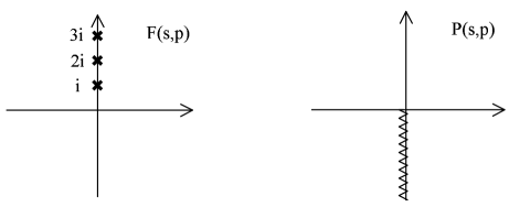
Figure 11: The analytic structure of $F(s,p)$ and $P(s,p)$ as functions of $p$.

Moreover, we recall from [37] that, whenever the potential has asymptotic behaviour

$$V \sim e^{-2\kappa_{-}s}\,,\ \ \ \ \ \ \ \ \ \ \ \ \ \ \ \ \ \ \ \ \ \ \ \ \ \ \ \ \ \ \ \ \ \ \ \left(s\rightarrow\infty\right)$$

$$V \sim e^{2\kappa_{+}s}\ ,\ \ \ \ \ \ \ \ \ \ \ \ \ \ \ \ \ \ \ \ \ \ \ \ \ \ \ \ \ \ \ \ \ \ \ \ \left(s\rightarrow-\infty\right)$$

then $F\left(s,p\right)$ is everywhere analytic, except for poles at $p=i\kappa_{-}\,\mathbb{N}\$(with $\mathbb{N}$ being the natural numbers $1,2,\cdots$), and $P\left(s,p\right)$ has poles at $p=-i\kappa_{+}\mathbb{N}$. In our case $\kappa_{-}=1$ and, as expected, the function $F$ has poles at $p=i\mathbb{N}$ due to the gamma function $\Gamma\left(1+ip\right)$. On the other hand, for the case of the specific potential (31), one has $\kappa_{+}\rightarrow 0$, with the exponential behaviour replaced with a power law $s^{-2}$. This is a direct consequence of the fact that the metric distance from a point in region I_in to the horizon at $s\rightarrow\infty$ is finite, whereas it is infinite going to past infinity at $s\rightarrow-\infty$. Therefore, the poles at $-i\kappa_{+}\mathbb{N}$ become infinitely close and are effectively replaced by a branch cut along the negative imaginary $p$ axis, as one can check from the analytic expression for $P$. The features just described, which are shown in Figure 11, are generic and do not depend on the details of the potential, but only on the asymptotic behaviour (33). In particular, one has the same behaviour for fluctuations of any field.

Let us now consider a general solution $\Lambda\left(s,p\right)$ of (32). Since both $F\left(s,\pm p\right)$ and $P\left(s,\pm p\right)$ are bases of the solutions of (32), one must have that

$$\Lambda\left(s,p\right) = V_{F}\left(p\right)F\left(s,p\right)+U_{F}\left(p\right)F\left(s,-p\right)$$ (36)

$$= V_{P}\left(p\right)P\left(s,p\right)+U_{P}\left(p\right)P\left(s,-p\right)\,.$$

The coefficients $V_{F,P}$ and $U_{F,P}$ can be easily computed by recalling that, given two solutions $f$, $g$ of (32), the Wronskian

$$\left[f,g\right]=f\dot{g}-g\dot{f}$$

is independent of $s$, where the dot denotes differentiation with respect to $s$.

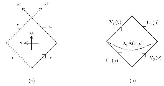
Figure 12: Figure (a) shows the various coordinate systems in region I_in. Figure (b) shows the various ways to define a solution $\Lambda$. One either gives the functions $V_{P}$, $U_{P}$ or the functions $V_{F}$, $U_{F}$, or, alternatively, the functions $\Lambda(s_{0},x)$, $\dot{\Lambda}(s_{0},x)$ at some fixed time $s_{0}$ along the dotted line.

In particular, one can easily show that

$$\left[F\left(s,p\right),F\left(s,-p\right)\right]=\left[P\left(s,p\right),P\left(s,-p\right)\right]=2ip\,.$$

Therefore we readily conclude that

$$V_{F}\left(p\right) = \frac{1}{2ip}\left[\Lambda\left(s,p\right),F\left(s,-p\right)\right]\,,$$ (37)

$$U_{F}\left(p\right) = -\frac{1}{2ip}\left[\Lambda\left(s,p\right),F\left(s,p\right)\right]\,,$$

together with similar equations for $V_{P}$ and $U_{P}$.

5.4 Behaviour at the Horizons

The meaning of the coefficients $V_{F}$ and $U_{F}$ is quite clearly understood by considering the value of the field $\Lambda$ on the horizons. Since we are in the limit $s\rightarrow\infty$, we use the asymptotic form of $F\left(s,p\right)$ to conclude that (see Figure 12b)

$$\Lambda\left(v,u\right)\rightarrow V_{F}\left(v\right)+U_{F}\left(u\right)\,,$$ (38)

where

$$V_{F}\left(v\right)=\int dp\,V_{F}\left(p\right)e^{-ipv}\,,\ \ \ \ \ \ \ \ \ \ \ \ \ \ \ U_{F}\left(u\right)=\int dp\,U_{F}\left(p\right)e^{ipu}\,.$$

To compute the stress tensor due to the fluctuation in $\Lambda$, whose divergence usually signals the instability of the Cauchy horizon, we also must consider the derivatives of the field with respect to the coordinates $z^{\pm}$ (the coordinates $u$, $v$ tend to $\infty$ on the horizons). Recalling that

$$\partial_{+}=-e^{v}\partial_{v}\,,\ \ \ \ \ \ \ \ \ \ \ \ \ \ \ \ \ \ \ \ \ \ \ \ \ \ \ \ \ \ \ \ \ \ \partial_{-}=-e^{u}\partial_{u}\,,$$

we conclude that

$$\partial_{+}\Lambda\left(v,u\right) \rightarrow -e^{v}\partial_{v}V_{F}\left(v\right)\,,$$ (39)

$$\partial_{-}\Lambda\left(v,u\right) \rightarrow -e^{u}\partial_{u}U_{F}\left(u\right)\,.$$

Note that both expressions (38) and (39) are valid only in the limit $(u\rightarrow\infty\mathit{,\ }$ $v\mathit{\ }\mathrm{fixed})$ or $\left(v\rightarrow\infty\mathit{,\ }u\mathit{\ }\mathrm{fixed}\right)$, and are not approximate expressions for large but finite $u$, $v$. This is because, although the asymptotic form (34) is exactly valid in the limit $s\rightarrow\infty$, it becomes accurate for $s\gg\overline{s}\left(p\right)$, where the threshold value $\overline{s}\left(p\right)$ depends explicitly on $p$. Given the explicit form of $F$, it is clear that $\overline{s}\left(p\right)\sim\ln p$ since only in this case is the argument of the Bessel function $-pt\ll 1$. Therefore, given a function $\Lambda$ which has support at all momenta, one is not uniformly in the asymptotic region for all momenta at any large but finite $s$. Only in the limit $s\rightarrow\infty$ we can use uniform convergence to deduce the expressions (38) and (39), in the sense just described.

Finally, going back to the computation of the derivatives $\partial_{\pm}\Lambda$, one recalls from [37] that the problematic limits are given by $\lim_{v\rightarrow\infty}\,\partial_{+}\Lambda$ and $\lim_{u\rightarrow\infty}\,\partial_{-}\Lambda$. Concentrating on the first one for simplicity, we see that we need to consider the expression

$$\lim_{v\rightarrow\infty}\,\partial_{+}\Lambda = \lim_{v\rightarrow\infty}\,e^{v}\int dp\,V_{F}\left(p\right)\,ip\,e^{-ipv}$$

$$= \frac{1}{2}\lim_{v\rightarrow\infty}\,e^{v}\int dp\left[\Lambda\left(s,p\right),F\left(s,-p\right)\right]\,e^{-ipv}\,.$$

The physical problem we need to address is the following. Let us assume that, at some time $s_{0}\ll 0$ in the past, much before the scattering potential $V\left(s\right)$ becomes relevant, our field $\Lambda$ is in some specific configuration given by initial conditions on the value of $\Lambda$ and of its time derivative $\dot{\Lambda}$

$$\Lambda\left(s_{0},x\right)\,,\ \ \ \ \ \ \ \ \ \ \ \ \ \ \ \ \ \ \ \ \ \ \ \dot{\Lambda}\left(s_{0},x\right)\,.$$

We will assume that the functions above are localized as a function of $x$. More precisely, we shall demand that $\Lambda\left(s_{0},x\right)$ and $\dot{\Lambda}\left(s_{0},x\right)$ are such that their evolution would not lead to an inconsistent behaviour on the horizon in the Milne wedge of flat space, where $V=0$. It is important to realize that those are the general physical perturbation, since we are only demanding that they would be regular in flat space. Let us be more explicit. In the absence of the potential $V$, the solutions of the massless Klein–Gordon equations are just $\Lambda=\alpha(v)+\beta(u)$, and the initial conditions $\Lambda$ and $\dot{\Lambda}$ at $s_{0}$ are equivalent to giving the functions $\alpha$ and $\beta$ of the light–cone coordinates. Recall though that the coordinates which are regular across the horizon are $z^{\pm}$, and therefore we must demand, in order to have a regular perturbation in flat space, that $\alpha$ and $\beta$ be well–behaved as functions of $z^{\pm}$. To see what this means in practice, consider a function of $z^{+}$ which has a nice power series expansion $a_{0}+a_{1}z^{+}+\cdots$ around $z^{+}=0$. As a function of $v$ this reads $\alpha(v)=a_{0}-a_{1}e^{-v}+\cdots$, and this shows that, aside from the constant part, the function $\alpha(v)$ must decay, for $v\to\infty$, at least as fast as $e^{-v}$. This fact imposes constraints on the Fourier transforms of $\alpha$ and $\beta$ and, in turn, on the functions $\Lambda(s_{0},x)$ and $\dot{\Lambda}(s_{0},x)$. In practice, it is sufficient to require that the Fourier transforms $\Lambda\left(s_{0},p\right)$ and $\dot{\Lambda}\left(s_{0},p\right)$ do not have poles in the strip $\left|\mathop{\mathrm{I}m}p\right|<1$. Then the problematic limit

$$\frac{1}{2}\lim_{v\rightarrow\infty}\,e^{v}\int dp\left[\Lambda\left(s_{0},p\right)\dot{F}\left(s_{0},-p\right)-\dot{\Lambda}\left(s_{0},p\right)F\left(s_{0},-p\right)\right]\,e^{-ipv}$$

can be computed by deforming the contour in the lower half of the complex plane, and is determined by the poles of $F\left(s,-p\right)$. In fact, the leading behaviour of the integral is controlled by the first pole at $-i$, which gives an asymptotic behaviour for large $v\rightarrow\infty$ of $e^{-v}$. The limit in the above expression then tends to a finite result.

In order to better understand the above result, let us review the standard argument for the instability of the Cauchy horizon, which was followed in [54]. The problem is usually posed by giving initial conditions at past null infinity (see also Figure 12b), by giving the functions

$$V_{P}\left(v\right)=\int dp\,V_{P}\left(p\right)e^{-ipv}\,,\ \ \ \ \ \ \ \ \ \ \ \ \ \ \ \ U_{P}\left(u\right)=\int dp\,U_{P}\left(p\right)e^{ipu}\,,$$

on which we impose a regularity constraint (say, for simplicity, a localization condition like the one discussed above, now in the coordinates $v$ and $u$). To determine $V_{F}$, $U_{F}$ in terms of $V_{P}$, $U_{P}$ one uses the expression (36) for $\Lambda$ in the equation (37) and obtains that

$$\left(\begin{array}[]{c}V_{F}\left(p\right)\\ U_{F}\left(p\right)\end{array}\right)=\left(\begin{array}[]{cc}A\left(p\right)&B\left(-p\right)\\ B\left(p\right)&A\left(-p\right)\end{array}\right)\left(\begin{array}[]{c}V_{P}\left(p\right)\\ U_{P}\left(p\right)\end{array}\right)\,,$$

where

$$A\left(p\right) = \frac{1}{2ip}\left[P\left(s,p\right),F\left(s,-p\right)\right]\,,$$

$$B\left(p\right) = -\frac{1}{2ip}\left[P\left(s,p\right),F\left(s,p\right)\right]\,.$$

The above expression shows that both $A\left(p\right)$ and $B\left(p\right)$ have a cut along the negative imaginary $p$ axis (the limit of the poles at $-i\kappa_{+}n$ for $\kappa_{+}\rightarrow 0$). The full analytic structure of $A(p)$ and $B(p)$ is shown in Figure 13. Since $V_{F}\left(p\right)=V_{P}\left(p\right)A\left(p\right)+U_{P}\left(p\right)B\left(-p\right)$ we conclude that the leading pole of $V_{P}(p)A(p)$ at $-i\kappa_{+}\rightarrow-i0$ determines the asymptotic behaviour of the integral in (5.4) to be $e^{-\kappa_{+}v}$. Therefore, the limit $\lim_{v\rightarrow\infty}e^{v\left(1-\kappa_{+}\right)}$ diverges, thus naively signaling an instability of the horizon.

Figure 13: The analytic structure of $A(p)$ and $B(p)$.

The above reasoning depends crucially on the assumption that the functions $U_{P}$, $V_{P}$ have a nice Fourier transform (analytic at least in the region $\left|\mathop{\mathrm{I}m}p\right|<1$), so that the perturbation is localized on the null directions at past null infinity. If this is the case, though, expression (36) shows that the function $\Lambda\left(s,x\right)$ is already delocalized (the Fourier transform has a branch cut due to $P\left(s,p\right)$) at any finite time $s\ll-1$ much before the scattering potential, and therefore will concentrate on the horizons and create an infinite stress tensor. This is clearly not the type of perturbation we want to focus on, which should be localized in space before they hit the potential $V$. Note that, at any finite time $s$, we cannot use, in equation (36), the asymptotic form of $P(s,p)$ for all values of $p$. In fact, the explicit form of the the function $P$ shows that one is in the asymptotic regime for $|p|\gg s^{-1}$. Therefore, the crucial low momentum modes which determine the asymptotic behaviour of the wave function are never in the asymptotic region for any finite time $s$. We then consider the requirement of localization of $\Lambda\left(s,x\right)$ at times $s\ll-1$ to be the correct and physically relevant boundary condition to study issues of stability of the geometry. The reasonings of this section then show that, in this sense, the Cauchy horizon in perfectly stable to small perturbations.

5.5 Discussion

Let us conclude this section with some comments on future research.

We have shown that, in the orientifold cosmology, one can define particle–like perturbations which do not destabilize the Cauchy horizon, and therefore that the solution is stable against small variations of the background fields. All the work is done at the classical linearized level. The most pressing question for issues of stability is the study of the quantum stress–energy tensor for the field $\Psi$. This is a non–trivial problem due to the non–minimal coupling to the metric and the dilaton, and only some results are known in the literature (see [50, 51] and references therein). On the other hand, the problem might be tractable since the exact wave–functions are known in this case.

6 Conclusion

In this paper we investigate the classical stability of a two–dimensional orientifold cosmology, related to a time–dependent orbifold of flat space–time. We saw, with a specific counter example, that the instability argument of Horowitz and Polchinski is not valid once the time–like orbifold singularity is interpreted as the boundary of space–time. In this specific example, we consider an exact shock–wave solution of two–dimensional dilaton gravity that uplifts to a distribution of matter in the three–dimensional covering space. According to Horowitz and Polchinski this distribution should interact gravitationally creating large black holes. Indeed, there are closed time–like curves in the covering space geometry of the shock–wave, signaling the three–dimensional gravitational instability. However, such CTC’s are not present if we interpret the singularity as a boundary of space–time, and accordingly excise from the geometry the region behind it.

The other stability problem addressed in this work is related to cosmic censorship. The presence of naked singularities with a Cauchy Horizon has lead many people to believe that such singularities never form. Indeed, as for the Reissner–Nordstrom black hole one expects the Cauchy horizon to be unstable when crossed by matter. We analyze the propagation of a scalar field coupled to gravity in the geometry, and show that any localized fluctuation at some finite time in the far past will not destabilize the horizon. The existence of the time–like singularity does not imply the break–down of predictability because of the conjectured duality between the singularity and orientifolds of string theory. To leading approximation, the effect of the orientifolds is to enforce a boundary condition on the fields, which determines uniquely their evolution. A more complete quantum understanding of this system is desirable.

References

-
[1]
J. Khoury, B. A. Ovrut, N. Seiberg, P. J. Steinhardt and N. Turok,
From big crunch to big bang,
hep-th/0108187.
N. Seiberg, From big crunch to big bang - is it possible?, hep-th/0201039. - [2] V. Balasubramanian, S. F. Hassan, E. Keski-Vakkuri and A. Naqvi, A space-time orbifold: A toy model for a cosmological singularity, hep-th/0202187.
- [3] L. Cornalba and M. S. Costa, A New Cosmological Scenario in String Theory, Phys. Rev. D 66 (2002) 066001, hep-th/0203031.
- [4] N. A. Nekrasov, Milne universe, tachyons, and quantum group, hep-th/0203112.
- [5] J. Simon, The geometry of null rotation identifications, hep-th/0203201.
- [6] A. J. Tolley and N. Turok, Quantum fields in a big crunch / big bang spacetime, Phys. Rev. D 66 (2002) 106005, hep-th/0204091.
- [7] H. Liu, G. Moore and N. Seiberg, Strings in a time-dependent orbifold, JHEP 0206 (2002) 045, hep-th/0204168.
- [8] S. Elitzur, A. Giveon, D. Kutasov and E. Rabinovici, From big bang to big crunch and beyond, JHEP 0206 (2002) 017, hep-th/0204189.
- [9] L. Cornalba, M. S. Costa and C. Kounnas, A resolution of the cosmological singularity with orientifolds, Nucl. Phys. B 637 (2002) 378, hep-th/0204261.
- [10] B. Craps, D. Kutasov and G. Rajesh, String propagation in the presence of cosmological singularities, JHEP 0206 (2002) 053, hep-th/0205101.
- [11] A. Lawrence, On the instability of 3D null singularities, JHEP 0211 (2002) 019, hep-th/0205288.
- [12] C. Gordon and N. Turok, Cosmological perturbations through a general relativistic bounce, hep-th/0206138.
- [13] E. J. Martinec and W. McElgin, Exciting AdS orbifolds, JHEP 0210 (2002) 050, hep-th/0206175.
- [14] H. Liu, G. Moore and N. Seiberg, Strings in time-dependent orbifolds, JHEP 0210 (2002) 031, hep-th/0206182.
- [15] M. Fabinger and J. McGreevy, On smooth time-dependent orbifolds and null singularities, hep-th/0206196.
- [16] G. T. Horowitz and J. Polchinski, Instability of spacelike and null orbifold singularities, Phys. Rev. D 66 (2002) 103512, hep-th/0206228.
- [17] A. Buchel, P. Langfelder and J. Walcher, On time-dependent backgrounds in supergravity and string theory, Phys. Rev. D 67 (2003) 024011, hep-th/0207214.
- [18] S. Hemming, E. Keski-Vakkuri and P. Kraus, Strings in the extended BTZ spacetime, JHEP 0210 (2002) 006, hep-th/0208003.
- [19] J. Figueroa-O’Farrill and J. Simon, Supersymmetric Kaluza-Klein reductions of M2 and M5 branes, hep-th/0208107.
- [20] A. Hashimoto and S. Sethi, Holography and string dynamics in time-dependent backgrounds, Phys. Rev. Lett. 89 (2002) 261601, hep-th/0208126.
- [21] J. Simon, Null orbifolds in AdS, time dependence and holography, JHEP 0210 (2002) 036, hep-th/0208165.
- [22] M. Alishahiha and S. Parvizi, Branes in time-dependent backgrounds and AdS/CFT correspondence, JHEP 0210 (2002) 047, hep-th/0208187.
- [23] E. Dudas, J. Mourad and C. Timirgaziu, Time and space dependent backgrounds from nonsupersymmetric strings, hep-th/0209176.
- [24] Y. Satoh and J. Troost, Massless BTZ black holes in minisuperspace, JHEP 0211 (2002) 042, hep-th/0209195.
- [25] L. Dolan and C. R. Nappi, Noncommutativity in a time-dependent background, Phys. Lett. B 551 (2003) 369, hep-th/0210030.
- [26] R. G. Cai, J. X. Lu and N. Ohta, NCOS and D-branes in time-dependent backgrounds, Phys. Lett. B 551 (2003) 178, hep-th/0210206.
- [27] C. Bachas and C. Hull, Null brane intersections, JHEP 0212 (2002) 035, hep-th/0210269.
- [28] R. C. Myers and D. J. Winters, From D - anti-D pairs to branes in motion, JHEP 0212 (2002) 061, hep-th/0211042.
- [29] K. Okuyama, D-branes on the null-brane, hep-th/0211218.
- [30] T. Friedmann and H. Verlinde, Schwinger meets Kaluza-Klein, hep-th/0212163.
- [31] M. Berkooz, B. Craps, D. Kutasov and G. Rajesh, Comments on cosmological singularities in string theory, hep-th/0212215.
- [32] M. Fabinger and S. Hellerman, Stringy resolutions of null singularities, hep-th/0212223.
- [33] S. Elitzur, A. Giveon and E. Rabinovici, Removing singularities, JHEP 0301 (2003) 017, hep-th/0212242.
- [34] G. T. Horowitz and A. R. Steif, Singular String Solutions With Nonsingular Initial Data, Phys. Lett. B 258 (1991) 91.
- [35] J. Figueroa-O’Farrill and J. Simon, Generalized supersymmetric fluxbranes, JHEP 0112 (2001) 011, hep-th/0110170.
- [36] M. Simpson and R. Penrose, Internal Instability in a Reissner-Nordstrom Black Hole, Int. Journ. Theor. Physics 7 (1973) 183.
- [37] S. Chandrasekhar and J.B. Hartle, On Crossing the Cauchy Horizon of a Reissner–Nordstrom Black–Hole, Proc. R. Soc. Lond. A 384 (1982) 301-315.
- [38] C. Kounnas and D. Lust, Cosmological string backgrounds from gauged WZW models, Phys. Lett. B 289 (1992) 56, hep-th/9205046.
- [39] C. Grojean, F. Quevedo, G. Tasinato and I. Zavala, Branes on charged dilatonic backgrounds: Self-tuning, Lorentz violations and cosmology, JHEP 0108 (2001) 005, hep-th/0106120.
- [40] C. P. Burgess, F. Quevedo, S. J. Rey, G. Tasinato and I. Zavala, Cosmological spacetimes from negative tension brane backgrounds, JHEP 0210 (2002) 028, hep-th/0207104.
- [41] H. J. Matschull, Black hole creation in 2+1-dimensions, Class. Quant. Grav. 16 (1999) 1069, gr-qc/9809087.
- [42] C. G. Callan, S. B. Giddings, J. A. Harvey and A. Strominger, Evanescent Black Holes, Phys. Rev. D 45 (1992) 1005, hep-th/9111056.
- [43] J. R. Gott, Closed Timelike Curves Produced By Pairs Of Moving Cosmic Strings: Exact Solutions, Phys. Rev. Lett. 66 (1991) 1126.
- [44] S. Deser, R. Jackiw and G. ’t Hooft, Physical cosmic strings do not generate closed timelike curves, Phys. Rev. Lett. 68 (1992) 267.
- [45] D. N. Kabat, Conditions For The Existence Of Closed Timelike Curves In (2+1) Gravity, Phys. Rev. D 46 (1992) 2720.
- [46] M. P. Headrick and J. R. Gott, (2+1)-Dimensional Space-Times Containing Closed Timelike Curves, Phys. Rev. D 50 (1994) 7244.
- [47] M. Banados, C. Teitelboim and J. Zanelli, The Black Hole In Three-Dimensional Space-Time, Phys. Rev. Lett. 69 (1992) 1849, hep-th/9204099.
- [48] I. Antoniadis, E. Dudas and A. Sagnotti, Supersymmetry breaking, open strings and M-theory, Nucl. Phys. B 544 (1999) 469, hep-th/9807011.
- [49] S. Kachru, J. Kumar and E. Silverstein, Orientifolds, RG flows, and closed string tachyons, Class. Quant. Grav. 17 (2000) 1139, hep-th/9907038.
- [50] S. Nojiri and S. D. Odintsov, Quantum dilatonic gravity in d = 2, 4 and 5 dimensions, Int. J. Mod. Phys. A 16, 1015 (2001), hep-th/0009202.
- [51] D. Grumiller, W. Kummer and D. V. Vassilevich, Dilaton gravity in two dimensions, Phys. Rept. 369 (2002) 327, hep-th/0204253.
- [52] D. Louis-Martinez and G. Kunstatter, On Birckhoff’s theorem in 2-D dilaton gravity, Phys. Rev. D 49 (1994) 5227.
- [53] A. R. Steif, The Quantum Stress Tensor In The Three-Dimensional Black Hole, Phys. Rev. D 49 (1994) 585, gr-qc/9308032.
- [54] C. P. Burgess, P. Martineau, F. Quevedo, G. Tasinato and I. Zavala C., Instabilities and particle production in S-brane geometries, hep-th/0301122.