Thermodynamic and gravitational instability on hyperbolic spaces

Abstract

We study the properties of anti–de Sitter black holes with a Gauss-Bonnet term for various horizon topologies ($k=0,\,\pm 1$) and for various dimensions, with emphasis on the less well understood $k=-1$ solution. We find that the zero temperature (and zero energy density) extremal states are the local minima of the energy for AdS black holes with hyperbolic event horizons. The hyperbolic AdS black hole may be stable thermodynamically if the background is defined by an extremal solution and the extremal entropy is non-negative. We also investigate the gravitational stability of AdS spacetimes of dimensions $D>4$ against linear perturbations and find that the extremal states are still the local minima of the energy. For a spherically symmetric AdS black hole solution, the gravitational potential is positive and bounded, with or without the Gauss-Bonnet type corrections, while, when $k=-1$, a small Gauss-Bonnet coupling, namely, $\alpha\ll{l}^{2}$ (where $l$ is the curvature radius of AdS space), is found useful to keep the potential bounded from below, as required for stability of the extremal background.

I Introduction

In parallel with the development of AdS conformal field theory (CFT) correspondence Maldacena97a ; Witten98 ), black holes in AdS space are known to play an important role in dual field theory Witten98a . It has also been learned that the Einstein equations when supplemented by a negative cosmological constant admit black holes as exact vacuum solutions, whose event horizons are hypersurfaces ${\cal M}$ with zero, positive or negative constant curvature ($k=0,\,+1$, or $-1$). This ${\cal M}$ may be related to the ${\cal M}^{\prime}$ on which the dual field theory is defined by a rescaling of the metric.

Anti–de Sitter black holes with nonspherical event horizons have been constructed in four and higher dimensions Vanzo ; Birmingham98a ; Mann96a . Earlier work on closely related AdS thermodynamics can be found in Lemos95a . The analysis in Birmingham98a is well motivated from the AdS/CFT correspondence. Reference Emparan99b discusses AdS/CFT duals of $k=-1$ topological black holes in the spirit of a holographic counterterm method developed in Vijay99a ; Emparan99a . Here we study the thermodynamic and gravitational stability of a class of Gauss-Bonnet (GB) black holes in AdS space, which also have the feature that the horizon (hypersurface) ${\cal M}$ is an $(n-1)$-dimensional Einstein space with constant curvature ($k=-1,\,0,\,+1$).

There is the issue of the positivity of the total energy when AdS black holes have non-spherical horizons. Usually, the positive energy theorems show a stability of spacetimes which become asymptotically either locally flat or anti–de Sitter. The known theorems do not extend to the Horowitz-Myers soliton Horowitz98a , whose AdS asymptotic is a toroidal space with a zero constant curvature. The AdS soliton is a nonsupersymmetric background but in the AdS/CFT context it is conjectured to be a ground state for planar black holes; see also Ref. Galloway01a .

Another interesting issue with hyperbolic AdS black hole spacetimes is the choice of a background. In a gravitational theory, it is necessary to make a Euclideanized action finite by assigning classically stable lowest energy configurations to AdS black hole spacetimes with a curvature $k=0,\,\pm 1$ of the horizons. For $k=+1$, the background is simply a global AdS space, which is the solution at finite temperature Hawking83a ; Witten98a . But, for $k=-1$, the ground state may be different from a solution that is locally isometric to a pure (global) AdS space Vanzo ; Birmingham98a .

Hyperbolic AdS black holes are known to exhibit some new and interesting features, such as an increase in the entropy that is not accompanied by an increment in the energy Emparan99b ; Emparan99a . They are also relevant to studying CFTs with less than maximal (or no) supersymmetry Emparan98a ; Klemm99a . In supergravity theories, maximally symmetric hyperbolic spaces naturally arise as the near-horizon region of certain $p$-branes Kehagias00a and black hole geometries Horowitz91a . Thus the choice of a ground state for the hyperbolic AdS black holes as well as their thermodynamic and gravitational (or dynamical) stability are the important issues.

For a spherically symmetric solution (i.e., $k=+1$), for instant, the AdS Schwarzschild solution, the hypersurface ${\cal M}$ is usually a round sphere, while, for hyperbolic AdS black holes, ${\cal M}$ is either a hyperbolic space $H^{n-1}$ or its quotient $H^{n-1}/\Gamma$. Therefore, for $k=-1$, one reasonably assigns the zero temperature (and zero energy) extremal state as a background; see, for example, Refs. Vanzo ; Birmingham98a . In this paper, we further show, with or without a Gauss-Bonnet term, that the extremal states are local minima of the energy for hyperbolic AdS black holes.

In Ref. Gibbons02a , Gibbon and Hartnoll studied a classical instability of spacetimes of dimensions $D>4$ against metric perturbation, by considering generalized black hole metrics in Einstein gravity. In this paper, we generalize those results by including a Gauss-Bonnet term. We find that the black hole spacetime whose AdS asymptotic is a hypersurface of negative constant curvature could be unstable under metric perturbations if the background is a zero mass topological black hole. We show that, with or without a Gauss-Bonnet term, the extremal states are local minima of the energy for $k=-1$ AdS spacetimes against linear perturbations. We further argue that the extremal background, defined with a negative extremal mass, can be gravitationally (or dynamically) stable if the ground state metric receives higher curvature corrections, like a GB term, with small couplings.

The layout of the paper is as follows. In Sec. II we give black hole solutions in AdS space, compute extremal parameters, and define different reference backgrounds in Einstein gravity modified with a Gauss-Bonnet term. In Sec. III we compute Euclideanized actions applicable to the curvature $k=0,\,\pm 1$ of the event horizons. In Sec. IV we relate the free energy and specific heat curves and discuss the thermal phase transitions. In Sec. V we turn to stability analysis of the background metrics (vacuum solutions) in Einstein gravity under metric perturbations, by setting up a Sturm-Liouville problem. We extend this analysis in Sec. VI for the background metrics in Einstein-Gauss-Bonnet theory. Section VII contains discussion and conclusion.

II Black holes in AdS Space

Our starting point is the Lagrangian of gravity including a Gauss-Bonnet term

$$I = \frac{1}{16\pi G_{n+1}}\int d^{n+1}x\,\sqrt{-g}\,\left(R-2\Lambda\right)$$

$$+\,\alpha^{\prime}\int d^{n+1}x\,\sqrt{-g}\,\left(R_{abcd}R^{abcd}-4R_{cd}R^{cd}+R^{2}\right).$$

Usually, the action is supplemented with surface terms (or a Hawking-Gibbons type boundary action), which can be found, for example, in Ref. Myers87 , but they have no role in the AdS black hole calculations Hawking83a ; Witten98a .

The black hole solutions for the action (II) were first given by Boulware and Deser Deser85a , which were studied by Myers and Simon Myers88a , within the context of Lovelock gravity, by regularizing the classical action; see Wiltshire for a discussion of charged Gauss-Bonnet black holes. There has been considerable interest in generalizing those solutions with $\Lambda<0$ and $k\neq 1$ Cai01a ; Nojiri01c ; IPN02a ; IPN02b , and also within the context of dimensionally extended Lovelock gravity Cai98a .

II.1 Gauss-Bonnet black holes in AdS space

The Einstein field equations modified by a Gauss-Bonnet term take the following form

$$R_{ab}-\frac{1}{2}\,Rg_{ab}+\Lambda g_{ab}=16\pi G_{n+1}\alpha^{\prime}\left[\frac{1}{2}{\cal L}_{GB}g_{ab}-2H_{ab}\right]\,,$$ (2)

where $H_{ab}\equiv RR_{ab}-2R_{acbd}R^{cd}+R_{acde}R_{b}\,^{cde}-2R_{ac}R_{b}^{c}$ and ${\cal L}_{GB}=R^{2}-4R_{ab}R^{ab}+R_{abcd}R^{abcd}$. For $\alpha^{\prime}>0$, we have the well known Gauss-Bonnet black hole solution

$$ds^{2}=-\,f(r)\,dt^{2}+\frac{dr^{2}}{f(r)}+{r^{2}}\,d\Sigma_{k,n-1}^{2}\,,$$ (3)

with

$$f(r)=k+\frac{r^{2}}{2\alpha}\pm\,\frac{r^{2}}{2\alpha}\sqrt{1+\frac{8\alpha\Lambda}{n(n-1)}+\frac{4\alpha\,\mu}{r^{n}}}\,,$$ (4)

where $\alpha=16\pi G_{n+1}\,(n-2)(n-3)\alpha^{\prime}$, and $\mu$ is an integration constant. The metric of an $(n-1)$-dimensional space ${\cal M}$, whose Ricci scalar equals $(n-1)(n-2)k$, is denoted as $d\Sigma_{k,n-1}^{2}$; the latter is the unit metric on $S^{n-1}$, $I\!\!R^{n-1}$, or $H^{n-1}$, respectively, for $k=1,\,0$, or $-1$.

When $\alpha=0$, the cosmological constant is fixed as $\Lambda=-n(n-1)/2{\ell^{2}}$, while, for $\alpha>0$, there is a rescaling, namely, $\ell^{2}\to l^{2}=\ell^{2}/\left(1-\alpha/\ell^{2}\right)$. For generality, henceforth, we use a common scale $l^{2}$, unless otherwise stated, but the convention that $l^{2}\to\ell^{2}$ in the limit $\alpha\to 0$ is to be understood. The dimension of $\alpha$ is $(\mbox{length})^{2}$.

II.2 Extremal Gauss-Bonnet black holes

For $\alpha>0$, the periodicity of the Euclidean time is

$${\beta}=\frac{4\pi\,r_{+}\,l^{2}\,\left(r_{+}^{2}+2\alpha\,k\right)}{n\,r_{+}^{4}+k\,(n-2)\,r_{+}^{2}\,l^{2}+(n-4)\alpha\,k^{2}\,l^{2}}\,.$$ (5)

When $k=-1$, $\beta$ starts from zero at the smallest radius $r_{+}=\sqrt{2\alpha}$, except for the coupling $4\alpha=l^{2}$. The spacetime region can be singular with no black hole interpretation if $4\alpha>l^{2}$ or/and $r_{+}<\sqrt{2\alpha}$, and so one should be interested only in the regions $4\alpha\leqslant l^{2}$ and $r_{+}^{2}>2\alpha$. The saturation limit $4\alpha=l^{2}$ may be taken only if one also approaches the critical limit $r_{+}^{2}=2\alpha$.

The parameter $\mu$ in Eq. (4) may be expressed in terms of the horizon radius $r_{+}$, namely,

$$\mu=r_{+}^{n-2}\left(k+\frac{r_{+}^{2}}{l^{2}}+\frac{\alpha k^{2}}{r_{+}^{2}}\right)\equiv\frac{16\pi G_{n+1}\,M}{(n-1)V_{n-1}}\,,$$ (6)

where $M$ is the Arnowitt-Deser-Misner (ADM) mass of a black hole, and $V_{n-1}$ is the volume of $d\Sigma^{2}_{k,n-1}$. In the limit $\beta\to\infty$, the $k=-1$ extremal parameters are

$$\mu_{extr} = \frac{2r_{extr}^{n-2}}{n-4}\left(\frac{2}{n}-\sqrt{\left(\frac{n-2}{n}\right)^{2}-\frac{4(n-4)\alpha}{n\,l^{2}}}\,\right)\,,$$ (7)

$$r_{extr}^{2} = \left(\frac{n-2}{2n}\right)l^{2}\left(1+\sqrt{1-\frac{4n(n-4)}{(n-2)^{2}}\,\frac{\alpha}{l^{2}}}\right)\,.$$ (8)

For $\alpha=l^{2}/4$, $\mu_{extr}=0$ for any $n$. It is somewhat of a misnomer to call the $\mu_{extr}=0$ state an extremal state, because extremal black holes are defined to have zero temperature, which requires $\alpha<l^{2}/4$. Moreover, the solution with $\mu_{extr}=0$ saturates the bound $r_{+}^{2}\geqslant 2\alpha=l^{2}/2$, so the proper extremal black holes are those that satisfy $\alpha<l^{2}/4$ and have zero Hawking temperature.

II.3 Choice of backgrounds

For $\alpha^{\prime}=0$, the harmonic function $f(r)$ is defined by

$$f(r)=k+\frac{r^{2}}{l^{2}}-\frac{\mu}{r^{n-2}}\,.$$ (9)

For $k=0$, a zero mass ground state is still legitimate and is an acceptable background Vanzo ; Birmingham98a . However, within the AdS/CFT context, Horowitz and Myers Horowitz98a have proposed an AdS soliton as a candidate ground state for planar black holes. The AdS soliton metric, for example, in five dimensions, has the form

$$ds^{2} = \frac{r^{2}}{l^{2}}\,\left(1-\frac{r_{0}^{4}}{r^{4}}\right)\,d\phi^{2}+\frac{l^{2}}{r^{2}}\left(1-\frac{r_{0}^{4}}{r^{4}}\right)^{-1}\,dr^{2}$$ (10)

$$+\,r^{2}\left(-\,dt^{2}+\sum_{i=1}^{2}\left(d\theta^{i}\right)^{2}\right)\,,$$

where $r_{0}$ is a constant related to the AdS soliton mass. We are interested here in the $k=-1$ case. When $\alpha=0$, $k=-1$, and $n=4$, the extremal mass parameter is $\mu_{extr}=-\,l^{2}/4$, and so the extremal metric has the form

$$ds^{2} = -\,\frac{r^{2}}{l^{2}}\left(1-\frac{l^{2}}{2r^{2}}\right)^{2}\,dt^{2}+\frac{l^{2}}{r^{2}}\left(1-\frac{l^{2}}{2r^{2}}\right)^{-2}\,dr^{2}$$ (11)

$$+\,r^{2}\,dH_{3,k=-1}^{2}\,.$$

For this to be a candidate ground state, the spacetime region should be restricted to $r\geqslant r_{e}=l/\sqrt{2}$.

Next, consider the AdS black hole solution with $\alpha^{\prime}>0$:

$$f(r)=k+\frac{r^{2}}{2\alpha}-\frac{r^{2}}{2\alpha}\sqrt{1-\frac{4\alpha}{l^{2}}+\frac{4\alpha\,\mu}{r^{n}}}\,.$$ (12)

For $k=+1$, $\mu=0$ itself defines a reference background, and it is obvious that the constraint $\alpha\leqslant l^{2}/4$ must hold. Interestingly, a gravitational action defined with $\alpha=l^{2}/4$, in some cases Chamseddine89a , is equivalent to the Einstein gravity. In fact, the graviton propagators in AdS_n+1 spacetime, when $n\geqslant 4$, do not receive any corrections from the massive (Kaluza-Klein) modes when $k=0$ and $\alpha=l^{2}/4$ (see, for example, Ref. IPN02e ), and so this background may be stable under linear perturbations.

However, when $k=-1$, stability of the background requires $\alpha<l^{2}/4$. That is, as in Einstein gravity Birmingham98a ; Emparan99a , the extremal mass $\mu_{extr}$ takes only a negative value. In particular, when $\alpha=l^{2}/4$ and $n=4$, the Ricci scalar and Kretschmann scalar $K~{}(=R_{abcd}R^{abcd})$ read

$$R = -\,\frac{40}{l^{2}}+\frac{12\sqrt{\mu\,l^{2}}}{r^{2}l^{2}}\,,$$

$$K = \frac{160}{l^{4}}+\frac{48\mu}{r^{4}\,l^{2}}\mp\frac{96\sqrt{\mu\,l^{2}}}{r^{2}\,l^{4}}\,.$$ (13)

The metric spacetime is only asymptotically AdS when $\mu\neq 0$, and $\mu<0$ is not allowed in this case. Next, consider, for example, the coupling $\alpha=l^{2}/12$. When $r$ is large, the curvature scalars approximate to

$$R = -\frac{40}{l^{2}}\,\Big{(}3\mp\sqrt{6}\Big{)}-\frac{10(15\pm 4\sqrt{6})\,\mu}{r^{4}}+{\cal O}\left(\frac{1}{r^{6}}\right),$$

$$K = \frac{480(5\mp 2\sqrt{6})}{l^{4}}+{\cal O}\left(\frac{1}{r^{8}}\right)\,,$$ (14)

in satisfying $\mu>-\,2r^{4}/l^{2}$, $r^{2}>l^{2}/2\sqrt{3}$. $K$ diverges when $\mu=-\,2r^{4}/l^{2}$, so $\mu_{extr}$ should be greater than this value. The extremal solution is obtained after replacing $\mu$ in Eq. (12) by $\mu_{extr}$. This is a physically motivated choice of background for topological black holes Vanzo ; Birmingham98a .

III Background subtraction and thermodynamic quantities

For a solution of the equations of motion, the classical action (II) becomes

$$I=\frac{1}{16\pi G_{n+1}}\int d^{n+1}x\,\sqrt{-g}\left(-\frac{2}{n-3}\,R+\frac{8\Lambda}{n-3}\right).$$ (15)

The Gauss-Bonnet term is a topological for $n=3$, and so we must concern ourselves here with spacetimes for which $n\geqslant 4$. The action (15) diverges for a classical solution when integrated from zero to infinity. To make the action (or energy) finite, there should be a regularized setting – a cutoff in the radial integration and subtraction of a suitably chosen background. For $k=+1$, the background is simply an AdS space with $\mu=0$, while, for $k=-1$, the subtraction of a non zero mass extremal background appears more physical Birmingham98a ; IPN02b .

For a pure anti–de Sitter space ($X_{1}$) any value of the periodicity $\beta^{\prime}$ is possible, while the black hole spacetime ($X_{2}$) has a fixed periodicity $\beta$. One may thus adjust $\beta^{\prime}$ such that the geometry of the hypersurface at $r=R\to\infty$ is the same for AdS space and AdS-Schwarzschild space if $k=+1$ Witten98a , and for the extremal solution and hyperbolic AdS black hole spacetime if $k=-1$ Birmingham98a . The surface terms have no role in the large $r$ limit because the black hole corrections to the AdS metric or extremal state vanish too rapidly at $r=R\to\infty$ Hawking83a ; Witten98a . Thus, as in Refs. Witten98a ; Birmingham98a , we may fix $\beta^{\prime}$ by demanding

$$\beta^{\prime}\sqrt{k-\frac{\mu_{extr}}{r^{2}}+\frac{r^{2}}{l^{2}}}\simeq\beta\sqrt{k-\frac{\mu}{r^{2}}+\frac{r^{2}}{l^{2}}}\,.$$ (16)

In doing this, we find the (Euclidean) action difference $\widehat{I}=I(X_{2})-I(X_{1})$ to be

$$\widehat{I} = -\frac{V_{n-1}\,r_{+}^{n-4}\,(n-1)\beta}{16\pi G_{n+1}\,(n-3)}\Bigg{[}2\,kr_{+}^{2}-\mu\,r_{+}^{4-n}+\frac{4\,r_{+}^{4}}{l^{2}}$$ (17)

$$~{}~{}~{}-\,\frac{8\pi r_{+}^{3}}{(n-1)\beta}\Bigg{]}-\beta\,M_{extr}\delta_{k,-1}\,,$$

where $M_{extr}=(n-1)V_{n-1}\mu_{extr}/16\pi G_{n+1}$. [This can be easily written, using Eq. (6), in the form reported earlier in Ref. IPN02b ; cf., Eq. (10)]. The free energy of a black hole is given by $F=\widehat{I}/\beta$, namely,

$$F = \frac{(n-1)V_{n-1}r_{+}^{n-4}}{16\pi G_{n+1}(n-3)}\left[\left(k{r_{+}}^{2}-\alpha{k}^{2}\right)+\frac{3{r_{+}}^{4}}{l^{2}}\right]$$ (18)

$$+\,\frac{V_{n-1}r_{+}^{n-1}}{2(n-3)G_{n+1}}\frac{1}{\beta}-M_{extr}\delta_{k,-1}$$

$$= \frac{V_{n-1}\,r_{+}^{n-2}}{16\pi G_{n+1}}\Bigg{[}\left(k-\frac{r_{+}^{2}}{l^{2}}\right)+\frac{n-1}{n-3}\,\frac{\alpha k^{2}}{r_{+}^{2}}$$

$$-\frac{2n}{n-3}\,\frac{\alpha k\left(2r_{+}^{2}+kl^{2}\right)}{l^{2}\left(r_{+}^{2}+2\alpha k\right)}\Bigg{]}-M_{extr}\delta_{k,-1}\,.$$

This is modified from the result in Ref. IPN02a only by the last term, which is non zero when $k=-1$ and $\alpha\neq l^{2}/4$. But, since $M_{extr}$ is $r_{+}$ or $\beta$ independent, the black hole entropy turned out to be the same as was given in IPN02a :

$${\cal S}=\beta^{2}\,\frac{\partial F}{\partial\beta}=\frac{V_{n-1}r_{+}^{n-3}}{4G_{n+1}}\left(r_{+}^{2}+\frac{2(n-1)\alpha\,k}{(n-3)}\right)\,.$$ (19)

(See also Ref. Cai01a for an alternative derivation.) The entropy flow is given by

$$d{\cal S} = \frac{(n-1)V_{n-1}r_{+}^{n-4}}{4G_{n+1}}\Big{(}r_{+}^{2}+2\alpha\,k\Big{)}$$ (20)

$$= \beta\,\frac{(n-1)V_{n-1}}{16\pi G_{n+1}}\Bigg{[}\frac{n\,r_{+}^{n-1}}{l^{2}}+(n-2)kr_{+}^{n-3}$$

$$+\,(n-4)\alpha k^{2}r_{+}^{n-5}\Bigg{]}\,.$$

In the second line above, we have used Eq. (5). Using the thermodynamic relation $d{\cal S}=\beta\,dE$, and after integrating with respect to $r_{+}$, we arrive at

$$E=M+E_{0}\,.$$ (21)

One reads $M$ from Eq. (6), and $E_{0}$ is an integration constant. The energy $E$, obtained directly using the Euclideanized action, after a lengthy but straightforward calculation, takes a remarkably simple form

$$E=\frac{\partial\widehat{I}}{\partial\beta}=M-M_{extr}\,\delta_{k,-1}\,.$$ (22)

Comparing Eqs. (21) and (22), we easily identify that $E_{0}=-\,M_{extr}\,\delta_{k,-1}\geqslant 0$. For $k=+1$, the thermodynamic energy is given by the black hole mass $M$ and the AdS solution with $\mu=0$ is the one with lowest action and energy. This is usually not the case for $k=-1$, rather, $E=-M_{extr}>0$ when $\mu=0$, $E=0$ when $\mu=\mu_{extr}$, and $E>0$ otherwise. Importantly, the total energy is a positive, concave function of the black hole’s temperature for all values of $k~{}(=0,\,\pm 1)$ when $M_{extr}<0$.

III.1 Extremal state as the ground state

As we mentioned in the Introduction, the hyperbolic AdS₅ black holes present some special features, such as that the total (thermodynamic) energy

$$E = \frac{3V_{3}\,r_{+}^{2}}{16\pi G}\,\left(-1+\frac{r_{+}^{2}}{l^{2}}+\frac{\alpha}{r_{+}^{2}}\right)+\frac{3l^{2}\,V_{3}}{64\pi G}\left(1-\frac{4\alpha}{l^{2}}\right)$$ (23)

$$= \frac{3\,V_{3}}{16\pi G}\left(-\,r_{+}^{2}+\frac{r_{+}^{4}}{l^{2}}+\frac{l^{2}}{4}\right)\geqslant 0\,$$

is independent of the coupling $\alpha$. This result may have some new and interesting consequences in the field theory dual, if the latter can exist with a GB term. We can perhaps use the relation

$$\frac{\alpha^{\prime}}{l^{2}}=\left(2g_{YM}^{2}N\right)^{-1/2}$$

(in units $16\pi G_{5}=1$, $\alpha^{\prime}=\alpha/2$). Then a small $\alpha^{\prime}$ corresponds to the strong coupling limit (i.e., $g_{YM}^{2}N$ is large.) The black hole entropy is given by

$${\cal S}=|\beta|\left(E-F\right).$$

For $k=0$ or $+1$, we find $\mbox{lim}_{\beta\to\infty}\beta F=0$. This is usually not the case for a hyperbolic AdS₅ black hole, since the free energy and the entropy both depend on the coupling $\alpha$ but the energy $E$ (or energy density $E/V_{3}$) does not. So, in particular, for a small (or vanishing) coupling $\alpha^{\prime}$, we find $\mbox{lim}_{\beta\to\infty}\beta F=\mbox{finite}$. This result obviously extends to the related discussions made in Ref. Emparan99b ; more generally, the variation of free energy (and entropy) when going from strong to weak coupling limits.

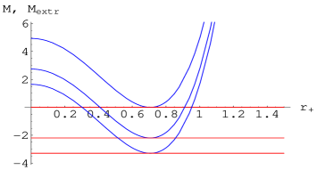
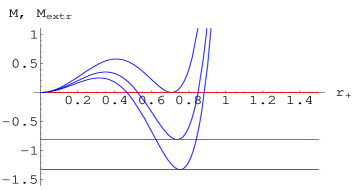
Figure 1: The ADM mass $M$ (curved lines) and extremal mass $M_{extr}$ (horizontal lines) as functions of the horizon. The values are fixed at $l=1$, $16\pi G=1$, and (upper plot) $n=4$, $V_{3}=2\pi^{2}$, $k=-1$, and $\alpha=1/4,~{}1/12,~{}0$ (top to bottom); (lower plot) $n=6$, $V_{3}=\pi^{3}$, $k=-1$, and $\alpha=1/4,\,17/100,\,0$ (top to bottom).

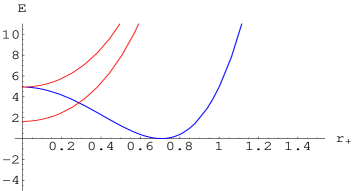
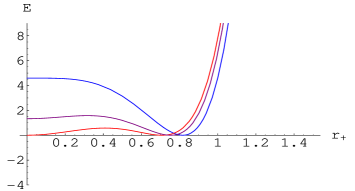
Figure 2: The energy $E$ as a function of horizon ($r_{+}$). The values are fixed at $l=1$, $16\pi G=1$, and $n=4$ (upper plot), $V_{3}=2\pi^{2}$, $k=+1$ (curves that grow with $r_{+}$) at $\alpha=1/4,1/12$ (upper to lower), and $k=-1$ (curve that has minimum at $r_{+}=r_{extr}$); $n=6$ (lower plot), $V_{3}=\pi^{3}$, $k=-1$, and $\alpha=1/4,17/100,0$ (top to bottom along the $E$-axis).

The total energy of hyperbolic black holes depends on the coupling $\alpha$ when $n>4$, and it has a local minimum at the extremal horizon position, which is seen also from the plots in Figs. 1 and 2. Even for the coupling $\alpha=l^{2}/4$, the total energy, for example, when $n=6$,

$$E=\frac{5V_{5}}{16\pi G_{7}}\left(-\,r_{+}^{4}+\frac{r_{+}^{6}}{l^{2}}+\frac{r_{+}^{2}l^{2}}{4}\right)$$ (24)

is vanishing at the extremal horizon $r_{+}=l/\sqrt{2}$. But, since $E$ is negative in the range $0<r_{+}<l/\sqrt{2}$, a massless extremal state can violate the positive energy theorem, but a negative mass extremal state with $\alpha<l^{2}/4$ always respects the energy condition $E\geqslant 0$.

III.2 Thermodynamic instability for $k=-1$

Here we adopt a Euclidean path integral formulation along with a consideration that the (extremal) entropy and specific heat are non-negative at the background. One also notes that the black hole entropy is always positive for the $k=\{0,1\}$ family. However, for $k=-1$, the inequality $r_{+}^{2}\geqslant 2\alpha$, which must hold in order to have a black hole interpretation, does not guarantee that the (extremal) entropy and specific heat are always positive, rather one must satisfy $r_{+}^{2}\geqslant 2(n-1)\alpha/(n-3)$. There is indeed an upper bound in the coupling constant $\alpha$ which ensures a thermodynamical stability; e.g., when $n+1=7$, the positivity of extremal entropy requires $r_{+}^{2}>10\,\alpha/3$ and hence $\alpha/l^{2}<17/100$. In particular, when one approaches the $\mu_{extr}=0$ limit at $4\alpha=l^{2}$, so $M_{extr}=0$, the specific heat could be negative, which mimics thermodynamic instability of the solution.

In the canonical ensemble, which should be the case here as we are considering uncharged black holes, the second derivative of the Euclidean action $\widehat{I}~{}(=\beta E-{\cal S})$ along the path parameterized by $x$ is

$$\left(\frac{\partial^{2}\hat{I}}{\partial^{2}\,x}\right)_{T}=\frac{1}{\beta^{2}}\,\left(\frac{d\beta}{dx}\right)^{2}\,\frac{dE}{dT}\,,$$ (25)

where $x=x(T)$ is the parameter that labels the path in the Euclidean path integral formulation. Thus, as discussed in Reall01a , the black hole is not the local minimum of the action when the specific heat $dE/dT$ is negative.

IV Specific heat and free energy curves and thermal phase transition

In Einstein gravity ($\alpha^{\prime}=0$), small spherical black holes have negative specific heat but large size black holes have positive specific heat Gregory93a . There exists a discontinuity of the specific heat as a function of temperature at $r_{+}=l/\sqrt{2}$, and so small and large black holes are somewhat disjoint objects. However, this is not essentially the case when $\alpha^{\prime}$ is nontrivial, and specially, in the spherical AdS₅ case, the small black holes also have positive specific heat IPN02a (see also the discussion in Ref. Cai01a ).

Here we study the AdS₅ and AdS₇ black holes, which are of some particular interest in string or M theory as they may provide duals for CFTs describing the world-volume theory for $N$ parallel $D3$- or $M5$-branes.

IV.1 Specific heat for hyperbolic black holes

In the AdS₅ case, the specific heat curve has a single branch for $\alpha=l^{2}/4$ and two branches for $\alpha<l^{2}/4$. The first cusp on the left, which will almost coincide with the $r_{+}$ axis for $\alpha\ll{l}^{2}$, has negative specific heat, so is unstable. Moreover, the entropy formula

$${\cal S}=\frac{V_{3,k=-1}\,r_{+}^{3}}{4G_{5}}\left(1-\frac{6\alpha}{r_{+}^{2}}\right)\,$$ (26)

shows that the extremal entropy is non-negative only if $\alpha\leqslant l^{2}/12$. It is then relevant to ask what would happen in the limit $l^{2}/4>\alpha>l^{2}/12$. As a specific example, for $\alpha=l^{2}/8$, the period $\beta=\pi l^{2}\left(4r_{+}^{2}-l^{2}\right)/[2r_{+}\left(2r_{+}^{2}-l^{2}\right)]$ is negative only in the range $0.5<r_{+}<0.707$. But when $\alpha=l^{2}/8$, the entropy in Eq. (26) becomes negative in the range $l^{2}/2<r_{+}^{2}<3l^{2}/4$, although $\beta$ is positive there. Thus, hyperbolic AdS₅ black holes are thermodynamically stable only if $\alpha\leqslant l^{2}/12$, i.e., when ${\cal S}_{extr}\geqslant 0$ (see Fig. 3).

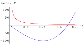
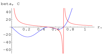
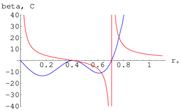
Figure 3: The Euclidean period $\beta$ (curves that asymptote to the $C$ or/and $r_{+}$ axes) and specific heat (curves with one or more cusps) vs horizon position $r_{+}$. The values are fixed at $l=1$, $n=4$, $V_{3}/16\pi G=2\pi^{2}$, $k=-1$, and $\alpha=1/4$, $\alpha=1/8$ and $\alpha=1/12$ (top to bottom plots).

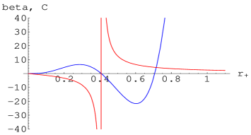
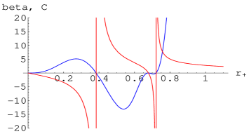
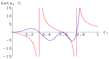
Figure 4: The Euclidean period (curves that asymptote to the $C$ or/and $r_{+}$ axes) and specific heat (curves with two or more cusps) vs horizon position $r_{+}$. The values are fixed at $l=1$, $n=6$, $V_{5}/16\pi G=\pi^{3}$, $k=-1$, and $\alpha=0.25$, $\alpha=0.23$, and $\alpha=17/100$ (top to bottom plots).

The free energy of a black hole is background dependent, while the Hawking temperature is not. But the formulas $C=dE/dT$ and $C=dM/dT$ give the same answer since $M_{extr}$ is $r_{+}$ or $T$ independent. In the AdS₅ case, the specific heat can be negative for a small $r_{+}$, specially, if $\alpha>l^{2}/12$. This particular feature is, although not totally new, different from the $k=+1$ case. For $k=+1$, a thermodynamic instability may arise due to a finite size effect, viz., a black hole of size $r_{+}\leqslant l/\sqrt{2}$ is unstable, $r_{+}>l$ is stable, and $l>r_{+}>l/\sqrt{2}$ is only locally preferred but globally unstable. However, for $k=-1$, instability may arise from the both a large coupling effect ($\alpha\sim l^{2}$) and a small size effect ($r_{+}<l$).

For the AdS₇ case, the extremal entropy is zero when $\alpha=17l^{2}/100$, for which the Euclidean period is

$$\beta=\frac{4\pi r_{+}l^{2}(50r_{+}^{2}-17l^{2})}{(10r_{+}^{2}-l^{2})(30r_{+}^{2}-17l^{2})}\,.$$ (27)

This is negative when $0<r_{+}<0.3162$ and $0.5831<r_{+}<0.7528$. The free energy is also negative in the latter range. That is, the first and third cusps in the bottom plot of Fig. 4 should be mirror reflected. There is no black hole interpretation for the first cusp. For $\alpha=l^{2}/4$, there are only two cusps, because in this case two unstable branches (the second and third cusps that appear for $\alpha<l^{2}/4$) merge to a single cusp, which has negative specific heat. We easily see that the thermodynamic stability of hyperbolic black holes in $n=6$ requires $\alpha/l^{2}\leqslant 17/100$. As a result, the specific heat and extremal entropy are positive at the background.

Moreover, for $k=-1$, the entropy of a black hole may appear to be negative, typically in the strong coupling limit $\alpha\sim l^{2}$; see, for example, Nojiri02a . But this parameter space must be excluded as an unphysical region because such a state is not stable classically nor do the supergravity approximations allow one to take $\alpha$ in the same order as $l^{2}$. As a result, for $\alpha\ll{l}^{2}$, the hyperbolic black hole is still stable and has positive entropy.

IV.2 Free energy for hyperbolic black holes

In Ref. Klemm99a , it was argued that the stringy corrections of order ${\alpha^{\prime}}^{3}{R}^{4}$ do not give to rise a thermal phase transition for flat and hyperbolic horizons, as a function of temperature. But using an AdS soliton as the thermal background of AdS black holes with Ricci flat horizons, a phase transition that is dependent not only on the Hawking temperature but also on the black hole area was found in Surya01a . This may imply that for the flat space $I\!\!R^{n-1}$ compactified down to a torus, and possibly also for the quotient of hyperbolic space $H^{n-1}/\Gamma$, the choice of ground state is crucial to see a possible phase transition. Here we want to use the obtained thermodynamic quantities to determine a thermal phase structure in the Einstein-Gauss-Bonnet gravity.

In the limit $0<r_{+}^{2}\leqslant 2(n-1)\alpha/(n-3)$, the behavior of extremal entropy is somewhat exotic, and so the second law of thermodynamics may not hold. In addition, for a hyperbolic AdS₅ black hole, the free energy scales with the coupling $\alpha$, but the energy (or energy density) does not (Fig. 5 and Eq. (23)). The total energy $E$ is vanishing at the extremal horizon, where $\beta=\infty$, but the free energy can be positive, zero, or negative there depending upon the coupling $\alpha$. As a result, the entropy is non zero at the extremal state, in particular, for a zero or small coupling $\alpha$. This result is consistent with the earlier observations made in Emparan99a ; Emparan99b with $\alpha^{\prime}=0$; a common thread in these results is that $\mbox{lim}_{\beta\to\infty}\beta F=$ finite. The meaning of a non zero extremal entropy may be traced back to the observation of “precursor” states first made in Susskind99a , when studying a short distance behavior of AdS$/$CFT duality.

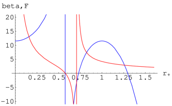
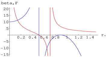
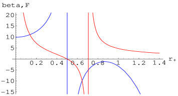
Figure 5: The Euclidean period (curves that asymptote to the $F$ or $r_{+}$ axis) and free energy (curves that are bounded from above or take finite values at $r_{+}=0$) vs horizon position $r_{+}$. The values are fixed at $k=-1$, $n=4$, $l=1$, $16\pi G=1$, $V_{3}=2\pi^{2}$, and, $\alpha=1/6,\,0.1305,\,1/8$ (top to bottom plots).

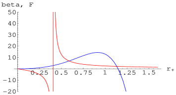
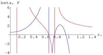
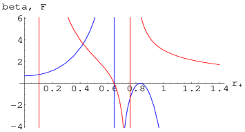
Figure 6: The Euclidean period (curves that asymptote to the $F$ or/and $r_{+}$ axis) and free energy (curves that have finite values at $r_{+}=0$ or bounded from above) vs horizon. The values are fixed at $k=-1$, $n=6$, $l=1$, $16\pi G=1$, $V_{5}=\pi^{3}$, and $\alpha=0.25,0.2162,0.2072$ (top to bottom plots).

The first plot in Fig. 6 corresponds to the $\mu_{extr}=0$ state with $\alpha=l^{2}/4$. In the lower two plots, the extremal state is shown by an asymptotic on the right, and the critical state, which is absent in AdS₅ (cf. Fig. 5), is shown by another asymptotic on the left. The middle vertical line, where the free energy diverges and $\beta=0$, corresponds to the horizon at $r_{+}^{2}=2\alpha$. For $\alpha<l^{2}/4$, the singularity at $r_{+}=\sqrt{2\alpha}$, where $\beta=0$, is hidden inside the extremal horizon, so is harmless.

When $n=4$ and $0.25\,l^{2}>\alpha>0.1305\,l^{2}$, the free energy appears to be positive in a certain range $r_{2}>r_{+}>r_{extr}$, where the Hawking-Page temperature is finite, but, for a small coupling $\alpha\ll{l}^{2}$, the free energy takes only the negative value for positive $\beta$. It takes a maximum value at the extremal state if ${\cal S}_{extr}=0$ (for example, at $\alpha=l^{2}/12$ when $n=4$). There is no thermal AdS phase for the coupling $\alpha<0.1305\,l^{2}$, and hence no phase transition appears to occur in this case.

IV.3 Free energy for spherical black holes

The spherical Gauss-Bonnet black holes were studied in Cai01a ; IPN02a in some detail, so we will be brief here. For this case, since $E=M$, the free energy is vanishing when

$$\alpha=\tilde{\alpha}=r_{+}^{2}\left[\frac{4\sqrt{n(n-3)}-(n-3)}{6(n-1)}\right].$$ (28)

This separates two other $F=0$ trajectories Cai01a :

$$\alpha_{\pm} = \pm\frac{r_{+}^{2}}{2}\sqrt{\frac{9\,r_{+}^{4}}{l^{4}}+\frac{(15-n)\,r_{+}^{2}}{(n-1)\,l^{2}}-\frac{(n+1)(7n-25)}{4(n-1)^{2}}}$$ (29)

$$+\,r_{+}^{2}\left(\frac{3\,r_{+}^{2}}{2\,l^{2}}-\frac{(n-7)}{4(n-1)}\right)\,.$$

Obviously, $n\geqslant 4$ is needed to ensure that $\alpha>0$. For example, when $n=4$, we find $r_{+}^{2}=18\alpha/7>2\alpha$. The $\alpha_{-}$ branch of the solutions gives a stable AdS solution when $\alpha\ll{l}^{2}$, while the $\alpha_{+}$ branch may be unstable.

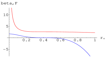
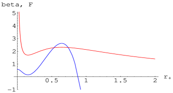
Figure 7: Inverse temperature $\beta$ (curves that asymptote to the $F$ and $r_{+}$ axes) and free energy (curves that cross $r_{+}$ axis) vs horizon position $r_{+}$ for spherical black holes. The values are fixed at $k=+1$, $n=4$, $l=1$, and, from top to bottom, $\alpha=0.0278$, $0.01$. A new branch of a stable black hole appears in the AdS₅ case.

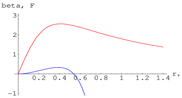
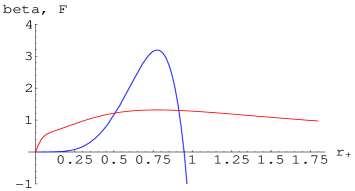
Figure 8: Inverse temperature $\beta$ (curves that asymptote to the $r_{+}$ axis) and free energy (curves that cross the $r_{+}$-axis) vs horizon position $r_{+}$ for spherical black holes. The values are fixed at $k=+1$, $n=6$, $l=1$, and, from top to bottom, $\alpha=0.1$, $\alpha=0.01$.

As in the $\alpha=0$ case, a spherical Gauss-Bonnet black hole presents an interesting thermal feature, namely, the Hawking-Page phase transition at finite temperature. In the AdS₅ case, as $\alpha$ is decreased, the free energy lowers toward zero at low temperature. For $\alpha\ll{l}^{2}$, in the small $r_{+}$ region, $F$ nearly approaches zero but it never touches the $F=0$ axis, e.g., when $\alpha/l^{2}=3\times 10^{-7}$, $F\sim 4\times 10^{-6}$. That is, the free energy curve crosses the $F=0$ axis only once, namely, when $r_{+}\lesssim l$, which corresponds to the Hawking-Page phase transition point.

For $\alpha/l^{2}\gtrsim 0.0278$, the free energy is a monotonically decreasing function of $r_{+}$ and the second branch (peak) on the right disappears. Using the relation ${\alpha^{\prime}}/l^{2}=1/\sqrt{2g^{2}N}$, we see that the Hawking-Page transition disappears at sufficiently small ’t Hooft coupling $g^{2}N$.

As for the charged AdS black holes Chamblin99a , the inverse temperature and free energy curves in Fig. 7 remind us of the behavior of a van der Waals gas in the Clapeyron $(V,P)$ phase, where the point of inflection in $\beta(r)$ signals a critical point. This behavior may be seen for spherical AdS black holes that receive stringy corrections of the form ${\alpha^{\prime}}^{3}R^{4}$ Klemm99a or $R_{abcd}R^{abcd}$ IPN02c .

One also notes that, in all dimensions $n>4$, the behavior of a Hawking-Page transition is qualitatively similar for small and large couplings, except that the free energy becomes more positive as $\alpha$ is decreased. But still, as in the AdS₅ case, a low temperature phase corresponds to a thermal AdS space with $F\geqslant 0$ and a high temperature phase corresponds to an AdS black hole with $F<0$.

V Stability analysis: metric perturbations

The stability of background metrics under gravitational perturbations can normally be checked from an analysis of whether bound states with a negative eigenstate exist. If the corresponding Schrödinger equations allow a state with $E<0$ and/or there are growing (quasi) normal modes at the event horizon, and/or the potential is negative and unbounded from below, then the spacetime metrics can be unstable.

V.1 Linearized field equations

Consider a linear perturbation of the metric

$$\bar{g}_{ab}\to g_{ab}=\bar{g}_{ab}+h_{ab}\,,\quad g^{ab}=\bar{g}^{ab}-h^{ab}$$

with $|h^{a}\,_{b}|\ll{1}\,.$ For $\alpha^{\prime}=0$, the linearized equations are

$$\delta R_{ab}=-\,nc\,h_{ab}\,,$$ (30)

where $c$ has the dimension of $\ell^{2}$. For $\alpha^{\prime}>0$ and $k=+1$, as evaluated in the Appendix, the perturbations $\delta g_{ab}~{}(=h_{ab})$ must satisfy

$$\left(1-2C\alpha\right)\delta R_{ab}=-\,n\,C\,\left(1-\frac{(3n^{2}-3n+2)C\alpha}{n(n-3)}\right)h_{ab}$$

$$~{}~{}~{}~{}~{}~{}~{}-\,\frac{2C\alpha}{n-3}\,\bar{g}_{ab}\left[\bar{\nabla}^{c}\bar{\nabla}^{d}h_{cd}-\bar{\nabla}^{2}h+C(n+1)h\right].$$

(31)

with

$$C=\frac{1}{2\alpha}\left(1\mp\sqrt{1+\frac{8\alpha\Lambda}{n(n-1)}}\,\right)\equiv\frac{1}{2\alpha}\left(1\mp\sqrt{1-\frac{4\alpha}{l^{2}}}\,\right).$$ (32)

For transverse trace-free (de Donder) perturbations, $h_{c}^{c}=\bar{\nabla}^{a}h_{ab}=0$, we obtain

$$2\delta R_{ab} = \left(\Delta_{L}h\right)_{ab}$$ (33)

$$= -\,\frac{2nC}{1-2C\alpha}\left[1-\frac{C\alpha(3n^{2}-3n+2)}{n(n-3)}\right]h_{ab}\,.$$

If the base ${\cal M}$ is hyperbolic, then it is not a priori sufficient to prove stability for the tensor modes only. In this case, the scalar and vector modes can also be unstable but we will not consider such modes here.

We wish to study the stability of the background metrics under the conditions

$$h_{0a}=h_{1a}=0\,.$$ (34)

With these constraints, along with a requirement that the base ${\cal M}$ is itself an Einstein space $\widetilde{R}_{ij}(h)=(n-2)k\,\tilde{g}_{ij}$, the transverse trace-free property of $h_{ab}$ is characterized by $h_{ij}$, where $i,\,j,\cdots$ run from $2$ to $n~{}(\equiv D-1)$,

$$2\delta R_{ij}=\left(\Delta_{L}h\right)_{ij}=-\,2nA\,h_{ij}\,,$$ (35)

with

$$\left(\Delta_{L}h\right)_{ij} = \frac{1}{r^{2}}\,\tilde{\Delta}_{L}h_{ij}-f\left(\frac{d^{2}}{dr^{2}}+\frac{4}{r^{2}}\right)h_{ij}$$

$$-\frac{rf^{\prime}+(n-5)f}{r}\,\frac{d}{dr}\,h_{ij}+\frac{1}{f}\,\frac{d^{2}}{dt^{2}}\,h_{ij}\,,$$

$$A = \frac{C}{1-2C\alpha}\,\left[1-\frac{C\alpha(3n^{2}-3n+2)}{n(n-3)}\right],$$ (36)

where $\tilde{\Delta}_{L}h_{ij}$ is the Lichnerowicz operator acting on ${\cal M}$. We look for unstable tensor modes of the form

$$h_{ij}(x)=r^{2}\,\phi(r)\,e^{\omega t}\,\widetilde{h}_{ij}(\tilde{x}),$$ (37)

where $(\tilde{x})$ are coordinates on ${\cal M}$. It is convenient to assume that

$$\left(\widetilde{\Delta}_{L}\widetilde{h}\right)_{ij}=\lambda\,\widetilde{h}_{ij},$$ (38)

where $\lambda$ is the eigenvalue of the Lichnerowicz operator. Equation (35) then takes the form of a Sturm-Liouville type problem Gibbons02a

$$-\,f\frac{d}{dr}\left(f\,r^{n-1}\,\frac{d\phi(r)}{dr}\right)$$

$$~{}~{}-\,\frac{2f}{r^{2}}\,\left((n-2)f-\frac{\lambda}{2}+r\,f^{\prime}-nA\,r^{2}\right)\phi(r)$$

$$~{}~{}=\omega^{2}\,\phi(r)\,r^{n-1}\,.$$ (39)

In terms of Regge-Wheeler type coordinates $dr\equiv f\,dr_{*}$ and $\phi(r)\equiv\Phi\,r^{-(n-1)/2}$, this takes the form

$$\frac{d^{2}\Phi}{dr_{*}^{2}}-V\left(r(r_{*})\right)\Phi=\omega^{2}\Phi,$$ (40)

where

$$V(r) = \frac{\lambda\,f}{r^{2}}+\frac{\left[(n-2)(n-10)-1\right]f^{2}}{4r^{2}}+\frac{(n-5)ff^{\prime}}{2r}$$ (41)

$$~{}~{}~{}~{}~{}~{}~{}~{}~{}~{}~{}~{}~{}~{}~{}~{}~{}~{}~{}~{}~{}~{}~{}~{}~{}~{}~{}~{}~{}~{}~{}~{}~{}~{}+2nA\,f.$$

A requirement of finite energy is equivalent to the normalization condition that $\int\Phi^{2}\,dr_{*}=\int f(r)^{-1}\,\Phi^{2}\,dr$ is finite. Usually, the stability of a potential depends on the eigenvalues of the Lichnerowicz operator, ensuring that the potential is positive and bounded from below.

V.2 Stability of massless state in general relativity

The Schwarzschild black hole is stable in four dimensions Vishves70a . It is also learnt that a spherically symmetric AdS₄ black hole is stable against small electromagnetic and gravitational perturbations Cardoso01a . The issue of instability of tensor modes, however, arises only for $n+1>4$ since there are no tensor harmonics on $S^{2}$ or $H^{2}$.

For a vanishing cosmological constant ($\Lambda=0$), so that $A=0$, the spacetime metric is flat if the base is a sphere, and if the base is not a sphere then the full spacetime is a cone which is singular at the origin. Thus, for $\Lambda=0$, we must take $k=1$, so that $f(r)\to 1$ asymptotically and $r=r_{*}$. Then the asymptotic potential is

$$V_{\infty}(r)=\frac{4\lambda+(n-2)(n-10)-1}{4\,r^{2}}=\frac{(2\nu-1)(2\nu+1)}{4\,r^{2}}\,.$$ (42)

This potential is non-negative only if

$$\lambda \geqslant \frac{1+(n-2)(10-n)}{4}\,,$$

$$or\quad\nu = \frac{1}{2}\,\sqrt{(n-2)(n-10)+4\lambda}\geqslant\frac{1}{2},$$ (43)

where $V_{\infty}(r)=0$ if equality holds. Stability of a potential requires that there are no bound negative energy states or no growing modes with $\omega>0$ at the horizon, if the latter exists. A requirement that $\lambda>0$ indeed constraints the spacetime dimensions $D=(n+1)$ to $n\leqslant 10$. The asymptotic solution for $\Phi(r)$ that decays as $r$ goes to $+\infty$ is

$$\Phi_{\infty} = C_{1}\,\sqrt{r}\,J_{\nu}\left(\sqrt{-\omega^{2}}\,r\right)+C_{2}\,\sqrt{r}\,~{}Y_{\nu}\left(\sqrt{-\omega^{2}}\,r\right)$$ (44)

$$= \mbox{Re}\left[\sqrt{r}\,K_{\nu}(\omega r)\right].$$

For small $r$ and a real positive $\nu$, $\Phi_{\infty}(r)$ behaves as $\sim r^{-\nu+1/2}$. This solution is divergent but normalizable if $1>\nu>1/2$, and divergent and non-normalizable if $\nu\geqslant 1$. For $n\leqslant 10$, an imaginary $\nu$ does not exist with a positive potential, while, for $n>10$, the eigenvalue $\lambda$ may take a negative value, so $\nu>1$, but this solution is always non-normalizable.

For $\Lambda<0$, the potential (42) is modified to

$$V(r) = \left(\frac{4\lambda+(n-2)(n-10)-1}{4\,r^{2}}+\frac{(n-1)(n+1)}{4\,l^{2}}\right)$$

$$~{}~{}~{}~{}~{}~{}~{}~{}~{}~{}~{}~{}~{}~{}~{}~{}~{}~{}~{}~{}~{}~{}\times\left(1+\frac{r^{2}}{l^{2}}\right)$$

$$V(x) = \frac{1}{l^{2}}\Bigg{(}\frac{4(\lambda-n+1)+(n-3)(n-5)}{4\,x}$$ (45)

$$~{}~{}~{}~{}~{}~{}~{}~{}~{}~{}~{}~{}~{}~{}+\,\frac{(n-1)(n+1)}{4}\Bigg{)}\left(1+x\right),$$

where $x\equiv r^{2}/l^{2}$. This is always positive and bounded from below in satisfying Eq. (V.2). The Schrödinger equation may be expressed as a hypergeometric equation

$$x(x+1)^{2}\,\Phi^{\prime\prime}(x)+\frac{(x+1)(3x+1)}{2}\,\Phi^{\prime}(x)$$

$$~{}~{}-\,\frac{x+1}{4}\times\Bigg{(}\frac{4\lambda+(n-2)(n-10)-1}{4x}$$

$$~{}~{}~{}~{}~{}+\,\frac{(n-1)(n+1)}{4}+\frac{\omega^{2}\,l^{2}}{(x+1)}\Bigg{)}\Phi(x)=0,$$ (46)

with no singularities in the range $0<x<\infty$. To simplify (V.2) one can make the following substitutions:

$$2\nu = \sqrt{4\lambda+(n-2)(n-10)},\quad\sigma=-\,\frac{i\omega\,l}{2},$$

$$a = \sigma+\frac{2\nu-(n-2)}{4}\,,\quad b=\sigma+\frac{2\nu+(n+2)}{4}\,,$$ (47)

$$~{}~{}~{}~{}~{}~{}~{}~{}~{}~{}~{}~{}~{}~{}~{}~{}~{}c=\nu+1\,.$$

Under the decomposition $\Phi(x)=x^{(1+2\nu)/4}\,(1+x)^{\sigma}\,\varphi(x)$, two independent solutions of Eq. (V.2) are found to be

$$\varphi(x)=\left\{\begin{array}[]{l}{}_{2}F_{1}(a,\,b;\,c;\,-\,x),\\ x^{1-c}\,~{}{}_{2}F_{1}(a-c+1,\,b-c+1;\,2-c;\,-\,x),\end{array}\right.\$$ (48)

where ${}_{2}F_{1}(a,b;c;x)$ is the hypergeometric function, and the parameter $c\neq 0,-1,-2,-3,\cdots$ for the first solution, and $c\neq 2,3,4,\cdots$ for the second solution. A general solution of Eq. (V.2) is given by a linear combination of

$$\Phi_{\pm}(x) = x^{(1\pm 2\nu)/4}\,\left(1+x\right)^{-\,i\omega l/2}{}_{2}F_{1}\Bigg{(}\frac{\pm\,2\nu-(n-2)}{4}$$

$$-\frac{i\omega l}{2},\,\frac{\pm\,2\nu+(n+2)}{4}-\frac{i\omega l}{2};\,\pm\,\nu+1;\,-\,x\Bigg{)}.$$

A stability check may be needed in both limits $x\to 0$ and $x\to\infty$. This is the case studied by Gibbons and Hartnoll Gibbons02a in some detail. For consideration of the $\alpha>0$ case in the next section, we briefly discuss first some important features of the solution with $\alpha^{\prime}=0$.

To study the asymptotic behavior, one uses the following relation of the hypergeometric functions Askey

$${}_{2}F_{1}(a,b;c;x) = h_{1}(-x)^{-a}{}_{2}F_{1}\left(a,a-c+1;a-b+1;\frac{1}{x}\right)$$

$$+ h_{2}\,(-x)^{-b}\,{}_{2}F_{1}\left(b,\,b-c+1;b-a+1;\frac{1}{x}\right),$$

where

$$h_{1}=\frac{\Gamma(c)\Gamma(b-a)}{\Gamma(c-a)\Gamma(b)}\,,\quad h_{2}=\frac{\Gamma(c)\Gamma(a-b)}{\Gamma(c-b)\Gamma(a)}\,.$$ (51)

As $x\to\infty$, the asymptotic solution is given by

$${}_{2}F_{1}(a,b;c;x)=h_{1}(-x)^{-a}\left(1+\frac{a(a-c+1)}{a-b+1}\frac{1}{x}+\cdots\right)$$

$$~{}~{}~{}~{}~{}~{}~{}~{}~{}+\,h_{2}(-x)^{-b}\left(1+\frac{b(b-c+1)}{b-a+1}\frac{1}{x}+\cdots\right).$$ (52)

The boundedness requires that as $r\to\infty$ the function $\Phi(r)$ must go as ${\cal O}\left(r^{(n-1)/2}\right)$ or a lower power of $r$. A solution that has this behavior is given by a linear combination of $\Phi_{\pm}$ such that the term $(x)^{-b}$ of the two solutions cancels. Hence,

$$\Phi_{3}(x) = x^{-(n+1)/4+i\omega\,l/2}\,\left(1+x\right)^{-\,i\omega\,l/2}$$ (53)

$$\times {}_{2}F_{1}\Bigg{(}\frac{2\nu+n+2}{4}-\frac{i\omega\,l}{2},\,\frac{-\,2\nu+n+2}{4}-\frac{i\omega\,l}{2};$$

$$~{}~{}~{}~{}~{}~{}~{}~{}~{}~{}~{}~{}~{}~{}~{}~{}~{}\,\frac{n+2}{2};\,-\,\frac{1}{x}\Bigg{)}\,.$$

To evaluate the behavior as $r\to 0$, one can apply Eq. (LABEL:infinite) to Eq. (53), replacing $1/x$ by $x$ for ${}_{2}F_{1}$. The leading behavior of the solution as $x\to 0$ is given by ${\cal O}\left(x^{-(n+1+2\nu-n-2)/4}\right)\sim{\cal O}\left(r^{(1-2\nu)/2}\right)$. The range of convergence for $c>a+b$ is $|x|<1$ and $x=1$, which implies that $0>-\,i\omega\,l$. That is, a situation that the hypergeometric series terminates for some special (positive) values of $\omega$ simply does not arise in the above case. As a result, the massless configurations where ${\cal M}$ has constant positive ($k=+1$) curvature are stable under tensor perturbations.

V.3 Instability of massless topological black holes

A dynamical instability of topological black holes in Einstein gravity, under tensor perturbations, was studied in Ref. Gibbons02a . So we will be brief in our analysis of this particular case, but we shall review some results reported earlier as a quantitative difference arises. For $\alpha=0$, and $k=-1$, $\mu=0$, the metric solution is

$$f(r)=-1+\frac{r^{2}}{l^{2}}\,.$$ (54)

The gravitational potential then takes the form

$$V(x) = \frac{1}{l^{2}}\Bigg{(}\frac{4(n-1+\lambda)-(n-3)(n-5)}{4\,x}$$ (55)

$$~{}~{}~{}~{}~{}~{}+\,\frac{(n-1)(n+1)}{4}\Bigg{)}\left(x-1\right),$$

where $x\equiv r^{2}/l^{2}$. One may easily check that this potential is positive for all values of $x$ only if

$$\lambda=5-3n\equiv\tilde{\lambda}\,.$$ (56)

This is a special situation. Since the Lichnerowicz spectrum is bounded below by $\lambda_{min}=-\,2(n-1)$, the spacetime dimension $n+1=4$ is on the borderline for which $\tilde{\lambda}=\lambda_{min}$. For $n+1\geqslant 5$, $\tilde{\lambda}$ is smaller than $\lambda_{min}$, and the potential can be negative and unbounded. More precisely, as the plots in Fig. 9 show, the potential is negative but bounded from below when

$$\lambda<\lambda_{crit}=\frac{(n-2)(n-10)-1}{4}\,,$$ (57)

and unbounded when $\lambda\geqslant\lambda_{crit}$; the latter might signal instability of a massless topological black hole.

To gather more information, we need to solve the full differential equation. The Schrödinger equation, under the potential (55), may be expressed as

$$x(x-1)\,\Phi^{\prime\prime}(x)+\frac{x+1}{2}\,\Phi^{\prime}(x)-\frac{1}{4}\,\Bigg{(}\frac{(n-1)(n+1)}{4}$$

$$+\frac{4\lambda+1-(n-2)(n-10)}{4x}+\frac{\omega^{2}\,l^{2}}{4}\,\frac{1}{x-1}\Bigg{)}\Phi(x)=0\,.$$

(58)

Let us make the following substitutions:

$$2\tilde{\nu} = \sqrt{4(2-\lambda)+(n-2)(n-10)}\,,\quad\tilde{\sigma}=-\,\frac{\omega\,l}{2},$$

$$a = \tilde{\sigma}+\frac{2\tilde{\nu}+(n+2)}{4}\,,\quad b=\tilde{\sigma}+\frac{2\tilde{\nu}-(n-2)}{4}\,,$$ (59)

$$~{}~{}~{}~{}~{}~{}~{}~{}~{}~{}~{}~{}~{}~{}~{}~{}~{}c=\tilde{\nu}+1,$$

and decompose the harmonic function as $\Phi(x)=x^{(3+2\tilde{\nu})/4}\,{(x-1)}^{\tilde{\sigma}}\,\varphi(x)$. Then two independent solutions of Eq. (V.3) are easily written as

$$\varphi(x)=\left\{\begin{array}[]{l}{}_{2}F_{1}(a,b;c;x),\\ x^{1-c}{}_{2}F_{1}(a-c+1,b-c+1;2-c;x).\end{array}\right.\$$ (60)

The general solution of Eq. (V.3) is given by a linear combination of the following two solutions:

$$\Phi_{\pm}(x)=x^{(3\pm 2\tilde{\nu})/4}\,\left(x-1\right)^{-\,\omega\,l/2}\times$$

$${}_{2}F_{1}\Bigg{(}\frac{\pm\,2\tilde{\nu}+(n+2)}{4}-\frac{\omega\,l}{2},\,\frac{\pm\,2\tilde{\nu}-(n-2)}{4}-\frac{\omega\,l}{2};$$

$$~{}~{}~{}~{}~{}~{}~{}~{}~{}~{}~{}~{}~{}~{}~{}~{}~{}~{}~{}~{}~{}~{}~{}~{}\,\pm\,\tilde{\nu}+1;\,\,x\Bigg{)}.$$ (61)

The boundedness requires that as $r\to\infty$ the function $\Phi(r)$ must go as ${\cal O}\left(r^{(n-1)/2}\right)$ or a lower power of $r$. The solution that has this behavior is given by a linear combination of $\Phi_{\pm}$ such that the term $(-x)^{-b}$ of two solutions cancel, and hence the asymptotic behavior goes like ${\cal O}\left(x^{(3\pm 2\tilde{\nu}\mp 2\tilde{\nu}-n-2)/4}\right)\sim{\cal O}\left(r^{-(n-1)/2}\right)$. The solution that is well behaved as $r\to\infty$ reads

$$\Phi_{3}(x) = x^{(2\omega l-n+1)/4}\left(x-1\right)^{-\,\omega{l}/2}{}_{2}F_{1}\Bigg{(}\frac{2\tilde{\nu}+n+2}{4}-\frac{\omega{l}}{2},$$ (62)

$$\frac{-2\tilde{\nu}+n+2}{4}-\frac{\omega\,l}{2};\frac{n+2}{2};\frac{1}{x}\Bigg{)}.$$

We can find a new solution of the hypergeometric equation by using the relation

$${}_{2}F_{1}\left(a,\,b;\,c;\,x\right) = k_{1}~{}{}_{2}F_{1}\left(a,\,b;\,a+b+1-c;\,1-x\right)$$ (63)

$$+\,k_{2}\left(1-x\right)^{c-a-b}{}_{2}F_{1}\Big{(}c-b,c-a;$$

$$1+c-a-b;1-x\Big{)},$$

where

$$k_{1}=\frac{\Gamma(c)\Gamma(c-a-b)}{\Gamma(c-a)\Gamma(c-b)}\,,\quad k_{2}=\frac{\Gamma(c)\Gamma(-c+a+b)}{\Gamma(a)\Gamma(b)}\,.$$ (64)

For a generic solution with $k_{1},k_{2}\neq 0$, the dominant term as $x\to 1$ is ${\cal O}\left((x-1)^{-\omega{l}/2}\right)$. This solution is not square integrable at $x=1$. In the special case, with $k_{1}=0$, which is accomplished by choosing $c=a$ or $c=b$, one finds a solution with better behavior at $x=1$. In this case, the leading term as $x\to 1$ is

$$(x-1)^{-\omega\,l/2}\,\left(\frac{x-1}{x}\right)^{\omega\,l}={\cal O}\left((x-1)^{\omega\,l/2}\right).$$ (65)

This solution is normalizable and bounded at the horizon for $\omega>0$. However, the condition that either $(c-a)$ or $(c-b)$ is zero would be that

$$\omega=\left(\frac{2\tilde{\nu}-(n+2)}{2\,l}\right)>0\,.$$ (66)

This holds if $2\tilde{\nu}>n+2$ or equivalently, $\lambda_{min}<(6-4n)$ [cf., Eq. (V.3)], which is not allowed since the Lichnerowicz spectrum is bounded below by $\lambda_{min}=-\,2(n-1)$. In the following range of the eigenvalues, which are allowed in the theory such that $2\tilde{\nu}>1$:

$$\frac{(n-2)(n-10)-1}{4}\leqslant\lambda<\frac{(n-2)(n-10)+8}{4},$$ (67)

we still have $\lambda>\lambda_{min}$, the gravitational potential is always unbounded from below. In Gibbons02a a massless $k=-1$ background was expected to be classically gravitationally stable if the $\lambda>\lambda_{crit}$. Whether this interpretation is correct is not clear a priori since one would not expect to have a classically stable background if the potential is negative and unbounded from below.

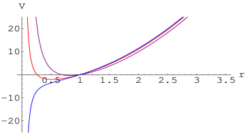
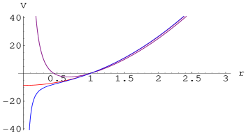
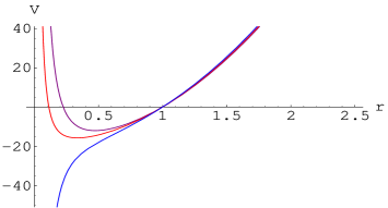
Figure 9: The potential as a function of the horizon $r_{+}$ at fixed $l=1$: (top panel) $n=4$ and $\lambda=-\,5,-\,14/4,-\,3$ (top to bottom); (middle panel) $n=6$ and $\lambda=-\,6,-\,17/4,-\,4$ (top to bottom); (bottom panel) $n=9$ and $\lambda=-\,3,~{}-\,9/4,~{}-\,1$ (top to bottom). The above potential will be bounded and positive only for $\lambda=5-3n$, and it is always unbounded for $\lambda$ satisfying Eq. (67).

In Aros02a , by taking the massless $k=-1$ black hole itself as a ground state, an analytic result for the quasinormal modes of a scalar perturbation was presented for $n\geqslant 3$. Here we emphasize that a metric background with $k=-1$ and $\mu=0$ may be unstable under tensor perturbations. Let us give some specific examples. Instability of the $\mu=0$, $k=-1$ spacetime may arise when

$$n=4:\quad-\,\frac{13}{4}\leqslant\lambda<-\,1,$$

$$n=6:\quad-\,\frac{17}{4}\leqslant\lambda<-\,2,$$

$$n=9:\quad-\,2\leqslant\lambda<\frac{1}{4}.$$

In these ranges, the gravitational potential is negative and unbounded from below. Although a negative potential does not necessarily imply instability of a background, an unbounded potential certainly signals instability of the background metric with $\mu=0$ and $k=-1$.

V.4 Stability of negative mass extremal state

When $\alpha^{\prime}=0$, the extremal solution is given by

$$f(r)=-1+\frac{r^{2}}{l^{2}}+B\left(\frac{l}{r}\right)^{n-2}\,,\quad B=2\sqrt{\frac{(n-2)^{n-2}}{n^{n}}}\,.$$ (68)

The gravitational potential therefore reads

$$V(r) = \Bigg{[}\frac{4(n-1+\lambda)-(n-3)(n-5)}{4{r}^{2}}+\frac{(n-1)(n+1)}{4{l}^{2}}$$ (69)

$$-\,\frac{B(n-1)^{2}l^{n-2}}{4r^{n}}\Bigg{]}\left[-1+\frac{r^{2}}{l^{2}}+B\left(\frac{l}{r}\right)^{n-2}\right].$$

The spacetime one is allowed to take is $r>r_{extr}=l\,\sqrt{(n-2)/n}$.

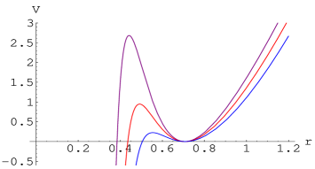
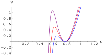
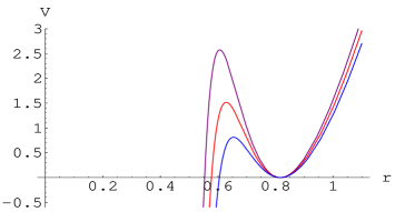
Figure 10: The potential defined for a negative mass extremal background with $\alpha=0$. The values are chosen, from top to bottom, at (top panel) $n=4$ and $\lambda=0,-1$, and $-2$; (middle panel) $n=5$ and $\lambda=-1,-2$, and $-3$; (bottom panel) $n=6$ and $\lambda=-2,-3$, and $-4$.

For $n=4$, the metric function (68) takes the form

$$f(x)=\frac{(2x-1)^{2}}{4x}\,,$$ (70)

where $x\equiv r^{2}/l^{2}$ is a dimensionless scale. As there is no cosmological horizon for an extremal solution, the perturbation extends to $x\to\infty$. The potential

$$V(x)=\frac{1}{l^{2}}\,\left(\frac{4(3+\lambda)+1}{4\,x}+\frac{15}{4}-\frac{9}{16\,x^{2}}\right)\left(\frac{(2x-1)^{2}}{4\,x}\right)\,$$ (71)

vanishes at the extremal horizon $2x=1$, but it is everywhere positive outside the extremal horizon. Under this potential, the Schrödinger equation takes the form

$$\frac{(2x-1)^{2}}{8x^{2}}\Bigg{[}2x(2x-1)^{2}\,\Phi^{\prime\prime}(x)+(4x^{2}-1)\,\Phi^{\prime}(x)$$

$$~{}-\,2x\left(\frac{4(3+\lambda)+1}{4{x}}+\frac{15}{4}-\frac{9}{16x^{2}}\right)\Phi(x)\Bigg{]}$$

$$~{}~{}~{}~{}~{}~{}-\omega^{2}l^{2}\,\Phi(x)=0.$$ (72)

The condition of boundedness is automatic, because it simply requires that $\Phi(x)$ is bounded at $2x=1$, where $f(x)=0$. The finite energy condition will be that $\Phi(x)$ goes to zero on the extremal horizon, because the zero of $f(x)$ is simple. We can get some insights into the stability of the solutions also by inspecting the plots for the gravitational potential.

The hypergeometric equation (V.4) can be solved exactly only for the $\omega=0$ modes:

$$\Phi(x) = c_{1}\,(2x-1)^{-\,\gamma/4}\,x^{3/4}{}_{2}F_{1}(a,b;1;2x)$$ (73)

$$+\,c_{2}\,(2x-1)^{-\,\gamma/4}\,x^{3/4}{}_{2}F_{1}(a,b;1,2x)$$

$$\,\times\int\frac{(2x-1)^{-1+\gamma/2}}{x\,\left[{}_{2}F_{1}(a,b;1;2x)\right]^{2}}\,dx,$$

where

$$\gamma=\sqrt{2\lambda+32}\,,\quad a=\frac{6-\gamma}{4}\,,\quad b=\frac{-\,(2+\gamma)}{4}\,.$$ (74)

This solution converges at $2x=1$ for any eigenvalue $\lambda>\lambda_{crit}$, and also in the range (67), and it is also normalizable there. The situation is similar in the $n>4$ case. Now for the eigenvalues $\lambda$ in the range given by Eq. (67), where one might expect instability to arise for a massless background, the potential is bounded and positive. Therefore, in the spacetime region $r\geqslant r_{extr}$, the potential is always positive, tending to zero at the extremal state. This means that the extremal ground state may be stable under tensor perturbation.

For $n=6$, the metric function (68) takes the form

$$f(x)=\frac{(3x+1)(3x-2)^{2}}{27\,x^{2}}\,,$$ (75)

and the corresponding potential is

$$V(x) = \frac{1}{l^{2}}\,\left(\frac{4\lambda+17}{4x}+\frac{35}{4}-\frac{25}{27\,x^{2}}\right)$$ (76)

$$~{}~{}~{}~{}~{}~{}\times\left(\frac{(3x+1)(3x-2)^{2}}{27\,x^{2}}\right)\,.$$

This does not cover the small $x$ region; for example, when $\lambda=-13/4$, the potential is not bounded from below when $x<0.27$. That is, the spacetime region $r<r_{e}$ may have an internal infinity, where the potential is not well behaved, and the reference spacetime is incomplete in Einstein gravity, especially for the $k=-1$ case. This is clearly seen from the plots of gravitational potential $V(r)$ vs horizon position in Fig. 10. This problem may be resolved once the background metric and hence the potential receives higher derivative curvature corrections.

VI Gauss-Bonnet black holes and Gravitational Stability

In this section, we study the stability of metric backgrounds with a non trivial GB coupling. With $\mu=0$, the AdS vacuum solution is given by

$$f(r)=k+\frac{r^{2}}{2\alpha}\left(1\mp\sqrt{1-\frac{4\alpha}{l^{2}}}\,\right)\equiv k+C\,r^{2}\,.$$ (77)

In this case, for any $k$, the spacetime metric has constant curvature. However, for $k=-1$, we take the negative mass extremal state as a ground state, which reads in five spacetime dimensions as

$$f(r)=-1+\frac{r^{2}}{2\alpha}\left[1-\sqrt{\left(1-\frac{4\alpha}{l^{2}}\right)\left(1-\frac{\alpha l^{2}}{r^{4}}\right)}\right]\,.$$ (78)

The metric spacetime is only asymptotically locally AdS, which can be easily seen by allowing a particular coupling. The requirement that $4\alpha<l^{2}$ is complementary to the condition $r^{2}\geqslant l^{2}/2$.

VI.1 Stability of a massless Gauss-Bonnet black hole

As shown in the previous section, for $\alpha=0$, the AdS black holes with $\mu=0$ and $k=+1$ are stable under tensor perturbations. Here we extend this analysis for a non trivial GB coupling. The background metric function, with $\alpha>0$ and $k=+1$, is

$$f(r)=1+C\,r^{2}\,,\quad\frac{1}{C}\equiv\frac{2\alpha}{1\mp\sqrt{1+\frac{8\alpha\Lambda}{n(n-1)}}}>0\,.$$ (79)

Let us introduce a dimensionless scale $x=Cr^{2}$; then the corresponding Schrödinger equation may be expressed as a hypergeometric equation

$$x(x+1)^{2}\,\Phi^{\prime\prime}(x)+\frac{(x+1)(3x+1)}{2}\,\Phi^{\prime}(x)$$

$$-\,\frac{x+1}{4}\Bigg{(}\frac{4\lambda+(n-2)(n-10)-1}{4x}$$

$$+\,\frac{n^{2}-8n-1+d}{4}+\frac{\omega^{2}}{(x+1)C}\Bigg{)}\Phi(x)=0,$$ (80)

where

$$d=\frac{8nC}{(1-2C\alpha)}\frac{2\alpha}{1\mp\left(1-2C\alpha\right)}\left[1-\frac{C\alpha(3n^{2}-3n+2)}{n(n-3)}\right].$$

We shall choose the minus sign of the $\mp$ in Eq. (79) or in Eq. (VI.1), because only this branch gives a stable solution in all dimensions (Fig. 11). Another reason for choosing the negative sign is that, for this branch, in the limit $\alpha\to 0$, the black hole solutions reduce to that of Einstein gravity.

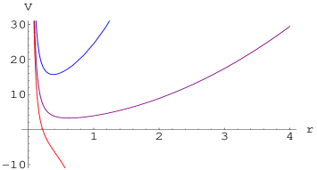
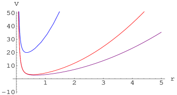
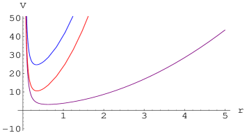
Figure 11: The potential vs horizon radius for $k=+1$. The values are fixed at $n=7$, $\lambda=17/4$, $\alpha=2/11$ (upper plot); $n=8$, $\lambda=14/4$, $\alpha=2/9$ (middle plot); $n=9$, $\lambda=9/4$, $\alpha=1/4$ (lower plot). The uppermost curve corresponds to the $\alpha=0$ case, and the two other curves correspond to $\mp$ signs in Eq. (79): $-$ and $+$ (upper and lower) in the uppermost plot, and the reverse in the lower two plots.

The hypergeometric equation (VI.1) may be solved exactly, and two independent solutions are

$$\Phi_{\pm}(x) = x^{(1\pm 2\nu)/4}\left(1+x\right)^{-\,i\omega/{2\sqrt{C}}}{}_{2}F_{1}\Bigg{(}\frac{\pm\,2\nu\mp 2\beta+2}{4}$$

$$-\,\frac{i\omega}{2\sqrt{C}},\frac{\pm\,2\nu\pm 2\beta+2}{4}-\frac{i\omega}{2\sqrt{C}};\pm\,\nu+1;-\,x\Bigg{)},$$

where $\nu=\frac{1}{2}\,\sqrt{4\lambda+(n-2)(n-10)}$ and $\beta=\frac{1}{2}\,\sqrt{n^{2}-8n+d}$. To determine the conditions for stability, with real $\nu$ and $\beta$, we need to satisfy

$$\lambda\geqslant\lambda_{crit}=\frac{1+(n-2)(10-n)}{4}\,,\quad d\geqslant 8n-n^{2}+1\,.$$ (83)

The first constraint is the same as in the $\alpha=0$ case, where $d=8n$, so $2\beta=n$. We may derive a more useful constraint for $C\alpha$ from the condition $d\geqslant(8n-n^{2}+1)$, so $2\beta\geqslant 1$, which implies that

$$C\alpha\leqslant\frac{(n-3)(n-1)}{2(n^{2}+11)}\,.$$ (84)

Using Eq. (79), along with $\Lambda=-\,n(n-1)/(2l^{2})$, we find

$$\frac{\alpha}{l^{2}}\leqslant\frac{(n-3)(n-1)(n^{2}+4n+19)}{4(n^{2}+11)^{2}}\,.$$ (85)

For $n+1=5$, one finds $\alpha/l^{2}\leqslant 17/324$. The bound $\alpha/l^{2}<17/324$ required here to keep the potential non-negative at the linearized level already puts a stronger bound to $\alpha/l^{2}$ than needed for thermodynamic (or dynamical) stability, namely, $\alpha/l^{2}\leqslant 1/12$.

By the same argument as for the pure AdS case with $\alpha=0$, the solution that is well behaved as $x\to\infty$ is given by the linear combination of $\Phi_{\pm}$, which reads

$$\Phi_{3}(x) = x^{-(2\beta+1)/4+i\omega/{2\sqrt{C}}}\,\left(1+x\right)^{-\,i\omega/{2\sqrt{C}}}$$ (86)

$${}_{2}F_{1}\Bigg{(}\frac{2\beta+2\nu+2}{4}-\frac{i\omega}{2\sqrt{C}},\,\frac{2\beta-2\nu+2}{4}$$

$$~{}~{}-\,\frac{i\omega}{2\sqrt{C}};\,\beta+1;\,-\,\frac{1}{x}\Bigg{)}\,.$$

In the $\alpha=0$ case, the leading behavior as $r\to\infty$ goes as ${\cal O}\left(r^{-(n+1)/2}\right)$, while as $r\to 0$ it goes as ${\cal O}\left(r^{1-2\nu)/2}\right)$. Both these solutions converge, and are normalizable only if $2\nu<1$, that is, if $4\lambda<1+(n-2)(10-n)$. However, in this limit, there may be a continuum of negative energy bound states due to a negative (or unbounded) potential. Fortunately, these solutions do not satisfy the usual boundedness condition

$$\int\phi^{2}\,\frac{r^{n-1}}{f(r)}\,dr=1,$$ (87)

because $\phi=\Phi\,r^{-(n-1)/2}\sim r^{-n}$ diverges at the origin. Thus, for the $k=+1$ case, a zero mass background is stable under tensor perturbations Gibbons02a , and this is true also for the $\alpha>0$ solution, in satisfying Eq. (85). In the latter case, the leading behavior of the solution as $x\to 0$ is given by ${\cal O}\left(x^{-(2\beta+1+2\nu-2\beta-2)/4}\right)\sim{\cal O}\left(r^{(1-2\nu)/2}\right)$. However, for the positive root in Eq. (79), the gravitational potential is unbounded when $n\leqslant 7$ and is unstable as in the $\Lambda=0$ case Deser85a .

VI.2 Potential for extremal background

For $\alpha>0$, the $\mu_{extr}<0$, $k=-1$ (extremal) background does not have constant curvature. The perturbation equations would involve terms like $a(l^{6}/r^{8})$ and higher powers of $(l/r)$, with some constant $a$, namely, $a\ll{1}$ when $\alpha\ll{l}^{2}$. This complicates the process for finding an exact solution to the Schrödinger equation. But, in the limit $\alpha\ll{l}^{2}$, as well as $r^{2}>2\alpha$, we may get some approximate ideas about the stability of an extremal background by inspecting the gravitational potential.

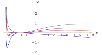
Figure 12: The potential vs horizon radius, with an extremal state as the ground state. The values are fixed at $n=4$, $l^{2}=1$, $\lambda=-1,\,-1.6,\,-2,\,-3$ (from top to bottom); and $\alpha=1/17$ (upper plot) and $\alpha=1/20$ (lower plot).

For $k=-1$, the gravitational potential, when $\alpha/l^{2}$ or/and $r^{2}>2\alpha$, may be given by

$$V(r) \simeq \Bigg{[}\frac{4\lambda+13}{4r^{2}}-\frac{17}{8\alpha}+\sqrt{\frac{(l^{2}-4\alpha)\,r^{4}}{(r^{4}-\alpha l^{2})\,l^{2}}}$$

$$\times \left(\frac{17}{8\alpha}-\frac{13\,l^{4}}{8(l^{2}-\alpha)r^{4}}\right)+\frac{4(2l^{2}-19\alpha)}{l^{2}(l^{2}-2\alpha)}\Bigg{]}f(r),$$

where one reads $f(r)$ from Eq. (78). For a small coupling $\alpha\ll{l}^{2}$, the gravitational potential (VI.2) can be bounded from below for all eigenvalues satisfying $\lambda>\lambda_{crit}=-\,13/4$. The coupling $\alpha/l^{2}$ is an equally important parameter for the dynamical stability of the background. As the plots in Fig. 12 show, when $\alpha/l^{2}\leqslant 1/18$ holds, the potential is bounded from below and is positive for large $r$, but it can be negative and unbounded for $\alpha/l^{2}>1/18$. It is quite interesting that the above constraint for $\alpha/l^{2}$, which we actually derived for $k=+1$, is also effective in the $k=-1$ case.

It is possible that the form of the gravitational potential would be modified at small scales, namely, $r^{2}<l^{2}/2$, due to terms like $l^{6}/r^{8}$, and also due to additional higher derivative curvature corrections, like $R^{4}$ terms. However, any corrections to the potential coming from them would contribute only in the order of $1/r^{8}$, so they will not destabilize the potential for large $r$, as well as for small $r$, but in the limit $\alpha\ll{l}^{2}$ and $r^{2}>2\alpha$.

For $k=-1$, the base manifold has negative curvature, so a negative potential does not imply instability of the background, if it can be bounded from below. We can be a little more precise here. The Breitenloher-Freedman bound $\lambda>-\,n^{2}/4$, which may be required for the positivity of energy (or unitarity) in AdS_n+1 spacetime, is $\lambda>-\,4$, when $n+1=5$. In our case, we must satisfy $\lambda>-\,13/4$, such that the potential is bounded from below and positive for large $r$, which gives a stronger bound for the stability of an extremal background than the Breitenloher-Freedman bound.

A bounded and positive potential implies that there are no unstable modes. For a small but non zero GB coupling, hyperbolic black holes whose ground state is the extremal metric with a negative mass may be stable under tensor perturbations. What we have shown here is that the extremal black holes are also local minima of the energy under small metric perturbations.

VII Discussion and Conclusion

In this paper, we have presented three important ideas together: (i) the choice of a ground state for AdS black hole spacetimes with flat, spherical, and hyperbolic horizons, (ii) the thermodynamic stability of hyperbolic AdS black holes, and (iii) the gravitational (or dynamical) stability of AdS black hole spacetime of dimension $D>4$ under linear (metric) perturbations.

Having clarified which backgrounds should be used for AdS black hole spacetimes with flat, spherical, or hyperbolic horizons, we computed the Gauss-Bonnet curvature corrections to the AdS black hole thermodynamics, using the standard regularization method of Refs. Hawking83a ; Witten98a , which follow by the subtraction of divergences from a reference state to which the black hole solution is asymptotically matched. The extremal black holes are found to be local minima of the energy for anti–de Sitter black hole spacetimes with hyperbolic event horizons.

AdS₅ hyperbolic black holes present some interesting features, such as that the free energy and the entropy are dependent on the Gauss-Bonnet coupling $\alpha$ but the total energy is not. This equally explores the possibility that the entropy and free energy of hyperbolic AdS black holes scale with the coupling of $\alpha^{\prime}$ corrections when going from strong to weak coupling limits, as in Emparan99b ; Klemm99a .

We have shown that, for thermodynamic stability of hyperbolic black holes, the specific heat and the extremal entropy have to be positive on the background. By considering free energy curves, the corresponding thermal phase diagrams are obtained for $n=4$ and $n=6$ in the limits of small and large Gauss-Bonnet couplings. Our results appear to suggest that the GB type corrections to the black hole thermodynamics do not give rise to a Hawking-Page transition as a function of temperature for flat and hyperbolic event horizons.

We have shown that a stable branch of small spherical black holes will occur when the coupling $\alpha$ is small. More specifically, in the AdS₅ case, a first order thermal phase transition may be observed for a small GB coupling, namely, $\alpha<0.0278\,l^{2}$. In addition, the Hawking-Page transition temperature decreases when the coupling of $\alpha^{\prime}$ corrections is increased. This behavior is seen in all spacetime dimensions $D\geqslant 5$.

We have also explored the gravitational (or dynamical) stability of higher dimensional AdS black hole spacetimes, with and without a Gauss-Bonnet term, against metric perturbations. Our result suggests that a base manifold ${\cal M}$ with a negative constant curvature can be unstable under tensor perturbations if the background is a massless topological black hole. For solutions of the Einstein-Gauss-Bonnet theory, one may have potentials which are positive and bounded from below, when the coupling constant $\alpha^{\prime}$ is small, that is, $\alpha\ll{l}^{2}$.

Appendix: Linearized Curvature Terms for $R^{2}$ Gravity

Under a linear perturbation

$$\bar{g}_{ab}\to g_{ab}=\bar{g}_{ab}+h_{ab}\,,\quad g^{ab}=\bar{g}^{ab}-h^{ab},$$ (A1)

with $|h^{a}\,_{b}|<<1$, the curvatures transform as IPN01d

$$R_{abc}\,^{d} \to R_{abc}\,^{d}-\bar{\nabla}_{[a}\bar{\nabla}_{|c|}h_{\,b]}\,^{d}+\bar{\nabla}_{[a}\bar{\nabla}^{d}h_{b]\,c},$$

$$+\,\frac{1}{2}\left(\bar{R}_{abe}\,^{d}h_{c}\,^{e}-\bar{R}_{abc}\,^{e}h_{e}\,^{d}\right),$$

$$R_{ab} \to R_{ab}+\frac{1}{2}\,\left(\Delta_{L}\right)h_{ab}-\frac{1}{2}\,\bar{\nabla}_{a}\bar{\nabla}_{b}h+\bar{\nabla}_{(a}\bar{\nabla}^{c}h_{b)\,c},$$

$$R \to R-\bar{R}_{ab}h^{ab}-\bar{\nabla}^{2}h+\bar{\nabla}_{a}\bar{\nabla}_{b}h^{ab},$$ (A2)

where $h=h_{p}^{p}$. The Lichnerowicz operator $\Delta_{L}$ acting on a symmetric second rank tensor $h_{ab}$ reads as

$$\left(\Delta_{L}h\right)_{ab}=-\bar{\nabla}^{c}\bar{\nabla}_{c}h_{ab}-2\bar{R}_{acbd}h^{cd}+2\bar{R}_{(a}\,^{c}\,h_{b)\,c}\,.$$ (A3)

Diffeomorphism under $h_{ab}\to h_{ab}+\bar{\nabla}_{a}\xi_{b}+\bar{\nabla}_{b}\xi_{a}$ implies a gauge invariance of the linearized theory. One of the physical gauges is the transverse (or harmonic) gauge

$$\bar{\nabla}^{a}\hat{h}_{ab}\equiv\bar{\nabla}^{a}\left(h_{ab}-\frac{1}{2}\,g_{ab}\,h_{c}^{c}\right)=0\,.$$ (A4)

The Lichnerowicz operator is then compatible with the transverse trace-free condition $h_{c}^{c}=\bar{\nabla}^{a}h_{ab}=0$. This gauge does not eliminate all of the gauge freedom, but does simplify the perturbation equations

$$\delta R_{ab}=\frac{1}{2}\,\left(\Delta_{L}\right)_{ab}.$$ (A5)

1. Background solutions

The Einstein field equations modified by a Gauss-Bonnet term and a cosmological constant $\Lambda$ are

$$R_{ab}-\frac{2\Lambda}{n-1}\,g_{ab}=16\pi G_{n+1}\,\alpha^{\prime}\left(\frac{1}{n-1}\,Hg_{ab}-2H_{ab}\right)\,$$ (A6)

where $H_{ab}=RR_{ab}-2R_{acbd}R^{cd}+R_{acde}R_{b}\,^{cde}-2R_{ac}R_{b}^{c}$ and $H=H_{a}^{a}$. For $\alpha^{\prime}>0$, the metric solution is

$$f(r)=k+\frac{r^{2}}{2\alpha}\left(1\mp\sqrt{1+\frac{8\alpha\Lambda}{n(n-1)}+\frac{4\alpha\mu}{r^{n}}}\right),$$ (A7)

where $\alpha=16\pi G\,(n-2)(n-3)\alpha^{\prime}$. For $k=+1$, the background (AdS vacuum) is given by the setting $\mu=0$. Then Eq. (A7) takes the form

$$f(r)=1+C\,r^{2}\,,\quad C\equiv\frac{1\mp\sqrt{1+8\alpha\Lambda/{n(n-1)}}}{2\alpha}\,,$$ (A8)

where $C$ has the dimension $(\mbox{length})^{2}$. This corresponds to a maximally symmetric space, namely,

$$R_{abcd}=-\,C\,\left(g_{ac}g_{bd}-g_{ad}g_{bd}\right).$$ (A9)

Then the cosmological constant is fixed as

$$\Lambda=-\,\frac{n(n-1)C}{2}\,\left(1-\alpha C\right).$$ (A10)

Finally, for a spherically symmetric solution, one has

$$f(r) = 1+\frac{r^{2}}{2\alpha}\left[1\mp\sqrt{1-4\alpha C(1-\alpha C)}\,\right]$$ (A11)

$$= 1+C\,r^{2}\,,\quad 1+\frac{r^{2}}{\alpha}-Cr^{2}\,.$$

By replacing $C$ with $1/{\ell}^{2}$, we find $f(r)=1+r^{2}/{\ell}^{2}$. Thus, for a spherically symmetric solution, the AdS vacuum of the Einstein theory is also the vacuum of the Einstein-Gauss-Bonnet theory, although the black hole solutions (which are given by $\mu\neq 0$) with $\alpha>0$ are very different from the solutions with $\alpha=0$.

2. Linearized equations

In the background of Eq. (A9), the variations of the curvature terms are given by

$$\delta\left(RR_{ab}\right) = -\,n(n+1)\,C\,\delta R_{ab}-nC\,\delta R,$$

$$\delta\left(R_{acde}R_{b}\,^{cde}\right) = -\,4C\,\delta R_{ab}+2C^{2}\left(h_{ab}-\bar{g}_{ab}\,h\right),$$

$$\delta\left(R_{a}^{c}\,R_{bc}\right) = -\,2nC\,\delta R_{ab}-n^{2}C^{2}\,h_{ab},$$

$$\delta\left(R_{acbd}R^{cd}\right) = \frac{nC^{2}}{2}\left((n+3)h_{ab}-\bar{g}_{ab}h\right)$$ (A12)

$$-\,(n-1)C\,\delta R_{ab}-\bar{g}_{ab}\,C\,\delta R,$$

and

$$\delta\Bigg{(}g_{ab}\Big{(}R^{2}-4R_{ab}R^{ab}+R_{abcd}R^{abcd}\Big{)}\Bigg{)}$$

$$~{}~{}~{}~{}~{}~{}~{}=\,n(n-2)(n-1)(n+1)C^{2}\,h_{ab}$$

$$~{}~{}~{}~{}~{}~{}~{}~{}~{}~{}~{}~{}-\,2(n-1)(n-2)\,C\,\delta R\,.$$ (A13)

Therefore, the field equations (A6) reduce to the form

$$\big{(}1-2C\alpha\big{)}\delta R_{ab} = -\,nC(1-C\alpha)\,h_{ab}+\frac{2(n^{2}+1)\alpha}{n-3}\,C^{2}\,h_{ab}$$ (A14)

$$-\,\frac{2\alpha\,C}{n-3}\,\Big{(}\delta R+C\,\bar{g}_{ab}\,h\Big{)}\,.$$

For an extremal metric background, however, Eq. (A14) may be used only for large $r$. For a small coupling $\alpha/\ell^{2}$, under the rescaling $l^{2}\to\ell^{2}/(1-\alpha/\ell^{2})$ in five dimensions, the extremal solution is

$$f(r)=-1+\frac{r^{2}}{2\alpha}-\frac{{\ell}^{2}-2\alpha}{2\alpha}\sqrt{\left(\frac{r^{4}}{{\ell}^{4}}-\frac{\alpha}{{\ell}^{2}-\alpha}\right)}\,.$$ (A15)

Therefore, in the limit $\alpha\to 0$, one has

$$f(r)\approx-1+\frac{r^{2}}{\ell^{2}}+\frac{\ell^{2}}{4r^{2}}=\frac{r^{2}}{\ell^{2}}\left(1-\frac{\ell^{2}}{2r^{2}}\right)^{2}.$$ (A16)

The solution with $\alpha>0$ is only asymptotically locally AdS; viz., when $\alpha={\ell}^{2}/5$, the curvatures are

$$R_{0}^{0} = -\,\frac{4}{{\ell}^{2}}-\frac{9}{64}\,\frac{{\ell}^{6}}{r^{8}}+{\cal O}\left(\frac{1}{r^{12}}\right)=R_{1}^{1},$$

$$R_{i}^{j} = \left[-\,\frac{4}{{\ell}^{2}}+\frac{3}{64}\,\frac{{\ell}^{6}}{r^{8}}+{\cal O}\left(\frac{1}{r^{12}}\right)\right]\delta_{i}^{j}\,.$$ (A17)

Although the subleading terms are much suppressed for $r>{\ell}$, for the extremal background there are extra contributions on the right hand side of Eq. (A14).

References

- (1) J. Maldacena, Adv. Theor. Math. Phys. 2, 231 (1998).
- (2) E. Witten, Adv. Theor. Math. Phys. 2, 253 (1998)
- (3) E. Witten, Adv. Theor. Math. Phys. 2, 505 (1998)
- (4) L. Vanzo, Phys. Rev. D 56, 6475 (1997).
- (5) D. Birmingham, Class. Quantum Grav. 16, 1197 (1999).
- (6) R. B. Mann, Class. Quantum Grav. 14, L109 (1997); gr-qc/9709039.
- (7) J. P. Lemos, Phys. Lett. B 353, 46 (1995); R.-G. Cai and Y. Z. Zhang, Phys. Rev. D 54, 4891 (1996); D. R. Brill, J. Louko, and P. Peldan, ibid. 56, 3600 (1997).
- (8) R. Emparan, J. High Energy Phys. 06, 036 (1999).
- (9) V. Balasubramanian and P. Kraus, Commun. Math. Phys. 208, 413 (1999).
- (10) R. Emparan, C. V. Johnson, and R. C. Myers, Phys. Rev. D 60, 104001 (1999).
- (11) G. T. Horowitz and R. C. Myers, Phys. Rev. D 59, 026005 (1999).
- (12) G. J. Galloway, S. Surya, and E. Woolgar, Phys. Rev. Lett. 88, 101102 (2002).
- (13) S. W. Hawking and D. N. Page, Commun. Math. Phys. 87, 577 (1983).
- (14) M. M. Caldarelli and D. Klemm, Nucl. Phys. B555, 157 (1999).
- (15) R. Emparan, Phys. Lett. B 432, 74 (1998).
- (16) A. Kihagias and J. G. Russo, J. High Energy Phys., 07, 027 (2000).
- (17) G. T. Horowitz and A. Strominger, Nucl. Phys. B360, 197 (1991); G. W. Gibbons and P. K. Townsend, Phys. Rev. Lett. 71, 3754 (1993).
- (18) G. W. Gibbons and S. A. Hartnoll, Phys. Rev. D 66, 064024 (2002).
- (19) R. C. Myers, Phys. Rev. D 36 (1987) 392.
- (20) D. G. Boulware and S. Deser, Phys. Rev. Lett. 55, 2656 (1985).
- (21) R. C. Myers and J. Z. Simon, Phys. Rev. D 38, 2434 (1988).
- (22) D. L. Wiltshire, Phys. Rev. D 38, 2445 (1988).
- (23) R.-G. Cai, Phys. Rev. D 65, 084014 (2002).
- (24) M. Cvetic, S. Nojiri, and S. D. Odintsov, Nucl. Phys. B628, 295 (2002).
- (25) Y. M. Cho and I. P. Neupane, Phys. Rev. D 66, 024044 (2002).
- (26) I. P. Neupane, Phys. Rev. D 67, 061501(R) (2003).
- (27) R.-G. Cai and K. Soh, Phys. Rev. D 59, 044013 (1999); J. Crisostomo, R. Troncoso, and J. Zanelli, ibid. 62, 084013 (2000); R. Aros, R. Troncoso, and J. Zanelli, ibid. 63, 084015 (2001).
- (28) A. H. Chamseddine, Phys. Lett. B 233, 291 (1989).
- (29) Y. M. Cho, I. P. Neupane, and P. S. Wesson, Nucl. Phys. B621, 388 (2002); Y. M. Cho and I. P. Neupane, Int. J. Mod. Phys. A 18, 2703 (2003).
- (30) H. S. Reall, Phys. Rev. D 64, 044005 (2001).
- (31) R. Gregory and R. Laflamme, Phys. Rev. Lett. 70, 2837 (1993).
- (32) S. Nojiri and S. D. Odintsov, Phys. Rev. D 66, 044012 (2002).
- (33) S. Surya, K. Schleich, and D. M. Witt, Phys. Rev. Lett. 86, 5231 (2001).
- (34) J. Polchinski, L. Susskind, and N. Toumbas, Phys. Rev. D 60, 084006 (1999).
- (35) A. Chamblin, R. Emparan, C. V. Johnson, and R. C. Myers, Phys. Rev. D 60, 064018 (1999).
- (36) I. P. Neupane, ICTP Report No. IC-2002-072; S. Nojiri and S. D. Odintsov, Phys. Lett. B 521, 87 (2001); 542, 301(E) (2002).
- (37) C. V. Vishveshwara, Phys. Rev. D 1, 2870 (1970).
- (38) V. Cardoso and J.P.S. Lemos, Phys. Rev. D 64, 084071 (2001).
- (39) G. E. Andrews, R. Askey, and R. Roy, Special Functions (Cambridge University Press, Cambridge, England, 1999).
- (40) R. Aros, C. Martinez, R. Troncoso, and J. Zanelli, Phys. Rev. D 67, 044014 (2003).
- (41) I. P. Neupane, Class. Quantum Grav. 19, 1167 (2002).